A vortex sheet based analytical model of the curled wake behind yawed wind turbines
Abstract
Motivated by the need for compact descriptions of the evolution of non-classical wakes behind yawed wind turbines, we develop an analytical model to predict the shape of curled wakes. Interest in such modelling arises due to the potential of wake steering as a strategy for mitigating power reduction and unsteady loading of downstream turbines in wind farms. We first estimate the distribution of the shed vorticity at the wake edge due to both yaw offset and rotating blades. By considering the wake edge as an ideally thin vortex sheet, we describe its evolution in time moving with the flow. Vortex sheet equations are solved using a power series expansion method, and an approximate solution for the wake shape is obtained. The vortex sheet time evolution is then mapped into a spatial evolution by using a convection velocity. Apart from the wake shape, the lateral deflection of the wake including ground effects is modelled. Our results show that there exists a universal solution for the shape of curled wakes if suitable dimensionless variables are employed. For the case of turbulent boundary layer inflow, the decay of vortex sheet circulation due to turbulent diffusion is included. Finally, we modify the Gaussian wake model by incorporating the predicted shape and deflection of the curled wake, so that we can calculate the wake profiles behind yawed turbines. Model predictions are validated against large-eddy simulations and laboratory experiments for turbines with various operating conditions.
keywords:
1 Introduction
Analytical models of various fluid mechanical phenomena in wind energy play an important role for basic understanding and for design and control of wind farms. Prime examples are models for the wind turbine wake velocity defect and its downstream evolution commonly used in wind farm layout optimization (Jensen, 1983; Stevens & Meneveau, 2017; Porté-Agel et al., 2020). In the classic Jensen model, for instance, a linearly expanding wake with a top-hat shape is assumed. More recent models allow for more realistic wake cross-sections with a Gaussian distribution (Bastankhah & Porté-Agel, 2014), and cross sections that transition from top-hat near the turbine to Gaussian further downstream have also been proposed (Shapiro et al., 2019).
Analytical wake models can be particularly useful in implementation of wake mitigation strategies such as wake steering, which has been receiving growing attention as an important control approach for increasing wind farm power output (Fleming et al., 2014; Gebraad et al., 2014; Bastankhah & Porté-Agel, 2015; Howland et al., 2016; Campagnolo et al., 2016; Schottler et al., 2017; Bartl et al., 2018; Lin & Porté-Agel, 2019; Kleusberg et al., 2020; Speakman et al., 2021). Achieving increased power output through wake steering involves turbines, often in the front rows of wind farms, being intentionally operated in yawed conditions to redirect their wakes away from downwind turbines. Although this reduces the power produced by the yawed turbines, research has shown that the total wind farm efficiency can improve as a result of more power generated by downwind turbines (Park & Law, 2016; Bastankhah & Porté-Agel, 2019; Fleming et al., 2019; Howland et al., 2019; King et al., 2021). Yawed turbine wake flows are known to exhibit complex features which makes their modelling more challenging than their unyawed counterparts. The most striking fluid-dynamic feature of a yawed turbine wake is arguably its curled cross-sectional shape (i.e., a kidney-shaped cross-section). This shape arises due to the action of a counter-rotating vortex pair (CVP) as detailed in Howland et al. (2016). CVPs are typically generated when forcing with strong spanwise gradients is applied perpendicular to the flow direction. One of the most notable examples are vortices trailing from finite-span wings that roll up and lead to the formation of a CVP, i.e. wingtip vortices or wake vortices in the aerodynamics literature. The formation and evolution of these vortical structures have been the subject of numerous studies since seminal works of Prandtl and Lancaster (See Anderson, 2011, and references therein). As noted in Bastankhah & Porté-Agel (2016), the CVP observed in yawed turbine wakes is also similar to those formed in many other free shear flows with strong spanwise variations of cross-wind velocity such as cross-flow jets (see e.g., the review of Mahesh (2013)).
In order to exploit the basic understanding of induced velocity and circulation of CVPs generated by finite-span wings, Shapiro et al. (2018) proposed to regard a yawed turbine as a lifting surface with an elliptical planform. Based on this approach, the lateral component of the thrust force can be regarded as the transverse lift force. This analogy made it possible to determine: (i) distribution of circulation at the yawed rotor modelled as a lifting line, and (ii) transverse velocity (equivalent to downwash velocity for finite-span wings) at the rotor disk due to the yaw offset. The latter enabled modeling of the transverse displacement of the wake but the wake itself was still assumed to retain a circular cross-sectional shape rather than the curled shape observed in practice. The associated vorticity distribution was later used by Martínez-Tossas et al. (2019, 2021) to develop a Lagrangian vorticity transport model that can predict the curled shape of the wake after numerical integration. Recently, Martinez-Tossas & Branlard (2020) and Zong & Porté-Agel (2020) have instead expressed rates of vorticity shedding at rotor blade tips using vortex cylinder theory (Coleman et al., 1945; Burton et al., 1995; Branlard & Gaunaa, 2016) to determine the trailing vorticity distribution behind a yawed rotor. The numerical model developed by Zong & Porté-Agel (2020) also takes into account the redistribution of point vortices in the wake due to their self-induced velocities. More recently, Shapiro et al. (2020) have solved the linearised mean streamwise vorticity transport equation to develop an analytical expression that can predict the decay of the CVP due to atmospheric turbulence. Bossuyt et al. (2021) have also experimentally demonstrated the impact of vortical structures shedding from a misaligned (either tilted or yawed) rotor on the curled shape of the wake downstream.
Capturing the curled shape of the wake for yawed turbines is of great importance since curling affects how much the wake will effectively overlap with downstream wind turbines, thus affecting the predicted power generation. However, models of the curled wake shape in the literature require numerical integration, and existing analytical wake models (e.g., Bastankhah & Porté-Agel, 2016; Shapiro et al., 2018; Qian & Ishihara, 2018; Blondel et al., 2020; King et al., 2021) cannot capture this deformation of the wake shape. There are several advantages to analytically expressed models that represent the trends in simple and explicit forms. Apart from their low computational cost, analytical flow models (Meneveau, 2019) often prove to be useful in revealing additional insights on flow physics that may not be evident using numerical simulation tools. Therefore, the current study aims at developing an analytical model to predict displacement and shape deformation of the wake behind a yawed turbine. The proposed model is inspired by prior works on two-dimensional vortex sheets (e.g., Rottman et al., 1987; Coelho & Hunt, 1989). The proposed analytical model predicts displacement and deformation of a vortex sheet, shedding from the circumference of a yawed rotor, as it is convected downstream. The vortex sheet model is then combined with a model for downstream evolution of wake velocity deficit to predict the shape of the curled wake and velocity distribution downwind of a yawed turbine.
The remainder of the paper is organised as follows. Section 2 derives the vortex sheet, truncated power-series solution for the yawed turbine wake in uniform, ideal flow, and model predictions are compared with numerical simulation under laminar uniform inflow. In §3, the model is extended to cases with turbulent boundary-layer inflow, and the results are compared with corresponding large eddy simulation (LES) data. Finally, §4 provides a summary of the developed model and our main conclusions.
2 Vortex sheet evolution in uniform, ideal flow
2.1 Evolving vortex sheet governing equations
As shown in Shapiro et al. (2020), among others, vortices shedding from the yawed rotor circumference represented as an actuator disk form a tubular vortex sheet. The objective of this section is to model the shape evolution of this vortex sheet with downstream distance or, equivalently, with time. Only the streamwise component of the shedding vorticity is modelled in this work because the lateral wake deflection and the deformation of the wake cross-section are mainly due to the velocities induced by the streamwise component of shedding vorticity (Martinez-Tossas & Branlard, 2020). The vortex sheet consists of semi-infinite streamwise vortex lines. In order to enable solving the governing equations analytically, following Coelho & Hunt (1989) and Rottman et al. (1987), we assume that the vortex sheet is planar and that its constituent vortex lines are infinite instead of semi-infinite, an approximation that improves at increasing distances from the origin.
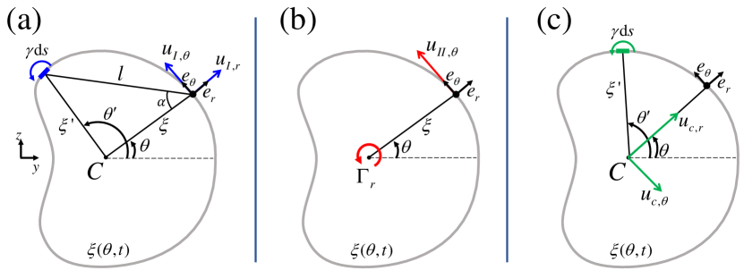
Figure 1 shows a schematic of the vortex sheet in the plane normal to the incoming flow. The coordinate system is defined with an origin at the rotor centre and with in the streamwise direction (i.e., parallel to the incoming flow) and and in the spanwise and vertical directions, respectively. Alongside this Cartesian system, we define a polar coordinate system of in the -plane (i.e., plane normal to the incoming flow). This polar coordinate system is attached to the centre of the vortex sheet, denoted by . The position of in the coordinate system is denoted by . As is the radial distance from , one can write . The polar angle is measured from the positive -axis toward the positive -axis such that . The shape of the vortex sheet is represented by the polar function that measures the distance of the vortex sheet from the centre, where is time. Our main objective is to describe the evolution of the vortex sheet as function of time in a frame moving downstream with the convection velocity , i.e. determine . This is equivalent to determining the downstream spatial evolution of the vortex sheet, with . The sheet location obeys
| (1) |
where , and denotes the radial velocity of the vortex sheet, which is affected by the strength of the evolving vortex sheet, whose evolution is treated next.
Let us denote the strength of the vortex sheet by , where the vortex strength is defined as the amount of circulation per unit length. In addition to the vortex sheet, there is a point vortex at with a circulation of (see figure 1b) to model the rotor root vortex, which is elaborated later in §2.3. We will show in §2.3 that the initial condition for the strength can be written as
| at | (2) | |||||
| at | (3) |
where and are constants depending on turbine operating conditions. Later in §2.3, we show that is related to the vorticity generated due to turbine yaw, while and are related to the vorticity generated by turbine rotating blades. Our focus now is to predict the deformation of the vortex sheet provided that the initial conditions are given by (2-3).
The velocity of the vortex sheet with respect to a coordinate system attached to the centre is given by
| (4) |
In (4) and hereafter, bold letters denote vectors. Next, we employ the Biot-Savart law to determine the three velocity terms on the right-hand side of (4), starting with the self-induced velocity , where and are unit vectors in the radial and tangential directions, respectively. The radial and tangential components of the self-induced velocity at a given polar angle of are respectively given by
| (5) | ||||
| (6) |
where and are defined in figure 1a, is a dummy integration variable, and . According to the law of cosines, The angle shown in the figure 1a can be related to based on the law of sines for the drawn triangle, which results in For small values of time and yaw angle , we can assume that the vortex sheet is approximately circular and thus . After some trigonometric manipulations, (5) and (6) can be simplified to
| (7) | ||||
| (8) |
Both integrals in (7) and (8) have singularities at and thus we use the Cauchy principal values (p.v.) of these two integrals. While the p.v. of the latter can be simply obtained by removing from the numerator and the denominator, the p.v. of the former needs to be determined for a given .
Next, we determine the velocity of the vortex sheet induced by the point vortex at C as shown in figure 1b. We obtain
| (9) | ||||
| (10) |
Finally, we determine , which is the velocity of induced by the vortex sheet, shown in figure 1c. It can be readily shown that is given by
| (11) | ||||
| (12) |
If we neglect streamwise (-direction) straining, vorticity is a conserved quantity, so the vorticity transport equation for the vortex sheet strength provides the additional required evolution equation (Moore, 1978):
| (13) |
where is the arclength along the vortex sheet. At small values of time and yaw angle , the vortex sheet remains approximately circular, so and can be respectively replaced with and . Therefore (13) is simplified to:
| (14) |
2.2 Analytical solution using power series approximation
We write , , and as power series in the form of
| (18) |
According to (1), for and the factor in (17), we have:
| (19) | ||||
| (20) |
where s are Taylor series expansion coefficients of . For example, the first three coefficients, which are used in the final solution of this paper, can be shown to be: , and . We insert the power series (18) and (20) into (15)-(17) and equating coefficients we obtain
| (21) | ||||
| (22) | ||||
| (23) |
The first term on the right-hand side of (21) is a Cauchy principal value (p.v.) of an improper integral. The following identities are useful to solve this integral:
| (24) | ||||
| (25) |
where , , and . The complete derivation of these integrals can be found in the appendix A.
From (2), . One can insert into (21) and (22) to respectively find and . Values of , and can be then inserted into (23) to find . This recursive process is repeated until reaching the desired order of evaluation for the power series of (18). After is obtained using the developed recursive relations, the dimensionless shape of the vortex sheet is evaluated from (19). The solutions for , and up to and for up to are written below
| (26) |
| (27) |
| (28) |
| (29) |
One can compute higher-order terms of (26)-(29), which may become relevant at increasing values of . However, since the above solution is developed based on the assumption that the vortex sheet remains approximately circular, increasing deformation of the vortex sheet makes the solution inaccurate at large values of . For practical applications at large , in Appendix B we propose an empirical formula that merges smoothly with the theoretical expression at small (i.e., 2), while it has desired reasonable properties at large times (i.e., 2). In the next section, we prove the validity of the initial conditions in (2) and (3). Moreover, values of , and are determined as functions of turbine operating conditions.
2.3 Setting vortex sheet initial conditions at yawed turbine location
In this section, we determine the vorticity shedding from a yawed rotor disk (i.e., ). According to Kutta-Jokowski theorem, lift force is proportional to the amount of circulation around a lifting airfoil. This means that an airfoil can be replaced with a bound vortex. Also, for any airfoil with finite span, free vortices must trail downstream from both sides of the bound vortex to infinity, forming a horseshoe vortex (Anderson, 2011). Turbine blades rotate and produce power due to their generated lift force, and vorticity is shed from the root and the tip of rotor blades. In addition, the whole yawed rotor can be assumed as a big finite-span airfoil with the lateral component of the thrust force regarded as the lift force. Therefore, in order to find the total shedding vorticity at the rotor disk, we need to determine those due to both yaw offset and rotating blades. In the following, we assume that the yawed rotor can be modelled as a rotating actuator disk.
2.3.1 Vorticity shedding due to turbine yaw
Prior studies have suggested two different approaches to model the distribution of circulation at a yawed disk. By modeling a yawed disk as a lifting line, the circulation is concentrated on a vertical line at the centre of the rotor with an elliptical distribution spanning from the bottom tip to the top tip of the rotor (Shapiro et al., 2018). Alternatively, vorticity due to yaw offset can be assumed to shed from the circumference of the rotor (Zong & Porté-Agel, 2020). Martinez-Tossas & Branlard (2020) used vortex cylinder theory to state the equivalency of these two methods. Shapiro et al. (2020) proved that both vorticity distributions yield the same induced velocity inside the radius of the rotor disk. To determine the reference circulation density needed in (2) and to provide more physical insight, we build upon the literature to show that the equivalency of these two vorticity distributions can be also verified simply by rearranging the position of horseshoe vortices over a yawed disk.
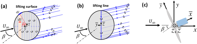
Figure 2a shows a schematic of a yawed actuator disk modelled as a lifting surface with a constant vortex strength of in -direction. The coordinate system is defined based on the rotor plane as shown in figure 2c, and its respective polar coordinate system () is defined such that and . The lifting surface shown in figure 2a can be envisaged as a surface with an infinite number of horseshoe vortices uniformly distributed across the yawed disk. The bound circulation at a given vertical position is given by
| (30) |
where is the rotor radius. Note that according to (30), the vertical distribution of the bound circulation for the lifting surface with a constant vortex strength is elliptical. This means that if we concentrate all these horseshoe vortices on a vertical line at the centre of the disk, the lifting surface is transformed to a lifting line with an elliptical distribution of circulation, like the one used by Shapiro et al. (2018), as shown in figure 2b. In this case, trailing vortices shed from all along the lifting line, because it consists of horseshoe vortices that vary in size. From (30), the maximum value of bound circulation for the lifting line, denoted by , occurs at at , and its value is equal to . From the lifting line theory, we know that (Shapiro et al., 2018), where is the turbine thrust coefficient. The value of is given by
| (31) |
where is the total magnitude of the turbine thrust force, is the air density and is the inflow velocity at the hub height. Note that this definition is the same as the one used in Shapiro et al. (2018), but it is different from the one used in some other prior studies (e.g., Burton et al., 1995; Bastankhah & Porté-Agel, 2016). Since , the value of is given by
| (32) |
Next, we determine the distribution of trailing vortices shedding from the circumference of the lifting surface. The circulation of the vortex shedding from an infinitesimal circumferential element , where , is . Given that , we obtain
| (33) |
For the lifting line, on the other hand, the magnitude of circulation of trailing vortex over the segment is equal to - (Anderson, 2011). From (30) and , we obtain
| (34) |
Using the variable change , one can easily show that for the lifting surface at any (33) is half of the one of the lifting line (34) at the respective height . Note that for the lifting surface, at a given height, trailing vortices shed at both angles of and with the same magnitude of circulation. Therefore, trailing vortices shedding from the lifting line and the lifting surface vary with height in a similar manner. It is also worth mentioning that the results presented here are in agreement with those obtained from the skewed vortex cylinder theory (Coleman et al., 1945; Branlard & Gaunaa, 2016). By modelling a yawed turbine wake as a skewed vortex cylinder, Martinez-Tossas & Branlard (2020) stated that the dominant vorticity shedding from the rotor is the tangential vorticity vector, which lies in the rotor plane. The streamwise projection of this tangential vorticity is equal to the one found in the present work (33) (c.f., equation 9 in Martinez-Tossas & Branlard (2020)).
2.3.2 Inclusion of wake angular momentum effects
In this section, we determine the value of required in (2) and (3). Based on the method of Joukowsky that models a turbine blade as one single horse-shoe vortex with constant bound circulation (see Okulov & Van Kuik (2012) for historical background), two free trailing vortices with the same magnitude of circulation are shed from both root and tip ends of each turbine blade. Under the assumption of large number of blades, this creates a vortex system consisting of a bound vortex disk, an axial root vortex and a tubular vortex sheet as shown in the figure 3a. Let us denote the circulation of the root trailing vortex with . As the amount of circulation along any horseshoe vortice remains constant, the bound circulation on the rotor disk at any radial position should be the same as . According to the Kutta–Joukowsky theorem, the bound circulation over an annular ring at a radial position and thickness of on the rotor disk generates a lift force , which amounts to (Okulov & Sørensen, 2010)
| (35) |
where is the resultant relative wind velocity experienced by the blade element as shown in figure 3b. In this figure, denotes the angle between and -direction, and is the component of in the -direction. The tangential component of produces power , which is given by
| (36) |
where is the turbine rotational velocity, and is the torque generated by the given annular ring. From the axial momentum theory, the power generated by the annular ring can be written as the product of and , where is the thrust force exerted on the annular ring. Therefore, we obtain an additional equation for as follows
| (37) |
Note that to derive (37), the local thrust coefficient for a given annular ring is assumed to be the same as its value for the whole rotor defined in (31). This is a correct assumption for the Joukowsky vortex model (Van Kuik et al., 2015). Equating (36) and (37) leads to
| (38) |
where is the tip-speed ratio and defined as .
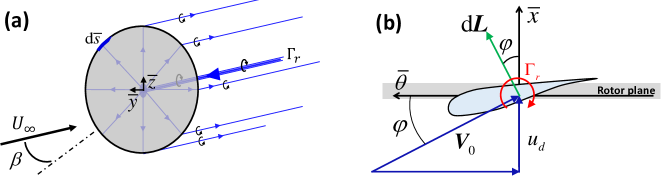
As seen in figure 3a, the trailing vorticity sheds over the circumference of the rotor disk. It is evident that the value of circulation for the vorticity shedding over the circumferential element is given by
| (39) |
where . The variable denotes the strength of the shedding tubular vortex sheet, and from (38),
| (40) |
It is important to note that as discussed by Branlard & Gaunaa (2016), the above-mentioned shedding vortices are actually in the direction of the wake centreline axis that forms an angle with the streamwise coordinate . Prior studies (e.g., Coleman et al., 1945) however showed that the angle between the wake centreline and the coordinate is expected to be much smaller than the turbine yaw angle. Therefore, we assume that both axial root and tip shedding vortices are in the -direction for simplicity.
2.3.3 Total vorticity shedding from a yawed turbine
From findings of §2.3.1 and §2.3.2, we can determine the total vorticity shedding from a yawed rotor due to both yaw offset and rotating blades as a function of turbine operating conditions. From (33) and (39), the value of the dimensionless initial vortex strength in the polar coordinate system is given by
| (41) |
| (42) |
The variable called the rotation rate is the ratio of the strength of vortex generation due to rotating blades to the one generated due to yaw offset. For the limiting cases of , is equal to zero, and the shedding vorticity is only due to the yaw offset. As the tip-speed ratio goes to infinity, the amount of torque generated by the turbine goes to zero. Therefore, according to the conservation of angular momentum, there should be no wake rotation downwind of the actuator disk in the limiting cases of . Hereafter, the term non-rotating wake refers to the wake of an actuator disk with an infinite tip-speed ratio , while rotating wake refers to the wake of an actuator disk with a finite value of .
2.3.4 Initial shape of the vortex sheet
The vortex sheet sheds from the circumference of the rotor, so it initially has a shape similar to the projected frontal area of the yawed disk, which is an ellipse with a semi-major axis of in the -direction, and a semi-minor axis of in the direction. The disk-averaged velocity normal to the rotor is equal to , where is the turbine induction factor, and it is given by (Burton et al., 1995). Behind the turbine, the rotor streamtube area expands further as pressure recovers to the background value (Manwell et al., 2010). At this location, the streamwise velocity is given by (Bastankhah & Porté-Agel, 2016; Shapiro et al., 2018). From continuity, , the ratio of the expanded streamtube area to the projected frontal area of the rotor is therefore given by
| (43) |
Neglecting the distance between the rotor and the end of the streamtube expansion, we set the initial wake area enclosed by the vortex sheet at to be the projected frontal area of the rotor times . Therefore, has an elliptical shape expressed by
| (44) |
For a small yaw angle , the vortex sheet initially has an approximately circular shape. Therefore, one can approximate with given by
| (45) |
2.4 Vortex sheet lateral deflection
The analytical solutions of the vortex sheet shape developed earlier are represented in the polar coordinate system, which is attached to the vortex sheet centre . Therefore, in order to fully determine the locus of the vortex sheet with respect to a stationary coordinate system, we also need to compute how and vary with time or downstream distance (i.e., wake deflection). From figure 1c, the Kutta-Joukowski theorem can be used to obtain
| (46) |
| (47) |
where and . Inserting from (26) into (46) and (47) and performing the integration lead to
| (48) |
| (49) |
From (49), the vertical displacement of is zero when (i.e., actuator disks with non-rotating wake) as expected from symmetry and consistent with prior experimental and numerical works (e.g., Howland et al., 2016; Bastankhah & Porté-Agel, 2016; Bartl et al., 2018). Comparison of (48) and (49) for nonzero values of shows that is nonzero but still considerably smaller than for small values of . Therefore, we neglect in this work for simplicity.
It is worth remembering that to derive the analytical solution for the deformation of the vortex sheet, we assumed that the shape of the vortex sheet does not largely deviate from a circle. Although this is an acceptable assumption for small values of yaw angle and time, it is less accurate for large values of times, when the vortex sheet rolls up and forms a CVP. As shown in figure 4a, based on (48), the value of may even decrease with an increase of , which is clearly unphysical. Since we expect that at large times (or downstream distances) a CVP can more realistically represent the vorticity shedding from the yawed rotor, we enhance our model for so that at large distances it tends to the situation of a CVP instead of using the truncated series vortex sheet solution.
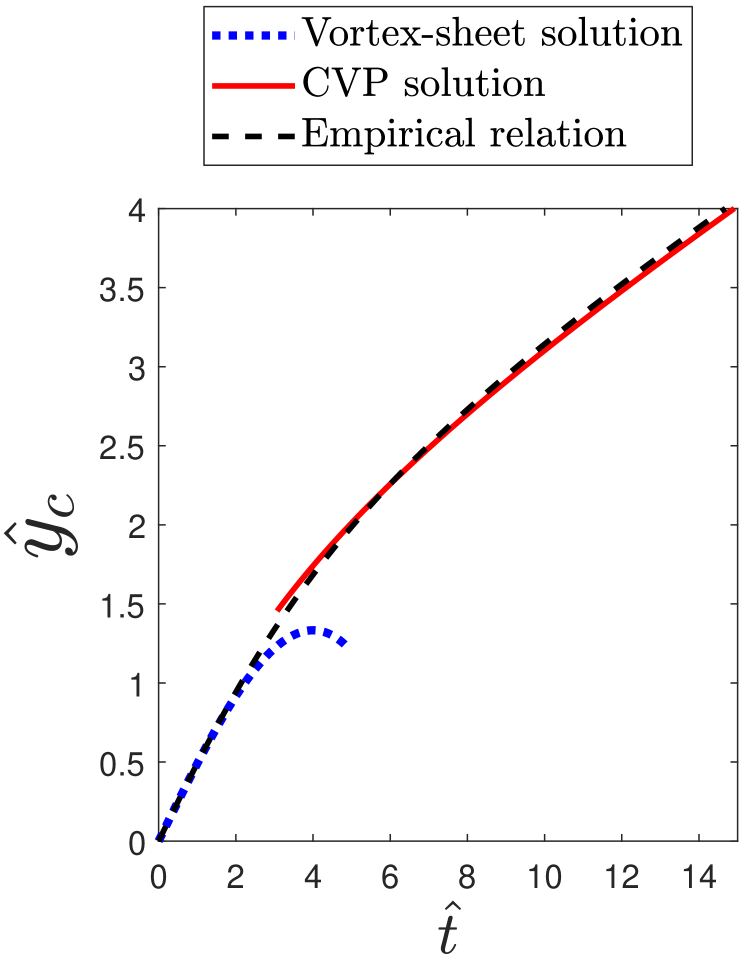
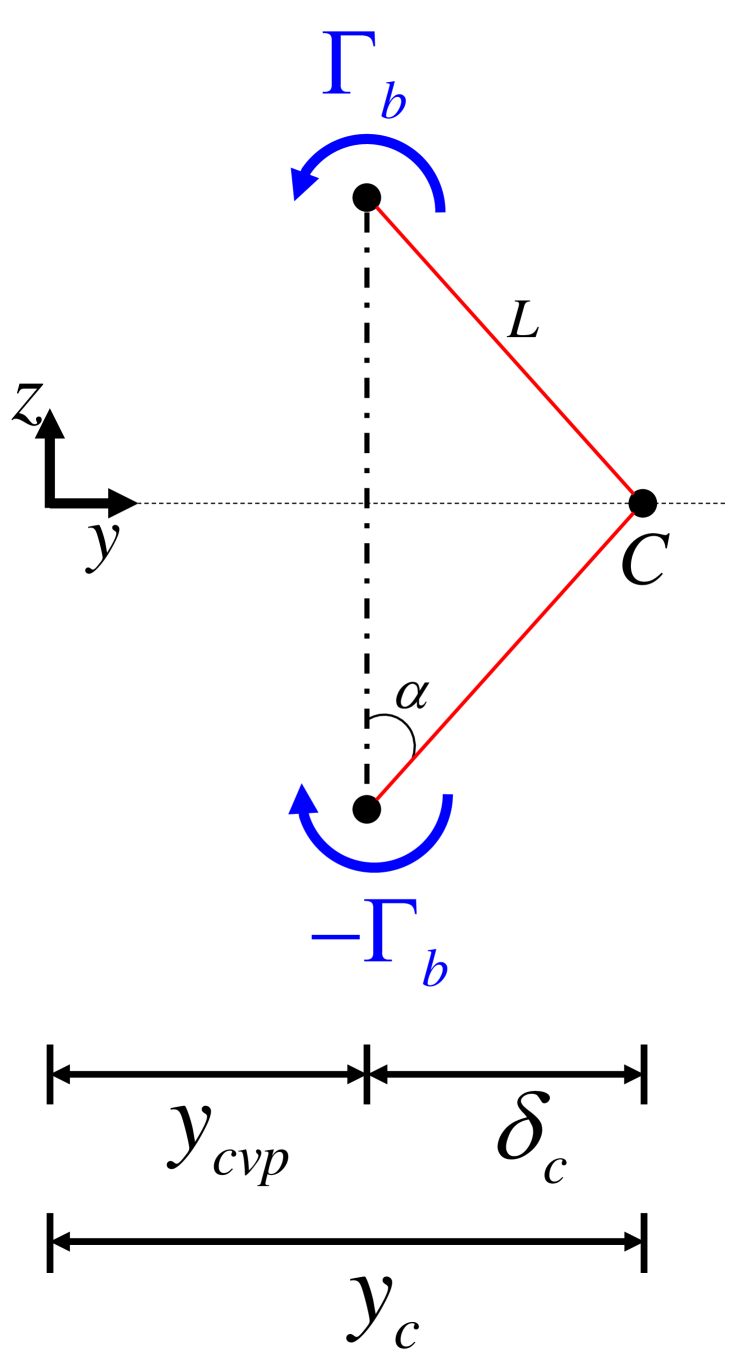
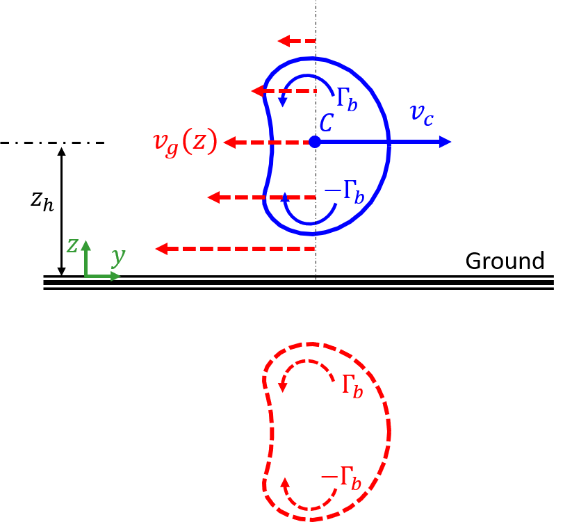
Figure 4b shows a schematic of a CVP. The CVP has the circulation of (Shapiro et al., 2018) as shown in figure 4b. The lateral position of the CVP is denoted by , and the lateral distance between the wake centre and the CVP is denoted by in the figure. The vertical spacing between counter-rotating vortices is equal to and it is assumed to remain constant. Initial values of , and are zero. In this analysis, only the vorticity shed due to the yaw offset is considered as the effect of shed vorticity due to rotating blades on the wake deflection is expected to be small. Our objective is to find the variation of with time (or downstream distance), but let us first determine how varies with time. According to the Biot-Savart law:
| (50) |
where is the lateral velocity of induced by the CVP, and and are defined in figure 4b. The CVP also moves with a lateral velocity of due to its self-induced velocity. Therefore, one can write
| (51) |
It is interesting to note that according to (51) increases until approaches . At this time and therefore the relative position of C with respect to the CVP does not change anymore, and remains equal to afterwards.
Next, we approximate in (51). We then integrate (51) (with separation of variables, and ) and write the solution in the dimensionless form. This yields an implicit expression for (it will be later expressed explicitly using an empirical formula):
| (52) |
where . Note that to derive (52), we assume . Given that , we have
| (53) |
Predictions of based on modelling the vortex sheet as a CVP using (52) and (53) are shown in figure 4a. As discussed earlier, the solution for based on the CVP is expected to provide acceptable predictions at large values of , while the solution based on an approximately circular vortex sheet (48) works better at short values of . An empirical formula that merges these two behaviors to leading order in both limits can be written as
| (54) |
where is the sign function of , and are polynomial coefficients, which need to be determined. Note that, similar to the vortex sheet and CVP solutions, the empirical relation is an odd function, so the wake deflection is opposite for turbines with opposite yaw angles. To find suitable values of polynomial coefficients (), we match the series expansion of (54) at and with and , respectively. This leads to a system of equations that needs to be solved. So we obtain
| (55) |
Equation (55) provides predictions similar to (48) at small values of and approaches (53) at large values of as shown in figure 4a.
2.5 Comparison with numerical simulations
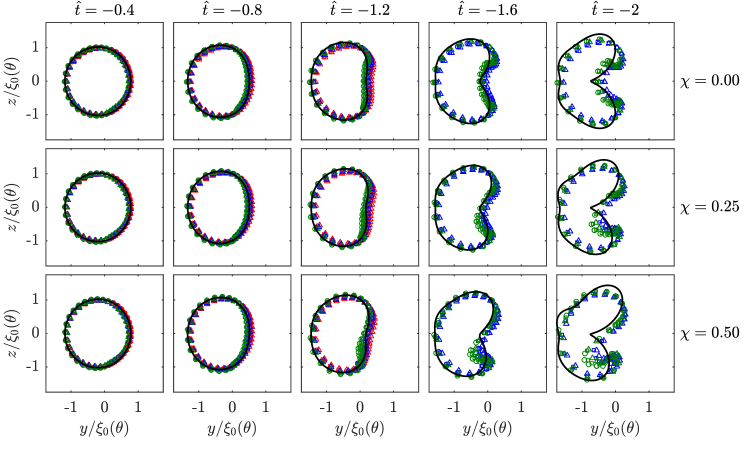
In this section, we compare predictions of the vortex sheet (i.e., wake edge) shape based on the new proposed model with numerical simulation data. For simulations, the pseudo-spectral large-eddy simulation (LES) code LESGO is applied. LESGO has been used in prior works (Calaf et al., 2010; Stevens et al., 2014; VerHulst & Meneveau, 2015; Stevens et al., 2018; Martínez-Tossas et al., 2018; Shapiro et al., 2018) to simulate flow past wind turbines and wind farms. It has been validated by detailed comparisons with several other LES codes (Martínez-Tossas et al., 2018). Turbines are simulated using the actuator disk model with rotation (ADM-R). See the Appendix C for more information about the LESGO code and the LES setup of this study. Under uniform inflow conditions the role of turbulence is minimal, and the code runs mostly as an inviscid solver with regularization, as it was also used in Shapiro et al. (2018). Simulations are performed for a range of local thrust coefficients and , yaw angles , , and , and rotation rates , 0.25, and 0.5. Note that according to (32) this means that and are negative and the curling is expected to be in the opposite direction of that shown in the sketch in figure 1, i.e. in the LES the wake is being deflected in the negative -direction. Also, it is worth remembering that the rotation rate depends on both yaw angle and tip speed ratio . According to (42), for a utility-scale wind turbine with a tip speed ratio and yaw angle , rotation rate varies between . The non-rotating case commonly used in the LES corresponds to an infinite tip speed ratio and reduces to the standards actuator disk model (ADM) without rotation. The local thrust coefficient is related to the thrust coefficient through (Shapiro et al., 2018). A fringe forcing region is used to force the flow back to laminar inflow when using periodic boundary conditions in the -direction. Excluding this fringe region the effective domain has sides that are , , and long. A uniform grid with effective grid points in the streamwise direction and grid points in the spanwise and vertical directions are used. The centre of the actuator disk is placed 3.6D from the inlet of the domain.
In order to determine the shape of the wake edge based on the developed model, we need to first compute the value of where can be approximated with (45) and . Although the convection velocity in turbine wakes changes with the streamwise distance, it is approximated with a constant value in this study, as done in prior studies (e.g., Shapiro et al., 2020). For cases with no incoming turbulence, the turbine wake does not significantly interact with the surrounding flow, and it experiences a slow recovery. In this case, the streamwise velocity profile in the central part of the wake can be modelled as a top-hat core (i.e., potential core) with a constant velocity equal to (Bastankhah & Porté-Agel, 2016; Shapiro et al., 2018), where is the incoming velocity. The top-hat core is surrounded by a shear layer in which the velocity changes from to . Therefore, we approximate the convection velocity with . For instance, based on this definition, (i.e., limiting value for using the analytical model) corresponds to a streamwise distance in the range of for a turbine with (i.e., for ), and .
The analysis presented in §2 suggests that the wake shape, non-dimensionalised by , only depends on the dimensionless time , and the rotation rate . As a first test of the model we compare the dimensionless model predictions with LES results normalized such that they can be presented as function of and . For the LES data, the edges of the wake are identified by tracking the edge of the streamtube that passes through the face of the actuator disk which is appropriate in this case due to the lack of turbulent mixing. Results are shown in figure 5, which shows that the LES data for turbines with different operating conditions approximately collapse onto the same wake profile curve for given values of and , in agreement with the proposed theory. The figure also shows that the proposed analytical model is able to capture the scaled wake shape. At larger time magnitudes and large rotation rates some discrepancies appear especially in the bottom right quadrant.The governing equations are developed by assuming small deviations of the vortex sheet from its initial shape. In addition, a severely truncated series expansion is used to solve governing equations. Therefore, the model cannot fully capture the vortex roll-up and transition of the vortex sheet to a counter-rotating vortex pair at large times, and some discrepancies are noticeable. For non-zero values of rotation rate, an additional level of vorticity sheds from the rotor circumference due to blade rotation. Given the sinusoidal nature of vorticity due to yaw offset (33), the additional shedding vorticity due to rotation increases the vorticity magnitude on either bottom or top halves of the wake (e.g., bottom half for the data shown in figure 5), which in turn accelerates the vortex roll-up. At larger values of rotation rate, discrepancy is thus expected to be higher due to the earlier occurrence of vortex roll up. This is confirmed in figure 5 by comparing model predictions at the same dimensionless time (e.g., ), but different values of rotation rate.
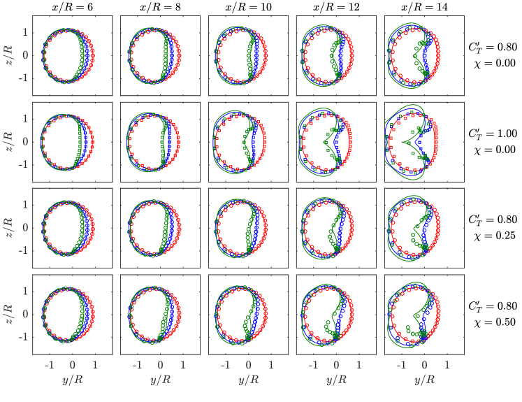
Next, we expand the comparison and plot the results in terms of physical parameters that are more directly related to the flow configuration: downstream distance , local thrust coefficient , yaw angle , and dimensionless rotation rate . Figure 6 shows wake edge predictions of the analytical model together with the LES data for different values of , and , at several downwind locations. The figure shows that the degree of wake curling increases with yaw angle, thrust coefficient and streamwise distance, as expected from the analysis presented in §2. Moreover, wake rotation breaks the vertical symmetry of the wake. The results presented in figure 6 show that the wake shape depends strongly on all of the varied parameters: thrust coefficient, yaw angle, and rotation rate. The analytical model developed is seen to agree well with the LES results, up to intermediate levels of wake curling. The analytical model successfully predicts the shape of the wake for various operating conditions. As the wake deformation grows further downstream or at increasing , differences appear, as mentioned before due to the limitations of the model that is based on a severely truncated series expansion. It is clear that there is reduced agreement in the lower half of the wake for cases with large values of yaw angle and rotation rate. As discussed earlier, for these cases the lower half of the wake cross-section is subject to a strong vortex roll-up caused by the cumulative vorticity due to both yaw offset and rotation. Still, the model is able to predict many qualitative features of the wake shape, including its vertical asymmetry for cases with rotation. In addition, the sideways displacement of the entire wake is also captured quite well in all cases.
3 Vortex sheet evolution in turbulent atmopsheric boundary layer
In this section we generalize the prior analytical model of a yawed wind turbine wake that is applicable for ideal non-turbulent flow to the case of a wake with a turbulent atmospheric boundary layer background flow. Here we seek a model for the entire mean velocity distribution as a function of downstream distance as well as cross-stream position, accounting for the fact that the wake will be curling due to turbine yaw.
3.1 Vortex sheet evolution in turbulent atmospheric boundary layer
For the ideal flow case, we assumed that the vortex sheet does not decay as it moves downstream, and the strength of the streamwise vorticity only evolves along the vortex sheet in time following idealised vortex dynamics. Although this may be an acceptable assumption for turbines with uniform non-turbulent inflows, it is not expected to be valid for turbines immersed in turbulent environments such as the atmospheric boundary layer (ABL). The vertically-varying mean inflow velocity in the ABL can be approximated as , where is the friction velocity, is the von-Kàrmàn constant, and is the roughness height. As discussed in Shapiro et al. (2020), the vorticity shedding from a yawed rotor decays due to the turbulent diffusion; i.e., and are functions of time. Instead of solving the full governing equations for diffusing vortex sheet, we approximate the effects of diffusion by scaling and the velocities by the circulation that is decaying according to a previously obtained analytical solution for the decay of CVP in a turbulent boundary layer (Shapiro et al., 2020). Specifically, we define new scaled variables , and such that
| (56) |
If one defines scaled displacement and time according to
| (57) | ||||
| (58) |
one recovers the original governing equations (15), (16) and (55) for the new definition of variables and . An additional term is however introduced in (17) , so
| (59) |
It will be shown later in (63) that , where , is a constant and is the expansion rate of the turbulent diffusive scale, and it is modelled as (Shapiro et al., 2020). So the Taylor expansion of is given by
| (60) |
For atmospheric flows, the value of at the hub height is equal to (Shapiro et al., 2020). Therefore, is a slow varying reference quantity, and the additional term on the right-hand side of (59) is neglected for simplicity. This means that the solution already developed in §2.2 will still be used as a model for the decaying vortex sheet once rescaled by the prescribed evolution and using the modified time . Note that for a constant , (56)-(58) become the same as dimensionless variables defined earlier for a non-decaying vortex sheet.
Next, in order to evaluate the integral of (58) and derive a relationship for under turbulent inflow conditions we need to specify a convection velocity under turbulent inflow conditions. Due to atmospheric turbulence, the wake mixes and recovers more quickly than in the laminar inflow case, and thus the mean velocity at the wake edge is comparable to the incoming velocity. We therefore assume that in this case the vortex sheet at a height is convected downstream with the incoming velocity at that height ; thus and .
To evaluate (58), we must specify the decay of vorticity, i.e. of with streamwise distance. In Shapiro et al. (2020) the decay of the total vortex circulation was studied, its relationship with the density being . The resulting derived model for the total vortex circulation as function of downstream distance is given by
| (61) |
where , is the modified Bessel function of the first kind with order , and is the turbulent diffusive scale, and is the virtual origin assumed to be zero in the current work for simplicity.
One can use , , and to rewrite (58) as
| (62) |
Numerical integration of , expressed by (61), yields results that can be conveniently approximated by the following (fitted) expression:
| (63) |
We then use (32) to express as a function of operating conditions, approximate with given by (45), and insert (63) into (62) to obtain
| (64) |
Due to vorticity decay, for turbulent inflow cases increases at a slower rate than the one for laminar inflow cases. For instance, according to (64), for a turbine with subject to an ABL with , the streamwise position associated with varies between and for . As mentioned in §2.5, for the same turbine with subject to a laminar flow, at . It is also worth noting that the above definition of (64) is reduced to the one used for non-decaying vortex sheets (i.e., ) as tends to zero.
The effect of the ground on the wake deflection was not modelled in the uniform inflow cases. To model the effect of the ground, we use an image technique to modify the wake centre location , as shown in figure 7. Modelling the vortex sheet as a CVP, the image CVP induces a lateral velocity in the opposite direction, termed as given by
| (65) |
Therefore, the lateral wake deflection caused by the ground is given by
| (66) |
Approximating and using we find
| (67) |
where . Substituting with in (67) for simplicity and subtracting this result from (55) yields
| (68) |
It is worth mentioning that for , the second term on the right-hand side of (68) vanishes, and thus the equation is reduced to (55).
3.2 Analytical model for mean velocity distribution
The shape of the wake edge predicted earlier can now be used to model the spatial distribution of the velocity deficit in the curled wake at each streamwise position. For non-curled (i.e., non-yawed) wakes a number of wake profiles have already been proposed in the literature, including top-hat (Katić et al., 1986; Frandsen et al., 2006), Gaussian (Bastankhah & Porté-Agel, 2014, 2016), double Gaussian (Schreiber et al., 2020), and super-Gaussian (Shapiro et al., 2019; Blondel & Cathelain, 2020). Most of these conserve flux of momentum deficit only in its linearized version valid far downstream, see discussion in Bastankhah & Porté-Agel (2014). Here we demonstrate the use of the shape deformation for an analytical model in the context of the Gaussian wake model (Bastankhah & Porté-Agel, 2014, 2016), but it could be implemented in other wake models as well.
The modeled streamwise mean velocity
| (69) |
is defined based on the incoming velocity field and the modeled velocity deficit in the wake, . In the Gaussian model, the velocity deficit profile is modeled as
| (70) |
where is the normalised maximum velocity deficit at each streamwise location and is the characteristic wake width. In (70), the wake centre location is , where is obtained from (68) and is approximated with given in (45). In prior versions of the Gaussian wake model, it is assumed that the characteristic wake width depends only on downstream distance. Moreover, it is assumed that it grows linearly downstream at a rate . The linear growth of the wake arises from the similarity solution when eddy-viscosity is assumed to scale with a constant velocity, friction velocity , and the wake scale itself (Shapiro et al., 2019), i.e.
| (71) |
where is the wake expansion rate and the initial wake size. We now propose to include wake curling and deformation by making dependent also on the angle according to
| (72) |
where , and is given by (44), and the dimensionless wake shape is given by either the analytical relation of (29) for or the empirical relation (89) for given values of polar angle and dimensionless time . The polar angle is determined at each position from , and is given by (64). In (72), the first term on the right-hand side of the equation expands the wake in all radial directions due to turbulent mixing, while the second one deforms the wake cross-section according to the vortex sheet solution derived earlier. According to (72), for an unyawed turbine, the initial characteristic wake width is reduced to , which is the same as the one suggested by Bastankhah & Porté-Agel (2014). For the wake expansion rate, we assume (Shapiro et al., 2019), where is an empirical constant. Alternatively, can be estimated based on the turbulence intensity of the incoming boundary layer flow (i.e., , where is an empirical constant) as suggested in prior studies (see Niayifar & Porté-Agel, 2016; Carbajo Fuertes et al., 2018; Zhan et al., 2020, among others). At each height , turbulence intensity is defined as , where is turbulent fluctuation of streamwise velocity, and overbar denotes time averaging. Note that invoking the logarithmic law for the fluctuating velocity variance in high Reynolds number turbulent boundary layers (Marusic et al., 2013; Meneveau & Marusic, 2013), one can show that and are related to each other by , where is the boundary-layer thickness, and and are constants.
The maximum velocity deficit in (70) is obtained by enforcing the conservation of streamwise momentum deficit flux . To simplify the integration and avoid dependence on , we approximate with where the latter is given by
| (73) |
In this expression, is given by (45) and is the wake expansion rate at . This yields
| (74) |
Note that in stating conservation of flux of streamwise momentum deficit, pressure and turbulent and viscous shear stress effects are assumed to be negligible. This may be a questionable assumption in the near wake region as well as far wake of turbines deep inside a wind farm (Bastankhah et al., 2020).
For the sake of completeness, a summary of the steps required to implement the proposed model and predict wake velocity deficit distributions at a given downwind location is provided below: (1) Compute the approximate form of the initial wake shape (45). (2) Determine the dimensionless time from (64). (3) Find the wake centre location , where is given by (68). (4) Find the polar angle , which is measured from the positive -axis toward the positive -axis such that . (5) Evaluate the initial wake shape (44). (6) Calculate the wake shape function , where can be estimated either from the analytical solution (29) (if ) or the empirical one (89), and is given by (42). (7) Find the wake width based on (72). (8) Evaluate the maximum velocity deficit from (74), where is given by (73). (9) Determine the wake velocity deficit according to (70).
3.3 Comparison with large eddy simulations
In the following, the streamwise mean velocity distribution based on the proposed model is compared with the LES data for turbulent ABL inflow cases. Simulations of yawed wind turbines represented as rotating actuator disks (ADM-R) are performed using and a local tip speed ratio of at yaw angles of , , , and (Shapiro et al., 2020), where the local tip speed ratio is defined as . In unyawed conditions, the selection of local thrust coefficient and tip speed ratio corresponds to and , which are realistic of modern utility-scale turbines. The actuator disk with diameter m and a hub height of m is placed 500 m from the inlet of a domain with an effective size of km, km, and km. The domain is divided into , , and grid points. The velocity field is averaged for a time , where m/s. A shift is used to reduce streamwise streaks in the time-averaged velocity field. The roughness height is m.
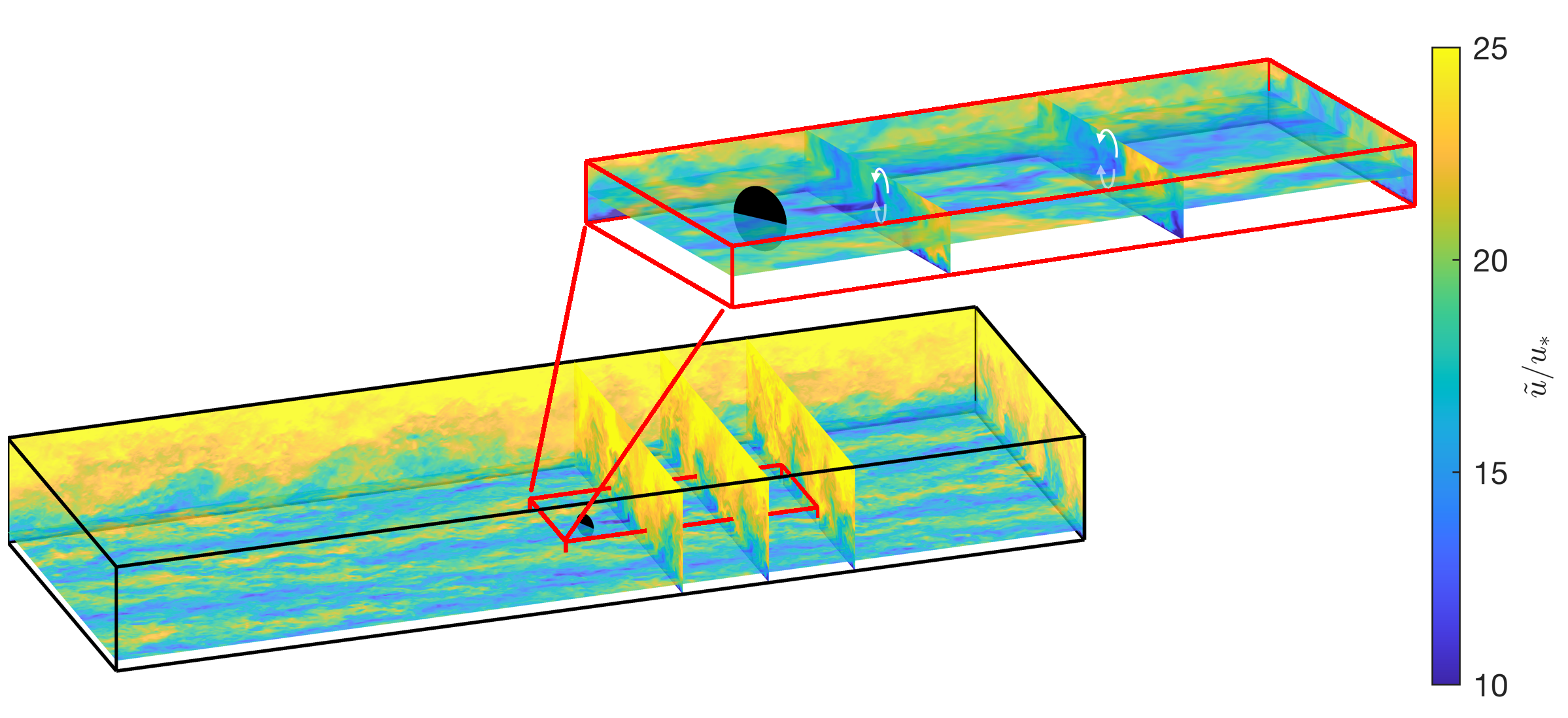
Figures 8 show contour maps of streamwise velocity on representative planes across the LES domain. It shows the streaks in the turbulent atmospheric boundary layer at the turbine hub height and the generated wake behind the yawed wind turbine, which is shown as a black circle. At downstream locations, the effect of the the curled yawed wind turbine wake on the cross-plane velocity field is shown at downstream locations of , , and .
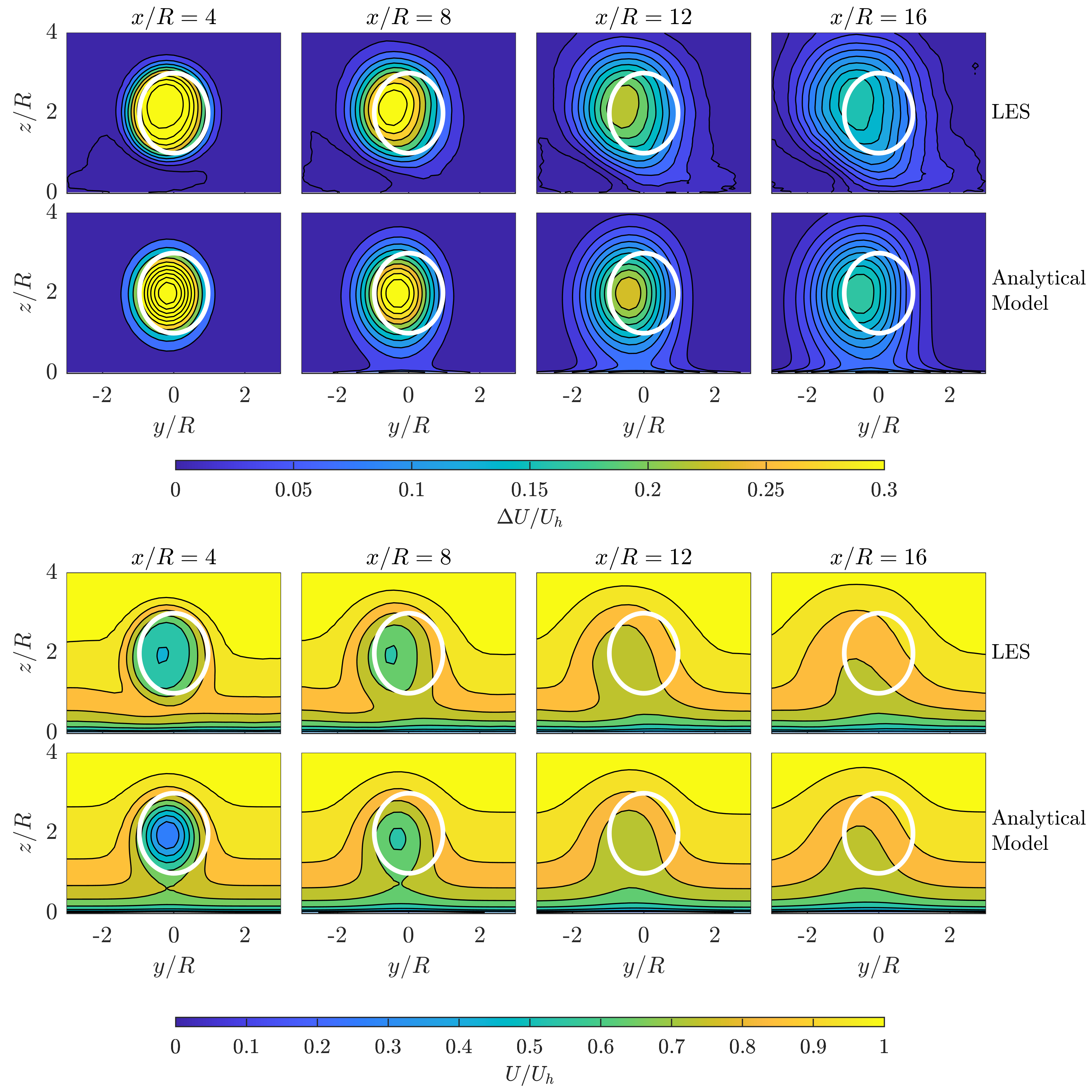
Figures 9 and 10 show the wake mean velocity distributions based on the LES results and the analytical model for and at various downstream locations. Top panels show the normalised velocity deficit and bottom panels show the normalised streamwise velocity distribution.
As in past studies (Bastankhah & Porté-Agel, 2016; Shapiro et al., 2018), the wake recovery rate in the analytical model is calculated by fitting a Gaussian profile to the downstream wake profiles at . This gives the resulting wake expansion rate as . As seen in figures 9 and 10, the model captures the curling and deflection of the wake as well as some variation in the wake deflection as a function of vertical distance due to ground effects. The LES results display slightly less curling than the model as well as more noticeable wake deflection towards the ground that is opposite to the deflection of the bulk of the wake. The analytical model does not also predict small vertical wake deflections observed in the LES data. According to the vortex sheet analysis performed in the current study (see (49)), this vertical deflection is due to rotation effects (i.e., non-zero values of rotation rate ). As mentioned in §2.4, for simplicity we did not include the vertical wake deflection in the final version of the model. Despite these small differences, figures 9 and 10 show that overall model predictions are in acceptable agreement with the LES data.
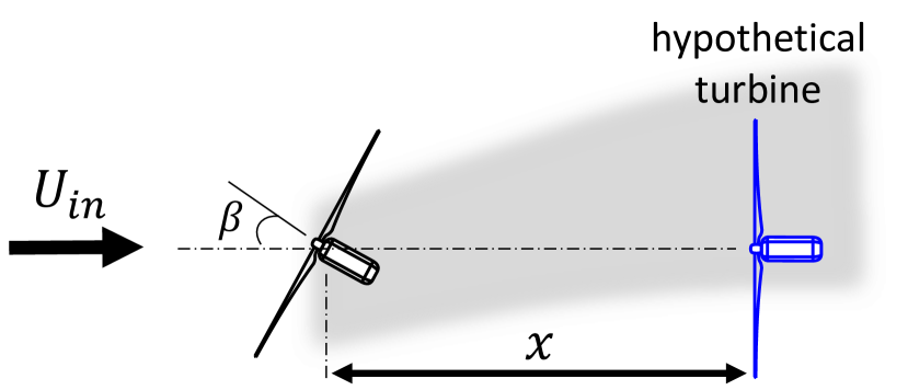
Wake flow results are also used to compute the power of a downwind turbine based on both the proposed analytical model and the LES data. In both cases, a virtual wind turbine is placed in the flow field at different distances downstream of the yawed turbine. The idea is that as yawing increases, the downstream turbine will overlap less and less with the wake due both to the sideways displacement of the wake and to the curled crescent shaped wake that creates lower velocity deficit at the centre of the hypothetical downstream turbine.
In order to evaluate the power generated by the downwind turbine, we require the disk-averaged streamwise velocity defined according to
| (75) |
where is the mean velocity in the flow at the turbine location computed from the model or from the LES and the integration covers the turbine disk area. For the latter case, we evaluate the mean velocity by time averaging: . Since the turbine is not included in the simulation, the turbine disk velocity that would occur there includes the prefactor, where is the turbine’s assumed induction factor. The power is subsequently calculated as
| (76) |
and it is normalized by the power that an unyawed free-standing turbine would generate under similar conditions, (thus making the result independent of assumed , etc.).
Figure 11 shows the normalised power of this hypothetical turbine as a function of streamwise spacing for different yaw angles of the upwind turbine. The figure demonstrates good agreement between the analytical model and the LES results for a broad range of streamwise spacings and yaw angles.
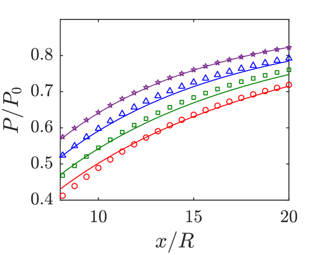
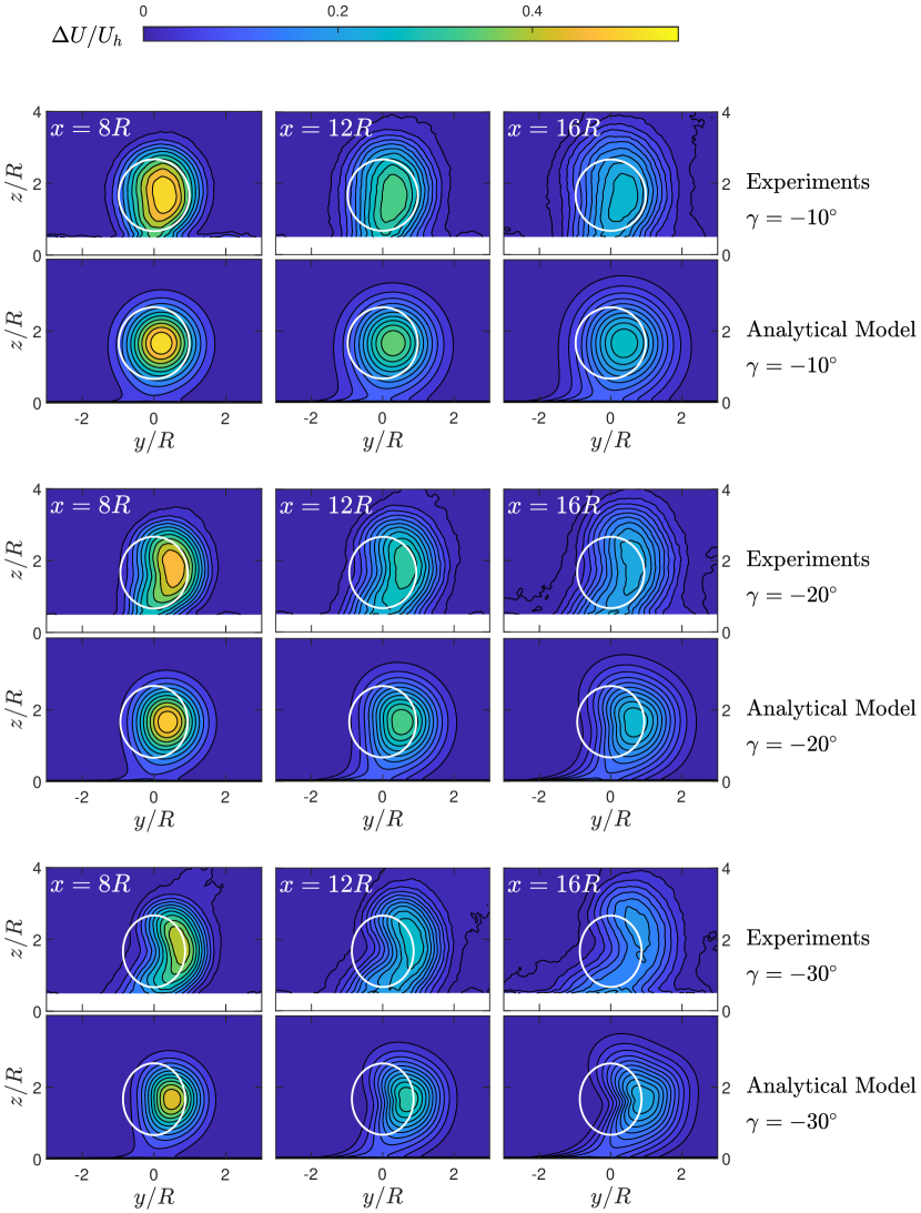
3.4 Comparison with experimental data
Model predictions are also compared with wind-tunnel experiments by Bastankhah & Porté-Agel (2016). Flow measurements were performed to quantify the wake of a yawed wind turbine with a diameter of cm and hub height of cm, and the turbine is subject to a turbulent boundary layer, naturally developed over the smooth surface of the wind-tunnel floor. Additional information on turbine properties (, , etc.) and inflow conditions (, , etc.) may be found in Bastankhah & Porté-Agel (2016). The wake recovery rate for the analytical model is estimated based on (Carbajo Fuertes et al., 2018). Figure 12 shows contours of normalised velocity deficit in planes at different downwind locations and different yaw angles based on both experiments and model predictions. Overall the figure shows that the proposed model is able to successfully predict the complex curled shape of the wake and its lateral deflection. The opposite wake deflection close to the ground is also well captured by the model. While the overall trends and qualitative features of the velocity defect distribution of the curled wake are reproduced by the analytical model, some differences between measurements and model can still be discerned. The figure shows that the vertical extent of the lower half of the wake is underestimated by the analytical model, which is mainly due to neglecting the wake of the turbine tower in the analytical model. Tower wake effects are however expected to be less significant for utility-scale wind turbines which tend to have less bulky towers (with respect to the rotor diameter).
4 Summary and conclusions
A curled shape is a typical aerodynamic feature of wakes behind yawed turbines. In this study, we develop an analytical model to describe the wake shape and its downstream evolution for both uniform ideal inflow and turbulent boundary layer background flow. The predicted wake shape is then used in a wake model to describe analytically the mean velocity deficit distribution behind a yawed wind turbine.
To model the curled shape of the wake, we represent the wake edge as a vortex sheet shedding from the rotor disk circumference due to both yaw offset and rotation. A simple relationship is developed to estimate the initial distribution of vorticity along this vortex sheet as a function of turbine operating conditions such as thrust coefficient, yaw angle and tip-speed ratio. The goal is to obtain the evolution of the locus of this vortex sheet with time. The governing equations for the deformation of the vortex sheet are developed based on the Biot-Savart law and the vorticity transport equation. After non-dimensionalising the equations, they are solved using a power series expansion method. Subsequently, assuming a given downstream convection velocity, we map the time evolution to a spatial one in the streamwise direction. The developed solution is only valid for limited range of dimensionless times () or equivalent distances. For larger values of , an empirical expression is also proposed, which complies with the derived analytical solution for smaller times but is also realistic for larger times.
Apart from deforming to a curled shape, the vortex sheet is also deflected laterally behind a yawed turbine. This deflection is modelled with an equation combining analytically derived deflections using two approaches: considering an approximately circular vortex sheet (valid for small times) and considering self-induced motion of a CVP (valid for larger times). Moreover, close to the ground the wake is deflected in the opposite direction. This ground effect is modelled using image flow that introduces an additional deflection term to account for the velocity induced by the image CVP.
Wake shape predictions are first compared with numerical simulation data for a yawed turbine placed in a uniform, non-turbulent inflow. Several cases with different values of thrust coefficients, yaw angles and tip-speed ratios are considered. It is shown that the analytical model predictions agree well with LES results at moderate times. Also in agreement with the theory, we show that the numerical simulation results can be collapsed into a common wake shape when the problem variables are normalised using the scaling as suggested by the theoretical model.
The theory is then adapted to the case of turbulent ABL inflow for applications to real wind turbine flows. It is known that, unlike the case of ideal flow, turbulent diffusion plays a central role in weakening the streamwise vortices during their downstream evolution. This phenomenon is modeled by non-dimensionalizing the governing equations using a time-varying reference vortex sheet strength. Finally, we modify the Gaussian wake model to incorporate the predicted shape and lateral deflection of the curled wake. The analytical curled wake model thus describes the full spatial distribution of mean streamwise velocity downstream of a yawed turbine. To validate the model predictions for the ABL case, wake velocity contours at different downstream positions are compared with LES and wind-tunnel results at various yaw angles. Moreover, the power extracted by a hypothetical wind turbine located at different downwind positions is computed and compared to similar results from the LES-generated mean velocity distributions. A good agreement of the model predictions with the numerical and experimental data is observed, suggesting that the proposed model includes the most relevant fluid mechanical effects governing the mean velocity distribution in wakes downstream of yawed wind turbines. Also, the proposed analytical model should be useful for tasks such as wind farm optimization and control, where numerical simulations tend to be too time consuming and costly. While to our knowledge the developed analytical model is the first of its kind to predict the curled shape of yawed turbine wakes, more research is still needed to shed light on the impact of ABL characteristics such as wind veer on the wake of a yawed turbine. Of special interest is to study the combined effect of yaw offset and wind veer on the wake cross-section in future works. Moreover, the effect of ground and rotation on the wake cross-section needs to be thoroughly studied in future works for turbines with different geometries and operating conditions.
Acknowledgements
MB acknowledges funding from Innovate UK (grant no. 89640). CS, DG and CM acknowledge funding from the National Science Foundation (grant nos. 1949778) and computational resources from MARCC and Cheyenne (doi:10.5065/D6RX99HX).
Declaration of interests
The authors report no conflict of interest.
Appendix A Evaluation of principal value of required integrals
This appendix evaluates the integrals (24) and (25). Here, we only provide the proof for (24), as (25) can be solved similarly. First, we define as
| (77) |
By defining the complex parameters and and the complex variable , and considering that , and , the integral can be written as:
| (78) |
where is the integration path, which is the unit circle, , on the complex plane, and is defined as:
| (79) |
In order to evaluate the integral in (78), we need to calculate the residues of at its singularities. has two singularities: one at (pole of order ) and the other at (pole of order one). To calculate the residue of at , we define a function such that (see Ablowitz & Fokas, 2003, chapter 4):
| (80) |
Therefore the residue at is:
| (81) |
or
| (82) |
It can readily be shown that the first derivative term is non-zero only for and . Also expanding the second derivative, and after some manipulation, we obtain:
| (83) |
Now we calculate the residue of at . To do this, we define a function such that:
| (84) |
Therefore the residue at is:
| (85) |
Since the second singularity is located on the integration path, we cannot use Cauchy Residue Theorem directly. However, this integral can be regarded as a Cauchy Type Integral, and we can use the Plemelj Formulae to evaluate its Cauchy Principal Value. To do this, we assume is the limiting value of the integral when the second singularity of (i.e., ) approaches the integration path () from inside the unit circle, and is the limiting value of the integral when the second singularity of approaches the integration path from outside the unit circle (see Ablowitz & Fokas, 2003, chapter 7). Thus:
| (86) |
and
| (87) |
According to the Plemelj Formulae, we have the following for the principal value of integral :
| (88) |
and (24) is proved.
Appendix B Empirical vortex sheet shape model for large times
The analytical solution for the deformation of the vortex sheet derived earlier is valid only for relatively short times. In fact, can become negative (the vortex sheet crosses itself and becomes non-simple and non-analytic) at dimensionless times with magnitude larger than a critical time denoted by . Therefore, the analytical solution should be only used for . By setting in (29), one can find that is in the range of . Thus a limit of is considered in this paper for the analytical solution to be used. Note that the downwind location where is reached depends on inflow and turbine operating conditions as discussed in §2.5 and §3.
In the following, we develop an empirical relationship for . Using the same harmonic terms as those in the analytical solution (29), we assume the empirical model is given by
| (89) |
where is a constant, and are time-dependant coefficients that need to be determined. Equation (89) must provide predictions similar to the analytical solution (29) at small values of , but it must provide desirable results for beyond too. To achieve this goal, we use a hyperbolic tangent function to express ,
| (90) |
where and , and are constants. As , (89) is reduced to
| (91) |
In (91), the overall curled shape of the wake is achieved by a suitable selection of , while the extent of curling is controlled by . The constant is introduced to ensure that the maximum possible curling is obtained as . To estimate values of , one can use the analytical solution at an arbitrary dimensionless time which is sufficiently large but still smaller than . By doing so, we construct the curled shape of the wake for from its analytical shape at a finite value of . The values of () are obtained based on the analytical solution (29) at and are written in Table 1, although other values of could be used.
In order to obtain maximum curling as , must go to zero at , where , while should be still non-negative for all polar angles. Note that for , is a multiple of , but it might have a different value if due to the wake rotation. Based on the values of written in Table 1, one can show that given in (91) is always equal or greater than . Therefore, must be equal to to guarantee that (i) never becomes negative, and (ii) maximum possible curling occurs as .
| Term | 1 | 2 | 3 | 4 | 5 | 6 | 7 |
|---|---|---|---|---|---|---|---|
| - | |||||||
| 2 | 3 | 3 | 4 | 4 | 4 | 4 |
The asymptotic behavior of (89) at was used to find values of and . Next, we look into the asymptotic behaviour of (89) at to find and . The function asymptotes to as . Therefore, we obtain:
| (92) |
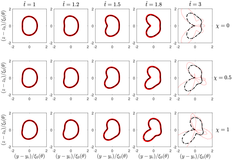
Equation (92) should match the analytical solution (29). Therefore, values of and can be readily determined, and they are written in Table 1. Figure 13 shows predictions of the wake shape based on both the analytical and empirical solutions for different values of dimensionless time and rotation rate . As expected, the empirical relation provides similar results to those of the analytical solution at small values of . Moreover, unlike the analytical solution, it provides reasonable predictions for large values of (i.e., ).
Appendix C Large Eddy Simulation code
The numerical code used in this study is the pseudo-spectral large-eddy simulation code LESGO. It solves the filtered Navier-Stokes equations in rotational form
| (93) | |||
| (94) |
where is the filtered velocity field, is the subgrid stress tensor, is the modified pressure, is the driving streamwise pressure gradient, and are the turbine forces. The subgrid stress tensor is defined using an eddy viscosity model
| (95) |
where is the filtered strain rate tensor. LESGO simulates Cartesian domains using a psuedo-spectral numerical scheme that mixes spectral derivatives in the streamwise direction and spanwise direction with second-order finite-differencing in the vertical direction . Time integration uses the second-order Adams-Bashforth method.
We consider wind turbines under both uniform laminar inflow (Shapiro et al., 2018) and turbulent boundary layer inflows (Shapiro et al., 2020). In the uniform inflow simulations, the Smagorinsky model is used for the eddy viscosity
| (96) |
where is the Smagorinsky coefficient. This choice has a negligible effect on the results as the eddy diffusivity is confined to regions of the flow with strong velocity gradients. The inflow conditions are enforced via a fringe region at the end of the domain. This fringe region smoothly transitions to a prescribed inflow velocity (Stevens et al., 2014). At the top and bottom of the domain, the stress-free boundary conditions for streamwise and spanwise velocity components are applied and the no-penetration condition is applied for the vertical component .
For the turbulent boundary layer simulations, the subgrid stress tensor is modeled using the Lagrangian-averaged scale dependent model (Bou-Zeid et al., 2005). Turbulent inflow conditions are applied using a fringe region forcing where the inflow condition is sampled from a concurrently running simulation (Stevens et al., 2014) with shifted periodic boundary conditions (Munters et al., 2016). At the ground, the stress with a roughness height of is modeled using the equilibrium wall model. The total wall stress is given by
| (97) |
where is the vertical grid spacing, is the von-Kármán constant, and is the velocity magnitude . The wall stress is then apportioned to each component as
| (98) |
LESGO implements the actuator disk model with rotation (ADM-R) using the local formulation for the thrust and angular forces. The thrust force in this forumulation is
| (99) |
where is the local thrust coefficient and is the disk averaged velocity. The total thrust force is distributed across the swept area of the disk using the filtered indicator function
| (100) |
in the unit normal direction to the disk . The filtered indicator function is found by convolving
| (101) |
an indicator function for the geometric shape of the disk with finite thickness with a Gaussian filtering kernel with a characteristic width that is proportional to the mean grid size .
To define the angular force of the rotation actuator disk in a local formulation, we consider the actuator disk model for unyawed wind turbines. The disk-averaged velocity , streamwise velocity deficit , and angular change in velocity are defined based on the streamwise and tangential induction factors and rotation rate of the disk . Considering annular rings of the swept area of the rotor, the annular thrust is the product of the annular flow rate and the change in momentum . The annular torque is similarly the product of the annular flow rate and the change in angular momentum .
Since the annular power is equal to the products and , the following equality
| (102) |
can be solved for the tangential induction factor, so we obtain
| (103) |
The torque can be written in local and standard forms
| (104) |
Defining the tip speed ratio and local tip speed ratio as the torque coefficient is
| (105) |
For ideal actuator disks . The tangential force is then found from
| (106) |
The tangential force applied by the rotating rotor in LESGO is written as
| (107) |
where is the tangential unit vector. In the case of no wake rotation, the tip speed ratio is infinite and the angular force vanishes.
References
- Ablowitz & Fokas (2003) Ablowitz, M.J. & Fokas, A.S. 2003 Complex variables: introduction and applications. Cambridge University Press.
- Anderson (2011) Anderson, J.D. 2011 Fundamentals of aerodynamics. McGraw-Hill.
- Bartl et al. (2018) Bartl, J., Mühle, F., Schottler, J., Sætran, L., Peinke, J., Adaramola, M. & Hölling, M. 2018 Wind tunnel experiments on wind turbine wakes in yaw: Effects of inflow turbulence and shear. Wind Energy Science Discussions 2018, 1–22.
- Bastankhah & Porté-Agel (2014) Bastankhah, M. & Porté-Agel, F. 2014 A new analytical model for wind-turbine wakes. Renewable Energy 70, 116–123.
- Bastankhah & Porté-Agel (2015) Bastankhah, M. & Porté-Agel, F. 2015 A wind-tunnel investigation of wind-turbine wakes in yawed conditions. In Journal of Physics: Conference Series, , vol. 625, p. 012014. IOP Publishing.
- Bastankhah & Porté-Agel (2016) Bastankhah, M. & Porté-Agel, F. 2016 Experimental and theoretical study of wind turbine wakes in yawed conditions. Journal of Fluid Mechanics 806, 506–541.
- Bastankhah & Porté-Agel (2019) Bastankhah, M. & Porté-Agel, F. 2019 Wind farm power optimization via yaw angle control: A wind tunnel study. Journal of Renewable and Sustainable Energy 11 (2), 023301.
- Bastankhah et al. (2020) Bastankhah, M., Welch, B.L., Martínez-Tossas, L.A., King, J. & Fleming, P. 2020 Analytical solution for the cumulative wake of wind turbines in wind farms. arXiv preprint arXiv:2011.00894 .
- Blondel & Cathelain (2020) Blondel, F. & Cathelain, M. 2020 An alternative form of the super-gaussian wind turbine wake model. Wind Energy Science Discussions 2020, 1–16.
- Blondel et al. (2020) Blondel, Frèdèric, Cathelain, Marie, Joulin, Pierre-Antoine & Bozonnet, Pauline 2020 An adaptation of the super-gaussian wake model for yawed wind turbines. In Journal of Physics: Conference Series, , vol. 1618, p. 062031. IOP Publishing.
- Bossuyt et al. (2021) Bossuyt, J., Scott, R., Ali, N. & Cal, R.B. 2021 Quantification of wake shape modulation and deflection for tilt and yaw misaligned wind turbines. Journal of Fluid Mechanics 917.
- Bou-Zeid et al. (2005) Bou-Zeid, E., Meneveau, C. & Parlange, M. 2005 A scale-dependent Lagrangian dynamic model for large eddy simulation of complex turbulent flows. Phys. Fluids 17 (2), 025105.
- Branlard & Gaunaa (2016) Branlard, E. & Gaunaa, M. 2016 Cylindrical vortex wake model: skewed cylinder, application to yawed or tilted rotors. Wind Energy 19 (2), 345–358.
- Burton et al. (1995) Burton, T., Sharpe, D., Jenkins, N. & Bossanyi, E. 1995 Wind energy handbook, 1st edn. Wiley.
- Calaf et al. (2010) Calaf, M., Meneveau, C. & Meyers, J. 2010 Large eddy simulation study of fully developed wind-turbine array boundary layers. Phys. Fluids 22 (1), 015110.
- Campagnolo et al. (2016) Campagnolo, F., Petrović, V., Schreiber, J., Nanos, E.M., Croce, A. & Bottasso, C.L. 2016 Wind tunnel testing of a closed-loop wake deflection controller for wind farm power maximization. In Journal of Physics: Conference Series, , vol. 753, p. 032006. IOP Publishing.
- Carbajo Fuertes et al. (2018) Carbajo Fuertes, F., Markfort, C.D. & Porté-Agel, F. 2018 Wind turbine wake characterization with nacelle-mounted wind lidars for analytical wake model validation. Remote sensing 10 (5), 668.
- Coelho & Hunt (1989) Coelho, S.L.V. & Hunt, J.C.R. 1989 The dynamics of the near field of strong jets in crossflows. Journal of Fluid Mechanics 200, 95–120.
- Coleman et al. (1945) Coleman, R.P., Feingold, A.M. & Stempin, C.W. 1945 Evaluation of the induced-velocity field of an idealized helicoptor rotor. Tech. Rep.. DTIC Document.
- Fleming et al. (2014) Fleming, P.A., Gebraad, P.M.O., Lee, S., van Wingerden, J., Johnson, K., Churchfield, M., Michalakes, J., Spalart, P. & Moriarty, P. 2014 Evaluating techniques for redirecting turbine wakes using SOWFA. Renewable Energy 70, 211–218.
- Fleming et al. (2019) Fleming, P., King, J., Dykes, K., Simley, E., Roadman, J., Scholbrock, A., Murphy, P., Lundquist, J.K., Moriarty, P., Fleming, K. & others 2019 Initial results from a field campaign of wake steering applied at a commercial wind farm–part 1. Wind Energy Science (Online) 4 (NREL/JA-5000-73991).
- Frandsen et al. (2006) Frandsen, S. T., Barthelmie, R., Pryor, S., Rathmann, O., Larsen, S., Højstrup, J. & Thøgersen, M. 2006 Analytical modelling of wind speed deficit in large offshore wind farms. Wind Energ 9, 39–53.
- Gebraad et al. (2014) Gebraad, P.M.O., Teeuwisse, F.W., Wingerden, J.W., Fleming, P.A., Ruben, S.D., Marden, J.R. & Pao, L.Y. 2014 Wind plant power optimization through yaw control using a parametric model for wake effects – a CFD simulation study. Wind Energy 19, 95–114.
- Howland et al. (2016) Howland, M.F., Bossuyt, J., L.A., Martínez-Tossas, Meyers, J. & Meneveau, C. 2016 Wake structure in actuator disk models of wind turbines in yaw under uniform inflow conditions. Journal of Renewable and Sustainable Energy 8, 043301.
- Howland et al. (2019) Howland, M.F., Lele, S.K. & Dabiri, J.O. 2019 Wind farm power optimization through wake steering. Proceedings of the National Academy of Sciences 116 (29), 14495–14500.
- Jensen (1983) Jensen, N.O. 1983 A note on wind turbine interaction. Tech. Rep. Risø-M-2411. Risoe National Laboratory, Roskilde, Denmark.
- Katić et al. (1986) Katić, I., Højstrup, J. & Jensen, N.O. 1986 A simple model for cluster efficiency. In Proceedings of the European wind energy association conference and exhibition, pp. 407–409. Rome, Italy.
- King et al. (2021) King, J., Fleming, P., King, R., Martínez-Tossas, L. A., Bay, C. J., Mudafort, R. & Simley, E. 2021 Control-oriented model for secondary effects of wake steering. Wind Energy Science 6 (3), 701–714.
- Kleusberg et al. (2020) Kleusberg, E., Schlatter, P. & Henningson, D.S. 2020 Parametric dependencies of the yawed wind-turbine wake development. Wind Energy 23 (6), 1367–1380.
- Lin & Porté-Agel (2019) Lin, M. & Porté-Agel, F. 2019 Large-eddy simulation of yawed wind-turbine wakes: Comparisons with wind tunnel measurements and analytical wake models. Energies 12 (23).
- Mahesh (2013) Mahesh, K. 2013 The interaction of jets with crossflow. Annual review of fluid mechanics 45, 379–407.
- Manwell et al. (2010) Manwell, J.F., McGowan, J.G. & Rogers, A.L. 2010 Wind energy explained: theory, design and application. John Wiley & Sons.
- Martínez-Tossas et al. (2019) Martínez-Tossas, L.A., Annoni, J., Fleming, P.A. & Churchfield, M.J. 2019 The aerodynamics of the curled wake: A simplified model in view of flow control. Wind Energy Science (Online) 4 (NREL/JA-5000-73451).
- Martinez-Tossas & Branlard (2020) Martinez-Tossas, L.A. & Branlard, E. 2020 The curled wake model: equivalence of shed vorticity models. J. Phys.: Conf. Ser. 1452, 012069.
- Martínez-Tossas et al. (2018) Martínez-Tossas, L.A., Churchfield, M.J., Yilmaz, A.E., Sarlak, H., Johnson, P.L., Sørensen, J.N., Meyers, J. & Meneveau, C. 2018 Comparison of four large-eddy simulation research codes and effects of model coefficient and inflow turbulence in actuator-line-based wind turbine modeling. Journal of Renewable and Sustainable Energy 10 (3), 033301.
- Martínez-Tossas et al. (2021) Martínez-Tossas, L.A., King, J., Quon, E., Bay, C. J, Mudafort, R., Hamilton, N., Howland, M.F. & Fleming, P.A. 2021 The curled wake model: A three-dimensional and extremely fast steady-state wake solver for wind plant flows. Wind Energy Science 6 (2), 555–570.
- Marusic et al. (2013) Marusic, I., Monty, J.P., Hultmark, M. & Smits, A.J. 2013 On the logarithmic region in wall turbulence. Journal of Fluid Mechanics 716.
- Meneveau (2019) Meneveau, C. 2019 Big wind power: Seven questions for turbulence research. Journal of Turbulence 20 (1), 2–20.
- Meneveau & Marusic (2013) Meneveau, C. & Marusic, I. 2013 Generalized logarithmic law for high-order moments in turbulent boundary layers. Journal of Fluid Mechanics 719.
- Moore (1978) Moore, D.W. 1978 The equation of motion of a vortex layer of small thickness. Studies in Applied Mathematics 58 (2), 119–140.
- Munters et al. (2016) Munters, W., Meneveau, C. & Meyers, J. 2016 Shifted periodic boundary conditions for simulations of wall-bounded turbulent flows. Phys. Fluids 28 (2), 025112.
- Niayifar & Porté-Agel (2016) Niayifar, A. & Porté-Agel, F. 2016 Analytical modeling of wind farms: A new approach for power prediction. Energies 9 (9), 741.
- Okulov & Sørensen (2010) Okulov, V.L. & Sørensen, J.N. 2010 Maximum efficiency of wind turbine rotors using joukowsky and betz approaches. Journal of Fluid Mechanics 649, 497.
- Okulov & Van Kuik (2012) Okulov, V.L. & Van Kuik, G.A.M. 2012 The betz–joukowsky limit: on the contribution to rotor aerodynamics by the british, german and russian scientific schools. Wind Energy 15 (2), 335–344.
- Park & Law (2016) Park, Jinkyoo & Law, Kincho H 2016 A data-driven, cooperative wind farm control to maximize the total power production. Applied Energy 165, 151–165.
- Porté-Agel et al. (2020) Porté-Agel, F., Bastankhah, M. & Shamsoddin, S. 2020 Wind-turbine and wind-farm flows: a review. Boundary-Layer Meteorology 174 (1), 1–59.
- Qian & Ishihara (2018) Qian, G. & Ishihara, T. 2018 A new analytical wake model for yawed wind turbines. Energies 11 (3), 665.
- Rottman et al. (1987) Rottman, J.W., Simpson, J.E. & Stansby, P.K. 1987 The motion of a cylinder of fluid released from rest in a cross-flow. Journal of Fluid Mechanics 177, 307–337.
- Schottler et al. (2017) Schottler, J., Mühle, F., Bartl, J., Peinke, J., Adaramola, M.S., Sætran, L. & Hölling, M. 2017 Comparative study on the wake deflection behind yawed wind turbine models. In Journal of Physics: Conference Series, , vol. 854, p. 012032. IOP Publishing.
- Schreiber et al. (2020) Schreiber, J., Balbaa, A. & Bottasso, C.L. 2020 Brief communication: A double-gaussian wake model. Wind Energy Science 5 (1), 237–244.
- Shapiro et al. (2018) Shapiro, C.R., Gayme, D.F. & Meneveau, C. 2018 Modelling yawed wind turbine wakes: a lifting line approach. Journal of Fluid Mechanics 841.
- Shapiro et al. (2020) Shapiro, C.R., Gayme, D.F. & Meneveau, C. 2020 Generation and decay of counter-rotating vortices downstream of yawed wind turbines in the atmospheric boundary layer. Journal of Fluid Mechanics 903.
- Shapiro et al. (2019) Shapiro, C.R., Starke, G.M., Meneveau, C. & Gayme, D.F. 2019 A wake modeling paradigm for wind farm design and control. Energies 12 (15), 2956.
- Speakman et al. (2021) Speakman, G.A., Abkar, M., Martínez-Tossas, L.A. & Bastankhah, M. 2021 Wake steering of multirotor wind turbines. Wind Energy .
- Stevens et al. (2014) Stevens, R.J.A.M., Graham, J. & Meneveau, C. 2014 A concurrent precursor inflow method for large eddy simulations and applications to finite length wind farms. Renewable Energy 68, 46–50.
- Stevens et al. (2018) Stevens, R.J.A.M., Martínez-Tossas, L.A. & Meneveau, C. 2018 Comparison of wind farm large eddy simulations using actuator disk and actuator line models with wind tunnel experiments. Renew. Energy 116 (Part A), 470 – 478.
- Stevens & Meneveau (2017) Stevens, R.J.A.M. & Meneveau, C. 2017 Flow structure and turbulence in wind farms. Annual review of fluid mechanics 49.
- Van Kuik et al. (2015) Van Kuik, G.A.M., Sørensen, J.N. & Okulov, V.L. 2015 Rotor theories by professor joukowsky: momentum theories. Progress in Aerospace Sciences 73, 1–18.
- VerHulst & Meneveau (2015) VerHulst, C. & Meneveau, C. 2015 Altering kinetic energy entrainment in large eddy simulations of large wind farms using unconventional wind turbine actuator forcing. Energies 8 (1), 370–386.
- Zhan et al. (2020) Zhan, L., Letizia, S. & Iungo, G.V. 2020 Optimal tuning of engineering wake models through lidar measurements. Wind Energy Science 5 (4), 1601–1622.
- Zong & Porté-Agel (2020) Zong, H. & Porté-Agel, F. 2020 A point vortex transportation model for yawed wind turbine wakes. Journal of Fluid Mechanics 890.