Characterising solar surface convection using Doppler measurements

Abstract

The Helioseismic Magnetic Imager (HMI) onboard the Solar Dynamics Observatory (SDO) records line-of-sight Dopplergram images of convective flows on the surface. These images are used to obtain the multi-scale convective spectrum. We design a pipeline to process the raw images to remove large-scale features like differential rotation, meridional circulation, limb shift and imaging artefacts. The Hierarchical Equal Area Pixelization scheme (HEALPix) is used to perform spherical harmonic transforms on the cleaned image. Because we only have access to line-of-sight velocities on half the solar surface, we define a “mixing matrix” to relate the observed and true spectra. This enables the inference of poloidal and toroidal flow spectra in a single step through the inversion of the mixing matrix. Performing inversions on a number of flow profiles, we find that the poloidal flow recovery is most reliable among all the components. We also find that the poloidal spectrum is in qualitative agreement with inferences from Local Correlation Tracking (LCT) of granules. The fraction of power in vertical motions increases as a function of wavenumber and is at 8% level for $\ell=1500$. In contrast to seismic results and LCT, the flows show nearly no temporal-frequency dependence. Poloidal flow power peaks in the range of $\ell-|m|\approx 150-250$ which may potentially hint at a latitudinal preference for convective flows.

1 Introduction

The Sun, like many stars in the main-sequence, possesses a convectively unstable outer envelope surrounding an inner stable core. Given its proximity to us, we observe the Sun with high spatial and temporal resolution. Measurements of plasma flows on the surface reveal a highly intricate and dynamic cellular structure, highlighting a range of spatio-temporal scales (e.g. Miesch, 2005; Rast, 2003). Solar convection, which is primarily driven by buoyancy and radiative cooling at the surface, manifests in an overturning of fluid between the base of the convection zone and the solar surface. Since the fluid is ionized everywhere (almost fully ionized for 97% solar radius and partially ionized in the top 3%; Nordlund et al., 2009), it serves to carry magnetic field, playing a crucial role in setting solar dynamics. Hence, an understanding of solar convection will enable us to better appreciate thermal and angular momentum transport (Aerts et al., 2019), ultimately bringing us closer to explaining the 11-year solar magnetic cycle, a long-standing problem in solar physics.

Solar convection plays out in an extreme parameter regime; the Reynolds number, $Re\sim 10^{14}$, and the Prandtl number, $Pr\sim 10^{-7}$. These regimes are inaccessible to experiments and hence, attempts to understand the physics of turbulent convection of the Sun involve numerical analysis. However, conservative estimates of the viscous dissipation scale of the Sun place it at $\sim 100$ m (Brummell et al., 1995; Lesieur & Metais, 1996), six orders of magnitude smaller than the largest length scale i.e the radius of the Sun, making direct numerical simulation (Orszag, 1970; Moin & Mahesh, 1998) intractable. Hence the inclination to use different types of numerical simulations to study different phenomenon: (a) high-resolution local simulations are used to study dynamics of near-surface layers (Stein & Nordlund, 1998; Rincon et al., 2005) and (b) large-scale flows such as differential rotation are studied using global models based on the anelastic equations (Cattaneo et al., 2003; De Rosa et al., 2002) etc. Simulations attempt to reproduce different aspects of observed solar convection. Hence robust inferences from observational data become a necessity, not only as a standalone measurement by itself, but also as a reference point for validation of numerical simulations.

Observational studies of convection have found three prominent spatial scales. Granulation is a result of vertical advection and downward plume formation driven by radiative losses at the photosphere. Granules are found to occur at spatial scales of $\sim 1$ Mm, with typical lifetimes of $0.2$ hr (Herschel, 1801; Richardson & Schwarzschild, 1950; Leighton et al., 1962). Although mesogranulation was initially observed at a length scale of $\sim 5$ Mm (November et al., 1981; Muller et al., 1992) and a lifetime of $\sim 3$ hours, full-disk observations from HMI have established the absence of peak in convective power at those scales (Hathaway et al., 2015; Rincon et al., 2017). Supergranulation is observed at $\sim 30$ Mm, which advects granular structures (Muller et al., 1992; Rieutord et al., 2010).

Rieutord et al. (2001) showed that granules serve as good tracers of local plasma flows at meso- and supergranular scales over long time scales. Local correlation tracking of granules (November & Simon, 1988) was used to study convection by Georgobiani et al. (2007) in granular to supergranular-scale simulations and they found the velocity spectrum to be approximately a power law for scales larger than granules. Rieutord et al. (2010) studied the high-wavenumber power spectrum using granulation tracking for studying horizontal and vertical velocity by measuring Doppler velocity at disk center. Estimates of the convection spectrum of radial, toroidal and poloidal flows were made by Hathaway et al. (2015) (H15 hereafter) by employing a different method for separately estimating these flows. They noted that the spectrum was dominated by poloidal flows for spherical harmonic degree $\ell>30$ and toroidal flows for $\ell<30$.

The aim of the work is to estimate the vector velocity spectrum on the surface of the Sun, using line-of-sight Dopplergrams. HMI provides us with Dopplergrams measured with a $720$s cadence. Since we measure only the line-of-sight component of velocity on less than half the surface of the Sun, there is a loss of information. Hence, projecting the observed velocities on to any orthonormal basis on the surface of the Sun is imperfect. This is quantified using a mixing-matrix which relates the “true” spectral parameters to their observed counterparts. Previously, Rincon et al. (2017) obtained robust vector velocity spectrum using coherent structure tracking analysis (CST) of granules (Roudier et al., 2012). The uniqueness in our approach is the ability to obtain the toroidal and poloidal (both vertical and horizontal) convection spectrum from the line-of-sight Dopplergrams directly. This enables us to probe the spectral features of the tiniest scales of the observation. The 16 megapixel Dopplergram images from the HMI enable us to obtain spectra upto $\ell$ = 1545. Another novelty of this work is the usage of HEALPix (Górski et al., 2005) for constructing pixels on the solar surface, instead of the traditional Gaussian collocated grid. The Dopplergram images have more pixels near the equator than the poles. Irrespective of longitude, the traditionally used Gaussian collocated grid has the same number of pixels along longitude near the poles and the equator. This results in super-sampling near the poles and under-sampling near the equator. Thus, HEALPix provides us with a natural pixelization on the sphere for solar Dopplergram data.

The outline of the paper is as follows. The theoretical background about spectral decomposition and spectral mixing are dealt with in Section 2. Before applying the present method to HMI data, the raw data need to be cleaned to remove systematical errors, described in Section 3. We discuss corrections due to the motion of HMI in Section 3.1, compensating for gravitational redshift in Section 3.2 and removal of large-scale features in Section 3.3. The analysis of cleaned HMI data is discussed in Section 4. The validation of the inversion procedure is discussed in Section 5. The results are discussed in Section 6.

2 Theoretical Background

The Doppler velocity on the surface $\tilde{\boldsymbol{u}}(\theta,\phi)$ may be expanded in the vector spherical harmonic (VSH) basis $(\boldsymbol{Y}_{\ell m},\boldsymbol{\Psi}_{\ell m},\boldsymbol{\Phi}_{\ell m})$ according as

$$\tilde{\boldsymbol{u}}(\theta,\phi)=\sum_{\ell m}\left(\tilde{u}_{\ell m}\boldsymbol{Y}_{\ell m}(\theta,\phi)+\tilde{v}_{\ell m}\boldsymbol{\Psi}_{\ell m}(\theta,\phi)+\tilde{w}_{\ell m}\boldsymbol{\Phi}_{\ell m}(\theta,\phi)\right).$$ (1)

Definitions and properties of the basis are given in Appendix A. We use both $(\ell,m)$ and $(s,t)$ to denote spherical harmonic degree and the azimuthal order respectively. The $w_{\ell m}$ component is called the toroidal component and $(u_{\ell m},v_{\ell m})$ are together called as the poloidal component. For the sake of differentiating, we would use the term “radial” to refer to the poloidal-vertical component $u_{\ell m}$ and “poloidal” to refer to poloidal-horizontal component $v_{\ell m}$. If we observe all components of velocity on the entire solar surface, then we can perfectly isolate all VSH components $\tilde{U}_{\ell m}=(\tilde{u}_{\ell m},\tilde{v}_{\ell m},\tilde{w}_{\ell m})$, by exploiting the orthonormality of the VSH basis. However, we observe only the velocity projected on to the line-of-sight vector $\hat{\boldsymbol{\ell}}(\theta,\phi)$,

$$\boldsymbol{u}(\theta,\phi)=\left[\hat{\boldsymbol{\ell}}(\theta,\phi)\cdot\tilde{\boldsymbol{u}}(\theta,\phi)\right]\hat{\boldsymbol{\ell}}(\theta,\phi),$$ (2)

over less than half of the solar surface. We use tilde to denote the true spectral components of velocity and to distinguish them from the spectral components of the line-of-sight projected velocity. Hence, observed velocities in spectral domain, $U_{st}=(u_{st},v_{st},w_{st})$ are given by Eqn. (3, 4, 5),

$$u_{st} =\int d\Omega\,W(\theta,\phi)\,\boldsymbol{u}\cdot\boldsymbol{Y}^{*}_{st}$$ (3)

$$v_{st} =\int d\Omega\,W(\theta,\phi)\,\boldsymbol{u}\cdot\boldsymbol{\Psi}^{*}_{st}$$ (4)

$$w_{st} =\int d\Omega\,W(\theta,\phi)\,\boldsymbol{u}\cdot\boldsymbol{\Phi}^{*}_{st},$$ (5)

where $W(\theta,\phi)$ is a window function which has value $1$ where the Sun is observed and $0$ otherwise. Using Eqn. (1), we write the observed spectral components $U_{st}$ in terms of the true spectral components of velocity $\tilde{U}_{\ell m}$,

$$u_{st}=\sum_{\ell}\sum_{m=-\ell}^{\ell}\left(\tilde{u}_{\ell m}M^{(uu)\ell m}_{st}+\tilde{v}_{\ell m}M^{(uv)\ell m}_{st}+\tilde{w}_{\ell m}M^{(uw)\ell m}_{st}\right),$$ (6)

$$v_{st}=\sum_{\ell}\sum_{m=-\ell}^{\ell}\left(\tilde{u}_{\ell m}M^{(vu)\ell m}_{st}+\tilde{v}_{\ell m}M^{(vv)\ell m}_{st}+\tilde{w}_{\ell m}M^{(vw)\ell m}_{st}\right),$$ (7)

$$w_{st}=\sum_{\ell}\sum_{m=-\ell}^{\ell}\left(\tilde{u}_{\ell m}M^{(wu)\ell m}_{st}+\tilde{v}_{\ell m}M^{(wv)\ell m}_{st}+\tilde{w}_{\ell m}M^{(ww)\ell m}_{st}\right).$$ (8)

In Eqns. (6, 7, 8), the matrix $M_{\ell m}^{st}$ quantifies the extent of mixing of true spectral coefficients corresponding to quantum numbers given by $(\ell,m)$ into observed spectral coefficients specified by $(s,t)$. Note that the mixing occurs not only between quantum numbers, but also among the radial, poloidal and toroidal (VSH) components. This is indicated by the superscript parenthesis. For instance, the mixing matrix $M^{(vw)\ell m}_{st}$ quantifies the contribution of the true toroidal component ($w_{st}$) towards the observed poloidal component ($v_{\ell m}$). The mixing matrices are given in Eqn. (9),

$$M^{(ij)\ell m}_{st}=\int d\Omega\,W(\theta,\phi)\,\mathcal{J}^{(ij)}_{\ell m}\mathcal{K}^{(ij)*}_{st},$$ (9)

where $i,j$ are variables which can be any of $u,v,w$. The set of all $\mathcal{J},\mathcal{K}$ are given in Table (1)

Table 1: Table of $\mathcal{J}$ and $\mathcal{K}$

	$i=u$	$i=v$	$i=w$
$j=u$	$\mathcal{J}^{(ij)}_{\ell m}=\hat{\boldsymbol{\ell}}\cdot\boldsymbol{Y}_{\ell m}$; $\mathcal{K}^{(ij)*}_{st}=\hat{\boldsymbol{\ell}}\cdot\boldsymbol{Y}^{*}_{st}$	$\mathcal{J}^{(ij)}_{\ell m}=\hat{\boldsymbol{\ell}}\cdot\boldsymbol{Y}_{\ell m}$; $\mathcal{K}^{(ij)*}_{st}=\hat{\boldsymbol{\ell}}\cdot\boldsymbol{\Psi}^{*}_{st}$	$\mathcal{J}^{(ij)}_{\ell m}=\hat{\boldsymbol{\ell}}\cdot\boldsymbol{Y}_{\ell m}$; $\mathcal{K}^{(ij)*}_{st}=\hat{\boldsymbol{\ell}}\cdot\boldsymbol{\Phi}^{*}_{st}$
$j=v$	$\mathcal{J}^{(ij)}_{\ell m}=\hat{\boldsymbol{\ell}}\cdot\boldsymbol{\Psi}_{\ell m}$; $\mathcal{K}^{(ij)*}_{st}=\hat{\boldsymbol{\ell}}\cdot\boldsymbol{Y}^{*}_{st}$	$\mathcal{J}^{(ij)}_{\ell m}=\hat{\boldsymbol{\ell}}\cdot\boldsymbol{\Psi}_{\ell m}$; $\mathcal{K}^{(ij)*}_{st}=\hat{\boldsymbol{\ell}}\cdot\boldsymbol{\Psi}^{*}_{st}$	$\mathcal{J}^{(ij)}_{\ell m}=\hat{\boldsymbol{\ell}}\cdot\boldsymbol{\Psi}_{\ell m}$; $\mathcal{K}^{(ij)*}_{st}=\hat{\boldsymbol{\ell}}\cdot\boldsymbol{\Phi}^{*}_{st}$
$j=w$	$\mathcal{J}^{(ij)}_{\ell m}=\hat{\boldsymbol{\ell}}\cdot\boldsymbol{\Phi}_{\ell m}$; $\mathcal{K}^{(ij)*}_{st}=\hat{\boldsymbol{\ell}}\cdot\boldsymbol{Y}^{*}_{st}$	$\mathcal{J}^{(ij)}_{\ell m}=\hat{\boldsymbol{\ell}}\cdot\boldsymbol{\Phi}_{\ell m}$; $\mathcal{K}^{*}_{\ell m}=\hat{\boldsymbol{\ell}}\cdot\boldsymbol{\Psi}^{*}_{st}$	$\mathcal{J}^{(ij)}_{\ell m}=\hat{\boldsymbol{\ell}}\cdot\boldsymbol{\Phi}_{\ell m}$; $\mathcal{K}^{(ij)*}_{st}=\hat{\boldsymbol{\ell}}\cdot\boldsymbol{\Phi}^{*}_{st}$

The linear relationships between the observed spectral components $U_{st}$ and the true spectral components $\tilde{U}_{\ell m}$ are given by Eqn. (3 – 5). These relationships may be combined into a single equation by defining vectors $\mathcal{U}$, $\tilde{\mathcal{U}}$ in the following manner,

$$\mathcal{U} =\begin{bmatrix}\,\,\,\ldots\,\,\,u_{i}\,\,v_{i}\,\,w_{i}\,\,\,\ldots\,\,\,\end{bmatrix}^{T}$$ (10)

$$\tilde{\mathcal{U}} =\begin{bmatrix}\,\,\,\ldots\,\,\,\tilde{u}_{i}\,\,\tilde{v}_{i}\,\,\tilde{w}_{i}\,\,\,\ldots\,\,\,\end{bmatrix}^{T},$$ (11)

where $i$ is a combined index denoting the quantum numbers $(\ell,m)$.

$$\begin{bmatrix}\vdots\\ u_{i}\\ v_{i}\\ w_{i}\\ \vdots\end{bmatrix}=\begin{bmatrix}\ddots&\vdots&\vdots&\vdots&\iddots\\ \dots&M^{(uu)j}_{i}&M^{(uv)j}_{i}&M^{(uw)j}_{i}&\dots\\ \dots&M^{(vu)j}_{i}&M^{(vv)j}_{i}&M^{(vw)j}_{i}&\dots\\ \dots&M^{(wu)j}_{i}&M^{(wv)j}_{i}&M^{(ww)j}_{i}&\dots\\ \iddots&\vdots&\vdots&\vdots&\ddots\end{bmatrix}\begin{bmatrix}\vdots\\ \tilde{u}_{j}\\ \tilde{v}_{j}\\ \tilde{w}_{j}\\ \vdots\end{bmatrix},$$ (12)

which may be written in compact form as

$$\mathcal{U}=\mathcal{M}\tilde{\mathcal{U}}.$$ (13)

3 Data Preprocessing

For this study of surface convection, we use line-of-sight Dopplergrams recorded by HMI, which observes the full solar disk at a resolution of 1 arc second (Scherrer et al., 2012). Each Dopplergram is constructed using 72 filtergrams across the Fe-I line (6173.3 $\AA$) at a cadence of 720 seconds. The HMI data pipeline also provides us with a Dopplergram deconvolved with the Point Spread Function (PSF) of the instrument, through the series hmi.V_720s_dConS (1 image per day), which is what we use for this study. The raw image obtained from HMI is shown in Fig. 1.

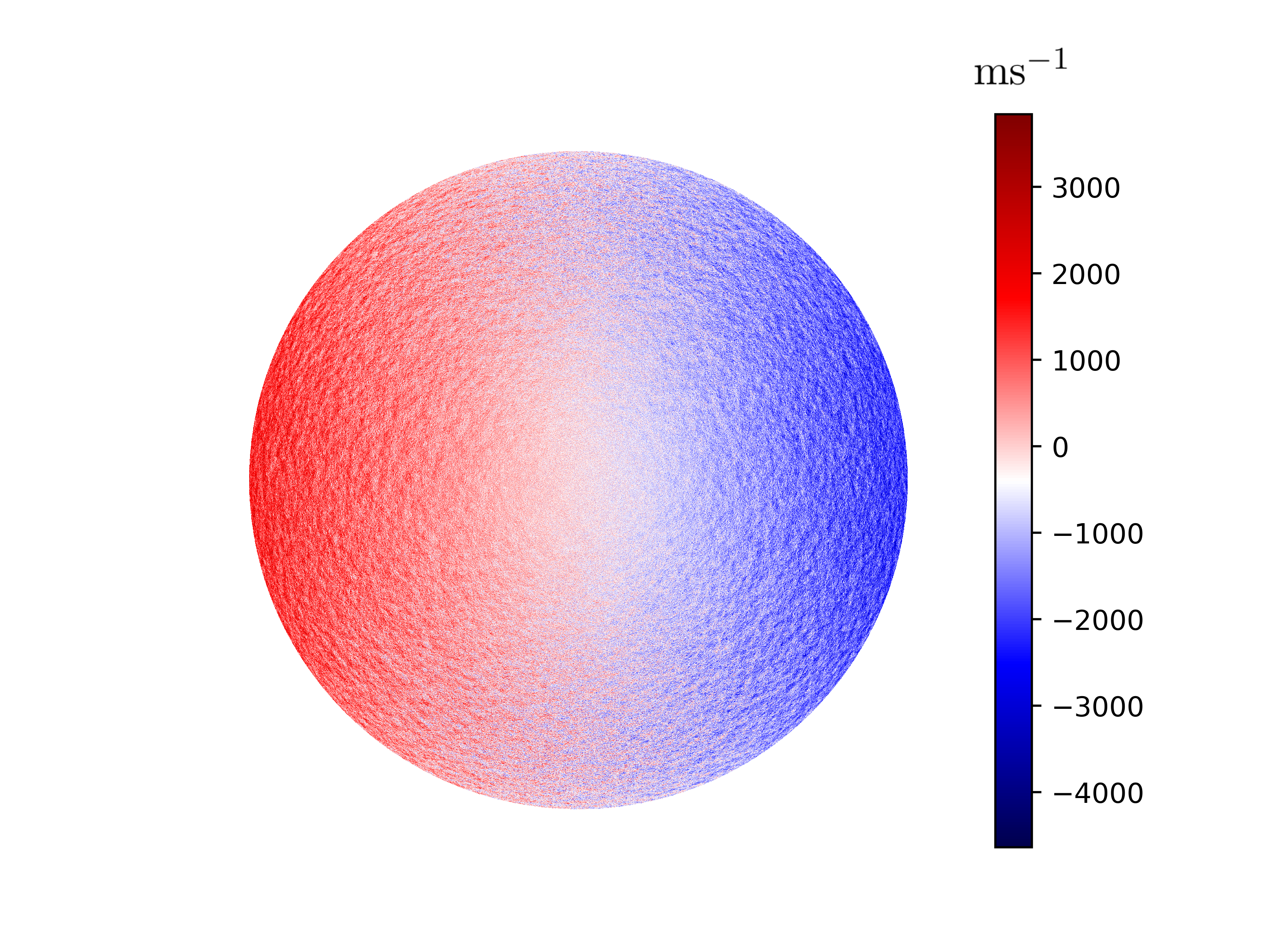
Figure 1: Map of raw Dopplergram after the pixels outside $0.95r_{disk}$ have been removed. The maximum value is $+3840$ ms^-1 and the minimum value is $-4636$ ms^-1

The preprocessing of the raw data involves removal of the following large-scale features which are spurious to the present study:

1. Motion of the observer (HMI).

2. Gravitational redshift.

3. Convective blueshift.

4. Differential rotation.

5. Meriodional circulation.

6. Imaging artefacts.

3.1 Motion of the Observer

The Dopplergram measures the relative velocity between the observer and the source. To measure the velocity on the solar surface in the rest frame of the Sun, the velocity of the spacecraft needs to be accounted for. The HMI data file provides the observer velocity through the keywords OBS_VR, OBS_VN, OBS_VW for velocities in the radial, north-south and east-west directions respectively. In angular heliocentric coordinates, $(\sigma,\chi)$, we write the velocity correction as Eqn. (14),

$$v_{obs}=V_{R}\cos(\sigma)-V_{N}\sin(\sigma)\cos(\chi)-V_{W}\sin(\sigma)\sin(\chi).$$ (14)

This correction is shown over the solar disk in Fig. 2.

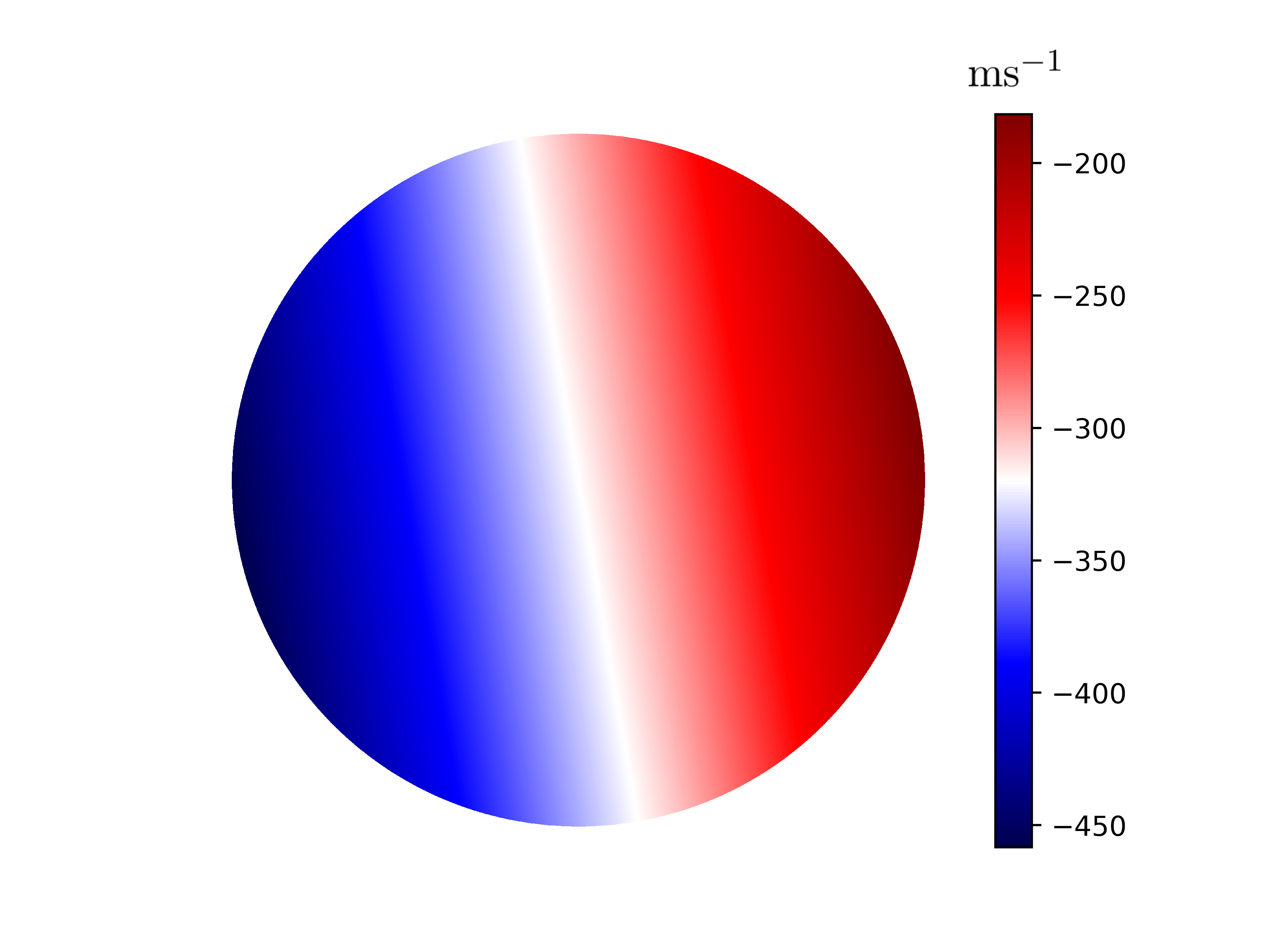
Figure 2: Correction to the Dopplergram due to motion of the observer, in ms^-1. The dominant effect is seen in the east-west direction, as the space-based SDO has the largest component of velocity in the direction of its orbital motion.

3.2 Gravitational Redshift

Gravitational redshift is the consequence of the source (solar surface) being at a higher gravitational potential than the observer (HMI). To leading order, the density profile of the standard solar model (Christensen-Dalsgaard et al., 1996) is spherically symmetric. It was subsequently shown by Basu et al. (1996) that deviations of density from the solar model are at most $1.5$% and the deviations are also a function of only the radius, implying that the gravitational potential is also only a function of radius. Therefore, the surface of the Sun is at the same gravitational potential irrespective of the angular coordinates $(\theta,\phi)$. The redshift computed using Einstein’s principle of equivalence for an observer at infinity is found to be $636$ ms^-1, which is in agreement with observations (Beckers, 1977; Lopresto et al., 1991; Cacciani et al., 2006). The Dopplergram, after removal of contributions due to observer velocity and gravitational redshift, is shown in Figure 3.

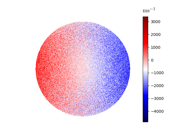
Figure 3: Dopplergram after removal of effects due to motion of the observer and gravitational redshift.

3.3 Convective Blueshift, Differential Rotation and Meridional Circulation

Outside of localized strong magnetic field concentrations, granules dot the entirety of the solar surface. Hot plasma outflows from the cell centers radiate heat and cold plasma plunges into the solar interior through the much narrower intergranular lanes. Hence, at these scales, we would observe a blueshift in the bulk of the granule and redshift at the intergranular lanes. The granules also appear brighter owing to their higher temperatures. Hence, unresolved granules throughout the surface of the solar disk gives rise to an apparent blue shift, which is known as convective blueshift or limb-shift (Beckers & Nelson, 1978; Dravins, 1982). The limb-shift is represented by a polynomial of degree $5$ in heliocentric coordinates (Thompson, 2006).

$$\hat{\boldsymbol{\ell}}\cdot\boldsymbol{u}_{\text{LS}}=\sum_{i=0}^{5}c_{i}P_{i}(x),$$ (15)

where $\boldsymbol{u}_{\text{LS}}$ is the limb-shift, $\hat{\boldsymbol{\ell}}$ is the line-of-sight vector, $x=1-\cos\rho$, $\rho$ being the heliocentric angle and $P_{i}$ are the shifted Legendre polynomials (Appendix B).

Differential rotation is an axisymmetric toroidal component of flow, which is symmetric about the equator. Meridional circulation is an axisymmetric poloidal flow which is antisymmetric about the equator. Hence differential rotation is expressed in terms of the odd-degree toroidal components and meridional circulation using even-degree poloidal components, given by Eqn. (16, 17),

$$\boldsymbol{u}_{\text{DR}}=\sum_{\ell=1,3,5}w_{\ell 0}\,\hat{\boldsymbol{r}}\times\boldsymbol{\nabla}_{h}Y_{\ell 0},$$ (16)

$$\boldsymbol{u}_{\text{MC}}=\sum_{\ell=2,4}v_{\ell 0}\,\boldsymbol{\nabla}_{h}Y_{\ell 0}.$$ (17)

We perform a least-squares fit to estimate the values of $w_{\ell 0}$ and $c_{i}$. The total sum of all three components is shown in Figure 4.

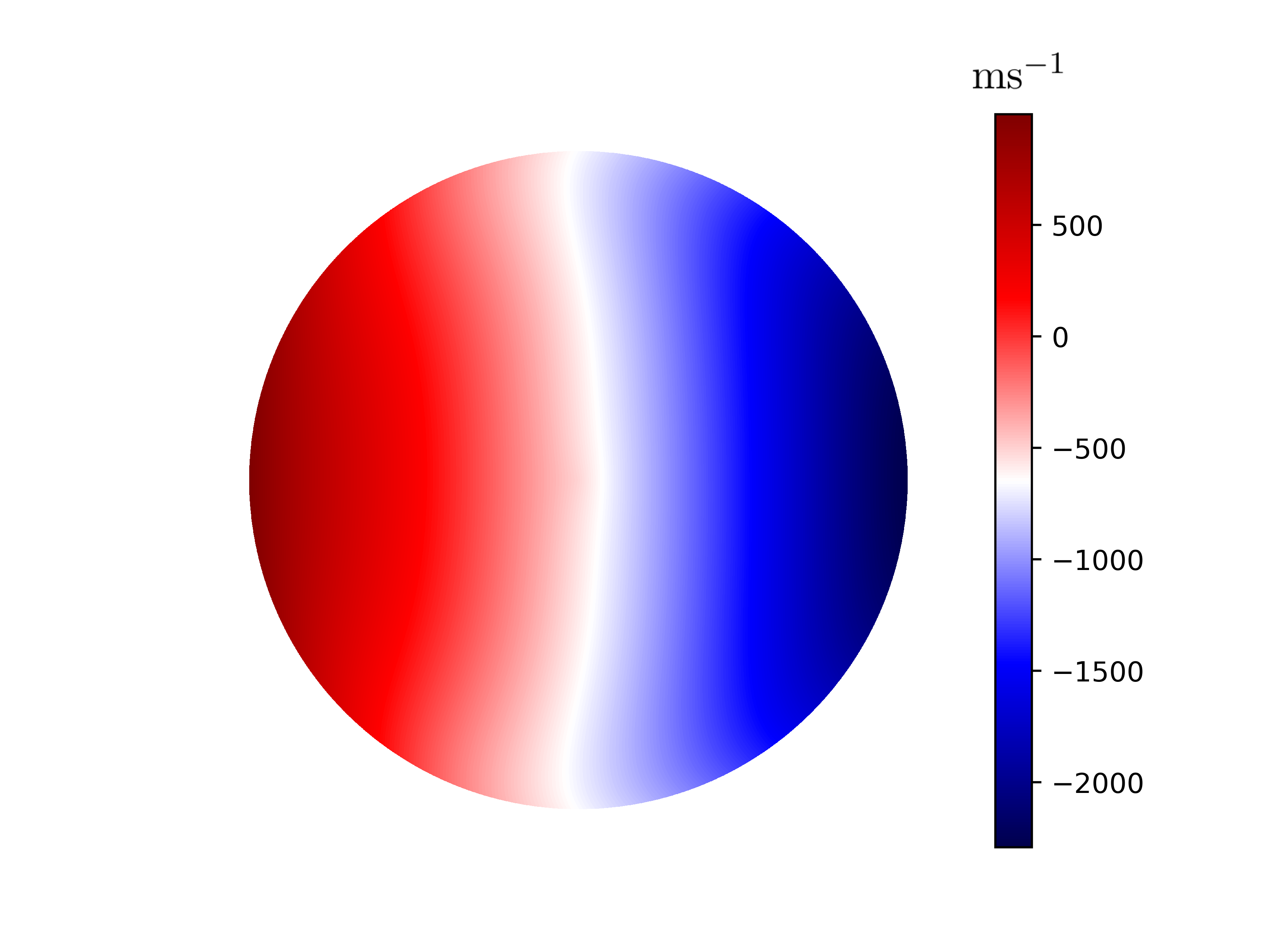
Figure 4: Map showing the combined effect of differential rotation, meridional circulation and convective blueshift. The map has a greater amount of blueshift ($\approx-2500$ ms^-1) than redshift ($\approx 550$ ms^-1) because of the limb-shift correction to be a blueshift all over the solar disk whereas the correction due to differential rotation is red and blue shifted by equal magnitudes.

The final effect that needs to be removed is the imaging artefact. This appears in the form of fringes on the solar disk. We obtain the artefact by averaging over 100 images and subtracting the mean. After removing all these effects, the residual map, shown in Figure 5, is ready for analysis.

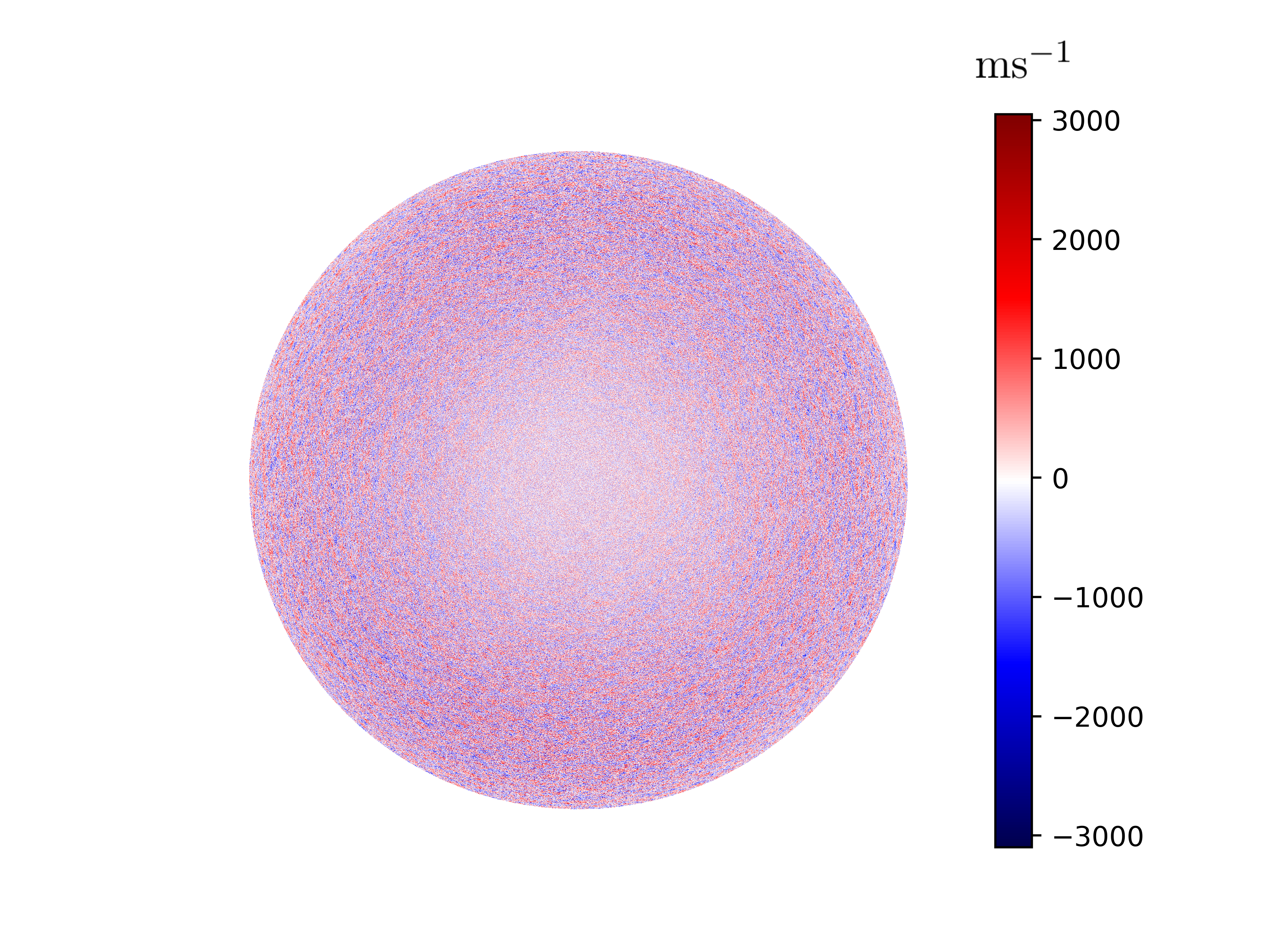
Figure 5: Residual map after the removal of rotation, meridional circulation and limb shift. The disk center is lighter than the limb indicating very low radial velocity component when compared to horizontal velocity.

4 Data Analysis

We perform a spectral analysis on the preprocessed data using the Python package healpy (Zonca et al., 2019). This is based on the HEALPix scheme. The HEALPix scheme divides the surface of a sphere into $N_{\text{pix}}$ pixels of equal area. It also enables an accurate representation of all signals with $\ell\leq\ell_{\text{max}}$, where $\ell_{\text{max}}$ depends on $N_{\text{pix}}$. Each pixel is denoted by its coordinates at its centre. Hence, these pixels are different from grid points on which HMI Dopplergram data are recorded. A schematic overlay of a HEALPix pixel and grid points from HMI is shown in Figure 6. Motivated by radial-velocity measurements of the Sun, which are obtained using the disk-integrated velocity (Wright & Kanodia, 2020), we use an integrated velocity to determine the effective Doppler velocity of the pixel,

$$v^{\text{hp}}A_{\text{pix}}=\int_{A_{\text{pix}}}dA\,\,v^{\text{HMI}}\approx\sum_{i}dA_{i}v_{i}^{\text{HMI}},$$ (18)

where $v^{\text{hp}}$ is the velocity of the HEALPix pixel, $v^{\text{HMI}}$ is the observed velocity from HMI, $A_{\text{pix}}$ is the area of HEALPix pixel and the integration is performed over the region of a HEALPix pixel. Repeating this for each pixel, we obtain a HEALPix map corresponding to the HMI Dopplergram image. This map is used to obtain the observed spectral parameters $(u_{st},v_{st},w_{st})$. The linear relation in Eqn. (13) may be used to determine the “true” spectral parameters $\tilde{\mathcal{U}}$ by inverting mixing-matrix $\mathcal{M}$ in order to compute $\tilde{\mathcal{U}}$. For $\ell_{\text{max}}=1500$, $\mathcal{M}$ has a size $3,377,250\times 3,377,250$. This large matrix may be broken down into a number of smaller dimensional sub-matrices, making the inversions more tractable. The coordinate transformation is shown for $\mathcal{M}^{(uv)\ell m}_{st}$, but it holds for all the sub-matrices given in Table (1). The transformation involves moving the pole to disk-center, which enables integration over the entire domain of the azimuthal coordinate $\phi$. Since all the VSH components are separable functions in $\theta$ and $\phi$, with the dependence on $\phi$ appearing as a phase factor $\exp(im\phi)$, where $m$ is the azimuthal quantum number, the sub-matrices reduce to a function of only the angular degrees $s,\ell$.

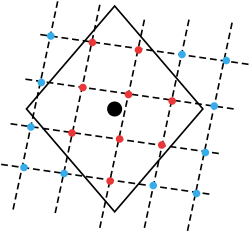
Figure 6: The boundary of a HEALPix pixel is shown in solid line with its coordinates indicated by black dots. The HMI grid points are shown using dashed lines. The grid points which lie within the chosen HEALPix pixel are shown in red and the points which lie outside the pixel are in blue.

$$\mathcal{M}^{(uv)st}_{\ell m} =\int_{0}^{\pi}\sin\theta d\theta W(\theta)\int_{0}^{2\pi}d\phi\,\left(\hat{\boldsymbol{\ell}}\cdot\boldsymbol{\Psi}_{st}\right)\left(\hat{\boldsymbol{\ell}}\cdot\boldsymbol{Y}^{*}_{\ell m}\right)$$

$$=\int_{0}^{\pi}\sin\theta\,d\theta\,W(\theta)f^{s}_{\ell}(\theta)\,\int_{0}^{2\pi}d\phi\exp(i(m-t)\phi)$$

$$=\delta_{m}^{t}\int_{0}^{\pi}\sin\theta\,d\theta\,W(\theta)\,f_{\ell}^{s}(\theta),$$ (19)

where $f_{\ell}^{s}(\theta)$ is the $\theta$-dependent part of $\left(\hat{\boldsymbol{\ell}}\cdot\boldsymbol{\Psi}_{\ell m}\right)\left(\hat{\boldsymbol{\ell}}\cdot\boldsymbol{Y}^{*}_{st}\right)$. It is seen that, in this coordinate system, there is no mixing between different azimuthal quantum numbers. Hence, we may separate the linear equation given by Eqn. (13) into independent equations for each $0\leq m\leq\ell_{\text{max}}$. Since the mixing atrices for each azimuthal order are independent of each other, their inverses are computed in a parallel fashion by using GNU Parallel by Tange (2018). These matrices have very large null spaces; the mixing-matrices transform the true spectral parameters in to the observed spectral parameters and hence there is a loss of information due to observing only the line-of-sight component of half the solar surface.

The regularized inverse is computed by using unit regularization.

$$\tilde{\mathcal{U}}=\left(\mathcal{M}^{T}\mathcal{M}+\lambda I\right)^{-1}\mathcal{M}^{T}\mathcal{U},$$ (20)

where $\lambda$ is the regularization parameter.

A similar analysis by Rincon et al. (2017) employed CST to obtain the velocity spectrum. At the outset, we note that CST generates robust estimates of horizontal velocities. However, since the velocity is measured by tracking granular structures, the spectrum is limited to $\ell<850$, whereas the current work allows us to image up to $\ell=1535$. The current work can be extended to even higher $\ell$, provided sufficiently resolved observations are available.

5 Goodness of inversion

The mixing matrix $\mathcal{M}$ transforms the complete velocity spectrum on the entire surface of the Sun to the line-of-sight spectrum on less than half the solar surface. Hence, $\mathcal{M}$ has a large null-space; the observed spectrum is insensitive to (a) components of velocity perpendicular to the line of sight, and (b) all components of velocity on the farside of the Sun. To understand how well the inversion is able to reproduce the true spectra, we construct a variety of qualitatively different synthetic spectra given below.

For sake of illustration, only synthetic tests for sectoral harmonics are shown in Figure 7. It is seen that the inversion of the poloidal component is the most accurate. Inverted values of radial and toroidal components are seen to follow the same power law, but differ in magnitude when compared to the true spectrum. The inversion tests for all the other cases are presented in Appendix C. Across all the synthetic profiles, the inversion of the poloidal component seems to be accurate and hence robust. It is also observed that the inverted spectra of all flow components are systematically underestimated in the synthetic tests.

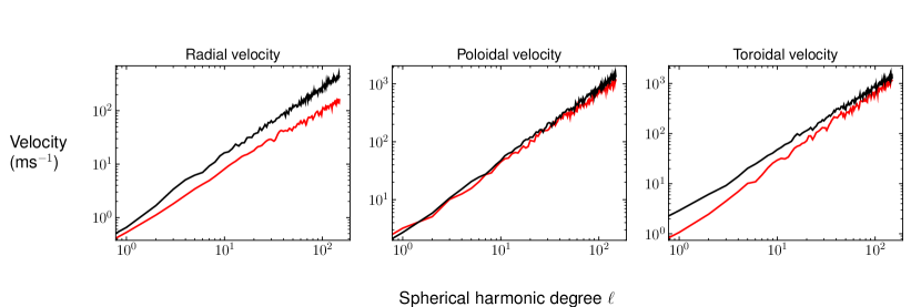
Figure 7: Comparison of actual (black) and inverted (red) velocity profiles for sectorally dominated synthetic spectra. The poloidal spectrum reproduction is significantly superior to the radial and toroidal spectra.

6 Results and Discussion

The HEALPix method involves constructing and heirarchically subdividing the entire spherical surface. The number of subdivisions is denoted by $n_{d}$ and the corresponding number of HEALPix pixels is given by $12\times 4^{n_{d}}$, i.e., $n_{d}=0$ corresponds to the largest pixels where the sphere is equally divided into 12 pixels. All subsequent refinement in pixel size involves dividing cells into 4 sub-divided cells and hence the number of pixels $N_{\text{pix}}=\{12,48,192...\}$. Mapping the observed HMI Dopplergram to HEALPix involves populating the pixels with observed data. Using a very high resolution would result in a lot of “holes” in the remapped data. This happens when the pixel size using HEALPix is smaller than the existing grid. A very low resolution would result in loss of information at smaller spatial scales and hence not preferred. For the 16 megapixel data from HMI, it was found that the optimal $n_{d}=9$ ($N_{\text{side}}=512$ in HEALPix terminology). For this resolution, HEALPix may accurately represent band-limited signals up to spherical harmonic degree $\ell=1535$. HEALPix also enables faster computation of spectrum as the computation of spherical harmonic transform scales as $\mathcal{O}(N_{\text{pix}}^{1/2})$, thus making it attractive for processing of high-resolution data.

The mixing matrix is constructed for all $m\leq 1535$ and inversion is performed to obtain the full spectrum. We compare the results of inversion from forward modelling of H15 and spectrum obtained from LCT in Figure 8. Supergranules have finite depth extents and are sensitive to flows at a range of sub-surface layers. The estimates of flow velocities that LCT (which uses supergranular motions) provides are thus likely to be different from those derived using Dopplergrams because the depth averaging in these two measurements is different. We would thus expect qualitative and approximate quantitative agreement between the two techniques.

While H15 estimates spectra for $\ell\leq 4096$, the current work is limited to $\ell\leq 1535$ and LCT is limited to $\ell\leq 383$. The poloidal flow shows a clear peak at $\ell\approx 120$ which is the well known peak of supergranulation. This peak is seen in the spectrum obtained from LCT as well as H15. Note that, although LCT and H15 are in good agreement over the range $60\lessapprox\ell\lessapprox 120$, they qualitatively differ for $\ell\lessapprox 60$. On the other hand, inferences from the current work are in good qualitative agreement with LCT, but the magnitudes are different.

As evident from the synthetic tests, the magnitude is an underestimate of the true convective amplitudes. Since supergranulation is dominantly poloidal, the peak near $\ell=120$ should appear only in the radial and poloidal components. However, it is seen that the supergranulation peak appears in the toroidal flow inversion as well. This is due to mode mixing and the inability of the inversion to completely separate out the poloidal from the toroidal component. The ability of the inversion to distinguish between the magnitudes of radial and poloidal flows hints at limited contamination of radial flows by poloidal flows.

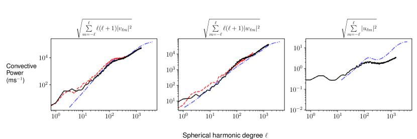
Figure 8: Comparison of convective power spectrum from 3 different methods. The present work is indicated by solid black line. The spectrum obtain from LCT is shown as a dashed red line. The spectrum from H15 is shown in dash-dotted blue line. The present work agrees with inferences from LCT better than H15 for poloidal flow. LCT measures only horizontal velocity and hence the radial flow comparison is with H15 only.

Radial power increases with angular degree, with spatial scales near granulation having the highest power, since granulation comprises strong upflows and downflows. The magnitude of the radial component is also underestimated when compared with H15, although the fractional radial convective power is in good agreement with previous studies (Hathaway et al., 2002, 2015). As shown in Figure 9, at lower $\ell$, the radial power only corresponds to $5\%$ of the total power and at $\ell\approx 1500$, it contributes almost $8\%$. The peak radial velocity at supergranular scales is found to be 2.2 ms^-1, which is an underestimate when compared to T. L. Duvall & Birch (2010) (4 ms^-1), Hathaway et al. (2002) (13 ms^-1) and measurement of 20 ms^-1 by Rincon et al. (2017). It is also within the upper limit of 10 ms^-1 set by Giovanelli (1980).

Figure 9: Fraction of total power contained in radial component as a function of spherical harmonic degree. The fraction increases with wavenumber. A supergranular peak at around $s=120$ is also seen here, hinting at its convective origin. Although the peak could be due to the contamination from the poloidal power, synthetic tests show that contamination is minimal (Appendix E). The radial flow magnitude agrees more with the measurement of vertical RMS velocity T. L. Duvall & Birch (2010) than other measurements.

To study the temporal characterisitcs of the inverted convective flow spectra, we process 1 year’s worth of data at a rate of 1 image per day, with a maximum (Nyquist) frequency of $5.6\,\mu$ Hz and a frequency bin size of $31.7$ nHz. We compute the convective power in all the convective flow components, as a function of spherical harmonic degree $\ell$ and temporal frequency $\nu$. However, the contour plot of $\ell-\nu$ is not informative, i.e., we do not observe clear characteristic frequencies in radial, poloidal or toroidal flow components. Other studies of convection have observed supergranular waves which are found to have oscillation periods of $\sim 2$ $\mu$Hz (Gizon et al., 2003; Langfellner et al., 2018). Additionally Hanasoge et al. (2020) estimated that the toroidal flow power increased significantly with temporal frequency.

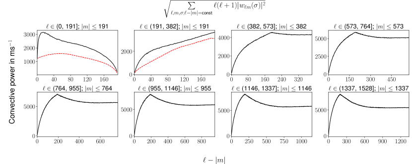
Figure 13: Distribution of toroidal flow power as inferred from LCT (red) and the current work (black). The profiles from inversion peak at low $\ell-|m|$ whereas LCT data attain their maximum at intermediate $\ell-|m|$.

Inversions for the full spectrum enable us to characterise the shapes of convection at different length scales. Sectoral harmonics show power concentrated at low latitudes. Tesseral harmonics have power distributed across the entire surface and zonal harmonics have axisymmetric structure. This classification can be quantified using $\ell-|m|$, which quantifies the number of nodes in latitude. We plot the distribution of power as a function of $\ell-|m|$ for poloidal flows in Figure 10 and for toroidal flows in Figure 11. Irrespective of the range of $\ell$, we observe that the poloidal convective power is maximum for low $\ell-|m|$ i.e. sectoral harmonics. This is also seen to be in qualitative agreement with LCT data, as seen in Figure 13, except at very low $\ell-|m|$. A more detailed comparison is presented in Figs. (19, 21) of Appendix D.

Solar differential rotation is known to have conical (as opposed to cylindrical) isorotation contours inside the convection zone (Gilman & Howe, 2003). Theoretical modelling (Balbus et al., 2009) suggests that a latitudinal temperature gradient is necessary both in the convection zone and at the tachocline to sustain the observed rotational shear. Non-cylindrical differential rotation is driven by a combination of Reynolds stresses and a latitudinal temperature gradient (Miesch, 2005). Measurements of surface temperatures have shown latitudinal variations of a few K (Kuhn et al., 1998; Rast et al., 2008) with a minimum at mid-latitudes. A temperature minimum at mid-latitudes also hints at preferred latitudes for convection and could potentially be the reason for the peak at finite $\ell-|m|$ seen in the poloidal flows shown in Figure 12.

Seismic analyses by Hanasoge et al. (2020) indicate that toroidal power peaks at the equator and is very small beyond $\ell-|m|>10$, for $\ell<50$. Our inversions here for toroidal flow power attain a maximum around $\ell-|m|\sim 20$ (Figure 11) whereas LCT data shows a dominant peak at $\ell-|m|\sim 100$. However, given the poor reproduction of toroidal spectrum in the synthetic tests, the results of inverted toroidal flows are not reliable.

Understanding the origin of supergranulation has been a long-standing challenge (Rieutord et al., 2010). ‘Realistic’ numerical simulations (which account for ionization and radiative transfer) have been successful at reproducing granular scales (Stein & Nordlund, 1998). While Rast (2003) attributed supergranulation to be emergent from advective interaction of granular plumes, attempts at simulations at these scales have been made through two different approaches (a) global spherical simulations where supergranulation corresonds to the smallest scale (e.g De Rosa et al., 2002) and (b) local cartesian simulations where supergranulation is the largest scale (e.g. Cattaneo et al., 2001). Schrijver et al. (1997) suggested that granular and supergranular have very similar features (after accounting for length-scale differences); the real utility in inversion-based observational studies such as the present is that it provides full spectral information of flows at these scales, useful for potentially detecting trends and benchmarking numerical simulations and seismic analyses.

Experimental studies of forced rotating turbulence have shown the presence of a double turbulent cascade – a direct cascade at smaller scales and an inverse cascade at larger scales (Campagne et al., 2014). This is similar to observed convective power around the the supergranular length scales. While Rincon et al. (2017) observe an $\ell^{2}$ scaling for convective poloidal power for $\ell<120$, we find that the scaling to be closer to $\ell^{4}$, which is observed in homogeneous turbulence Batchelor & Proudman (1956); solar convection is known to be neither homogeneous nor isotropic (owing to unstable stratification; Rincon, 2007). However, the large null-space of the mixing-matrix prevents us from quantifying the uncertainties in the inferred spectra and hence we are cautious about drawing detailed conclusions from these measurements. The ratio of toroidal and poloidal flow power can be used to identify the regime of turbulence that the Sun operates in (Horn & Shishkina, 2015, experiments on Rayleigh-Bernard convection), and the present work enables the characterization of the horizontal flows at very high $\ell$. The convective flow power is found to flatten out at higher angular degrees near the granular length scales, and the present work would also be useful for the study of convection at sub-granular length scales, when higher resolution observations become available.

Some of the results in this paper have been derived using the healpy and HEALPix packages. SGK thanks Pranav Sampathkumar (Karlsruhe Institute of Technology) for help with HEALPix. LCT data was generated by Bjoern Loeptien (Max Planck Institute for Solar System Research) and provided by the authors of Hanson et al. (2020). SMH thanks R. Bogart (Stanford University) and D. Hathaway (NASA Ames) for useful conversation. The authors thank Aimee Norton (Stanford Univeristy) for help with HMI data. The authors also thank the anonymous referee for valuable suggestions that helped improve the text in this manuscript.

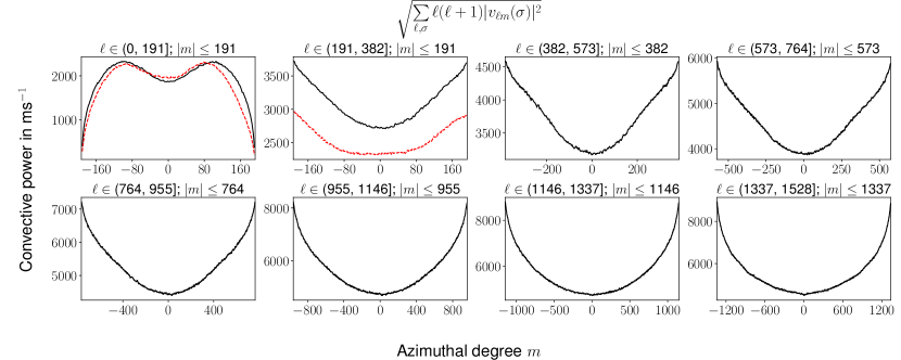
Figure 10: Distribution of poloidal flow power as a function of azimuthal order: LCT data is in red and the present work is shown in black. The power falling at the largest $m$ are due to fewer modes being summed.

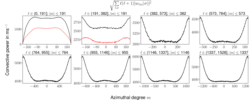
Figure 11: Distribution of toroidal flow power as a function of azimuthal order. LCT data is shown in red and the present work is shown in black. Power declining at the highest $m$ is attributed to fewer modes being summed. LCT and inversion curves are different in both magnitude and trend.

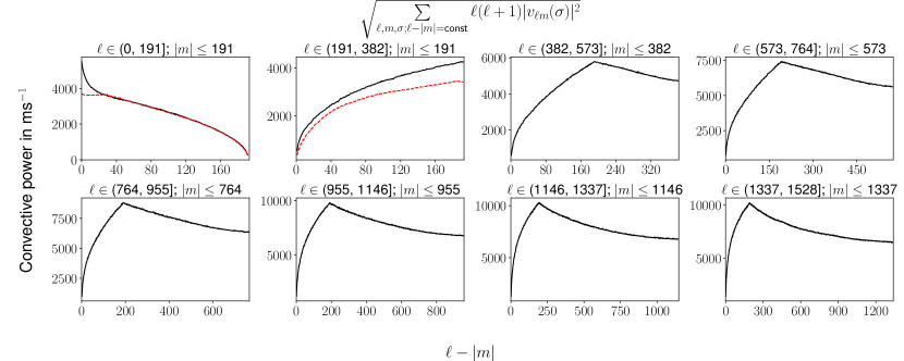
Figure 12: Distribution of toroidal flow power as inferred from LCT (red) and the current work (black). A strong peak is observed for inversions at very low $\ell-|m|$ which isn’t seen in LCT data.

Appendix A Vector Spherical Harmonics

The vector spherical harmonic components are given by

$$\boldsymbol{Y}_{lm}(\theta,\phi) \equiv\hat{\boldsymbol{r}}Y_{lm}(\theta,\phi)$$ (A1)

$$\boldsymbol{\Psi}_{lm}(\theta,\phi) \equiv\boldsymbol{\nabla}_{h}Y_{lm}(\theta,\phi)$$ (A2)

$$\boldsymbol{\Phi}_{lm}(\theta,\phi) \equiv\hat{\boldsymbol{r}}\times\boldsymbol{\nabla}_{h}Y_{lm}(\theta,\phi),$$ (A3)

where $Y_{lm}(\theta,\phi)$ are spherical harmonics and $\hat{\boldsymbol{r}}$ is the radial unit vector and $\boldsymbol{\nabla}_{h}$ is the horizontal gradient operator given by

$$\boldsymbol{\nabla}_{h}=\hat{\theta}\frac{\partial}{\partial\theta}+\hat{\phi}\frac{1}{\sin\theta}\frac{\partial}{\partial\phi}.$$ (A4)

The vector spherical harmonics are orthogonal. The orthonormality may be expressed in compact form if we define $\Lambda^{0}_{lm}\equiv\boldsymbol{Y}_{lm}$, $\Lambda^{1}_{lm}=\boldsymbol{\Psi}_{lm}$ and $\Lambda^{2}_{lm}=\boldsymbol{\Phi}_{lm}$.

$$\int d\Omega\boldsymbol{\Lambda^{i}}_{lm}\cdot\boldsymbol{\Lambda^{j}}^{*}_{l^{\prime}m^{\prime}}=N_{il}\delta^{ij}\delta_{ll^{\prime}}\delta_{mm^{\prime}},$$ (A5)

where $N_{il}$ is a normalization constant, $N_{0l}=1,N_{1l}=N_{2l}=l(l+1)$ and $d\Omega=sin\theta d\theta d\phi$ is the surface element, integration being performed over the entire surface of the Sun.

Appendix B Shifted Legendre Polynomials

The shifted Legendre polynomials are defined over the interval $[0,1]$. In the current computation, we use shifted Legendre polynomials up to degree 5. They are defined as follow,

$$P_{0}(x) =1$$

$$P_{1}(x) =2x-1$$

$$P_{2}(x) =6x^{2}-6x+1$$ (B1)

$$P_{3}(x) =20x^{3}-30x^{2}+12x-1$$

$$P_{4}(x) =70x^{4}-140x^{3}+90x^{2}-20x+1.$$

These polynomials are orthogonal and the orthogonality condition is given by

$$\int_{0}^{1}P_{m}(x)P_{n}(x)=\frac{1}{2n+1}\delta_{mn}.$$ (B2)

Appendix C Inversion – Synthetic Test

The mixing matrix $\mathcal{M}$ needs to be inverted in order to obtain the velocity components on the Sun $U$ from the observed line-of-sight velocity components $\tilde{U}$ as $U=\mathcal{M}^{-1}\tilde{U}$. The mixing matrix $\mathcal{M}$ has a large null space and hence it becomes necessary to perform synthetic tests to establish how well we are able to reproduce different types of spectra.

• Zonal spectra (Figure 14)– the synthetic spectra are non-zero only for $|t|\leq 10$, where $t$ is the azimuthal quantum number.

• Sectoral spectra (Figure 7)– the synthetic spectrum is non-zero only for $s-|t|<10$, where $s$ is the angular degree.

• Tesseral spectra (Figure 15)– the synthetic spectrum is non-zero only for $|t|\geq 10$ and $s-|t|\geq 10$.

• Random spectra (Figure 16)– All spectral components are assigned a random number picked from a uniform distribution.

• Solar-like spectra (Figure 17)– Spectral components where radial components are small compared to horizontal component.

The goodness of inversion is summarized in Table 2. In all the cases, radial and toroidal flows are underestimated. The poloidal flow inversion is the most accurate among the three. Zonal flow inversions are the worst among all the cases, as the inversions capture neither the magnitude of flow nor the power law as a function of wavenumber.

Spectrum type	Radial	Poloidal	Toroidal
Zonal	Underestimate	Good	Bad
Sectoral	Underestimate	Good	Underestimate
Tesseral	Underestimate	Good	Underestimate
Random	Underestimate	Good	Underestimate
Solar-like	Underestimate	Good	Underestimate
Sparse	Underestimate	Good	Underestimate

Table 2: Summary of goodness of spectral reproduction. The poloidal inversion works reasonably well for all kinds of flows.

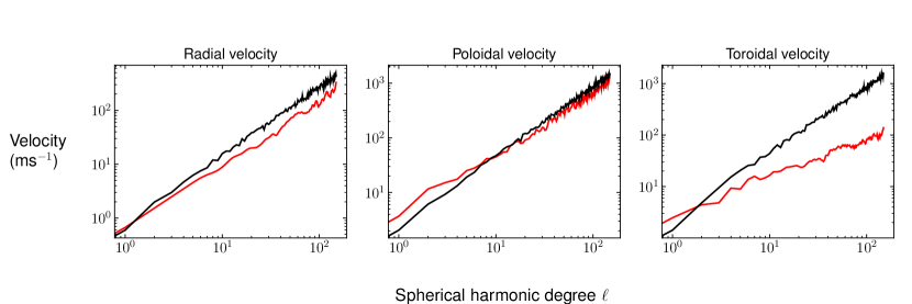
Figure 14: Comparison of actual (black) and inverted (red) velocity profiles for a spectrum with zonal modes. The radial flows show the power law of the synthetic spectrum, but underestimates the magnitude. Poloidal inversion reasonably reproduces the synthetic spectrum for higher $\ell$. Toroidal inversion is erroneous.

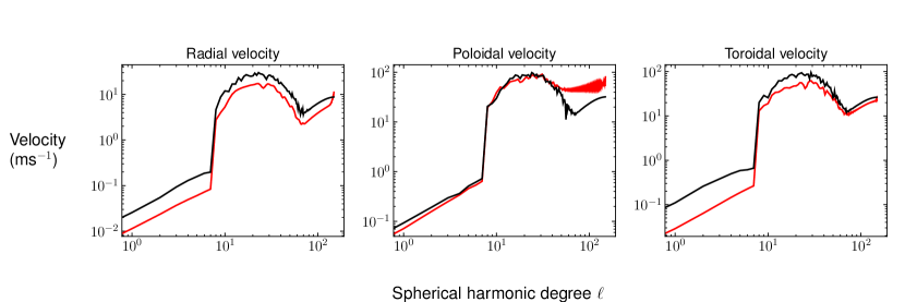
Figure 15: Comparison of actual (black) and inverted (red) velocity profiles for a spectrum with tesseral modes. Radial flows are underestimates of the input synthetic spectrum, whereas poloidal flows are reproduced except at high $\ell$. Toroidal flows are underestimated.

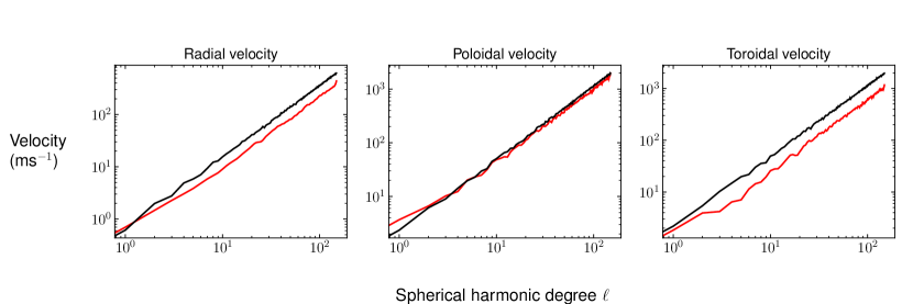
Figure 16: Comparison of actual (black) and inverted (red) velocity profiles for a spectrum with all modes drawn from a uniform random number. Poloidal flows are estimated correctly, whereas radial and toroidal flows are underestimated.

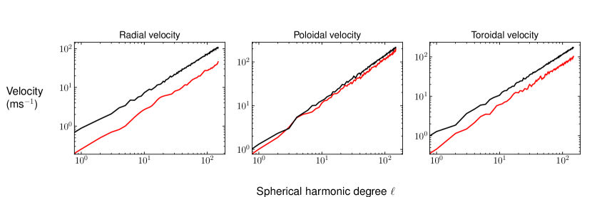
Figure 17: Comparison of actual (black) and inverted (red) velocity profiles for spectrum with solar-like modes. Poloidal flows reproduction are the most accurate among the three. Radial flows are drastically underestimated, and toroidal flows are underestimated as well.

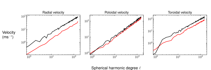
Figure 18: Comparison of actual (black) and inverted (red) velocity profiles for spectrum with sparsely non-zero modes. Poloidal flow inversions work reasonably well. Radial and toroidal flows are underestimated.

Appendix D Comparison with LCT

As demonstrated in Appendix C, the synthetic tests show good poloidal flow reproduction. This can also be seen in the comparison with LCT data as shown in Figs. (19, 20). The toroidal flow inversions are qualitatively different from LCT data as seen in Figs. (21, 22). As the synthetic tests also suggest, toroidal flow inversions are the least trustworthy.

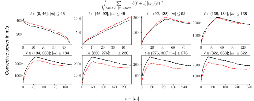
Figure 19: Distribution of poloidal flow power as a function of $\ell-|m|$, inferred from LCT (dashed, red) and the current work (solid, black). LCT indicates a preference for sectoral modes, but the power falls off almost linearly as a function of $\ell-|m|$. Inversions show power concentrated at very low $\ell-|m|$, i.e., the strongest convection at low latitudes.

Figure 20: Distribution of poloidal flow power as a function of azimuthal order $m$, inferred from LCT (dashed, red) and the current work (solid, black). LCT has a pronounced plateau at low $m$. The inversions are in good agreement to LCT up to supergranular wavenumbers.

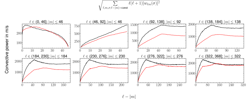
Figure 21: Distribution of toroidal flow power as inferred from LCT (dashed, red) and the current work (solid, black). The inversions underestimate the power and agree qualitatively with LCT up to supergranular wavenumbers. For larger wavenumbers, the LCT spectrum is flat at low $m$.

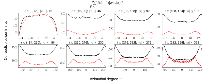
Figure 22: Distribution of toroidal flow power as a function of azimuthal order $m$, inferred from LCT (black) and the current work (red). The LCT power peaks at intermediate $m$ whereas inversions suggest a preference towards extreme $m$.

Appendix E Contamination of radial flows by poloidal flows

To test the contamination of radial flows by poloidal flows, we setup a synthetic test where we perform inversions for 3 different profiles.

1. $(u^{0}_{st},v^{0}_{st},w^{0}_{st})$ - maximum $v^{0}_{st}=240$ ms^-1, maximum $u^{0}_{st}=10$ ms^-1.

2. $(u^{0}_{st},2v^{0}_{st},w^{0}_{st})$ - maximum $v^{0}_{st}=480$ ms^-1, maximum $u^{0}_{st}=10$ ms^-1.

3. $(u^{0}_{st},3v^{0}_{st},w^{0}_{st})$ - maximum $v^{0}_{st}=720$ ms^-1, maximum $u^{0}_{st}=10$ ms^-1.

We plot the error in the inferred $u_{\ell m}$ for cases 2 and 3 relative to the $u_{\ell m}$ of case 1, in Fig 23. For most $\ell$, the error in the estimation of the radial flow is $<10\%$, in spite of the poloidal flow having changed by $200\%$. This shows that the contamination of radial flows by poloidal flows is minimal.

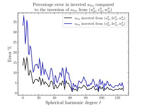
Figure 23: Error in the inference of radial flow when the synthetic poloidal flows are increased by 100% and 200%. It can be seen that the error reduces for higher $\ell$ and is $<10$% for $\ell>20$. The error is also $<5\%$ near the supergranular scales.

References

- Aerts et al. (2019) Aerts, C., Mathis, S., & Rogers, T. M. 2019, ARA&A, 57, 35, doi: 10.1146/annurev-astro-091918-104359
- Balbus et al. (2009) Balbus, S. A., Bonart, J., Latter, H. N., & Weiss, N. O. 2009, MNRAS, 400, 176, doi: 10.1111/j.1365-2966.2009.15464.x
- Basu et al. (1996) Basu, S., Christensen-Dalsgaard, J., Schou, J., Thompson, M. J., & Tomczyk, S. 1996, Bulletin of the Astronomical Society of India, 24, 147
- Batchelor & Proudman (1956) Batchelor, G. K., & Proudman, I. 1956, Philosophical Transactions of the Royal Society of London Series A, 248, 369, doi: 10.1098/rsta.1956.0002
- Beckers (1977) Beckers, J. M. 1977, ApJ, 213, 900, doi: 10.1086/155222
- Beckers & Nelson (1978) Beckers, J. M., & Nelson, G. D. 1978, Sol. Phys., 58, 243, doi: 10.1007/BF00157270
- Brummell et al. (1995) Brummell, N., Cattaneo, F., & Toomre, J. 1995, Science, 269, 1370, doi: 10.1126/science.269.5229.1370
- Cacciani et al. (2006) Cacciani, A., Briguglio, R., Massa, F., & Rapex, P. 2006, Celestial Mechanics and Dynamical Astronomy, 95, 425, doi: 10.1007/s10569-006-9014-0
- Campagne et al. (2014) Campagne, A., Gallet, B., Moisy, F., & Cortet, P.-P. 2014, Physics of Fluids, 26, 125112, doi: 10.1063/1.4904957
- Cattaneo et al. (2003) Cattaneo, F., Emonet, T., & Weiss, N. 2003, ApJ, 588, 1183, doi: 10.1086/374313
- Cattaneo et al. (2001) Cattaneo, F., Lenz, D., & Weiss, N. 2001, ApJ, 563, L91, doi: 10.1086/338355
- Christensen-Dalsgaard et al. (1996) Christensen-Dalsgaard, J., Dappen, W., Ajukov, S. V., et al. 1996, Science, 272, 1286
- De Rosa et al. (2002) De Rosa, M. L., Gilman, P. A., & Toomre, J. 2002, ApJ, 581, 1356, doi: 10.1086/344295
- Dravins (1982) Dravins, D. 1982, ARA&A, 20, 61, doi: 10.1146/annurev.aa.20.090182.000425
- Georgobiani et al. (2007) Georgobiani, D., Zhao, J., Kosovichev, A., et al. 2007, Astrophys. J., 657, 1157, doi: 10.1086/511148
- Gilman & Howe (2003) Gilman, P. A., & Howe, R. 2003, in ESA Special Publication, Vol. 517, GONG+ 2002. Local and Global Helioseismology: the Present and Future, ed. H. Sawaya-Lacoste, 283–285
- Giovanelli (1980) Giovanelli, R. G. 1980, Sol. Phys., 67, 211, doi: 10.1007/BF00149803
- Gizon et al. (2003) Gizon, L., Duvall, T. L., & Schou, J. 2003, Nature, 421, 43, doi: 10.1038/nature01287
- Górski et al. (2005) Górski, K. M., Hivon, E., Banday, A. J., et al. 2005, ApJ, 622, 759, doi: 10.1086/427976
- Hanasoge et al. (2020) Hanasoge, S. M., Hotta, H., & Sreenivasan, K. R. 2020, Science Advances, 6, eaba9639, doi: 10.1126/sciadv.aba9639
- Hanson et al. (2020) Hanson, C. S., Duvall, T. L., Birch, A. C., Gizon, L., & Sreenivasan, K. R. 2020, A&A, 644, A103, doi: 10.1051/0004-6361/202039108
- Hathaway et al. (2002) Hathaway, D. H., Beck, J. G., Han, S., & Raymond, J. 2002, Sol. Phys., 205, 25, doi: 10.1023/A:1013881213279
- Hathaway et al. (2015) Hathaway, D. H., Teil, T., Norton, A. A., & Kitiashvili, I. 2015, ApJ, 811, 105, doi: 10.1088/0004-637X/811/2/105
- Herschel (1801) Herschel, W. 1801, Philosophical Transactions of the Royal Society of London Series I, 91, 265
- Horn & Shishkina (2015) Horn, S., & Shishkina, O. 2015, Journal of Fluid Mechanics, 762, 232, doi: 10.1017/jfm.2014.652
- Kuhn et al. (1998) Kuhn, J. R., Bush, R. I., Scherrer, P., & Scheick, X. 1998, Nature, 392, 155, doi: 10.1038/32361
- Langfellner et al. (2018) Langfellner, J., Birch, A. C., & Gizon, L. 2018, A&A, 617, A97, doi: 10.1051/0004-6361/201732471
- Leighton et al. (1962) Leighton, R. B., Noyes, R. W., & Simon, G. W. 1962, ApJ, 135, 474, doi: 10.1086/147285
- Lesieur & Metais (1996) Lesieur, M., & Metais, O. 1996, Annual Review of Fluid Mechanics, 28, 45, doi: 10.1146/annurev.fl.28.010196.000401
- Lopresto et al. (1991) Lopresto, J. C., Schrader, C., & Pierce, A. K. 1991, ApJ, 376, 757, doi: 10.1086/170323
- Miesch (2005) Miesch, M. S. 2005, Living Reviews in Solar Physics, 2, 1, doi: 10.12942/lrsp-2005-1
- Moin & Mahesh (1998) Moin, P., & Mahesh, K. 1998, Annual Review of Fluid Mechanics, 30, 539, doi: 10.1146/annurev.fluid.30.1.539
- Muller et al. (1992) Muller, R., Auffret, H., Roudier, T., et al. 1992, Nature, 356, 322, doi: 10.1038/356322a0
- Nordlund et al. (2009) Nordlund, Å., Stein, R. F., & Asplund, M. 2009, Living Reviews in Solar Physics, 6, 2, doi: 10.12942/lrsp-2009-2
- November & Simon (1988) November, L. J., & Simon, G. W. 1988, ApJ, 333, 427, doi: 10.1086/166758
- November et al. (1981) November, L. J., Toomre, J., Gebbie, K. B., & Simon, G. W. 1981, ApJ, 245, L123, doi: 10.1086/183539
- Orszag (1970) Orszag, S. A. 1970, Journal of Fluid Mechanics, 41, 363, doi: 10.1017/S0022112070000642
- Rast (2003) Rast, M. P. 2003, ApJ, 597, 1200, doi: 10.1086/381221
- Rast et al. (2008) Rast, M. P., Ortiz, A., & Meisner, R. W. 2008, ApJ, 673, 1209, doi: 10.1086/524655
- Richardson & Schwarzschild (1950) Richardson, R. S., & Schwarzschild, M. 1950, ApJ, 111, 351, doi: 10.1086/145269
- Rieutord et al. (2001) Rieutord, M., Roudier, T., Ludwig, H. G., Nordlund, Å., & Stein, R. 2001, A&A, 377, L14, doi: 10.1051/0004-6361:20011160
- Rieutord et al. (2010) Rieutord, M., Roudier, T., Rincon, F., et al. 2010, A&A, 512, A4, doi: 10.1051/0004-6361/200913303
- Rincon (2007) Rincon, F. 2007, in Convection in Astrophysics, ed. F. Kupka, I. Roxburgh, & K. L. Chan, Vol. 239, 58–63, doi: 10.1017/S1743921307000117
- Rincon et al. (2005) Rincon, F., Lignières, F., & Rieutord, M. 2005, A&A, 430, L57, doi: 10.1051/0004-6361:200400130
- Rincon et al. (2017) Rincon, F., Roudier, T., Schekochihin, A. A., & Rieutord, M. 2017, A&A, 599, A69, doi: 10.1051/0004-6361/201629747
- Roudier et al. (2012) Roudier, T., Rieutord, M., Malherbe, J. M., et al. 2012, A&A, 540, A88, doi: 10.1051/0004-6361/201118678
- Scherrer et al. (2012) Scherrer, P. H., Schou, J., Bush, R. I., et al. 2012, Sol. Phys., 275, 207, doi: 10.1007/s11207-011-9834-2
- Schrijver et al. (1997) Schrijver, C. J., Hagenaar, H. J., & Title, A. M. 1997, ApJ, 475, 328, doi: 10.1086/303528
- Stein & Nordlund (1998) Stein, R. F., & Nordlund, Å. 1998, ApJ, 499, 914, doi: 10.1086/305678
- T. L. Duvall & Birch (2010) T. L. Duvall, J., & Birch, A. C. 2010, The Astrophysical Journal, 725, L47, doi: 10.1088/2041-8205/725/1/l47
- Tange (2018) Tange, O. 2018, GNU Parallel 2018 (Ole Tange), doi: 10.5281/zenodo.1146014
- Thompson (2006) Thompson, W. T. 2006, A&A, 449, 791, doi: 10.1051/0004-6361:20054262
- Wright & Kanodia (2020) Wright, J. T., & Kanodia, S. 2020, The Planetary Science Journal, 1, 38, doi: 10.3847/psj/ababa4
- Zonca et al. (2019) Zonca, A., Singer, L., Lenz, D., et al. 2019, Journal of Open Source Software, 4, 1298, doi: 10.21105/joss.01298