Real-time Monocular Depth Estimation with Sparse Supervision on Mobile

Abstract

Monocular (relative or metric) depth estimation is a critical task for various applications, such as autonomous vehicles, augmented reality and image editing. In recent years, with the increasing availability of mobile devices, accurate and mobile-friendly depth models have gained importance. Increasingly accurate models typically require more computational resources, which inhibits the use of such models on mobile devices. The mobile use case is arguably the most unrestricted one, which requires highly accurate yet mobile-friendly architectures. Therefore, we try to answer the following question: How can we improve a model without adding further complexity (i.e. parameters)?

Towards this end, we systematically explore the design space of a relative depth estimation model from various dimensions and we show, with key design choices and ablation studies, even an existing architecture can reach highly competitive performance to the state of the art, with a fraction of the complexity. Our study spans an in-depth backbone model selection process, knowledge distillation, intermediate predictions, model pruning and loss rebalancing. We show that our model, using only DIW as the supervisory dataset, achieves 0.1156 WHDR on DIW with 2.6M parameters and reaches 37 FPS on a mobile GPU, without pruning or hardware-specific optimization. A pruned version of our model achieves 0.1208 WHDR on DIW with 1M parameters and reaches 44 FPS on a mobile GPU.

1 Introduction

The acquisition of accurate depth information from a scene is an integral part of computer vision, as it provides crucial information of the present 3D structure. This information is imperative to various applications, such as augmented reality, compositing, scene manipulation and robotics. Accurate depth information has traditionally been acquired using multi-camera/stereo setups, LIDARs and other specialized sensors. The use of such sensors in mobile/edge devices may dramatically increase the cost or may not be feasible due to other constraints. Depth estimation using a single camera offers a simpler and a low-cost alternative to such traditional setups.

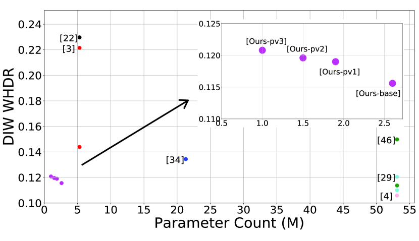
Figure 1: Parameter count vs. DIW WHDR scores. Our models achieve highly competitive results, despite being significantly smaller. Each color represents one method; duplicates of each color represent different results using the same architecture (except the ones denoted by ours). Refer to Table 7 for more details.

Learning-based methods which model the necessary cues for depth estimation have been proposed in [6, 5, 24, 38, 18]. Parallel to these works, instead of predicting metric depth, in-the-wild depth estimation scenarios opted to predict relative depth estimates [47, 46, 3]. Self-supervised methods were also shown to be viable alternatives for monocular depth estimation [7, 8, 14].

The literature primarily focuses on higher accuracy, at the cost of runtime performance and compute requirements, which are not feasible for mobile/edge applications. To address this, lightweight depth estimators have been proposed [44], either by using small backbones or by systematically designing efficient depth estimators. However, such designs have generally been evaluated on restricted cases and not in-the-wild scenarios, which mobile/edge devices operate in.

In this paper, we perform a systematic study and present a detailed pipeline to generate a compact monocular relative depth estimation model. We evaluate and adapt, with key design choices, existing advances in the field, such as knowledge distillation [26], intermediate depth predictions [8], loss rebalancing [20] and pruning [49]. The contributions of our paper are summarized as follows:

• We alter a knowledge distillation pipeline [26] and show that a pixel-wise regression loss, with a suitable teacher network, achieves higher accuracy.

• We augment a loss rebalancing pipeline [20] to work effectively with intermediate prediction layers and show that balancing the decay rate of loss terms and emphasising distillation losses in early training stages help achieve accuracy boosts.

• Our model, despite being 20x smaller than the state-of-the-art and using only DIW as the supervisory dataset, achieves 0.1156 WHDR on DIW and runs at 37 FPS on a mobile GPU. A pruned version of our model, despite being 50x smaller than the state-of-the-art, achieves 0.1208 WHDR and runs at 44 FPS on a mobile GPU.

2 Related Work

2.1 Monocular Depth Estimation

Monocular depth estimation is inherently an ill-posed problem as there is no unique solution (i.e. The same scenes can be projected to the 2D space using non-unique depth maps). Despite this, several cues can be used to restrict the solution space. Using the combination of local predictions [37], semantic-guided predictions [23], non-parametric sampling [15], retrieval [17] and super-pixel optimization [25] methods are examples of such approaches.

Seminal work of Eigen et al. [6] showed a two-stage CNN can learn to infer depth without explicit feature crafting, paving the way for end-to-end solutions for depth estimation. Laina et al. [18] utilized an altered version of ResNet-50 and showed accuracy improvements. Lee et al. [19] showed frequency-domain aggregation of depth map candidates can produce accurate depth maps. Hu et al. [13] showed a feature fusion scheme can improve predictions. Intermediate depth predictions [8], loss rebalancing [20], semantics-driven depth predictions [43], depth estimation with uncertainty [33], attention [48] and geometric constraints [50] have also proven to be viable improvements.

Such advances have been made possible thanks to large datasets with dense depth ground-truths, such as NYUv2 [30], KITTI [5], Mannequin Challenge (MC) [21] and others. Metric depth annotations are, however, quite laborious to obtain, suffer from scale incompabilities and can fail to generalize to unconstrained settings. These problems are partially alleviated by self-supervision, where minimizing a form of reconstruction error using unlabeled monocular sequences is shown to be a viable alternative [7, 8, 14]. A parallel line of work focuses on relative depth estimation, especially for in-the-wild scenarios, by using ordinal ground-truths between pairs of pixels. It was shown that relative depth ground-truth can be used to infer dense or relative depth maps successfully [3]. Several relative depth datasets are proposed [46, 47] to facilitate research in this area.

2.2 Lightweight Models

The advances in depth estimation generally come at the cost of increased computational budgets. For mobile/edge applications, it is imperative to have an accurate model that can perform in real-time in resource-constrained environments. A natural starting point is to replace the backbones of existing models with lightweight alternatives, such as MobileNet [36], GhostNet [9] and Fbnet [45]. Additionally, knowledge distillation [26], reduced precision training and network pruning [49] are common approaches to reduce model size. Several other studies focused on producing efficient depth estimators from scratch, such as feature-pyramid based models [32], low-latency decoder designs [44] and reinforcement-learning based pruning models [42].

A similar work to ours is reported in [2]. Authors compare several lightweight depth estimation models by using a knowledge-distillation based training and perform cross-dataset experiments to assess generalization. Our study differs in several aspects: (1) we present a detailed evaluation and design process for architecture selection, (2) show that a combination of knowledge distillation, (3) intermediate prediction layers and (4) loss rebalancing can achieve competitive results using relative depth ground-truth.

3 Methodology

In this section, we outline our design choices and systematic study to produce an efficient depth estimator.

3.1 Model Design

One of the most critical parts of a machine-learning process is the design of the architecture. We base our model design on U-Net [35] and systematically improve the design by selecting encoder and decoder topologies.

First, we evaluate several encoders while keeping the decoder fixed (except matching the required filter numbers of the encoder) as the one in [44]. We evaluate ShuffleNetv2 [27], MNasNet [39], MobileNetv2 [36], MobileNetv3 [12], EfficientNet [40] variants, MixNet [41], GhostNet [9] and FastDepth [44]. Second, we focus on the decoder design. For the various encoders mentioned above, we compare NNConv5 [44] and an FbNet-based [45] decoder layers.

Our final architecture is based on a MobileNetv2 encoder and an FbNet-based decoder. We observe MobileNetv2 to have a good trade-off between efficiency and accuracy, whereas the FbNet based decoder is smaller and more accurate than the alternatives. We also update the decoder by replacing its last layer with a simple upsampling layer and include five skip connections from encoder to decoder. Our final network architecture is shown in Figure 2.

3.2 Motivation and Baselines

3.2.1 Motivation

Model performance. First, we need to consider the use of mobile depth estimators; they need to work well in arguably the most in-the-wild setting. Increasing the model complexity for a mobile device is generally not an option. Therefore, we need to answer the first question; How can we improve a model’s performance without adding additional complexity? We try to answer this question in Section 3.3

Ground-truth. Second, we need to consider the nature of ground-truth; one may assume metric depth annotations are required for in-the-wild settings. However, depending on the use case, metric depth may not be necessary. In applications such as image relighting and visual effects, we may not need to know the metric depth for each pixel, but knowing their ordering relative to other pixels can be sufficient. Therefore, we need to answer the second question; What type of ground-truth annotations do we want?

Ordinal ground truths, where point-pair relations for one or several points per image are given, are suitable annotations for such scenarios. Relative depth annotations are easier to generate, do not suffer from scale incompatibilities and are more robust to outliers [4]. Moreover, relative depth models can learn strong priors, which can then be projected to any scale in metric depth scenarios. In light of these, we opt to use relative ground-truth annotations.

3.2.2 Baselines

We select datasets that best reflect the in-the-wild case; RedWeb [46], DIW [3] and Mannequin Challenge [21]. The first two have relative ground-truths, which are suitable for our use case. We base our study on performance on DIW, due to several reasons; i) it represents in-the-wild the best due to its size and variance, ii) it is arguably the most suitable datasets for relative depth and iii) its evaluation metrics are the widely used standard for in-the-wild scenarios. Evaluating our improvements requires a baseline, and towards this end, we train our model on each dataset and also sequentially on all of them to serve as a baseline. Next, we formulate the losses used to train our model.

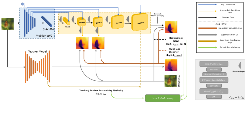
Figure 2: Our architecture and training pipeline. The decoder layers based on FBNet [45] are shown in detail in bottom right. We train our model on DIW ($L_{aux-rk}$ in Eq. (5)) and also distill knowledge [26] from a high-capacity model [4] ($L_{pa}$ and $L_{aux-RMSE}$ in Eq. (5)). During training, we train with intermediate prediction layers which are removed during inference. Our multiple loss terms are balanced during training in real-time [20].

Mannequin Challenge. For training our model on Mannequin Challenge dataset, we use the losses formulated in the original paper [21]. The final loss function consists of three loss terms, which is defined as

$$L_{si}=L_{mse}+a_{1}L_{grad}+a_{2}L_{sm}$$ (1)

where the first term $L_{mse}$ is the scale-invariant mean squared error, the second term $L_{grad}$ is multi-scale gradient term that encourages smoother gradient changes and sharper depth discontinuities in the predictions, the third term $L_{sm}$ is the multi-scale edge-aware smoothness term that encourages smooth interpolation of depth values in textureless regions and $a_{1}/a_{2}$ are loss weights.

DIW. Training on DIW is based on the ranking loss [3], which is defined as

$$\psi_{k}(I,i_{k},j_{k},r_{k},z)=\begin{cases}r_{k}=1,&\log(1+exp(z_{jk}-z_{ik}))\\ r_{k}=-1,&\log(1+exp(z_{ik}-z_{jk}))\\ r_{k}=0,&(z_{ik}-z_{jk})^{2}\end{cases}$$ (2)

where $i_{k}$, $j_{k}$ and $r_{k}$ represent first point, second point and their ground-truth relations for the query $k$ in training image $I$ and $z$ is the predicted depth map. Ground-truth relations are encoded as ${1,-1,0}$ for ordinal relations closer, further and equal, respectively.

RedWeb. Training on RedWeb is done with an improved ranking loss [46], which is defined as

$$\psi_{k}=\begin{cases}l_{k}\neq 0,&\log(1+exp((-z_{ik}+z_{jk})l_{k}))\\ l_{k}=0,&(z_{ik}-z_{jk})^{2}\end{cases}$$ (3)

where $\psi$ is parametrized by input image $I$, $z$ is the estimated depth map, and $i_{j},j_{k},l_{k}$ represent first point, second point and their ordinal relations, respectively.

3.3 Towards a Better Depth Estimator

Now that we have finalized our model design in Section 3.1 and obtained baselines in Section 3.2, we explore ways to improve our model’s accuracy, without adding additional parameters or compute requirements.

Intermediate Predictions. First, we integrate intermediate prediction layers to our model [8, 51], which produce multiple outputs during training. One key difference here is that we remove the intermediate prediction layers after training, and thus preserve the model complexity. The use of intermediate predictions in decoder layers acts as a regularizer and it forces the encoder to learn better representations. We train our network on the combined loss of last and intermediate prediction layers, which is defined as

$$L_{aux}=\sum_{i=1}^{N}{\lambda_{i}L_{i}}$$ (4)

where $L_{i}$ is the loss, $\lambda_{i}$ is the weight term and $i{\in}N$ represents the (intermediate and final) predictions. Our final model has two intermediate prediction layers based on FbNet-like upsampling layers that are used in our decoder. We integrate two intermediate prediction layers after second and third decoder layers and use loss weights $0.5,0.25,0.25$ for the final and intermediate predictions, respectively.

Knowledge Distillation. Second, we use a knowledge distillation mechanism to exploit knowledge learned by larger models. Knowledge distillation is data-efficient method to transfer the knowledge of a large model to a compact model, and leads to accuracy improvements without adding further complexity to the model.

Our knowledge distillation mechanism follows the work of Liu et al. [26], where we use as teacher the EncDecResNet architecture trained on RedWeb, DIW and Y3D datasets [4]. The original knowledge distillation approach formulates three losses to transfer the knowledge to the student; a pixel-wise loss operating on binned depth classes (between student and teacher networks), pair-wise loss operating on feature representations of teacher and student network, and a holistic loss that also trains a discriminator such that the student (i.e. generator) outputs accurate depth maps.

Our implementation differs from the original in several aspects; i) we change the classification-based formulation with simple RMSE for pixel-wise loss, ii) remove holistic loss and iii) use a different teacher network. We select our teacher based on its performance on DIW. We use RMSE for pixel-wise loss since no scale issues are expected (teacher is trained on DIW) and RMSE is one of the strongest supervision available in this scenario. We remove holistic loss since we observe our model reaches its capacity rather quickly, and generator/discriminator pair fail to converge in this time frame. Finally, we heuristically select the feature layers for pair-wise loss and set our student model as the model explained in previous sections, with the additional intermediate prediction layers. Our model is trained with the loss defined as

$$\begin{split}L_{kd}=\lambda_{1}L_{aux^{RMSE}}(S(I),\tau(I))+\lambda_{2}L_{aux^{rk}}(S(I),Y(I))\\ +\lambda_{3}L_{pa}(S(I)_{\ell},\tau(I)_{\ell})\end{split}$$ (5)

where $S$ and $\tau$ are student and teacher networks, $I$ is the training sample, $Y(.)$ is the ground-truth label, $L_{pa}$ is the pairwise loss operating on feature representations $\ell$, and $\lambda$ values are loss weights. We enforce pixelwise ($RMSE$) and ranking loss ($rk$) to every prediction, and enforce pairwise loss between penultimate (decoder) layers of $S$ and $\tau$.

Loss Rebalancing. As can be seen in Equations (4) and (5), there are multiple loss terms driving the model training, which results in another layer of parameter tuning. This is a laborious task as loss values have different value scales and decay rates, which requires periodic scaling of loss weights to facilitate adequate contribution for each loss term.

We alleviate this problem by using automatic loss balancing algorithm proposed in [20]. Authors of the original paper formulate an algorithm that i) performs an initial training stage and records the loss values, ii) scales the values to have a level playing field across loss terms and iii) periodically updates the weights by taking into account the rate of decrease for each loss. The algorithm is a scalable one as it also allows emphasising hard or easy losses first, which are defined so based on the way they decay.

We integrate the said loss rebalancing algorithm with key differences; i) we do not include separate weights for auxiliary layers and keep them wrapped (i.e. $L_{aux}$ shown in Equation (4) has fixed $\lambda$ values), ii) we omit the loss weight initialization/scaling stage and set all weights equal to each other iii) emphasize hard losses first and then easy losses during our training. We do not include separate weights for auxiliary layers because doing so means giving more weights to intermediate losses, which can lead to insufficient supervision for the deeper layers of the decoder. We omit the initial loss weight scaling because we observe that different loss terms have significantly different value scales, and levelling these value scales earlier in the training is likely to degrade the performance. Moreover, we see that focusing on the hard losses first emphasise distillation losses in early training, which essentially is a form of pretraining. We hypothesize this setting is likely to be more beneficial. Essentially, instead of manually choosing $\lambda_{1}$, $\lambda_{2}$ and $\lambda_{3}$ of Equation (5), loss rebalancing adaptively chooses and changes them during training.

Final Words. The final training pipeline is shown in Figure 2. We also prune our model using NetAdapt [49]; we remove the intermediate prediction layers, prune the model and finetune on DIW using the same training pipeline.

4 Experiments

4.1 Experimental Setup

We use PyTorch [31] for training and convert the models to TFLite for performance evaluation [1]. We load ImageNet-pretrained weights for our encoder and initialize the weights using [10] for the decoder.

NYUv2 Depth. [30] includes 48K RGB-D images with a size of 640x480 and the majority of images are in indoor settings. Similar to [44], the model is trained with a batch size of 8 and a starting learning rate of 0.01, which decays by an order of magnitude every 10 epochs. We train for a total of 30 epochs and optimize with SGD, with a momentum of 0.9 and a weight decay of 0.0001. The training is performed with $\ell_{1}$ loss. We use scaling, rotation, color jitter/normalization and random flipping as training augmentations. Augmented data is then resized and center-cropped to 224x224. We use RMSE and $\delta_{1}$ metrics for evaluation. NYUv2 dataset is used in Section 3.1, where the model designs are compared for various encoder/decoder pairs.

Mannequin Challenge. includes 2695 monocular sequences ($\sim$150K frames) with a size of 640x480. Despite its size, since the dataset primarily includes people, its scene distribution is still restricted. The model is trained with a batch size of 16 and a starting learning rate of 0.0004, using the loss function shown in Equation (1). Training is done for 12 epochs with Adam [16] optimiser, where we halve the learning rate every 4th epoch. We use three scales for $L_{sm}$ in Equation (1) and use rotation, color and depth normalization and random flipping as data augmentations. The data is finally resized and then random-cropped to 224x224. We use Scale-Invariant RMSE as the evaluation metric [21]. MC dataset is used in Section 3.2 to create our baselines.

RedWeb. includes 3600 images with dense and relative depth annotations for every pixel in the image [46]. Despite its large scene variance, its size is a limiting factor. The model is trained using a batch size of 4 and a starting learning rate of 0.0004, with the loss function shown in Equation (3). Training is done for 250 epochs with Adam optimizer, where learning rate is halved every 50th epoch. We sample 3000 points for each image randomly and augment the data with rotation, color jitter, color normalization and random flips. The data is resized and random-cropped to 224x224. RedWeb is used in Section 3.2 to create our baselines.

DIW. includes 495K images with relative depth annotations, where a point-pair is sampled per image. DIW is the largest among all others, both in size and distribution. We train using a batch size of 4 and a starting learning rate of 0.0001, with the loss function shown in Equation (2). Training is performed for 5 epochs and Adam optimizer is used, where we halve the learning rate every epoch. The images are resized to 224x448 resolution and then fed to the network. We use WHDR as the evaluation metric [3]. DIW is used in Section 3.2 to create our baselines, as well as in Section 3.3 to train our final depth estimator.

4.2 Model Design

Results for encoder architectures are shown in Table 1, where EfficientNet-based encoders have the best accuracy. In overall, however, MobileNetv2 has the best complexity-accuracy trade-off, therefore it is the best choice available.

Model	RMSE $\downarrow$	$\delta_{1}$ $\uparrow$	Parameters (M)
ShuffleNet v2 [27]	0.615	0.749	2.0
MNasNet [39]	0.608	0.758	4.0
MobileNet v2 [36]	0.583	0.775	3.1
MobileNet v3 [12]	0.607	0.749	5.1
EfficientNet ES [42]	0.572	0.782	5.0
EfficientNet B0 [42]	0.581	0.778	4.9
GhostNet [9]	0.618	0.750	5.4
MixNet M [41]	0.589	0.767	4.5
MixNet S [41]	0.589	0.766	3.6
FastDepth [44]	0.599	0.775	3.9

Table 1: Different encoder architectures’ performance on NYUv2, where decoder is fixed to NNConv5 [44].

Results for decoder architecture comparisons are shown in Table 2. There is a consistent trend regardless of the encoders; FBNet-based decoders outperform NNConv5 decoders while having significantly fewer parameters. Seeing that MNet v2 + FBNet model gives the best parameter/accuracy trade-off, we further remove its last layer of the decoder and replace it with a simple upsampling operation (last row, Table 2) and see that it outperforms the original architecture (penultimate row, Table 2). Our architecture, therefore, is chosen as MNet v2 + FBNetx112 and will be the one used in the following sections.

Model	RMSE $\downarrow$	$\delta_{1}$ $\uparrow$	Parameters (M)
EfNet ES [42] + NNConv5 [44]	0.572	0.782	5.0
EfNet ES [42] + FBNet [45]	0.534	0.802	4.7
MixNet M [41] + NNConv5 [44]	0.589	0.766	4.5
MixNet M [41] + FBNet [45]	0.582	0.773	3.6
GhostNet [9] + NNConv5 [44]	0.618	0.750	5.4
GhostNet [9] + FBNet [45]	0.596	0.756	4.3
MNet v2 [36] + NNConv5 [44]	0.583	0.775	3.1
MNet v2 [36] + FBNet [45]	0.567	0.782	2.6
MNet v2 [36] + FBNet [45] x112	0.564	0.790	2.6

Table 2: Different decoder architectures’ performance on NYUv2. Our model is shown in the last row, which has the best performance/accuracy trade-off.

4.3 Baselines

Our baseline results are shown in Table 3. For NYUv2 and MC, best results are obtained when we train on them, as expected. The second row shows that we achieve 0.1484 WHDR in DIW, if we train on DIW exclusively. When we train on MC, RedWeb and DIW sequentially, we get significant improvements and achieve 0.1316 WHDR. This shows that the distribution of DIW is large and can make use of other datasets with comparably limited data distribution. Our baseline is shown in the last row of Table 3, which is an improved version of the vanilla training on DIW.

Training Dataset	RMSE $\downarrow$	WHDR $\downarrow$	SI-RMSE $\downarrow$
NYUv2	0.564	0.3294	0.3809
DIW	1.332	0.1484	0.4662
RedWeb	1.326	0.2046	0.3973
MC	1.274	0.2401	0.1097
RedWeb $\rightarrow$ DIW	1.319	0.1386	0.4999
MC $\rightarrow$ DIW	1.326	0.1376	0.3973
MC $\rightarrow$ RedWeb $\rightarrow$ DIW	1.313	0.1316	0.4551

Table 3: Our model trained on various datasets. $\rightarrow$ indicates sequential training. The last row shows our baseline.

4.3.1 Ablation Study

We now study the contributions of our design choices; intermediate predictions, knowledge distillation and loss rebalancing. In this section, we perform training only on DIW, but evaluate on all three datasets (MC, RedWeb, DIW).

Intermediate Predictions. We first study the effect of having intermediate prediction layers in our model. We conduct experiments in two training settings to assess intermediate predictions’ usefulness; we train on all three datasets sequentially and also train on DIW with knowledge distillation. For both settings, we show results with one and two intermediate prediction layers, where loss weights are $\lambda_{1}=0.5,\lambda_{2}=0.5$ and $\lambda_{1}=0.5,\lambda_{2}=\lambda_{3}=0.25$ for one and two intermediate prediction layers, respectively. Results are shown in Table 4.

Results show intermediate prediction layers achieve better results across different datasets. Adding one intermediate prediction layer has a degrading effect, but when we add two intermediate prediction layers we get improvements. In sequential training on all our datasets, we get slight loss in WHDR, but achieve improvements in SI-RMSE and RMSE. When trained on DIW with knowledge distillation, we get modest improvements with intermediate prediction on SI-RMSE and WHDR, but lose some accuracy in NYU. In overall, intermediate predictions help achieve better accuracy, especially when we train on DIW with knowledge distillation, without additional model complexity.

Knowledge distillation We now study the effect of knowledge distillation pipeline; we analyse the contribution of each loss we introduce to the training, and compare our results to the baseline we created in Section 3.2. We set equal loss weights $\lambda_{1}=\lambda_{2}=1.0$ for pixelwise and pairwise losses (refer to Equation (5)) throughout our experiments and set intermediate prediction layer loss weights as $\lambda_{1}=0.5,\lambda_{2}=\lambda_{3}=0.25$ (refer to Equation (4)). We also experiment with the holistic loss term defined in the original paper; we use hinge loss for adversarial training and set the loss weight as 0.05. We update the discriminator every two iterations to inhibit the learning process of the discriminator. Results are shown in Table 5.

Model and Training Data	RMSE $\downarrow$	WHDR $\downarrow$	SI-RMSE $\downarrow$
No IP (MC $\rightarrow$ RedWeb $\rightarrow$ DIW)	1.313	0.1316	0.4551
1 IP (MC $\rightarrow$ RedWeb $\rightarrow$ DIW)	1.312	0.1331	0.4179
2 IP (MC $\rightarrow$ RedWeb $\rightarrow$ DIW)	1.308	0.1337	0.4441
No IP (DIW + knowledge distillation)	1.294	0.1202	0.4396
1 IP (DIW + knowledge distillation)	1.298	0.1214	0.4467
2 IP (DIW + knowledge distillation)	1.303	0.1198	0.4213

Table 4: Contributions of intermediate predictions (IP). Number of intermediate predictions are shown in model details.

Results show that knowledge distillation introduces significant improvements over our baseline, despite using only DIW as the supervisory dataset. Moreover, including only the pixel-wise loss improves our results, which suggests that although the teacher network is trained on relative depth annotations, using metric supervision (via RMSE) from the teacher is a viable way to distill knowledge, both in terms of relative and metric depth accuracy. Pairwise loss does introduce slight improvements, however, holistic loss fails to introduce any improvements. This is due to the fact that our model overfits after five epochs, and the discriminator fails to converge in this limited training duration. The final model with two intermediate predictions produces the best scores, validating our design process.

Model and Training Data	RMSE $\downarrow$	WHDR $\downarrow$	SI-RMSE $\downarrow$
Baseline (MC $\rightarrow$ RedWeb $\rightarrow$ DIW )	1.313	0.1316	0.4551
PI-only (No dataset supervision)	1.299	0.1253	0.4491
Ranking + PI (DIW)	1.298	0.1202	0.4374
Ranking + PI + PA (DIW + KD)	1.294	0.1202	0.4396
Ranking + PI + PA + GAN (DIW + KD)	1.294	0.1204	0.4319
Ranking + PI + PA + 2 IP (DIW + KD)	1.303	0.1198	0.4213

Table 5: Contributions of knowledge distillation approach. PI, PA and GAN are pixelwise, pairwise and holistic losses [26].

Loss rebalancing We study the effect of loss balancing; we analyse initial loss weight scaling, emphasizing easy or hard losses first and wrapping auxiliary layers (i.e. not automatically rebalancing $\lambda$ values in Equation (4), but fixing them instead). We perform loss rebalancing five times every epoch and base our experiments on the best model of previous section. We compare our approach with another loss balancing method [28]. Results are shown in Table 6.

Results show that loss rebalancing introduces further improvements. MTAdam [28] decreases our accuracy across the board. Loss weight initialization degrades our results severely, suggesting that balancing only the loss decay rate is better than balancing the loss value scales as well as the decay rate. Wrapping intermediate predictions as one loss term is the sensible choice; the alternative is to emphasize intermediate prediction losses, which means only early parts of the decoder will get the required supervisory signal. Lastly, we see learning hard losses and then easy losses works better than the alternative; when we focus on hard losses first, we emphasize pixelwise and pairwise losses initially, and then the ranking loss. Effectively, we perform the knowledge transfer first and then train our model with DIW ground-truth annotations. The rate of loss weight change is large for pairwise loss (0.33 to 0.1), pixelwise loss’ weights are stable (0.33 to 0.285) but ranking loss gains attention in the later stages of the training (0.33 to 0.9).

Model and Training Data	RMSE $\downarrow$	WHDR $\downarrow$	SI-RMSE $\downarrow$
Baseline (MC $\rightarrow$ RedWeb $\rightarrow$ DIW )	1.313	0.1316	0.4551
Ours (no loss rebalancing) (DIW + KD)	1.303	0.1198	0.4213
Ours + MTAdam [28] (DIW + KD)	1.316	0.1328	0.4704
Ours + WI + easy $\rightarrow$ hard (DIW + KD)	1.688	0.1332	0.5876
Ours + no WI + easy $\rightarrow$ hard, FIP (DIW + KD)	1.300	0.1226	0.4286
Ours + no WI + hard $\rightarrow$ easy, FIP (DIW + KD)	1.300	0.1156	0.4292

Table 6: Contributions of multi-loss rebalancing approach. WI and FIP stand for loss weight initialization and fixed intermediate prediction weights, respectively. Arrows show which losses the algorithm considers the first (i.e. hard losses and then easy losses).

4.4 Final Results

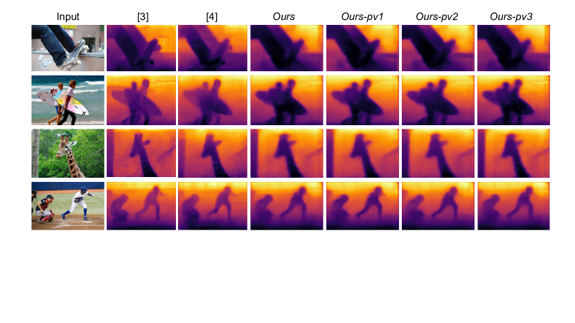
Figure 3: Zero-shot qualitative results on COCO dataset. From left to right; input, [3] (trained on NYUv2+DIW), [4] (trained on RedWeb+DIW+Y3D), ours, ours-prunedv1, ours-prunedv2 and ours-prunedv3. Ours are trained on DIW with knowledge distillation.

We compare our model against state-of-the-art methods on DIW. We exclusively report WHDR scores as it is the primary evaluation metric for depth in-the-wild scenarios, as explained in Section 3.2.1. Ours is our best model (i.e. last row of Table 6). Results are shown in Table 7.

Results show our approach has the best WHDR value where DIW is the only supervisory dataset. Models exceeding our results train on multiple datasets, which makes our model the most data efficient. Moreover, we train on a resolution of 224x448, whereas others train on larger resolutions ([4, 29, 46, 34] train on 384x384). A strong contender is [34], where a lightweight model trained on 256x256 resolution achieves 0.1344 WHDR. This is an impressive result despite not being trained on DIW, however this model is trained on ten other datasets and ours is better by 0.2 WHDR despite being smaller. All the successful methods use ResNet [11] architecture; our method outperforms them in cases where DIW is the only supervisory dataset, with a significantly less complex model. We also report the results of the pruned versions of our model (last three rows of Table 7). Our pruned model is still the best where DIW is the only supervisory dataset, with only 1M parameters.

Qualitative results are shown in Figure 3. Compared to larger models trained on multiple datasets including metric depth annotations, our results are competitive despite being trained only on ordinal pairs. Runtime results are shown in Table 8. [3] performs bad, especially on CPU, due to its non-mobile friendly architecture. [34] performs well, but can not achieve real-time on CPU. Compared with two other lightweight models, our model is significantly faster and reaches real-time on CPU and GPU with better WHDR.

Metric depth performance. We also report metric depth results despite training only on ordinal pairs. Two methods in Table 7 report metric results on NYU with models trained only on ordinal pairs and none report SI-RMSE on MC. [3] trains on NYU+DIW and [46] trains on NYU and report 1.10 and 1.07 RMSE on NYU, respectively. Ours achieves 1.30 RMSE (last row of Table 6), which is worse than the others. However, [46] trains on NYU and thus ”specialize” in indoor scenarios, and [3] trains on significantly more data. Improved performance on metric depth using only relative annotations is a future venue we are planning to explore, but is not within the scope of this study.

Method	Training Data	WHDR $\downarrow$	Parameter Count
Chen et al. [3]	DIW	0.2214	5.3M
Chen et al. [3]	NYU + DIW	0.1439	5.3M
Li [22]	MegaDepth	0.2297	5.3M
Xian et al. [46]	DIW	0.1498	53.1M
Xian et al. [46]	RW + DIW	0.1137	53.1M
Ranftl et al. [34]	RW + DL + MV + MD + WS	0.1246	105.3M
Ranftl et al. [34]	RW + DL + MV + MD + WS $\dagger$	0.1344	21.3M
Mertan et al. [29]	DIW	0.1250	53.1M
Mertan et al. [29]	RW + DIW	0.1101	53.1M
Chen et al. [4]	RW + DIW + Y3D	0.1059	53.1M
Our baseline	MC-RW-DIW	0.1316	2.6M
Ours	DIW (+ KD)	0.1156	2.6M
Ours-pruned v1	DIW (+ KD)	0.1190	1.9M
Ours-pruned v2	DIW (+ KD)	0.1196	1.5M
Ours-pruned v3	DIW (+ KD)	0.1208	1M

Table 7: Comparison with the state-of-the-art baselines on DIW test set. Several methods use the same architecture, therefore parameter counts for methods with no released weights are assumed to be the same. Row denoted with $\dagger$ trains on 10 datasets.

Device	Model	CPU	GPU	NNAPI
Samsung Galaxy S10+	[34]	274	99	332
	[3]	3361	390	1790
	Ours	116	74	108
	Ours -pruned v1	113	72	105
	Ours -pruned v2	104	69	103
	Ours -pruned v3	101	67	101
Samsung Galaxy S21	[34]	215	53	141
	[3]	3101	215	375
	Ours	54	27	43
	Ours -pruned v1	47	26	25
	Ours -pruned v2	43	25	35
	Ours -pruned v3	39	23	33

Table 8: Average runtime performances of our model and other lightweight methods [34, 3]. Runtime values are in ms and measured with same input resolution (256x256).

5 Conclusion

Monocular relative depth estimation is an important task in various applications, specifically in mobile settings. Therefore, it is imperative to design a model that is efficient and accurate in in-the-wild scenarios. To this end, we explore the design space of a lightweight relative depth estimator for mobile devices. Following a carefully performed model design process, we present a pipeline where we improve our model with a combination of knowledge distillation, intermediate predictions and loss rebalancing.

Our model achieves real-time performance on both mobile CPU and GPU and reaches 0.1156 WHDR on DIW, the best result among models that use only DIW as the supervisory dataset, with a fraction of model complexity. Our model, trained only on relative depth annotations, without pruning or hardware optimizations, has 2.6M parameters and runs with 37 FPS on a mobile GPU. A significantly pruned version achieves 0.1208 WHDR on DIW with 1M parameters and runs with 44 FPS on a mobile GPU.

References

- [1] Martín Abadi, Paul Barham, Jianmin Chen, Zhifeng Chen, Andy Davis, Jeffrey Dean, Matthieu Devin, Sanjay Ghemawat, Geoffrey Irving, Michael Isard, et al. Tensorflow: A system for large-scale machine learning. In 12th USENIX symposium on operating systems design and implementation (OSDI 16), pages 265–283, 2016.
- [2] Filippo Aleotti, Giulio Zaccaroni, Luca Bartolomei, Matteo Poggi, Fabio Tosi, and Stefano Mattoccia. Real-time single image depth perception in the wild with handheld devices. Sensors, 21(1):15, 2021.
- [3] Weifeng Chen, Zhao Fu, Dawei Yang, and Jia Deng. Single-image depth perception in the wild. In NIPS, pages 730–738, 2016.
- [4] Weifeng Chen, Shengyi Qian, and Jia Deng. Learning single-image depth from videos using quality assessment networks. In Proceedings of the IEEE/CVF Conference on Computer Vision and Pattern Recognition, pages 5604–5613, 2019.
- [5] David Eigen and Rob Fergus. Predicting depth, surface normals and semantic labels with a common multi-scale convolutional architecture. In Proceedings of the IEEE international conference on computer vision, pages 2650–2658, 2015.
- [6] David Eigen, Christian Puhrsch, and Rob Fergus. Depth map prediction from a single image using a multi-scale deep network. Advances in Neural Information Processing Systems, 27:2366–2374, 2014.
- [7] Ravi Garg, Vijay Kumar Bg, Gustavo Carneiro, and Ian Reid. Unsupervised cnn for single view depth estimation: Geometry to the rescue. In European conference on computer vision, pages 740–756. Springer, 2016.
- [8] Clément Godard, Oisin Mac Aodha, Michael Firman, and Gabriel J Brostow. Digging into self-supervised monocular depth estimation. In Proceedings of the IEEE/CVF International Conference on Computer Vision, pages 3828–3838, 2019.
- [9] Kai Han, Yunhe Wang, Qi Tian, Jianyuan Guo, Chunjing Xu, and Chang Xu. Ghostnet: More features from cheap operations. In Proceedings of the IEEE/CVF Conference on Computer Vision and Pattern Recognition, pages 1580–1589, 2020.
- [10] Kaiming He, Xiangyu Zhang, Shaoqing Ren, and Jian Sun. Delving deep into rectifiers: Surpassing human-level performance on imagenet classification. In Proceedings of the IEEE international conference on computer vision, pages 1026–1034, 2015.
- [11] Kaiming He, Xiangyu Zhang, Shaoqing Ren, and Jian Sun. Deep residual learning for image recognition. In Proceedings of the IEEE conference on computer vision and pattern recognition, pages 770–778, 2016.
- [12] Andrew Howard, Mark Sandler, Grace Chu, Liang-Chieh Chen, Bo Chen, Mingxing Tan, Weijun Wang, Yukun Zhu, Ruoming Pang, Vijay Vasudevan, et al. Searching for mobilenetv3. In Proceedings of the IEEE/CVF International Conference on Computer Vision, pages 1314–1324, 2019.
- [13] Junjie Hu, Mete Ozay, Yan Zhang, and Takayuki Okatani. Revisiting single image depth estimation: Toward higher resolution maps with accurate object boundaries. In 2019 IEEE Winter Conference on Applications of Computer Vision (WACV), pages 1043–1051. IEEE, 2019.
- [14] Adrian Johnston and Gustavo Carneiro. Self-supervised monocular trained depth estimation using self-attention and discrete disparity volume. In Proceedings of the IEEE/CVF Conference on Computer Vision and Pattern Recognition, pages 4756–4765, 2020.
- [15] Kevin Karsch, Ce Liu, and Sing Bing Kang. Depth transfer: Depth extraction from video using non-parametric sampling. IEEE transactions on pattern analysis and machine intelligence, 36(11):2144–2158, 2014.
- [16] Diederik P Kingma and Jimmy Ba. Adam: A method for stochastic optimization. In ICLR (Poster), 2015.
- [17] Janusz Konrad, Meng Wang, and Prakash Ishwar. 2d-to-3d image conversion by learning depth from examples. In 2012 IEEE Computer Society Conference on Computer Vision and Pattern Recognition Workshops, pages 16–22. IEEE, 2012.
- [18] Iro Laina, Christian Rupprecht, Vasileios Belagiannis, Federico Tombari, and Nassir Navab. Deeper depth prediction with fully convolutional residual networks. In 2016 Fourth international conference on 3D vision (3DV), pages 239–248. IEEE, 2016.
- [19] Jae-Han Lee, Minhyeok Heo, Kyung-Rae Kim, and Chang-Su Kim. Single-image depth estimation based on fourier domain analysis. In Proceedings of the IEEE Conference on Computer Vision and Pattern Recognition, pages 330–339, 2018.
- [20] Jae-Han Lee and Chang-Su Kim. Multi-loss rebalancing algorithm for monocular depth estimation. In Proceedings of the 2020 European Conference on Computer Vision (ECCV), Glasgow, UK, pages 23–28, 2020.
- [21] Zhengqi Li, Tali Dekel, Forrester Cole, Richard Tucker, Noah Snavely, Ce Liu, and William T Freeman. Learning the depths of moving people by watching frozen people. In Proceedings of the IEEE/CVF Conference on Computer Vision and Pattern Recognition, pages 4521–4530, 2019.
- [22] Zhengqi Li and Noah Snavely. Megadepth: Learning single-view depth prediction from internet photos. In Proceedings of the IEEE Conference on Computer Vision and Pattern Recognition, pages 2041–2050, 2018.
- [23] Beyang Liu, Stephen Gould, and Daphne Koller. Single image depth estimation from predicted semantic labels. In 2010 IEEE Computer Society Conference on Computer Vision and Pattern Recognition, pages 1253–1260. IEEE, 2010.
- [24] Fayao Liu, Chunhua Shen, and Guosheng Lin. Deep convolutional neural fields for depth estimation from a single image. In Proceedings of the IEEE conference on computer vision and pattern recognition, pages 5162–5170, 2015.
- [25] Miaomiao Liu, Mathieu Salzmann, and Xuming He. Discrete-continuous depth estimation from a single image. In Proceedings of the IEEE Conference on Computer Vision and Pattern Recognition, pages 716–723, 2014.
- [26] Yifan Liu, Changyong Shu, Jingdong Wang, and Chunhua Shen. Structured knowledge distillation for dense prediction. IEEE Transactions on Pattern Analysis and Machine Intelligence, 2020.
- [27] Ningning Ma, Xiangyu Zhang, Hai-Tao Zheng, and Jian Sun. Shufflenet v2: Practical guidelines for efficient cnn architecture design. In Proceedings of the European conference on computer vision (ECCV), pages 116–131, 2018.
- [28] Itzik Malkiel and Lior Wolf. Mtadam: Automatic balancing of multiple training loss terms. arXiv preprint arXiv:2006.14683, 2020.
- [29] Alican Mertan, Yusuf Huseyin Sahin, Damien Jade Duff, and Gozde Unal. A new distributional ranking loss with uncertainty: Illustrated in relative depth estimation. arXiv preprint arXiv:2010.07091, 2020.
- [30] Pushmeet Kohli Nathan Silberman, Derek Hoiem and Rob Fergus. Indoor segmentation and support inference from rgbd images. In ECCV, 2012.
- [31] Adam Paszke, Sam Gross, Francisco Massa, Adam Lerer, James Bradbury, Gregory Chanan, Trevor Killeen, Zeming Lin, Natalia Gimelshein, Luca Antiga, et al. Pytorch: An imperative style, high-performance deep learning library. Advances in Neural Information Processing Systems, 32:8026–8037, 2019.
- [32] Matteo Poggi, Filippo Aleotti, Fabio Tosi, and Stefano Mattoccia. Towards real-time unsupervised monocular depth estimation on cpu. In 2018 IEEE/RSJ International Conference on Intelligent Robots and Systems (IROS), pages 5848–5854. IEEE, 2018.
- [33] Matteo Poggi, Filippo Aleotti, Fabio Tosi, and Stefano Mattoccia. On the uncertainty of self-supervised monocular depth estimation. In Proceedings of the IEEE/CVF Conference on Computer Vision and Pattern Recognition, pages 3227–3237, 2020.
- [34] Rene Ranftl, Katrin Lasinger, David Hafner, Konrad Schindler, and Vladlen Koltun. Towards robust monocular depth estimation: Mixing datasets for zero-shot cross-dataset transfer. IEEE Transactions on Pattern Analysis and Machine Intelligence, 2020.
- [35] Olaf Ronneberger, Philipp Fischer, and Thomas Brox. U-net: Convolutional networks for biomedical image segmentation. In International Conference on Medical image computing and computer-assisted intervention, pages 234–241. Springer, 2015.
- [36] Mark Sandler, Andrew Howard, Menglong Zhu, Andrey Zhmoginov, and Liang-Chieh Chen. Mobilenetv2: Inverted residuals and linear bottlenecks. In Proceedings of the IEEE conference on computer vision and pattern recognition, pages 4510–4520, 2018.
- [37] Ashutosh Saxena, Min Sun, and Andrew Y Ng. Make3d: Learning 3d scene structure from a single still image. IEEE transactions on pattern analysis and machine intelligence, 31(5):824–840, 2008.
- [38] Evan Shelhamer, Jonathan T Barron, and Trevor Darrell. Scene intrinsics and depth from a single image. In Proceedings of the IEEE International Conference on Computer Vision Workshops, pages 37–44, 2015.
- [39] Mingxing Tan, Bo Chen, Ruoming Pang, Vijay Vasudevan, Mark Sandler, Andrew Howard, and Quoc V Le. Mnasnet: Platform-aware neural architecture search for mobile. In Proceedings of the IEEE/CVF Conference on Computer Vision and Pattern Recognition, pages 2820–2828, 2019.
- [40] Mingxing Tan and Quoc Le. Efficientnet: Rethinking model scaling for convolutional neural networks. In International Conference on Machine Learning, pages 6105–6114. PMLR, 2019.
- [41] Mingxing Tan and Quoc V Le. Mixconv: Mixed depthwise convolutional kernels. arXiv preprint arXiv:1907.09595, 2019.
- [42] Xiaohan Tu, Cheng Xu, Siping Liu, Renfa Li, Guoqi Xie, Jing Huang, and Laurence Tianruo Yang. Efficient monocular depth estimation for edge devices in internet of things. IEEE Transactions on Industrial Informatics, 2020.
- [43] Lijun Wang, Jianming Zhang, Oliver Wang, Zhe Lin, and Huchuan Lu. Sdc-depth: Semantic divide-and-conquer network for monocular depth estimation. In Proceedings of the IEEE/CVF Conference on Computer Vision and Pattern Recognition, pages 541–550, 2020.
- [44] Diana Wofk, Fangchang Ma, Tien-Ju Yang, Sertac Karaman, and Vivienne Sze. Fastdepth: Fast monocular depth estimation on embedded systems. In 2019 International Conference on Robotics and Automation (ICRA), pages 6101–6108. IEEE, 2019.
- [45] Bichen Wu, Xiaoliang Dai, Peizhao Zhang, Yanghan Wang, Fei Sun, Yiming Wu, Yuandong Tian, Peter Vajda, Yangqing Jia, and Kurt Keutzer. Fbnet: Hardware-aware efficient convnet design via differentiable neural architecture search. In Proceedings of the IEEE/CVF Conference on Computer Vision and Pattern Recognition, pages 10734–10742, 2019.
- [46] Ke Xian, Chunhua Shen, Zhiguo Cao, Hao Lu, Yang Xiao, Ruibo Li, and Zhenbo Luo. Monocular relative depth perception with web stereo data supervision. In Proceedings of the IEEE Conference on Computer Vision and Pattern Recognition, pages 311–320, 2018.
- [47] Ke Xian, Jianming Zhang, Oliver Wang, Long Mai, Zhe Lin, and Zhiguo Cao. Structure-guided ranking loss for single image depth prediction. In Proceedings of the IEEE/CVF Conference on Computer Vision and Pattern Recognition, pages 611–620, 2020.
- [48] Dan Xu, Wei Wang, Hao Tang, Hong Liu, Nicu Sebe, and Elisa Ricci. Structured attention guided convolutional neural fields for monocular depth estimation. In Proceedings of the IEEE conference on computer vision and pattern recognition, pages 3917–3925, 2018.
- [49] Tien-Ju Yang, Andrew Howard, Bo Chen, Xiao Zhang, Alec Go, Mark Sandler, Vivienne Sze, and Hartwig Adam. Netadapt: Platform-aware neural network adaptation for mobile applications. In Proceedings of the European Conference on Computer Vision (ECCV), pages 285–300, 2018.
- [50] Wei Yin, Yifan Liu, Chunhua Shen, and Youliang Yan. Enforcing geometric constraints of virtual normal for depth prediction. In Proceedings of the IEEE/CVF International Conference on Computer Vision, pages 5684–5693, 2019.
- [51] Linfeng Zhang, Jiebo Song, Anni Gao, Jingwei Chen, Chenglong Bao, and Kaisheng Ma. Be your own teacher: Improve the performance of convolutional neural networks via self distillation. In Proceedings of the IEEE/CVF International Conference on Computer Vision, pages 3713–3722, 2019.