Supplementary Material

1 Periodgrams or space-time plots for all temperature gradients

Here, we present the periodgrams at different temperature gradients only for a selected duration of time. The actual time sequences are 26 times longer than presented in each of these periodgrams. In general, we observe that the waves become weaker with increasing temperature gradient as the microparticle cloud moves away from the sheath region and into the bulk region.
At some temperature gradients in the images shown below, for example at $\Delta T=10K$, we see no wavecrests in the chosen time window. However at a higher temperature gradient, for example at $\Delta T=12.5K$, we see the wave crests again. Here, we would like to stress that this is not due to any physical reasons. It is simply because the time sequence shown here does not include any wave crests at $\Delta T=10K$. However, if we look at a later time sequence instance at $\Delta T=10K$, as shown in Fig. 16, we can see wave crests at this temperature gradient as well. We must remember that these waves become very weak at higher temperature differences as the dust cloud moves away from the sheath region.

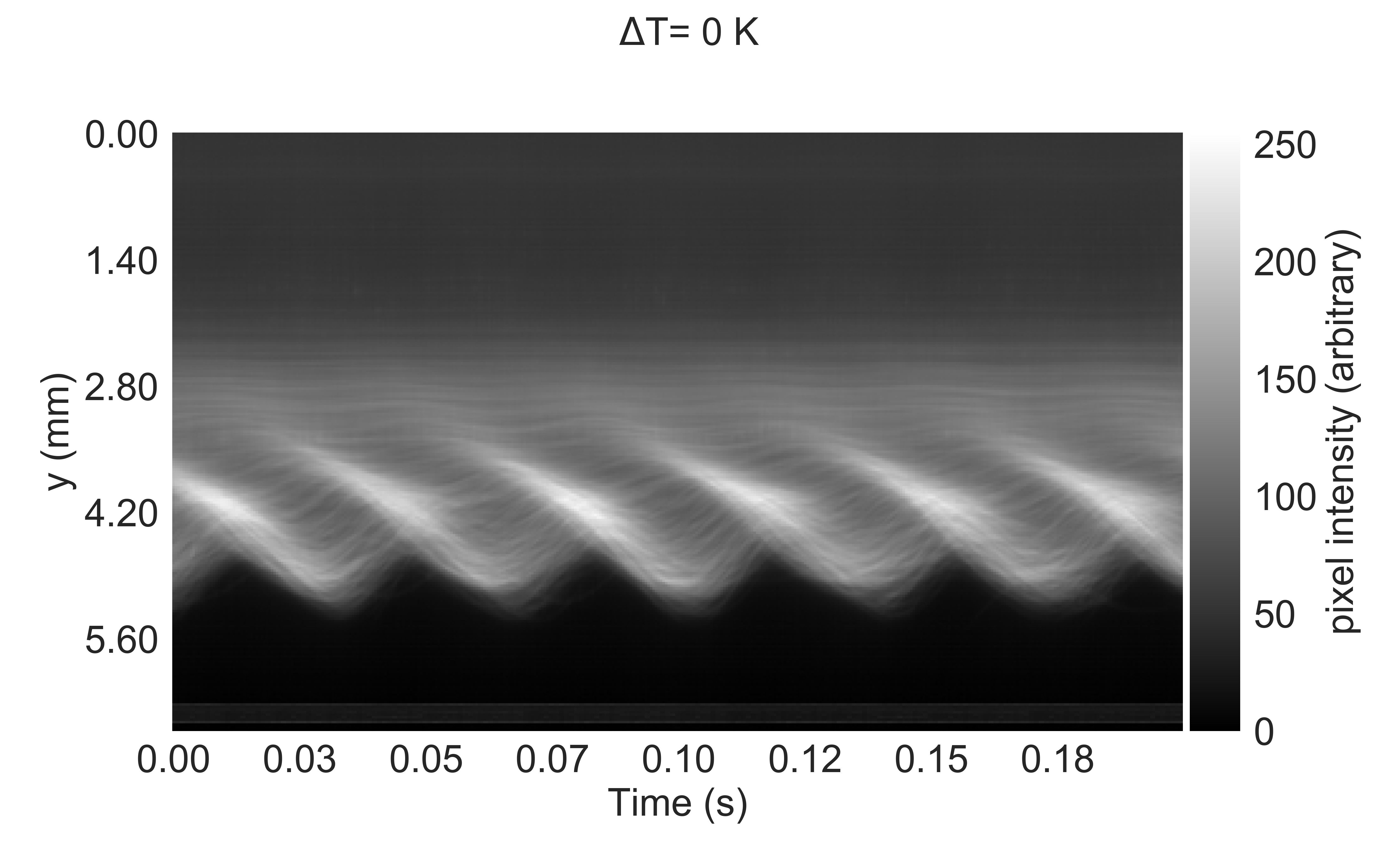
Figure 1: Periodgram or space-time plot at $\Delta T=0K$ showing only a small time sequence instance.

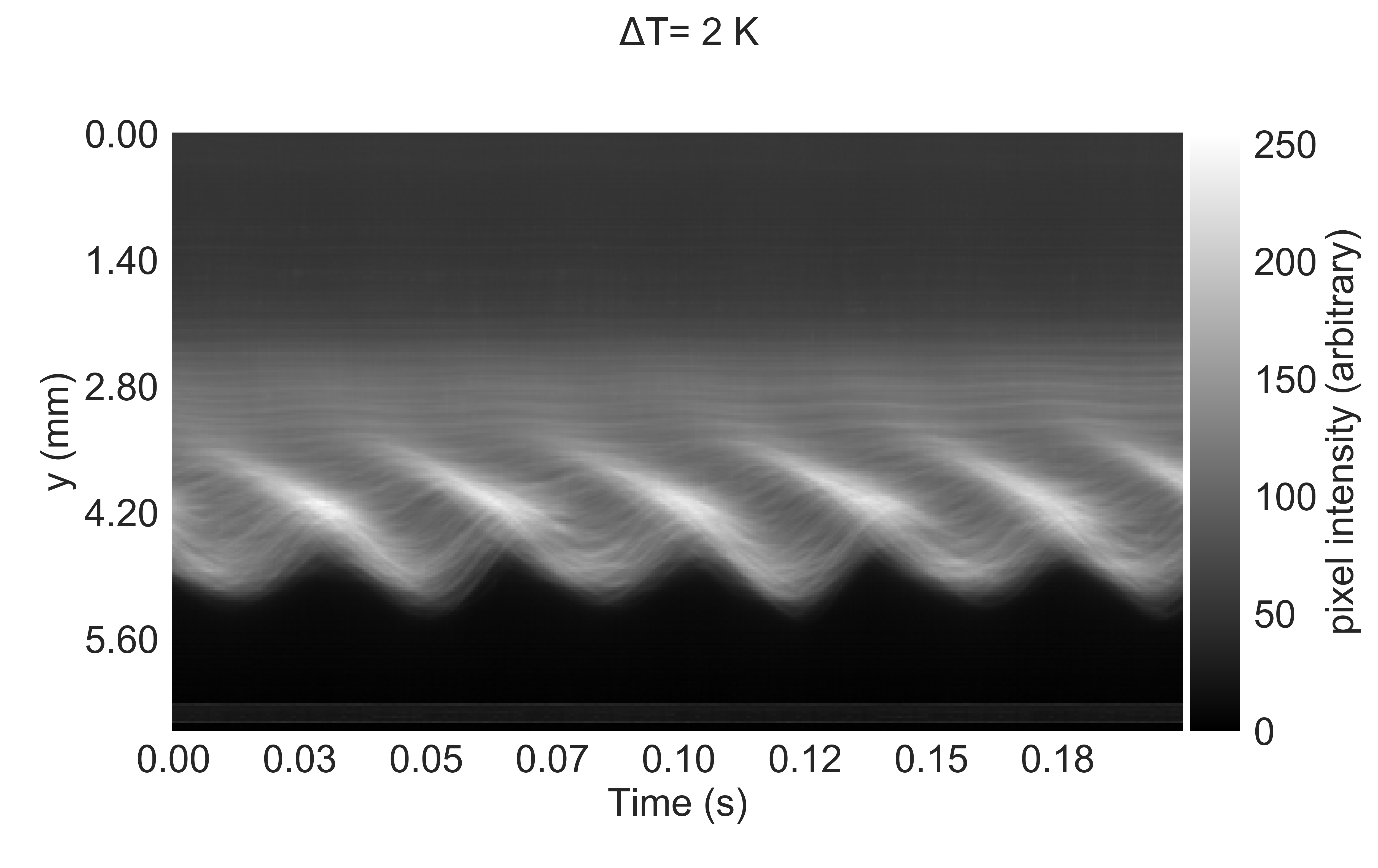
Figure 2: Periodgram or space-time plot at $\Delta T=2K$ showing only a small time sequence instance.

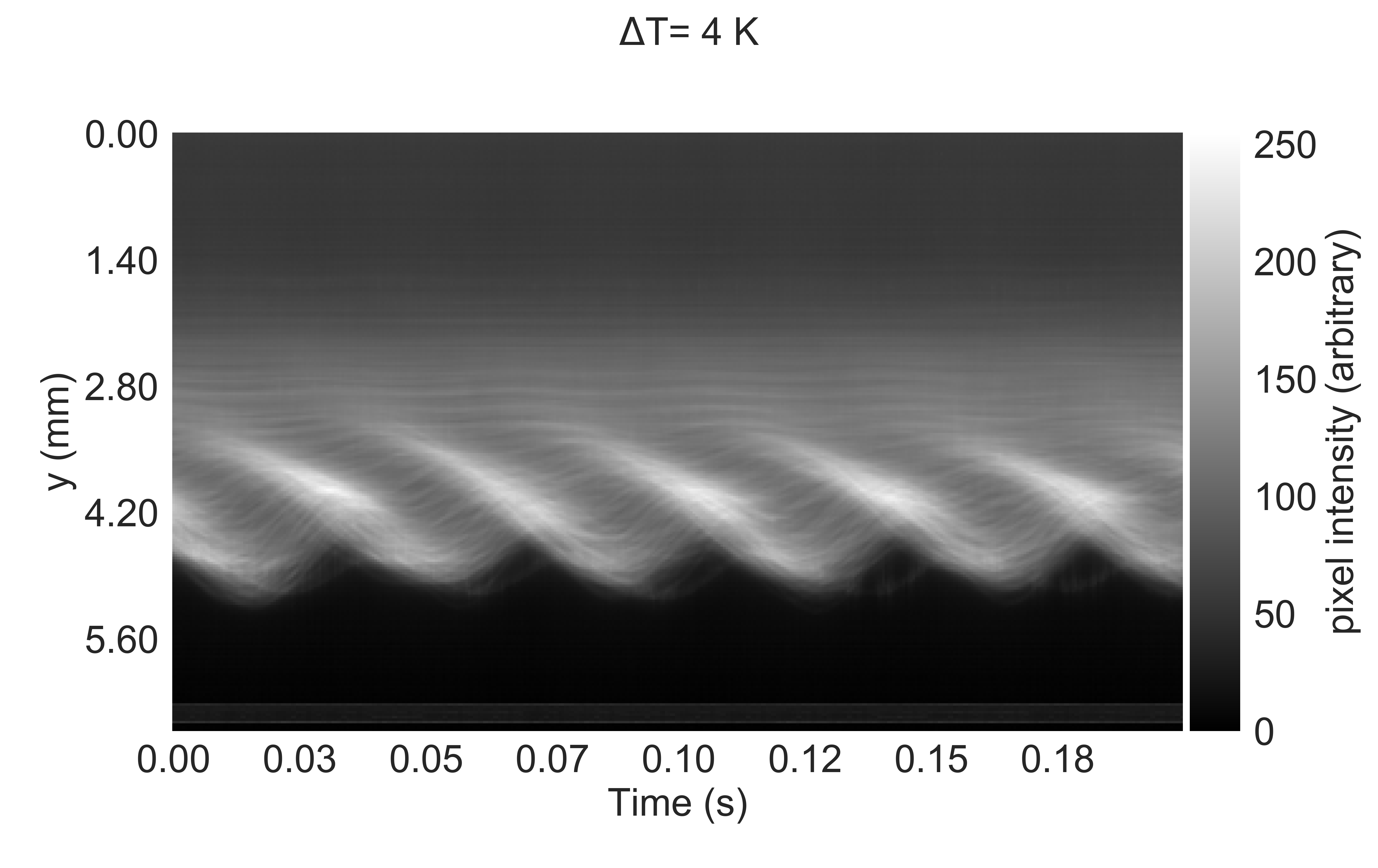
Figure 3: Periodgram or space-time plot at $\Delta T=4K$ showing only a small time sequence instance.

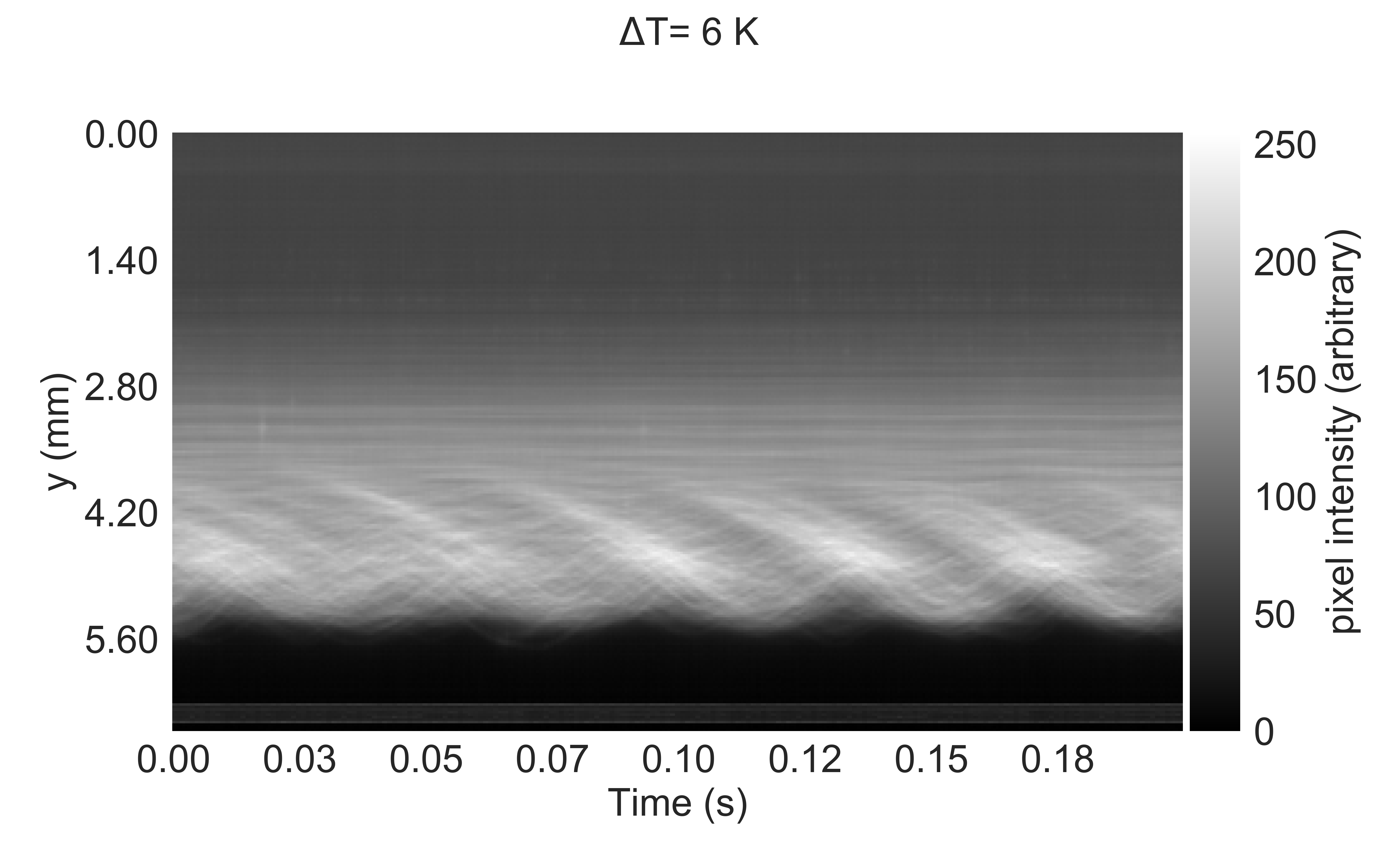
Figure 4: Periodgram or space-time plot at $\Delta T=6K$ showing only a small time sequence instance.

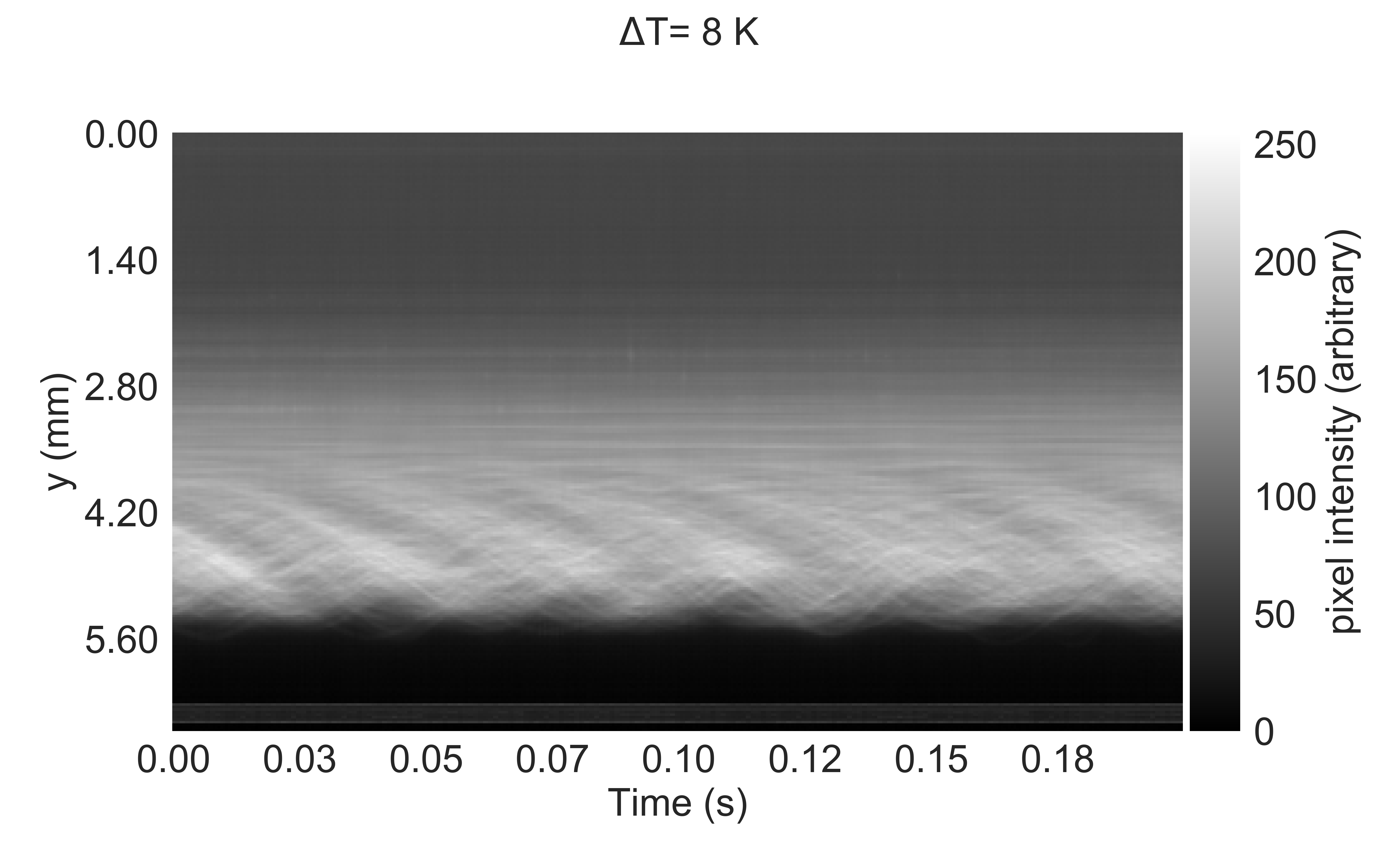
Figure 5: Periodgram or space-time plot at $\Delta T=8K$ showing only a small time sequence instance.

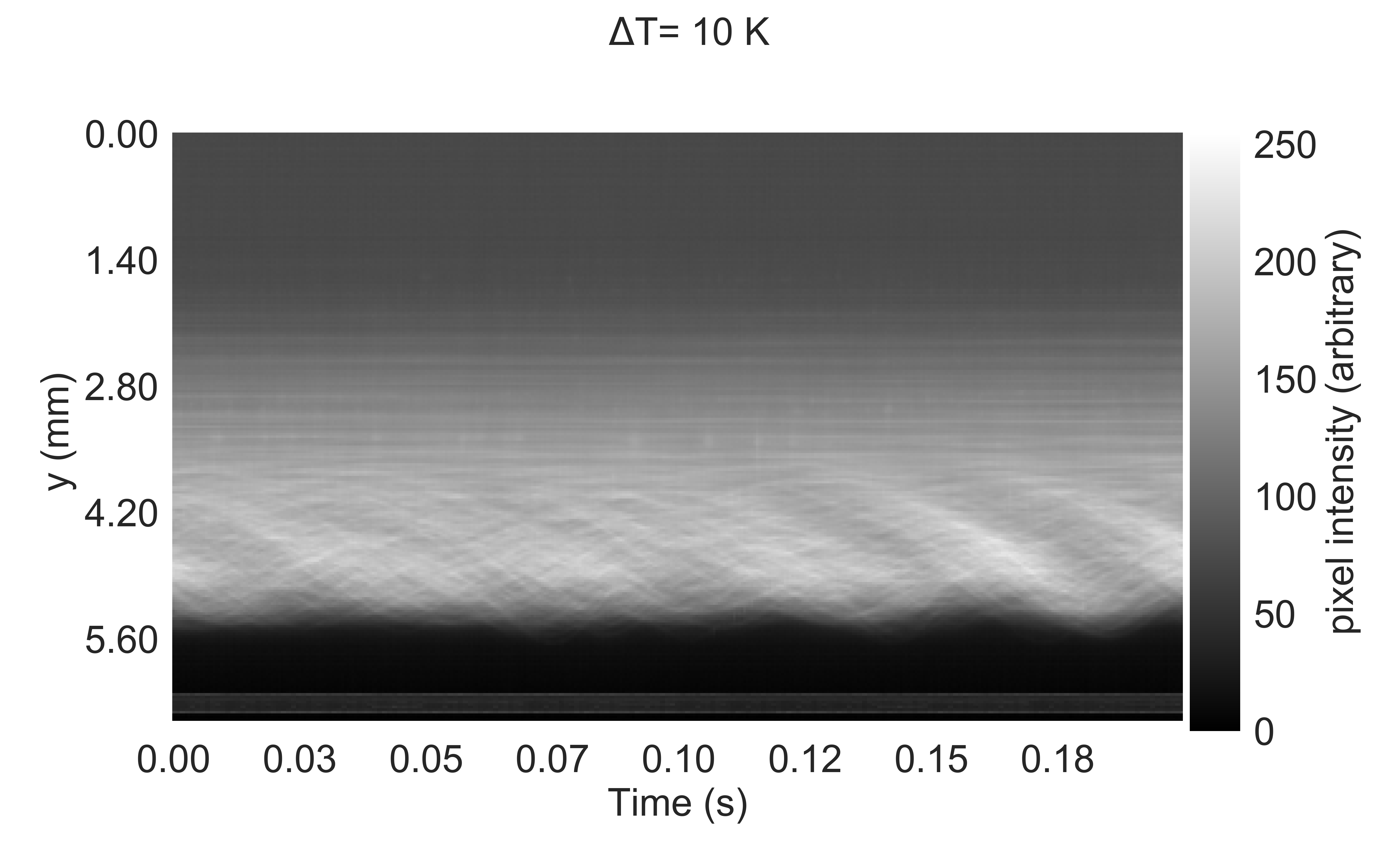
Figure 6: Periodgram or space-time plot at $\Delta T=10K$ showing only a small time sequence instance.

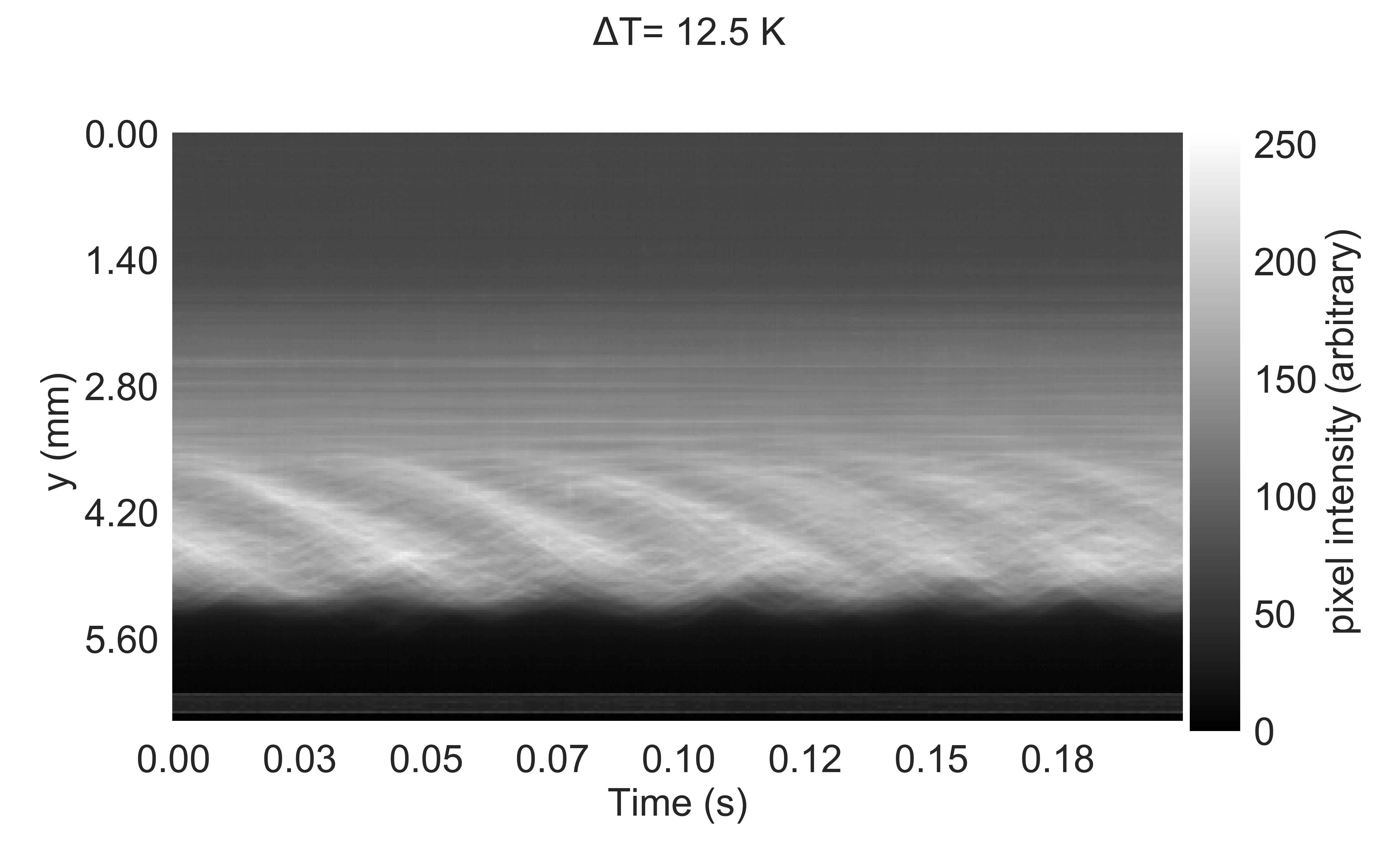
Figure 7: Periodgram or space-time plot at $\Delta T=12.5K$ showing only a small time sequence instance.

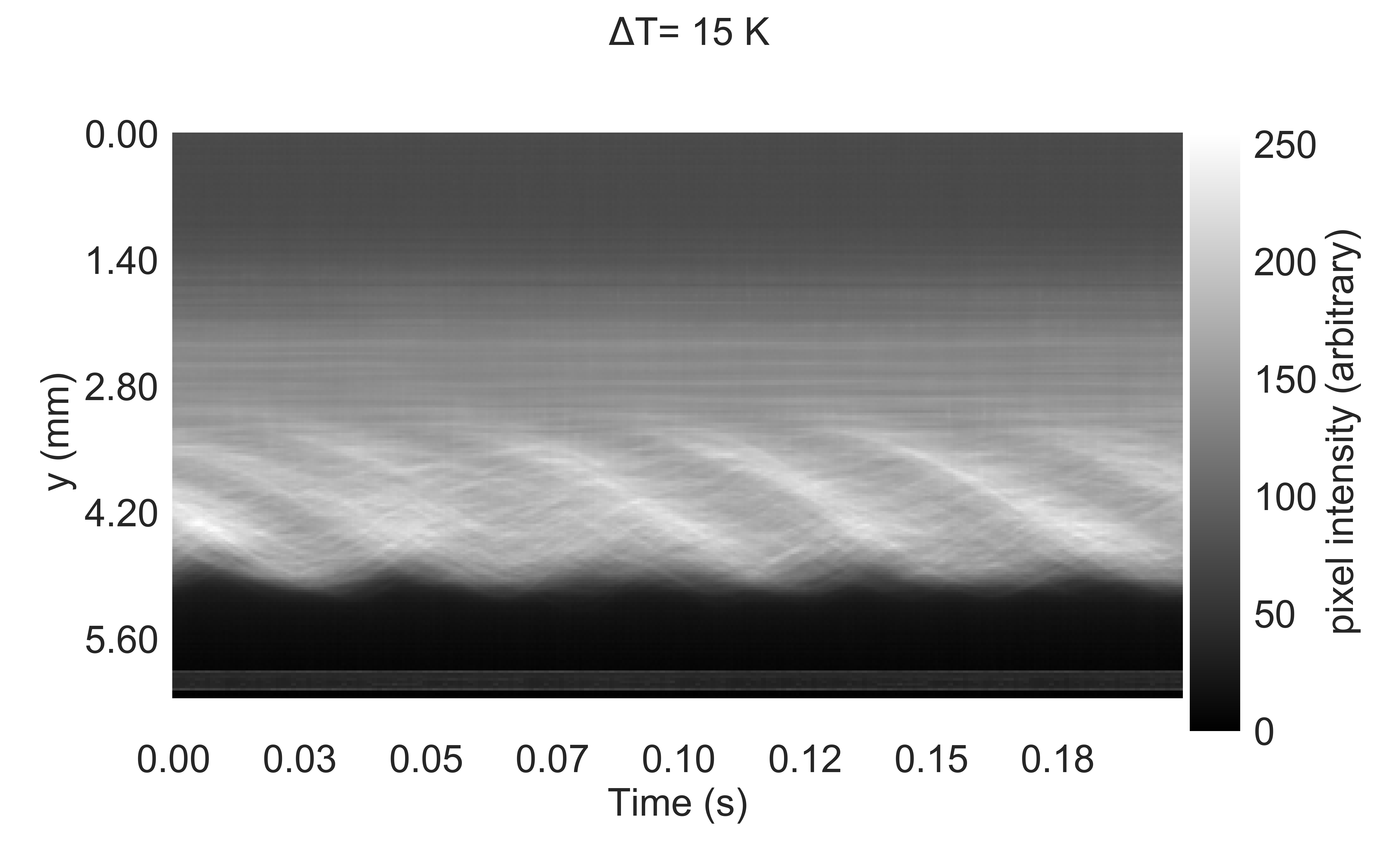
Figure 8: Periodgram or space-time plot at $\Delta T=15K$ showing only a small time sequence instance.

Figure 9: Periodgram or space-time plot at $\Delta T=17.5K$ showing only a small time sequence instance.

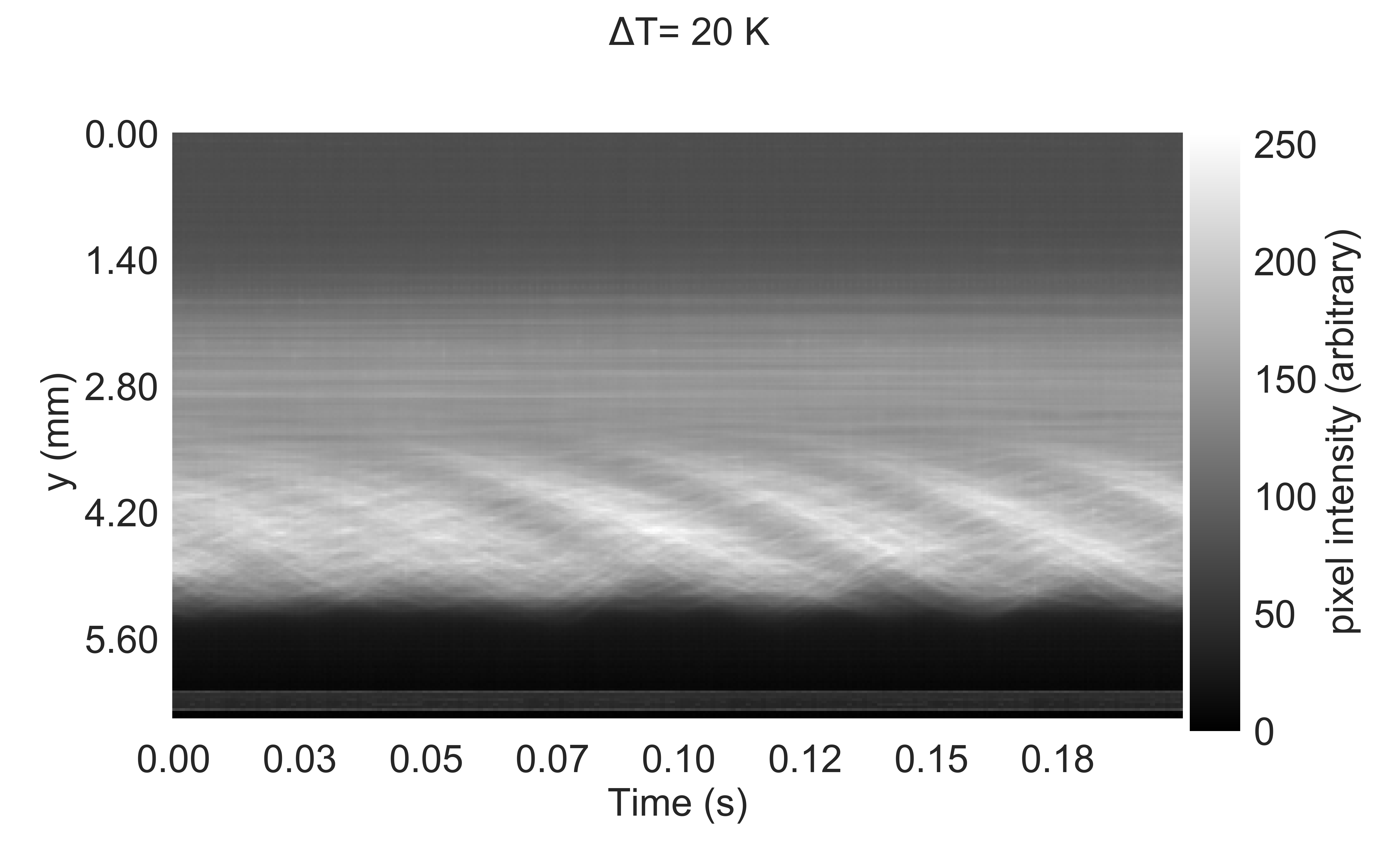
Figure 10: Periodgram or space-time plot at $\Delta T=20K$ showing only a small time sequence instance.

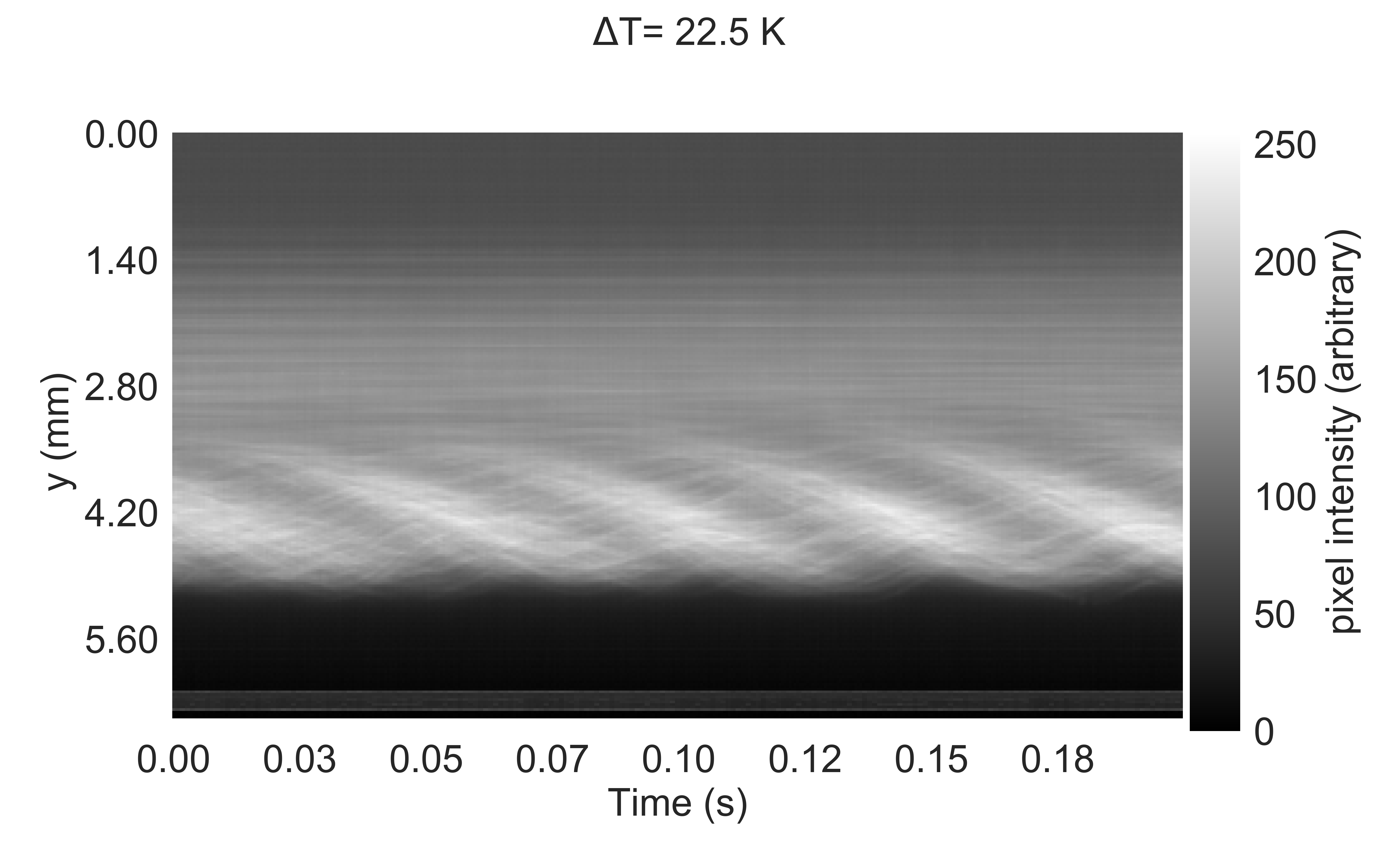
Figure 11: Periodgram or space-time plot at $\Delta T=22.5K$ showing only a small time sequence instance.

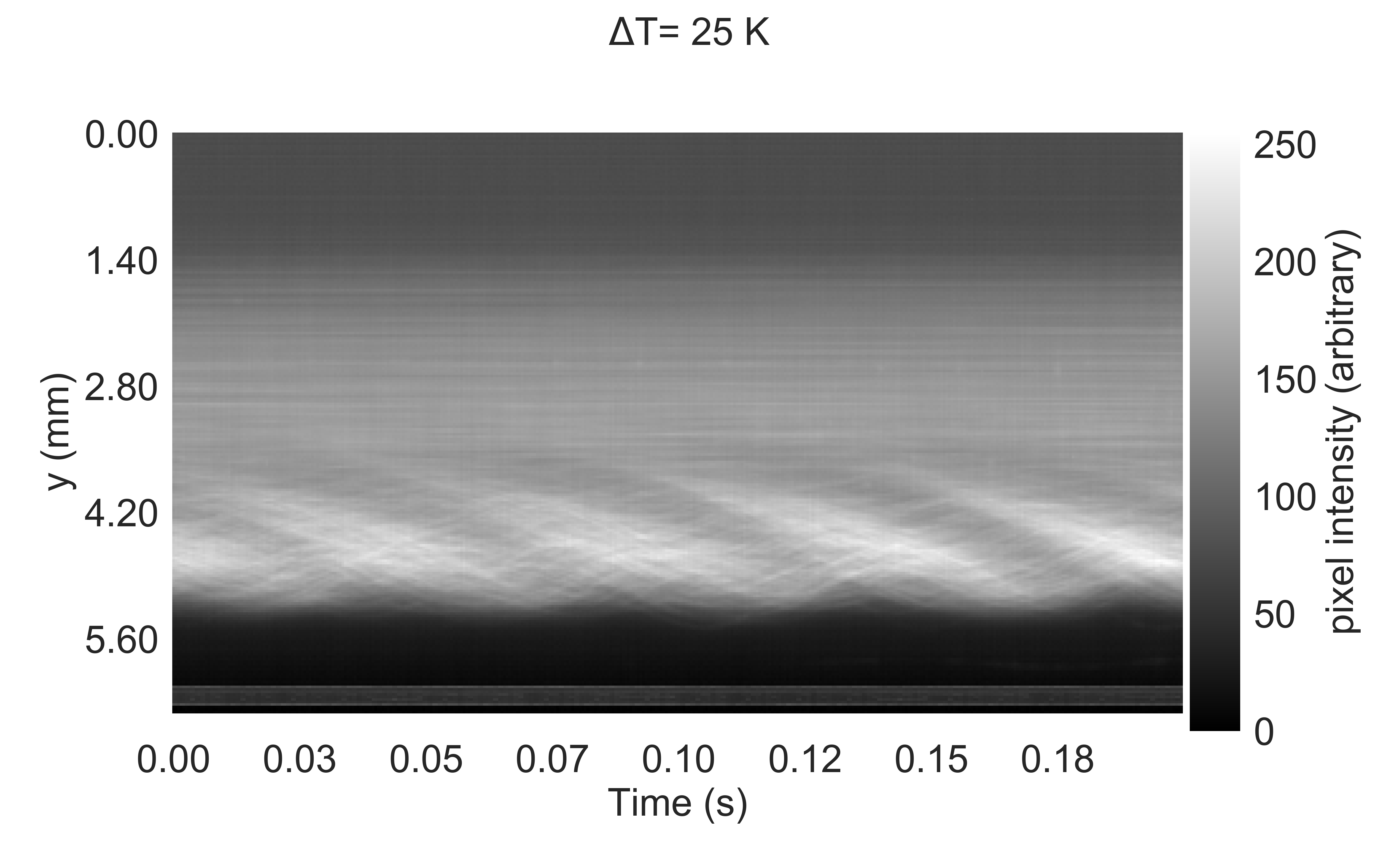
Figure 12: Periodgram or space-time plot at $\Delta T=25K$ showing only a small time sequence instance.

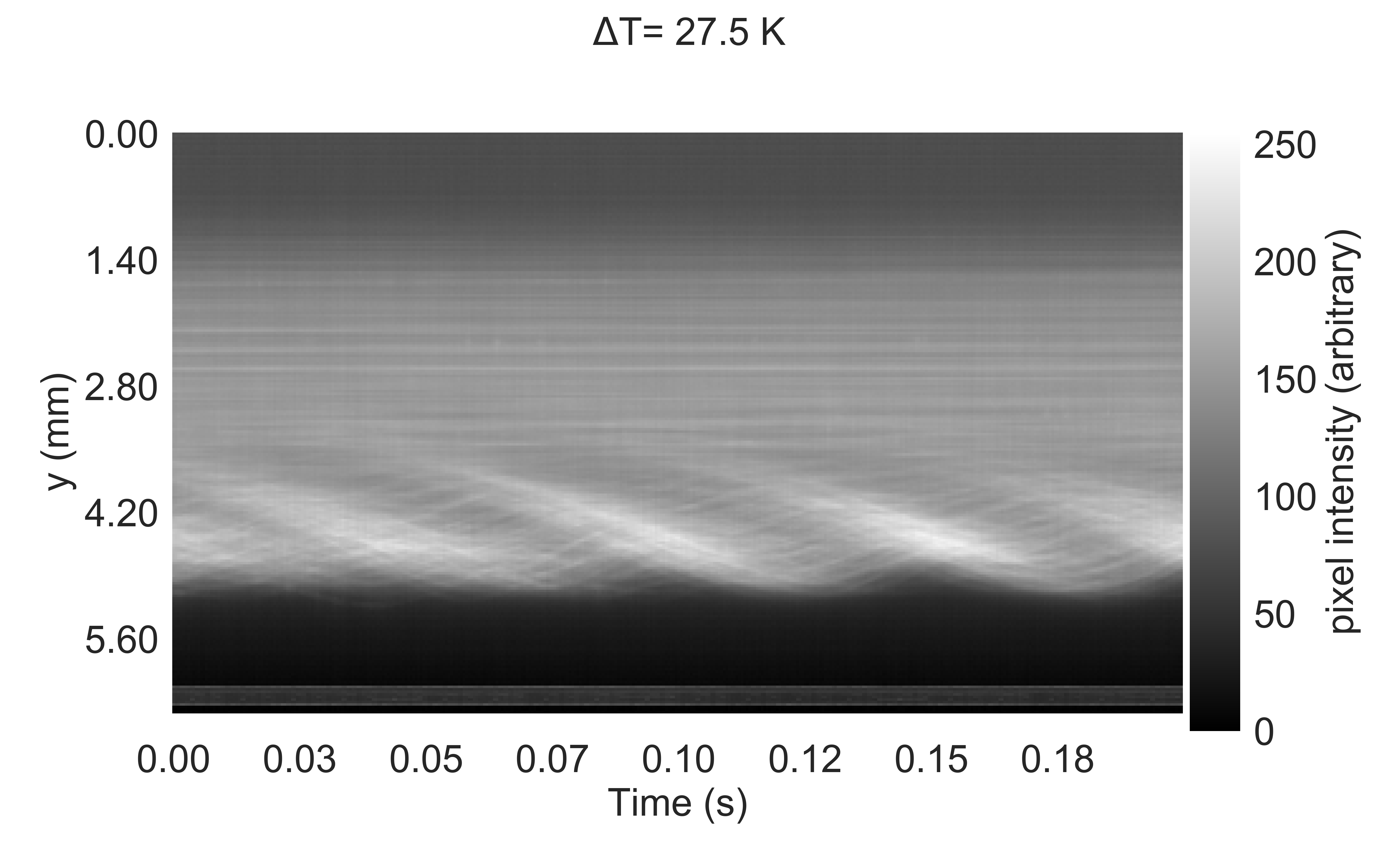
Figure 13: Periodgram or space-time plot at $\Delta T=27.5K$ showing only a small time sequence instance.

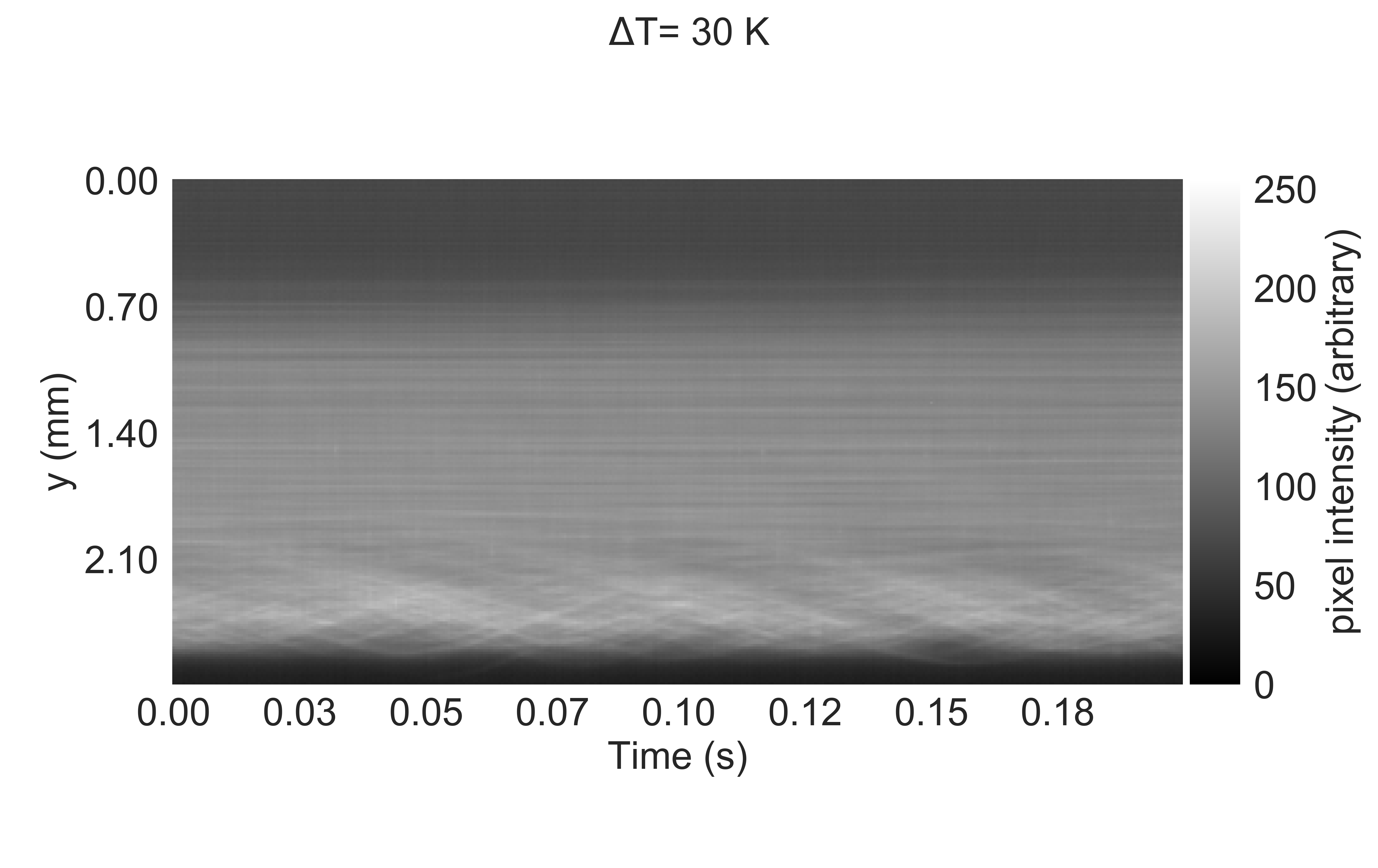
Figure 14: Periodgram or space-time plot at $\Delta T=30K$ showing only a small time sequence instance.

Figure 15: Periodgram or space-time plot at $\Delta T=22.5K$ showing only a small time sequence instance.

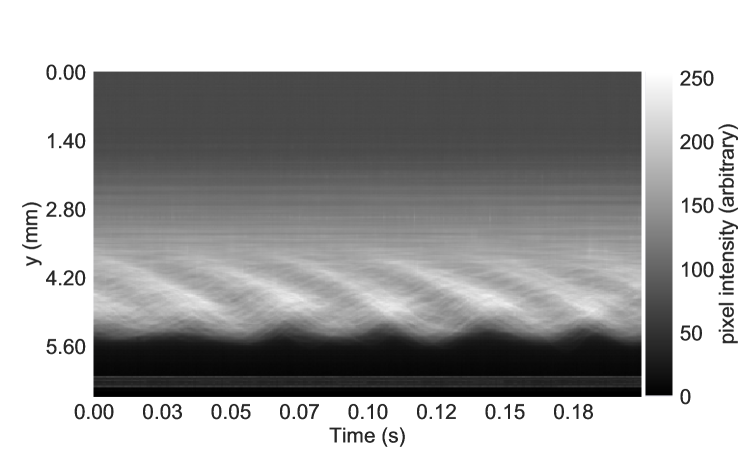
Figure 16: Periodgram or space-time plot at $\Delta T=10K$ showing only a small time sequence instance, which is different from the time sequence instance shown in Fig. 6.

2 Measuring wave frequency using template matching

As mentioned in the manuscript in Section IIB and shown here in Fig. 17, the results for frequency calculations using template matching gives very high standard deviation. The reason for this is that the wave crest is not always clear, for instance at $\Delta T=10K$ in Fig. 6, where we observe only 2 wave crests in the selected time region. In such cases, the template matching method is not able to find two consecutive crests, which leads to very high error in calculation of average DDW frequency.

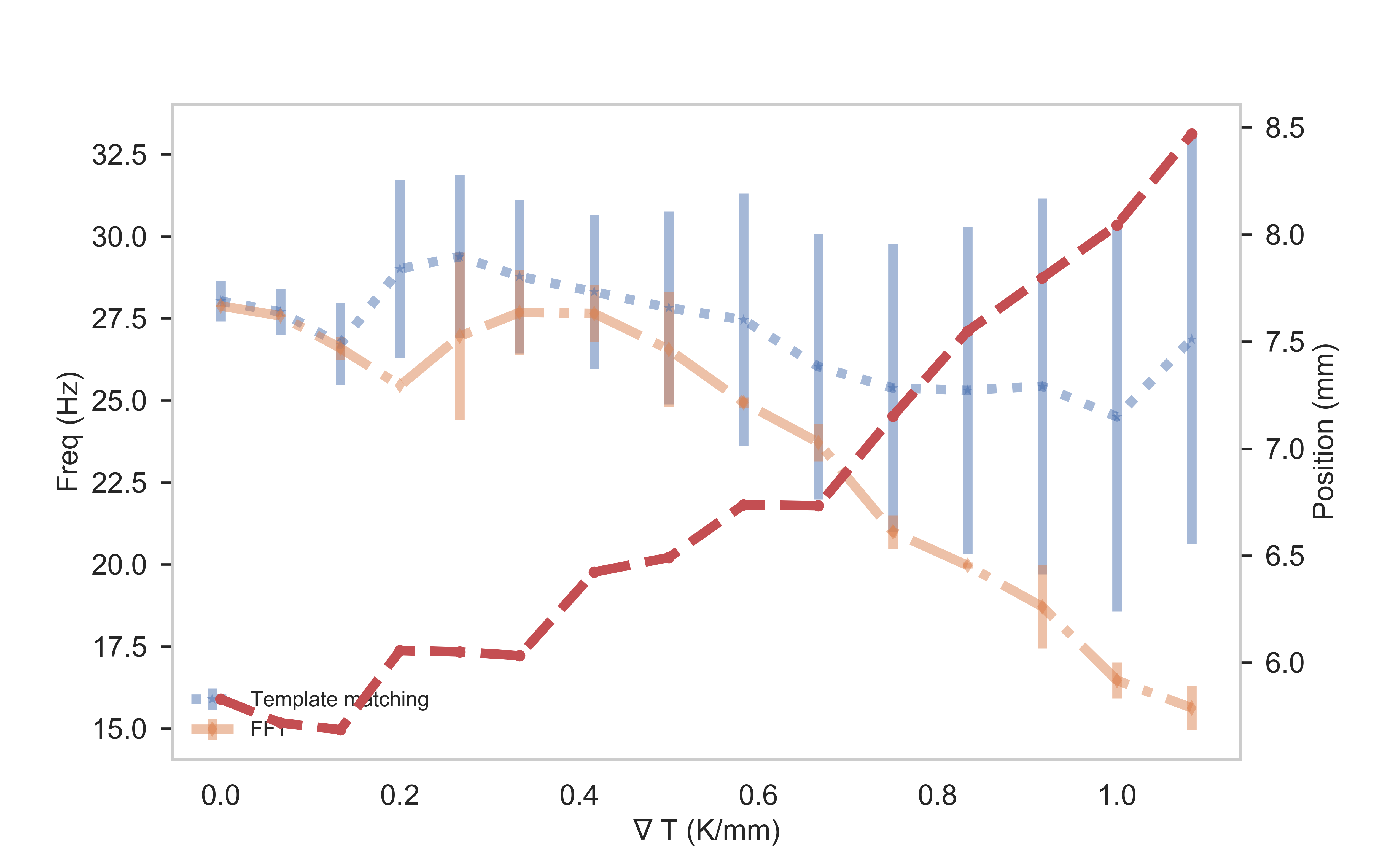
Figure 17: Average wave frequency versus temperature gradient. The line in blue shows the frequency found using the method of template matching and the line in orange shows the frequency found by making a Fast Fourier Transform (FFT) of the change in average particle velocity with time (refer Fig. 5 in the manuscript). The vertical lines are the standard deviations. It is evident from this plot that the standard deviation is extremely high for the template matching method, especially at high temperature gradients. This is the reason we choose to report our results only using the method of fourier transform of tracked particle velocities in time.

3 Calculation of practical fit for particle number density v/s temperature gradient

Figure 18: Variation of particle number density with temperature difference calculated using raw images from the experiment.

The calculation of the change in dust number density with temperature gradient was done using experimental images by calculating the pair correlation function of located particles in the raw image at each temperature difference selected for the experiment. Fig. 18 shows the change in particle number density with temperature difference, calculated using experimental images. After performing a fit on this data, the following correlation was found between the particle number density and temperature gradient: $n_{p}\approx 8\times 10^{4}-3\times 10^{3}\,\nabla T$, where $n_{p}$ is expressed in cm^-3 and $\nabla$T is expressed in K/cm. Hence, this can be used as a practical fit for the very basic theoretical estimates performed in the paper in Section IIIB.