Hyperparameter Selection for Imitation Learning

Abstract

We address the issue of tuning hyperparameters (HPs) for imitation learning algorithms in the context of continuous-control, when the underlying reward function of the demonstrating expert cannot be observed at any time. The vast literature in imitation learning mostly considers this reward function to be available for HP selection, but this is not a realistic setting. Indeed, would this reward function be available, it could then directly be used for policy training and imitation would not be necessary. To tackle this mostly ignored problem, we propose a number of possible proxies to the external reward. We evaluate them in an extensive empirical study (more than 10’000 agents across 9 environments) and make practical recommendations for selecting HPs. Our results show that while imitation learning algorithms are sensitive to HP choices, it is often possible to select good enough HPs through a proxy to the reward function.

1 Introduction

Recent advances in Reinforcement Learning (RL) now allow optimizing control policies with respect to a given reward function even for high-dimensional observation and action spaces (Berner et al., 2019; Vinyals et al., 2019). However, in many cases it is impossible or impractical to design a reward function which captures the desired outcomes (Popov et al., 2017). One of the approaches to overcome this issue is Imitation Learning (IL), which relies on a set of demonstrations presenting the desired behaviour instead of a reward signal (Schaal, 1999; Argall et al., 2009). IL can be achieved through pure supervised learning (Pomerleau, 1991) but many IL approaches leverage the assumption that the expert implements an optimal policy according to an unknown reward function. This approach, also known as Inverse Reinforcement Learning (IRL), tries to recover this unknown reward function and use an RL algorithm to train a policy to maximize it (Russell, 1998; Ng et al., 2000; Ziebart et al., 2008). Both approaches have their advantages and drawbacks (Piot et al., 2013).

While all machine learning approaches require some degree of hyperparameter (HP) tuning, the issue is especially pronounced in RL. Indeed, RL algorithms are known to be very sensitive to the values of their numerous HPs (Henderson et al., 2018; Andrychowicz et al., 2020). RL algorithms’ HPs are usually chosen by letting different agents interact with the environment and selecting the one which performed best as measured with the environment reward.

Surprisingly, this is also a common practice in the IL domain where one does not have access to an environment reward function which accurately describes the task. If such a reward were known, it could be directly used to train a controller via RL. Although expert trajectories can also be useful in this case, this is not the setting of IL, but of RL with demonstrations where both the expert demonstrations and reward signals are used (Kim et al., 2013; Piot et al., 2014; Hester et al., 2018). This constitutes a gap between the IL framework and the experimental design of IL agents that hinders the practical utility of IL. It is indeed unclear how to tune the imitation agent without access to the reward function.

In some cases, although a per-step reward function is not available, a success signal can be computed or given by a human rater. We focus on the tasks for which (1) such signal is not available or (2) the cost of such signal is prohibitive or (3) such signal could bias the resulting policy. Indeed, just as the reward-engineering problem leads to policies maximizing a reward in an unexpected way (Sims, 1994; Feldt, 1998; Ecoffet et al., 2021), selecting policies on the basis of an incautiously designed metric or of a biased human judgement can lead to biased policies (Henderson et al., 2018).

We present a thorough empirical study of this question in a number of challenging domains with high dimensional spaces of actions and observations. We train thousands of agents, using three IL algorithms based on different paradigms, with large parameter sweeps, and empirically compare different HP selection strategies. In particular, we consider a number of metrics assessing how well the learned behaviors match the demonstrations. Moreover, we investigate how well the algorithms perform if their HPs are selected on a similar task where the reward signal is assumed to be available. As our key contributions, we:

• highlight the fundamental question of HP selection in IL without access to an external reward signal;

• provide empirical evidence that the results obtained by IL algorithms depend heavily on how HPs are selected, confirming the prominence of the problem;

• propose proxy metrics to define the task success;

• perform a thorough comparison of these alternatives to the external reward signal in a large-scale study;

• empirically assess the transferability of HPs across tasks for different IL algorithms;

• give practical recommendations for tuning HPs in IL.

2 Hyperparameter Selection

In this paper, we argue that HP selection should strictly follow the setup in which the algorithm is to be used. For example, when designing an offline RL algorithm, HPs should not be tuned through environment interactions but rather offline (Paine et al., 2020). Similarly, in IL, one can interact with the environment but should choose HPs without access to the reward signal. We propose to choose these HPs by either (1) using proxy metrics or (2) transferring HPs from other environments that have an accessible reward.

2.1 Using proxy metrics

To select a model, one should use a different metric than the return under the supposedly unknown reward. We include a diverse set of metrics that can be used to measure the success of a policy in imitating the demonstrations.

Action MSE. The simplest way to measure similarity between agent behaviour and a given set of demonstrations is to compare actions of the agent and the demonstrator on the states provided in the demonstrations. In particular, for continuous control environments, we use the mean squared error (MSE) between the agent and the expert actions on the training expert states. Notice that this can be done offline without any interaction with the environment. For every environment, we also keep some expert trajectories as a validation set and use it to compute the validation MSE. This will allow us to study if selecting HPs on validation data helps avoiding overfitting, notably as action MSE is actually the loss optimized by the Behavioral Cloning (Pomerleau, 1991) algorithm.

State distribution divergence. Another approach to measuring how well the learned policy imitates the expert is by comparing the distributions of states encountered by both policies. In particular, we compute the Wasserstein distance (Villani, 2008) between the distribution of states in the demonstrations and that of the agent (i.e. from generated trajectories). As before, we measure both the distance to the training set and to the validation set and thus have two distinct metrics. The Wasserstein metric computation assumes we can compute distances in the state space, to this end we use the Euclidean distance with state coordinates normalized to have the standard deviation equal to $1$. While this is not directly applicable to vision-based observations, there are plenty of techniques which can be used to compute vector embedding for vision observations in RL/IL, e.g. Stooke et al. (2020); Lee et al. (2020).

Random Network Distillation (RND). As proposed by Burda et al. (2018); Wang et al. (2019), we define a support estimation metric by taking two randomly initialized networks, and train one to predict the random output of the other one on the expert training set. The metric is then given by the MSE between the prediction network and the frozen one on trajectories generated by the agent. Details on the metric training are given in Appx. A.4.

Imitation Return. IRL algorithms recover a –learned– reward function. We can use the corresponding learned return to select HPs. We compute this metric as it should model the goal optimized by the agent, although this goal is generally non-stationary. Moreover, the scale of the metric often depends on the HPs which could make it harder to compare the value of this metric between different training runs.

Environment return. This is the sum of rewards obtained during a full episode according to the environment reward function. We include it as the gold standard.

A desired property for all these metrics is to preserve the ranking of policies induced by the oracle environment return. A metric that would satisfy this property would yield an optimal HP selection. Note that this is a sufficient but not a necessary condition. We show in Appx B.1, using both the Spearman rank correlation and the ROC-AUC of an additional task (classify good from poor policies), that the aforementioned metrics have good enough ranking properties to make them legitimate candidates for HP selection.

2.2 Transfer scenario

The HPs that work best in tasks for which a well-defined reward function is available can also be transferred to a new task. We expect the success of this procedure to highly depend on the similarity between the source and target domains.

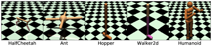
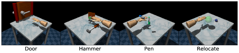
Figure 1: Environments: OpenAI Gym (top) and Adroit (bottom).

2.3 Environments and data

We focus on continuous-control benchmarks and consider five widely used environments from OpenAI Gym (Brockman et al., 2016): Hopper-v2, Walker2d-v2, HalfCheetah-v2, Ant-v2, and Humanoid-v2 and four manipulation tasks from Adroit (Kumar, 2016): pen-v0, relocate-v0, door-v0, and hammer-v0. The Adroit tasks respectively consist in aligning a pen with a target orientation, moving an object to a target location, opening a door and hammering a nail. These two benchmarks bring orthogonal contributions. The former focuses on locomotion but has 5 environments with different state/action dimensionality. The latter, more varied in term of tasks, has an almost constant state-action space. For the Gym tasks, we generate demonstrations with a Soft Actor-Critic (SAC) (Haarnoja et al., 2018a) agent trained on the environment reward. For the Adroit environments, we use the “expert” datasets from the D4RL dataset (Fu et al., 2020).

For the OpenAI Gym environments, we use 11 training trajectories and keep 5 additional held-out trajectories for validation. For the Adroit environments, 20 training trajectories are used as well as 5 validation trajectories. The number of training trajectories corresponds to what IL algorithms are typically designed for. We chose a low number of validation trajectories as demonstrations are generally expensive and one wishes to use as many as possible for training.

2.4 Algorithms

We consider the three algorithms briefly described below. They use different approaches, from supervised learning, to Inverse RL via distribution matching, either through the primal or the dual form of a divergence. We consider them to be representative of different families of algorithms and thus good candidates to validate HP selection techniques.

Detailed description of the algorithms can be found in the original publications. We provide additional information on our implementations in Appx. A. We implemented our algorithms in the Acme framework (Hoffman et al., 2020) using JAX (Bradbury et al., 2018) for automatic differentiation and Flax (Heek et al., 2020) for neural networks computation.

Behavioral Cloning (BC, Pomerleau (1991)) is the simplest approach to IL and relies on mapping the expert states to the expert actions in a supervised manner. In contrast to the other algorithms we consider, BC is an offline algorithm as it does not require any interactions with the environment.

Adversarial Imitation Learning (AIL, Ho & Ermon (2016)) is a family of algorithms stemming from the seminal GAIL paper (Ho & Ermon, 2016). The overall design uses a classifier to discriminate the expert state-action pairs from the agent ones, and an RL algorithm trains the policy to maximize the confusion of this discriminator. Our implementation is mostly similar to Discriminator-Actor-Critic (DAC, Kostrikov et al. (2018)) but uses different reward functions depending on the HPs. See Appx. A.2 for details.

Primal Wasserstein Imitation Learning (PWIL, Dadashi et al. (2020)) uses an RL algorithm to minimize a greedy upper bound on the Wasserstein distance between the state-action distributions of the expert and the agent. For both AIL and PWIL, we use Soft Actor-Critic (SAC, Haarnoja et al. (2018a)) to train the policy.

2.5 Experimental design

For each algorithms and 5 different random seeds, we sample 100 independent HP configurations from the HP sweeps detailed in Appx. A. We then use them to train a total of 500 agents per algorithm-environment pair. Online algorithms (AIL & PWIL) are run for 1M environment steps while BC is trained for 60k gradient steps. Each agent is evaluated 20 times throughout its training. At each evaluation, all the metrics are computed using 50 episodes.

We want to check whether the metrics introduced in Sec. 2 can be used for the problem of HP selection. To this end, we repeat the following experiment 20 times for each of the 5 seeds: (1) we uniformly sample 25 HP configurations from the set of all 100 configurations, (2) we take the final policies from the corresponding training runs, (3) we select the best one according to the techniques outlined in Sec. 2 and (4) we check how well it performs according to the environment reward This allows to simulate $5\times 20$ practitioners that would run sweeps of size 25 and look for the best configuration possible.

We also investigate how the metrics described in Sec. 2 can be used for early stopping. To this end, we repeat the above experiment but this time we select the best policy not only from the fully trained ones, but also include the partially trained policies from the corresponding training runs.

Furthermore, we evaluate whether the performance on another task with a well-defined reward function can be used to select HPs. To this end, we choose a set of validation environments and repeat the experiment mentioned above but this time selecting the HP configuration with the best average normalized return across the validation tasks. We then check how well it performs on the test environment.

3 Experimental Results

In this section, we try to answer the following questions:

1. Can we effectively choose an IL algorithm and its HPs without access to the true reward function?
2. Which of the proxy metrics defined in Sec. 2 is the best?
3. Is early stopping important in IL algorithms?
4. Do HPs transfer well between different environments?

3.1 Using other metrics to select HPs

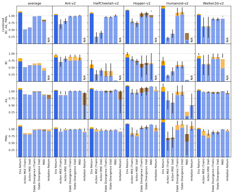
Figure 2: The episode return achieved by different algorithms if the HP selection and early stopping is performed using a proxy metric for OpenAI Gym tasks. Each subplot corresponds to a different algorithm and a different environment with the first column showing the results averaged across environments. The first row corresponds to the case when we choose HPs as well as the IL algorithm used based on the given metric. Episode returns are rescaled for each environment so that $0$ corresponds to a random policy and $1$ to the average episode return in the demonstration set. The lower (blue) part of each bar shows the episode returns in the case of no early stopping and the full bar (blue and yellow) shows the performance when using early stopping with the same metric as for the HP selection. The vertical lines show the 25-th and 75-th percentile of the episode return across reruning the whole HP selection process as described in Sec. 2.5 for the early stopping case. Brown color in the upper part of the bar means that the algorithm performs better without early stopping and shows how much performance is lost by using it. Each bar shows the mean performance across running the HP selection process 100 times.

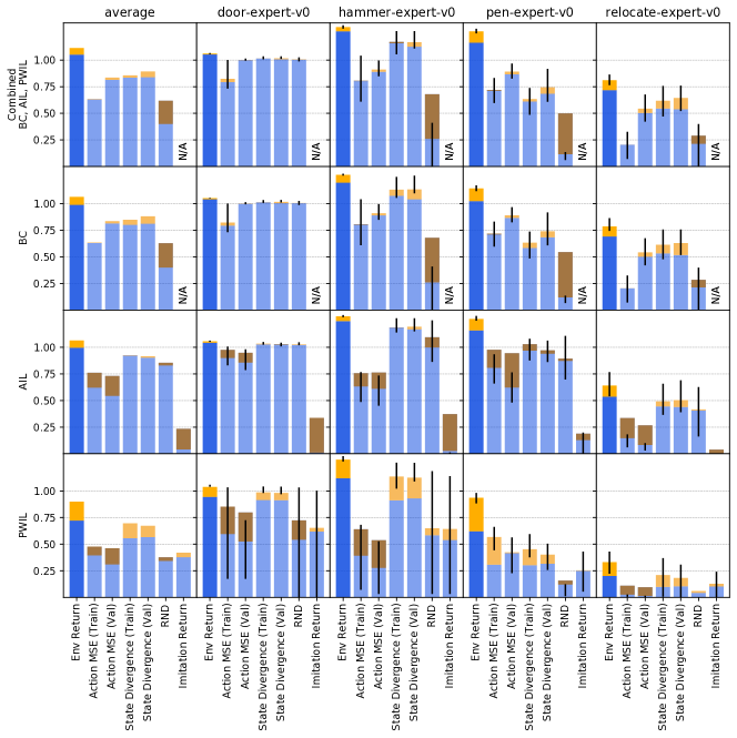
Figure 3: The episode return achieved by different algorithms if the HP selection and early stopping is performed using a proxy metric for Adroit environments. See the caption for Fig. 2 for the detailed description of this plot.

Fig. 2 and Fig. 3 show how the performance of different algorithms varies as we change the metric used for HP selection on OpenAI Gym and Adroit environments respectively.

By looking at the first bar in each subplot (performance for HPs selected on the episode return), we can see that all algorithms, including BC, can achieve returns comparable to or even better than those of the expert on almost all environments if the HP selection and early stopping are performed using the oracle episode return. In some cases, the policies obtained this way can even perform significantly better than the expert (e.g. BC on pen-expert, Fig. 3). This should not happen as all the algorithms are trying to mimic the expert behaviour and we argue that this is an artifact of the policy selection process.

How much do we lose by choosing an IL algorithm and HPs using a proxy metric? The top-left subplot in Fig. 2 and Fig. 3 shows the performance averaged across the tasks in a given suite when the HPs as well as the IL algorithm are chosen using the proxy metrics. The selection by state divergence achieves episode returns similar to that of the demonstrator on both environment suites. This is a very positive result, suggesting that it is, in practice, possible to select HPs without access to a reward function and still obtain a policy that performs well at the task.

On the other hand, the big gap between the performance of all three algorithms on Adroit (first column in Fig. 3) with HPs selected on the return vs. proxy metrics shows that the research practice of selecting HPs based on the return can lead to significant overestimation of an algorithm’s performance when no reward function is available. This may limit the applicability of some IL algorithms to practical problems.

Which proxy metric is the best? The state divergence performs best for all algorithms. Action MSE performs worse than the state divergence but still achieves at least 75% of the expert score on some algorithm-environment pairs. The inferior performance of action MSE is expected as it is a fully offline metric unaware of the system dynamics. Whether the metrics are computed against the set of training demonstrations or a held-out set of demonstrations makes little difference in our experiments and suggests that it might be better to use all available demonstrations for training.

The metric given by the average RND score on the episode performs well to select HPs on OpenAI Gym environments but is outperformed by the state divergence. Perhaps suprisingly, the metric is not as performant on Adroit. This suggests that this support-estimation metric might have to be adapted for environments with more stochasticity in initial states. Imitation return (the sum of learned-reward collected in an episode), as defined by in AIL and PWIL also perform poorly and is usually worse than action MSE with the exception of PWIL on OpenAI Gym where both approaches perform similarly. The inferior performance of the imitation return for AIL can be explained by the fact that the reward function introduced in the algorithm is non-stationary. Therefore comparing the values from different training runs or different timesteps might be misleading. Concerning PWIL, we suspect that its inferior performance on Adroit compared to the state divergence metrics is caused by the fact that the upper-bound on the Wasserstein distance introduced by the algorithm is not tight.

Is early stopping important? The upper yellow (resp. brown) parts of the bars in Fig. 2 and Fig. 3 show how much is gained (resp. lost) by using early stopping based on the same metric as for the HP selection. We can see that early stopping almost always improves performances if a reliable metric (i.e., state divergence) is used and the task was not already almost completely solved without it. The magnitude of the gain depends heavily on the environment and the algorithm, in particular we found early stopping to be particularly helpful for PWIL on Adroit environments.

Can we use metrics to choose the algorithm? The first row in Fig. 2 and Fig. 3 show the performance when we use the metrics to choose not only HPs but also the IL algorithm. We observe that when using the state divergence as the metric to select the algorithm, we achieve comparable performance to that of the best algorithm. Furthermore, selecting the algorithm based on action MSE results in similar performance as BC even if it is not the best algorithm. This may be due to the fact that BC optimizes the very same criterion, hence it is more likely to have the best results according to that metric. We provide additional evidence for this hypothesis in Appx. B.2.

3.2 Hyperparameter selection by transfer

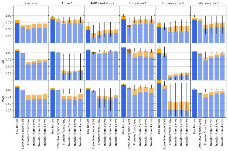
Figure 4: The episode return achieved by different algorithms if the HP selection is performed using transfer for OpenAI Gym environments. HPs are selected by choosing the HP configuration which performs best on a set of other tasks from the same benchmark (See Sec. 2.5 for the details). The results are averaged across all possible choices of the validation environments. Different bars in each subplot correspond to using a different number of environments to select HPs. We also include the selection based on the episode return and the state divergence for comparison. Early stopping is performed using the state divergence (validation) regardless of the HP selection metric. See the caption for Fig. 2 for additional information on this figure.

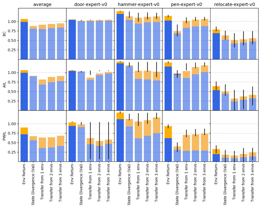
Figure 5: The episode return achieved by different algorithms if the HP selection is performed using transfer for Adroit environments. See Fig. 4 for additional information on this plot.

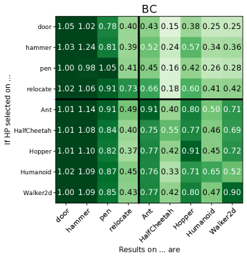
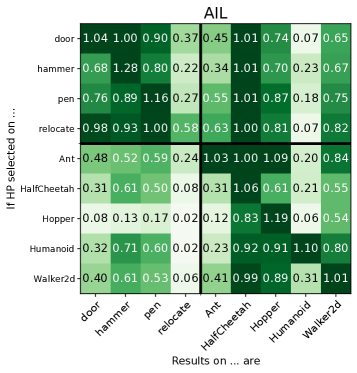
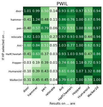
Figure 6: HP transfer results for individual validation-test environments pairs. Rows correspond to different validation environments and columns to different test environments. Early stopping is performed using the state divergence on the validation set of demonstrations.

As an alternative to the metrics investigated in the previous section, we could select HPs which work best on a similar task(s) that actually has a well-defined reward function. Fig. 4 and 5 show the performance of different algorithms when we choose HPs using a set of validation environments and then test them on another environment from the same benchmark (i.e., we do not consider the transfer from OpenAI Gym to Adroit here). While we could use transfer for early stopping (i.e., select the timestep which worked best for the validation environments), we have noticed that it almost always resulted in worse performance than no early stopping and therefore we chose to use state divergence for early stopping in the transfer experiments.

Transfer performance consistently improves with the number of validation environments used but selecting HPs based on the state divergence on the task of interest outperforms transfer even if we validate HPs on all the other tasks in the given task suite. The relatively poor transfer performance can be caused by two factors: (1) different HP configurations performing well on each task, or (2) the stochasticity of the algorithm (i.e., the algorithm producing different results when run twice with the same HPs). Despite that, transferring HPs may still be preferred in some situations as it does not require tuning HPs for each new task.

Fig. 6 shows the transfer performance for individual pairs of validation-test environments. We observe that HPs transfer better within a suite, but the HP transfer between OpenAI Gym and Adroit often succeeds too. Especially, BC’s HPs transfer very well from Adroit to Gym but not the other way around. Results also suggest that HPs transfer better to easier tasks than to harder ones: the two tasks on which the HP transfer performs worst are Humanoid and relocate which are the hardest tasks in their respective suites.

The results suggest also that BC enjoys better HP transferability than AIL and PWIL which can be expected as it is a much simpler algorithm based on supervised learning.

A general conclusion from our experiments is that IL algorithms are quite sensitive to their HPs and may require per-environment HP tuning for optimal performance. It is therefore important to compare IL algorithms not only in terms of their performance under optimal HPs but also in terms of their HP sensitivity and transferability.

4 Related Work

Hyperparameters selection is central to the performance of machine learning algorithms. In the context of supervised learning, it is common practice to select HPs on dedicated held-out data (validation) and subsequently estimate the performance of an algorithm on another set of held-out data (test). Previous work has looked into improving the selection of the best configurations using grid search (LeCun et al., 2012), random search (Larochelle et al., 2007; Bergstra & Bengio, 2012) or population based strategies (Jaderberg et al., 2017).

In the context of reinforcement learning, the notions of training and validation can be conflated. This is the case if the goal is to design a policy that performs well in a single environment (Silver et al., 2016; Tesauro, 1995; Vinyals et al., 2017). However, RL agents are typically evaluated on their ability to learn on multiple environments (Bellemare et al., 2013; Brockman et al., 2016; Cobbe et al., 2020) with a single set of HPs. Henderson et al. (2018) highlights that poor evaluation protocols make RL algorithms hard to reproduce. For instance, although code level optimizations often explain a lot of the RL algorithms performance, they tend to be omitted in most of the recent RL publications (Engstrom et al., 2020; Andrychowicz et al., 2020), making it hard for practionners to compare and reproduce.

Imitation Learning adds another level of algorithmic complexity to the RL setting since the reward function is not available. Therefore, the learning of a reward function, which introduces its own set of extra HPs, is intertwined with the learning process of a direct RL agent (Finn et al., 2016; Ho & Ermon, 2016; Kostrikov et al., 2018). Although previous work has identified measures of similarity not based on the reward functions (Dadashi et al., 2020; Ghasemipour et al., 2020; Ke et al., 2019), this work is, as far as we know, the first to propose a principled evaluation protocol to select HPs not based on the true but supposedly unknown reward function.

Paine et al. (2020) recently highlighted the same problem occurring in offline RL (Lagoudakis & Parr, 2003; Ernst et al., 2005; Riedmiller, 2005; Lange et al., 2012; Levine et al., 2020), where HPs are usually selected on the performance of the agent on the online environment (although the core constraint of offline RL prevents interactions with the environment). Some recent benchmarks (Gulcehre et al., 2020; Fu et al., 2020) also propose evaluation protocols where HPs are selected by tuning on only a subset of environments.

5 Summary/Conclusion

In this work, we highlighted a major flaw in current evaluation protocols of IL methods. Although the promise is to design agents learning from demonstrations, the standard practice is to select agents on the reward of the task. In order to align research progress with the problem it attempts to solve, we advocate for a new evaluation protocol, where the HP selection is based on criteria available in the IL setting. We investigated multiple proxies to the environment return for HP selection and early stopping. We evaluated, on 9 continuous control tasks, model selection using proxy metrics or through transfer. We demonstrated the brittleness of classical algorithms when the HP selection cannot be performed on the unknown environment return. We also showed that it is possible to select good HPs by estimating the divergence between the distribution of states encountered by the demonstrator and the agent. This work opens the interesting question of new proxy metrics design, that can adapt to harder IL settings including suboptimal demonstrations, partial observability or visual-based inputs.

Appendix A Experimental details

All experiments use MLP networks (optionally with dropout (Srivastava et al., 2014)) and Adam (Kingma & Ba, 2014) optimizer. Some experiments use observation normalization which means that the observation coordinates are rescaled to have the mean equal $0$ and standard deviation equal $1$. The normalization statistics are computed using the dataset of expert trajectories.

Both, AIL and PWIL use SAC (Haarnoja et al., 2018a) with an entropy constraint (Haarnoja et al., 2018b) to train the policy and optionally use absorbing states introduced in DAC (Kostrikov et al., 2018). When evaluating SAC policies, we decrease the stochasticity of the policy by sampling each actions 5 times and averaging the sampled actions.

A.1 Behavioral Cloning

The HP sweep for BC can be found in Table 1.

Table 1: Hyperparameter sweep for BC.

Hyperparameter	Possible values
gradient updates	6000
batch size	256
learning rate	$10^{-5}$, $10^{-4}$
weight decay coefficient	0, 0.01, 0.1
observation normalization	True, False
policy output	deterministic
# of policy hidden layers	1, 2, 3
hidden layer size	16-256
activation function	ReLU, tanh
input dropout rate	0, 0.15, 0.3
hidden dropout rate	0, 0.25, 0.5

A.2 Adversarial Imitation Learning

The HP sweep for AIL can be found in Table 2. The AIL experiment samples the policy reward function from the following options (Kostrikov et al., 2018; Ghasemipour et al., 2020):

• $\log D(s,a)$,

• $-\log(1-D(s,a))$,

• $\log D(s,a)-\log(1-D(s,a))$.

To prevent the discriminator saturation, we subtract the entropy of the discriminator output (treated as a Bernoulli distribution) from the discriminator loss.

Table 2: Hyperparameter sweep for AIL.

Hyperparameter	Possible values
discriminator training
# of gradient steps per env step	1
training batch size	256
# of hidden layers	2
hidden layer size	256
activation function	ReLU
learning rate	$10^{-6}$–$3\cdot 10^{-4}$
entropy coefficient	$10^{-4}$–$10^{-2}$
RL reward function	See App. A.2
observation normalization	True, False
absorbing states	True, False
RL training	See Table 3.

Table 3: Hyperparameter sweep for SAC.

Hyperparameter	Possible values
environment steps	1M
replay buffer size	1M
gradient steps per env step	1
learning rate	$3\cdot 10^{-5}$ – $1\cdot 10^{-3}$
batch size	128, 256, 512
discount factor	0.9, 0.97, 0.99
target network coefficient	0.001 – 0.03
reward scale	0.01 – 1
target entropy	-0.5 per dimension
policy
action distribution	Gaussian + tanh
# of hidden layers	2
hidden layer size	256
activation function	ReLU

A.3 Primal Wasserstein Imitation Learning

The hyperparameter sweep for PWIL can bew found in Table 4. PWIL prefills the SAC replay buffer with a number of transitions from the expert dataset.

Table 4: Hyperparameter sweep for PWIL.

Hyperparameter	Possible values
observation normalization	True, False
absorbing states	True, False
reward coefficient $\alpha$	0.5, 1, 5, 10
reward coefficient $\beta$	0.5, 1, 5, 10
# of expert transitions in the buffer	0, 5k, 50k
RL training	See Table 3.

A.4 Random Network Distillation metric

This metric uses a first frozen feed-forward network $f$ with layer sizes $(128,128,128,128)$ as a target and a second learnable network $\hat{f}$ with layer sizes $(128,128)$ to predict the output of the former. The latter is trained with Adam and a learning rate of $0.001$ to minimize the mean-squared error for 100 epochs on the demonstration dataset. The corresponding metric is given by $\exp(-||f(obs)-\hat{f}(obs)||)$.

Appendix B Additional results

B.1 Ranking property of the proposed metrics

Whether a metric is good for HP selection mostly depends on its capacity to preserve the ranking between policies induced by the oracle return. Assuming a set of policies whose expected return is evenly distributed over an interval, we can introduce two tasks that can serve as an intrinsic evaluation of the proxy metrics. The first task aims at ranking all the policies according to the chosen metric. The performance of this ranking is given by the Spearman correlation with the ranking provided by the oracle return. The second task aims at differentiating the set of good policies, i.e. policies whose oracle return is above a threshold (chosen to be 75% of the expert performance), from the set of poor policies: we compute the probability that the chosen metric is lower for a policy sampled randomly from the set of good policies than for a policy sampled randomly from the set of poor policies. This probability also corresponds to the ROC-AUC of a classifier that would be based on the same metric.

To create a set of policies, we train some agents using one of the IL algorithms configured as described in Sec. A and collect for each HP configuration the policies from different stages of training. The resulting set of policies is highly imbalanced in terms of environment returns. To get policies evenly distributed in terms of environment returns, we finally rebalance the set of policies. The two tasks are repeated for each set of policies obtained using BC, AIL and PWIL and the corresponding scores are averaged.

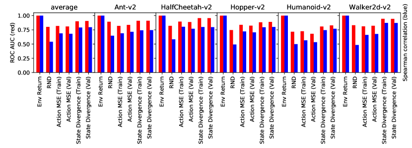
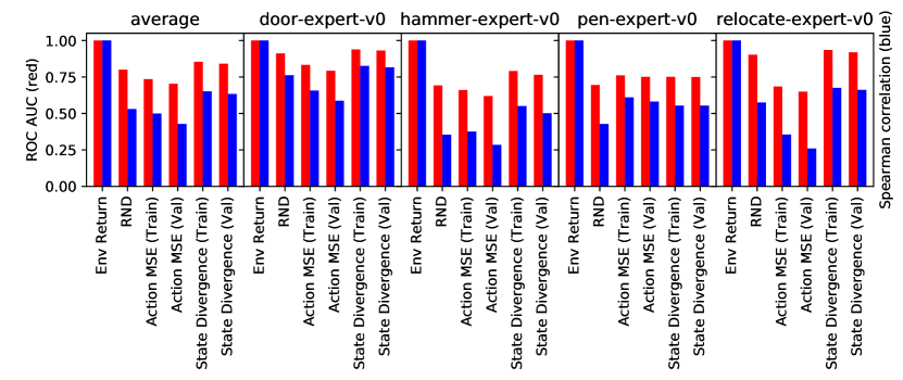
Figure 7: ROC-AUC (red) and Spearman correlation (blue) of the proposed metrics with respect to the oracle return on a set of Mujoco and D4RL adroit environments.

Fig. 7 clearly shows the metrics somewhat preserve the ranking induced by the oracle return. The best metric on those two ranking tasks is the state divergence, suggesting this could be the most suitable metric for HP selection.

B.2 Selecting the algorithm

The first row of Fig. 2 gives the episode returns for the different proposed metrics when the imitation learning algorithm is itself considered as an hyperparameter. The results suggest the action MSE metric favors BC even when BC is actually not the best algorithm. We provide in Fig. 8 an evidence of this hypothesis through a detailed view of all the partially-trained models from different HP configurations for each of the three imitation learning algorithms. The models with best action MSE correspond to models learned with BC although they are clearly not the best models in this case.

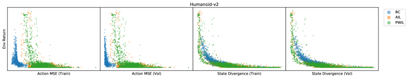
Figure 8: Values of the environment return and of the action MSE and state divergence metrics for all the models (across HPs and training steps) of the three different imitation learning algorithms.

B.3 Transfer

We include in Fig.6 the performance of algorithms when transferring HPs from one environment to another when the early stopping is performed on the state divergence as this metric was the most promising according to Sec. 3.1. We include here the results of the same experiments when early stopping is performed on the oracle return (9) or when no early stopping is performed (10).

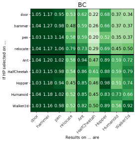
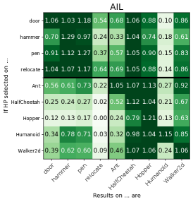
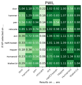
Figure 9: HP transfer results for individual validation-test environments pairs. Rows correspond to different validation environments and columns to different test environments. Early stopping is performed using the oracle return.

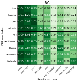
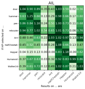
Figure 10: HP transfer results for individual validation-test environments pairs. Rows correspond to different validation environments and columns to different test environments. No early stopping is performed.

References

- Andrychowicz et al. (2020) Andrychowicz, M., Raichuk, A., Stańczyk, P., Orsini, M., Girgin, S., Marinier, R., Hussenot, L., Geist, M., Pietquin, O., Michalski, M., et al. What matters in on-policy reinforcement learning? a large-scale empirical study. arXiv preprint arXiv:2006.05990, 2020.
- Argall et al. (2009) Argall, B. D., Chernova, S., Veloso, M., and Browning, B. A survey of robot learning from demonstration. Robotics and autonomous systems, 57(5):469–483, 2009.
- Bellemare et al. (2013) Bellemare, M. G., Naddaf, Y., Veness, J., and Bowling, M. The arcade learning environment: An evaluation platform for general agents. Journal of Artificial Intelligence Research, 47:253–279, 2013.
- Bergstra & Bengio (2012) Bergstra, J. and Bengio, Y. Random search for hyper-parameter optimization. Journal of machine learning research, 13(2), 2012.
- Berner et al. (2019) Berner, C., Brockman, G., Chan, B., Cheung, V., Debiak, P., Dennison, C., Farhi, D., Fischer, Q., Hashme, S., Hesse, C., et al. Dota 2 with large scale deep reinforcement learning. arXiv preprint arXiv:1912.06680, 2019.
- Bradbury et al. (2018) Bradbury, J., Frostig, R., Hawkins, P., Johnson, M. J., Leary, C., Maclaurin, D., Necula, G., Paszke, A., VanderPlas, J., Wanderman-Milne, S., and Zhang, Q. JAX: composable transformations of Python+NumPy programs, 2018. URL http://github.com/google/jax.
- Brockman et al. (2016) Brockman, G., Cheung, V., Pettersson, L., Schneider, J., Schulman, J., Tang, J., and Zaremba, W. Openai gym. arXiv preprint arXiv:1606.01540, 2016.
- Burda et al. (2018) Burda, Y., Edwards, H., Storkey, A., and Klimov, O. Exploration by random network distillation. arXiv preprint arXiv:1810.12894, 2018.
- Cobbe et al. (2020) Cobbe, K., Hesse, C., Hilton, J., and Schulman, J. Leveraging procedural generation to benchmark reinforcement learning. In International conference on machine learning, pp. 2048–2056. PMLR, 2020.
- Dadashi et al. (2020) Dadashi, R., Hussenot, L., Geist, M., and Pietquin, O. Primal wasserstein imitation learning. arXiv preprint arXiv:2006.04678, 2020.
- Ecoffet et al. (2021) Ecoffet, A., Huizinga, J., Lehman, J., Stanley, K. O., and Clune, J. First return, then explore. Nature, 590(7847):580–586, 2021.
- Engstrom et al. (2020) Engstrom, L., Ilyas, A., Santurkar, S., Tsipras, D., Janoos, F., Rudolph, L., and Madry, A. Implementation matters in deep policy gradients: A case study on ppo and trpo. arXiv preprint arXiv:2005.12729, 2020.
- Ernst et al. (2005) Ernst, D., Geurts, P., and Wehenkel, L. Tree-based batch mode reinforcement learning. Journal of Machine Learning Research, 6:503–556, 2005.
- Feldt (1998) Feldt, R. Generating diverse software versions with genetic programming: an experimental study. IEE Proceedings-Software, 145(6):228–236, 1998.
- Finn et al. (2016) Finn, C., Levine, S., and Abbeel, P. Guided cost learning: Deep inverse optimal control via policy optimization. In International conference on machine learning, pp. 49–58. PMLR, 2016.
- Flamary & Courty (2017) Flamary, R. and Courty, N. Pot python optimal transport library, 2017. URL https://pythonot.github.io/.
- Fu et al. (2020) Fu, J., Kumar, A., Nachum, O., Tucker, G., and Levine, S. D4rl: Datasets for deep data-driven reinforcement learning. arXiv preprint arXiv:2004.07219, 2020.
- Ghasemipour et al. (2020) Ghasemipour, S. K. S., Zemel, R., and Gu, S. A divergence minimization perspective on imitation learning methods. In Conference on Robot Learning, pp. 1259–1277. PMLR, 2020.
- Gulcehre et al. (2020) Gulcehre, C., Wang, Z., Novikov, A., Paine, T. L., Colmenarejo, S. G., Zolna, K., Agarwal, R., Merel, J., Mankowitz, D., Paduraru, C., et al. Rl unplugged: Benchmarks for offline reinforcement learning. arXiv preprint arXiv:2006.13888, 2020.
- Haarnoja et al. (2018a) Haarnoja, T., Zhou, A., Abbeel, P., and Levine, S. Soft actor-critic: Off-policy maximum entropy deep reinforcement learning with a stochastic actor. In International Conference on Machine Learning, pp. 1861–1870. PMLR, 2018a.
- Haarnoja et al. (2018b) Haarnoja, T., Zhou, A., Hartikainen, K., Tucker, G., Ha, S., Tan, J., Kumar, V., Zhu, H., Gupta, A., Abbeel, P., et al. Soft actor-critic algorithms and applications. arXiv preprint arXiv:1812.05905, 2018b.
- Heek et al. (2020) Heek, J., Levskaya, A., Oliver, A., Ritter, M., Rondepierre, B., Steiner, A., and van Zee, M. Flax: A neural network library and ecosystem for JAX, 2020. URL http://github.com/google/flax.
- Henderson et al. (2018) Henderson, P., Islam, R., Bachman, P., Pineau, J., Precup, D., and Meger, D. Deep reinforcement learning that matters. In Proceedings of the AAAI Conference on Artificial Intelligence, volume 32, 2018.
- Hester et al. (2018) Hester, T., Vecerik, M., Pietquin, O., Lanctot, M., Schaul, T., Piot, B., Horgan, D., Quan, J., Sendonaris, A., Osband, I., et al. Deep q-learning from demonstrations. In Proceedings of the AAAI Conference on Artificial Intelligence, volume 32, 2018.
- Ho & Ermon (2016) Ho, J. and Ermon, S. Generative adversarial imitation learning. arXiv preprint arXiv:1606.03476, 2016.
- Hoffman et al. (2020) Hoffman, M., Shahriari, B., Aslanides, J., Barth-Maron, G., Behbahani, F., Norman, T., Abdolmaleki, A., Cassirer, A., Yang, F., Baumli, K., et al. Acme: A research framework for distributed reinforcement learning. arXiv preprint arXiv:2006.00979, 2020.
- Jaderberg et al. (2017) Jaderberg, M., Dalibard, V., Osindero, S., Czarnecki, W. M., Donahue, J., Razavi, A., Vinyals, O., Green, T., Dunning, I., Simonyan, K., et al. Population based training of neural networks. arXiv preprint arXiv:1711.09846, 2017.
- Ke et al. (2019) Ke, L., Barnes, M., Sun, W., Lee, G., Choudhury, S., and Srinivasa, S. Imitation learning as -divergence minimization. arXiv preprint arXiv:1905.12888, 2019.
- Kim et al. (2013) Kim, B., Farahmand, A.-m., Pineau, J., and Precup, D. Learning from limited demonstrations. In Advances in Neural Information Processing Systems, pp. 2859–2867, 2013.
- Kingma & Ba (2014) Kingma, D. P. and Ba, J. Adam: A method for stochastic optimization. arXiv preprint arXiv:1412.6980, 2014.
- Kostrikov et al. (2018) Kostrikov, I., Agrawal, K. K., Dwibedi, D., Levine, S., and Tompson, J. Discriminator-actor-critic: Addressing sample inefficiency and reward bias in adversarial imitation learning. arXiv preprint arXiv:1809.02925, 2018.
- Kumar (2016) Kumar, V. Manipulators and Manipulation in high dimensional spaces. PhD thesis, University of Washington, Seattle, 2016. URL https://digital.lib.washington.edu/researchworks/handle/1773/38104.
- Lagoudakis & Parr (2003) Lagoudakis, M. G. and Parr, R. Least-squares policy iteration. The Journal of Machine Learning Research, 4:1107–1149, 2003.
- Lange et al. (2012) Lange, S., Gabel, T., and Riedmiller, M. Batch reinforcement learning. In Reinforcement learning, pp. 45–73. Springer, 2012.
- Larochelle et al. (2007) Larochelle, H., Erhan, D., Courville, A., Bergstra, J., and Bengio, Y. An empirical evaluation of deep architectures on problems with many factors of variation. In Proceedings of the 24th international conference on Machine learning, pp. 473–480, 2007.
- LeCun et al. (2012) LeCun, Y. A., Bottou, L., Orr, G. B., and Müller, K.-R. Efficient backprop. In Neural networks: Tricks of the trade, pp. 9–48. Springer, 2012.
- Lee et al. (2020) Lee, K.-H., Fischer, I., Liu, A., Guo, Y., Lee, H., Canny, J., and Guadarrama, S. Predictive information accelerates learning in rl. arXiv preprint arXiv:2007.12401, 2020.
- Levine et al. (2020) Levine, S., Kumar, A., Tucker, G., and Fu, J. Offline reinforcement learning: Tutorial, review, and perspectives on open problems. arXiv preprint arXiv:2005.01643, 2020.
- Ng et al. (2000) Ng, A. Y., Russell, S. J., et al. Algorithms for inverse reinforcement learning. In Icml, volume 1, pp. 2, 2000.
- Paine et al. (2020) Paine, T. L., Paduraru, C., Michi, A., Gulcehre, C., Zolna, K., Novikov, A., Wang, Z., and de Freitas, N. Hyperparameter selection for offline reinforcement learning. arXiv preprint arXiv:2007.09055, 2020.
- Piot et al. (2013) Piot, B., Geist, M., and Pietquin, O. Learning from demonstrations: Is it worth estimating a reward function? In Joint European Conference on Machine Learning and Knowledge Discovery in Databases, pp. 17–32. Springer, 2013.
- Piot et al. (2014) Piot, B., Geist, M., and Pietquin, O. Boosted bellman residual minimization handling expert demonstrations. In Joint European Conference on Machine Learning and Knowledge Discovery in Databases, pp. 549–564. Springer, 2014.
- Pomerleau (1991) Pomerleau, D. A. Efficient training of artificial neural networks for autonomous navigation. Neural computation, 3(1):88–97, 1991.
- Popov et al. (2017) Popov, I., Heess, N., Lillicrap, T., Hafner, R., Barth-Maron, G., Vecerik, M., Lampe, T., Tassa, Y., Erez, T., and Riedmiller, M. Data-efficient deep reinforcement learning for dexterous manipulation. arXiv preprint arXiv:1704.03073, 2017.
- Riedmiller (2005) Riedmiller, M. Neural fitted q iteration–first experiences with a data efficient neural reinforcement learning method. In European Conference on Machine Learning, pp. 317–328. Springer, 2005.
- Russell (1998) Russell, S. Learning agents for uncertain environments. In Conference on Computational learning theory, 1998.
- Schaal (1999) Schaal, S. Is imitation learning the route to humanoid robots? Trends in Cognitive Sciences, 3(6):233 – 242, 1999. ISSN 1364-6613. doi: https://doi.org/10.1016/S1364-6613(99)01327-3. URL http://www.sciencedirect.com/science/article/pii/S1364661399013273.
- Silver et al. (2016) Silver, D., Huang, A., Maddison, C. J., Guez, A., Sifre, L., Van Den Driessche, G., Schrittwieser, J., Antonoglou, I., Panneershelvam, V., Lanctot, M., et al. Mastering the game of go with deep neural networks and tree search. nature, 529(7587):484–489, 2016.
- Sims (1994) Sims, K. Evolving virtual creatures. In Proceedings of the 21st annual conference on Computer graphics and interactive techniques, pp. 15–22, 1994.
- Srivastava et al. (2014) Srivastava, N., Hinton, G., Krizhevsky, A., Sutskever, I., and Salakhutdinov, R. Dropout: A simple way to prevent neural networks from overfitting. Journal of Machine Learning Research, 15(56):1929–1958, 2014. URL http://jmlr.org/papers/v15/srivastava14a.html.
- Stooke et al. (2020) Stooke, A., Lee, K., Abbeel, P., and Laskin, M. Decoupling representation learning from reinforcement learning. arXiv preprint arXiv:2009.08319, 2020.
- Tesauro (1995) Tesauro, G. Temporal difference learning and td-gammon. Communications of the ACM, 38(3):58–68, 1995.
- Villani (2008) Villani, C. Optimal transport: old and new. 2008.
- Vinyals et al. (2017) Vinyals, O., Ewalds, T., Bartunov, S., Georgiev, P., Vezhnevets, A. S., Yeo, M., Makhzani, A., Küttler, H., Agapiou, J., Schrittwieser, J., et al. Starcraft ii: A new challenge for reinforcement learning. arXiv preprint arXiv:1708.04782, 2017.
- Vinyals et al. (2019) Vinyals, O., Babuschkin, I., Czarnecki, W. M., Mathieu, M., Dudzik, A., Chung, J., Choi, D. H., Powell, R., Ewalds, T., Georgiev, P., et al. Grandmaster level in starcraft ii using multi-agent reinforcement learning. Nature, 575(7782):350–354, 2019.
- Wang et al. (2019) Wang, R., Ciliberto, C., Amadori, P. V., and Demiris, Y. Random expert distillation: Imitation learning via expert policy support estimation. In International Conference on Machine Learning, pp. 6536–6544. PMLR, 2019.
- Ziebart et al. (2008) Ziebart, B. D., Maas, A. L., Bagnell, J. A., and Dey, A. K. Maximum entropy inverse reinforcement learning. In Aaai, volume 8, pp. 1433–1438. Chicago, IL, USA, 2008.