A protocol for dynamic model calibration
Abstract
Ordinary differential equation models are nowadays widely used for the mechanistic description of biological processes and their temporal evolution. These models typically have many unknown and non-measurable parameters, which have to be determined by fitting the model to experimental data. In order to perform this task, known as parameter estimation or model calibration, the modeller faces challenges such as poor parameter identifiability, lack of sufficiently informative experimental data, and the existence of local minima in the objective function landscape. These issues tend to worsen with larger model sizes, increasing the computational complexity and the number of unknown parameters. An incorrectly calibrated model is problematic because it may result in inaccurate predictions and misleading conclusions. For non-expert users, there are a large number of potential pitfalls. Here, we provide a protocol that guides the user through all the steps involved in the calibration of dynamic models. We illustrate the methodology with two models, and provide all the code required to reproduce the results and perform the same analysis on new models. Our protocol provides practitioners and researchers in biological modelling with a one-stop guide that is at the same time compact and sufficiently comprehensive to cover all aspects of the problem.
Key words: systems biology; dynamic modelling; parameter estimation; identification; identifiability; optimisation.
Introduction
The use of dynamic models has become common practice in the life sciences. Mathematical modeling provides a rigorous, compact way of encapsulating the available knowledge about a biological process. Perhaps more importantly, it is also a tool for understanding, analysing, and predicting the behaviour of a complex system under conditions for which no experimental data are available. To these ends, it is particularly important that the model has been developed with that specific purpose in mind.
In biomedicine, dynamic models are used for basic research as well as for medical applications. On one hand, dynamic models facilitate an understanding of biological processes, e.g. by identifying from a list of alternative mechanisms the most plausible one [50]. On the other hand, dynamic models with sufficient mechanistic detail can be used to make predictions, including the selection of drug targets [67], and the outcome of individual and combination treatments [25, 36]. In bio- and process engineering, dynamic models are used to design and optimise biotechnological processes. Here, models are, for instance, used to find the genetic and regulatory modifications that enhance the production of a target metabolite while enforcing constraints on certain metabolite levels [74, 1, 91, 9]. In synthetic biology, dynamic models guide the design of artificial biological circuits where fine-tuned expression levels are necessary to ensure the correct functioning of regulatory elements [45, 39, 76, 82]. Beyond these topics, there is a broad spectrum of additional research areas.
The choice of model type and complexity depends on which biological question(s) it should address. Once this has been decided, the relevant biological knowledge is collected, e.g. from databases such as KEGG [44], STRING [80], and REACTOME [21], or from the literature. Furthermore, already available models can be used, e.g. from JWS Online [61] or Biomodels [51], and information about kinetic parameters might be extracted, e.g. from BRENDA [13] or Sabio-RK [102]. This information is used to determine the biological species and biochemical reactions that are relevant to the process. In combination with assumptions about reaction kinetics – e.g. mass action or Michaelis-Menten – these elements allow the construction of a tailored mathematical model, which will usually have nonlinear dynamics and uncertainties associated to its structure and parameter values [86]. The model can be specified in a standard format such as SBML, to take advantage of the ecosystem of tools that already support standard format [40].
The advent of high-throughput experimental techniques and the ever-growing availability of computational resources have led to the development of increasingly larger models. Common models possess tens of state variables and tens to a few hundreds of parameters (see [93, 34]). Large models can even possess thousands of state variables and parameters [25]. Dynamic models need to be calibrated, i.e. their unknown parameters have to be estimated from experimental data. In model calibration, the mismatch between simulated model output and experimental data is minimised to find the best parameter values [42, 2, 29, 64, 28]. Model calibration is a process composed of a sequence of steps, which usually need to be iterated [5] until a satisfactory result is found. It may be seen as part of a more general problem sometimes called reverse engineering [90] or (nonlinear) systems identification [70].
In this work, we consider the calibration of ordinary differential equation (ODE) models. ODE models are widely used to describe biological processes, and their calibration has been discussed in protocols for different classes of processes, including gene regulatory circuits [71], signalling networks [29], biocatalytic reactions [20], wastewater treatment [57, 103], food processing [88], biomolecular systems [85], and cardiac electrophysiology models [100]. Yet, these protocols focus on individual aspects of the calibration process (relevant for the sub-discipline) and/or lack illustration examples and codes that can be reused. The papers [57] and [103] focus on parameter subset selection via sensitivity and correlation analysis, and on subsequent model optimisation. The works of [71], [88] and [20] consider only low-dimensional models and do not provide in-depth discussion of scalability. The paper [29] neither covers structural identifiability analysis nor experimental design, and describes a prediction uncertainty approach with limited applicability. The works of [85], [100] and [20] discuss most aspects of the calibration process, but do not provide a step-by-step illustration with an example model and codes. The work of [77] is tailored to users of the MATLAB software toolbox Data2Dynamics [65].
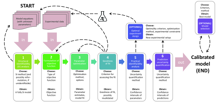
This protocol aims to provide a comprehensive description of the steps of the calibration process, which integrates recent advances. An outline of the procedure is depicted in Figure 1. The article is structured as follows. First we describe the requirements for running the calibration protocol. Then, we describe the individual steps of the protocol. The theoretical background for each step, along with a brief review of available methodologies, is provided in boxes. After some troubleshooting advice, we illustrate the application of the protocol for two case studies. For the sake of clarity, only a concise summary of the application results is reported in the main text of this manuscript; complete details are given in the supplementary information. To ensure the reproducibility of the results, we provide computational implementations used for the application of the protocol steps to the case studies in the form of MATLAB live scripts, Dockerfiles, and Python-based Jupyter notebooks.
Materials
This section describes the inputs and equipment required to run the protocol.
Hardware:
a standard personal computer, or a computer cluster. For demonstrating the application of the protocol, in the present work we have performed Step 1 on a standard laptop with a 2.40 GHz processor and 8 GB RAM. Optimisation, likelihood profiling, and sampling were performed on a laptop with an Intel Core i7-10610U CPU (eight 1.80GHz cores) and 32 GB RAM, with a total runtime of up to 2 days, per model.
Software:
a software environment with numerical computation and visualisation capabilities, along with specialised toolboxes that facilitate performing specific protocol steps. Table 1 lists the software resources used in this work.
Model:
a dynamic model described by nonlinear ODEs of the following form:
| (1) | ||||
in which is the state vector at time with initial conditions , is the output (i.e. observables) vector at time , and are possibly nonlinear functions, and is the vector of unknown parameters.
In this work we used a carotenoid pathway in Arabidopsis thaliana [11], and an EGF-dependent Akt pathway of the PC12 cell line [27], taken from the PEtab benchmark collection [34] available at https://github.com/Benchmarking-Initiative/Benchmark-Models-PEtab. An illustration of both models is provided in panels A of Fig. 5 and Fig. 6.
Data:
a set of time-resolved measurements of the model outputs. In the present work, data was taken from the aforementioned PEtab benchmark collection.
| Name | Type | Steps | Reference | Website | Environment |
|---|---|---|---|---|---|
| MATLAB | environment | all | http://www.mathworks.com | ||
| Python | environment | all | https://www.python.org | ||
| SBML | model format | input | [40] | http://www.sbml.org | MATLAB, Python |
| PEtab | data format | input | [69] | https://github.com/PEtab-dev/PEtab | Python |
| STRIKE-GOLDD | tool (SI analysis) | 1 | [95] | https://github.com/afvillaverde/strike-goldd | MATLAB |
| AMICI | tool (simulation) | 2 | [24] | https://github.com/AMICI-dev/AMICI | Python |
| pyPESTO | tool (various steps) | 3, 5, 6 | [75, 68] | https://github.com/ICB-DCM/pyPESTO | Python |
| Fides | tool (param. optimisation) | 3, 5 | [23] | https://github.com/fides-dev/fides | Python |
| SciPy | tool (various steps) | 3, 5 | [96] | https://www.scipy.org | Python |
| Data2Dynamics | tool (various steps) | 3, 5, 6, (O) | [65] | http://www.data2dynamics.org | MATLAB |
Procedure
The protocol consists of six main steps, numbered 1–6, which consist of sub-steps. Furthermore, we describe two optional steps. The workflow is depicted in Fig. 1 and described in the following paragraphs.
STEP 1: Structural identifiability analysis
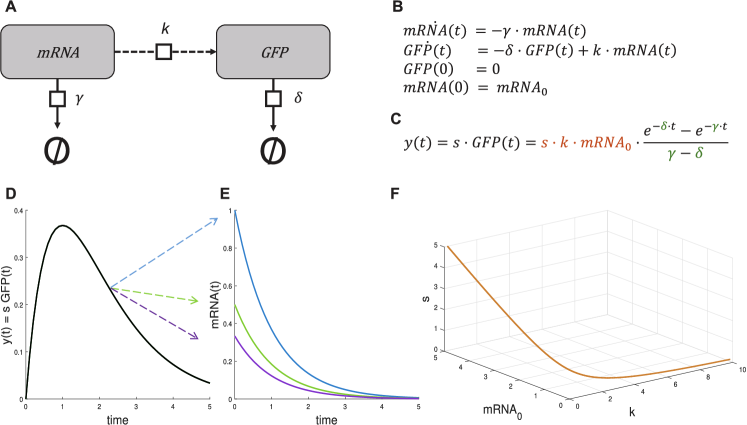
Structural identifiability is analysed to assess whether the values of all unknown parameters can be determined from perfect continuous-time and noise-free measurements of the observables under the given set of experimental conditions [99, 17]. Structural non-identifiabilities imply that there are several model parameterizations, e.g. due to symmetries or redundancies in the model structure, which yield exactly the same observables. An overview of the available methodologies for structural identifiability analysis is provided in Box 1. Fig. 2 illustrates possible sources of structural non-identifiability and the related issues. The structural identifiability analysis can be complemented by observability analysis, which determines if the trajectory of the model state can be uniquely determined from the observables.
[!htbp]
The first step in the protocol is thus:
STEP 1.1
Analyse the structural identifiability of the model with one of the methods described in Box 1.
If all parameters are structurally identifiable and all state variables are observable, we continue with Step 2.1. Otherwise, we recommend to determine the source of the structural non-identifiability as an intermediate step (1.2). Ideally, the parametric form of the non-identifiable manifold (i.e. the set of parameters that yield identical observables) is determined. Some tools offer this functionality or at least provide hints.
STEP 1.2
If parameters are structurally non-identifiable or state variables unobservable, use knowledge about the structure of the non-identifiable manifold to
-
•
reformulate the model by merging the non-identifiable parameters into identifiable combinations, OR
-
•
fix the non-identifiable parameters to reasonable values.
In both cases, the information about the non-identifiability needs to be retained to later perform a proper analysis of the prediction uncertainties. If this point is not taken into account, the obtained results are only valid for the reformulated model, but not for the original one – a fact that is often disregarded.
An alternative to the reformulation of the model or the fixing of parameters is to plan additional experiments, if possible. These can be experiments with new experimental conditions, new observables, or both (keeping experimental constraints in mind). The additional information should be recorded such that more, ideally all, parameters are structurally identifiable.
STEP 2: Formulation of objective function
The objective function measuring the mismatch of simulated model observables and measurement data is defined. The choice of the objective function depends on the characteristics of the measurement technique and accounts for knowledge about its accuracy. Possible choices are discussed in Box 2.
STEP 2.1
Construct an objective function.
[!htbp]
STEP 3: Parameter optimisation
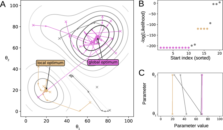
Parameter estimates are obtained by minimising the objective function. To this end, numerical optimisation methods suited for nonlinear problems with local minima should be employed. Available methodologies and practical tips for their application are discussed in Box 3, and key aspects are illustrated in Fig. 3.
STEP 3.1
Launch multiple runs of local, global, or hybrid optimisation algorithms. The number of runs required is model-dependent. For an initial optimisation we recommend at least 50 runs with purely local searches, or at least 10 runs with global or hybrid searches.
Accurate gradient computation is required for gradient-based optimisation. Before optimisation, check that the gradients appear correct by evaluating the gradient at a point, and then compare this with forward, backward, and central finite difference approximations of the gradient that are evaluated with different step sizes. Such a gradient check is a common, possibly optional, feature of tools that provide gradient-based optimisation.
STEP 3.2
Evaluate the reproducibility of the fitting results by comparing the optimal objective function values achieved by different runs. The optimal objective function values should be robustly reproducible, meaning that a substantial number of runs (rule-of-thumb: 5) should find it. If this is not the case, repeat Step 3.1 with a larger number of runs. Note that the difference between runs that is considered negligible should be statistically motivated. For the use of log-likelihood and log-posterior this corresponds to an absolute difference, not a relative one [34].
[!htbp]
STEP 4: Goodness of fit
The quality of the fitted model should be assessed by visual inspection. It is also possible to use quantitative metrics for this purpose. Details are provided in Box 4.
[!htbp]
STEP 4.1
Assess the goodness of the fit achieved by the parameter optimisation procedure.
If the fit is not good, further action is required. Proceed to STEP 4.2.
STEP 4.2
If the fit is not good enough, check convergence of the optimisation methods.
-
1.
If there are hints that searches were stopped prematurely (e.g. error messages that indicate that local optimisations did not converge), go back to STEP 3: modify the settings of the optimisation algorithms (e.g. increase maximum allowed time and/or number of evaluations) and run the optimisations again.
-
2.
If there are no signs of a premature stop, the problem may be that the optimal solution lies outside the initially chosen parameter bounds go back to STEP 3: set larger parameter bounds and run the optimisations again.
-
3.
If the actions above do not solve the issue, it may be because the optimisation method is not well suited for the problem go back to STEP 3: choose a different method and run the optimisations again.
If the new optimisations performed in STEP 4.2 do not yet yield a good fit, there may be a problem with the choice of objective function. Proceed to STEP 4.3.
STEP 4.3
If the fit is not good enough, go back to STEP 2 and select a different objective function.
If the new optimisation results are still inappropriate, the problem might be the model structure. Proceed to STEP 4.4.
STEP 4.4
If the fit is not good enough, go back to the model equations and perform a model refinement.
STEP 5: Practical identifiability analysis
[!htbp]
The task of quantifying the uncertainty in parameter estimates is known as practical (or numerical) identifiability analysis. It involves calculating univariate confidence intervals or multivariate confidence regions for the parameter values. Key concepts and tools for practical identifiability analysis are listed in Box 5. Practical identifiability issues are illustrated in Figures 5D and 6D.
STEP 5.1
Perform practical identifiability analysis with one of the methods described in Box 5. If large uncertainties in parameter estimates are revealed, then proceed to STEP 5.2.
STEP 5.2
If there are large uncertainties, then:
-
1.
If it is possible to perform new experiments add more experimental data. In this case, the experiment should be optimally designed in order to yield maximally informative data. This is described in the following section.
-
2.
If it is not possible to perform new experiments assess the possibility of simplifying the model parameterisation without losing biological interpretability.
-
3.
If neither (1) nor (2) are possible include prior knowledge about parameter values. Such information (either about the value of a parameter or about its bounds) can sometimes be found in publicly available databases.
After performing one of the above actions, go back to STEP 3.
(OPTIONAL STEP): Alternative experimental design for parameter estimation
If practical identifiability analysis concludes that there are large uncertainties in the parameter estimates, a solution may be to collect new data. Ideally, it should be obtained by designing and performing new experiments in an optimal way. Optimal Experiment Design (OED) seeks to maximise the information content of the new experiments. It can be performed using optimisation techniques that minimise an objective function that represents some measure of the uncertainty in the parameters. It is also possible to perform OED for other goals, such as model discrimination or decreasing prediction uncertainty. OED techniques are discussed in Box (O).
[!htbp]
STEP O.1
Define the constraints of the new experimental setup, and, in case of optimal design, the criterion to optimise.
STEP O.2
Obtain a new set of experiments, either by optimisation or from an educated guess.
STEP O.3
Perform experiments and collect data.
STEP O.4
Include the new data in the objective function and repeat STEPS 2–5.
STEP 6: Prediction uncertainty quantification
If the calibrated model is used for making predictions, for example about the time course of its states, it is useful to assess the prediction uncertainty. This assessment is not trivial because uncertainty in parameters does not directly translate to uncertainty in predictions. Hence it is pertinent to quantify to which extent the uncertainty in model parameters leads to uncertainty in the predictions of state trajectories. Note that, if some parameters were fixed in STEP 1 to achieve structural identifiability, in this step their values have to be altered across the plausible regime to obtain realistic confidence intervals of the state predictions. The available methods for prediction uncertainty quantification are reviewed in Box 6. Their application to case studies is shown in Fig. 5E and Fig. 6E.
[!htbp]
STEP 6.1
Calculate confidence intervals for the time courses of the predicted quantities of interest using one of the methods in Box 6.
(OPTIONAL STEP): Model selection
The protocol presented so far assumes that the model structure is known, except for the specific values of the parameters. Sometimes the form of the dynamic equations that define the model – and not only the parameter values – is not completely known a priori, and a family of candidate models may be considered. Model selection techniques choose the best model from the set of possible ones, aiming at a balance between model complexity and goodness of fit. They are discussed in Box (MS).
[!htbp]
Troubleshooting
Troubleshooting advice can be found in Table 2.
| Step | Problem | Possible reason | Solution |
|---|---|---|---|
| 1 | It is not feasible to analyse structural identifiability due to computational limitations | The model is too large and/or too complex | (A) Reduce the model complexity by fixing several parameters (conservative approach) (B) Use a numerical method (e.g. PL) to analyse practical identifiability as a proxy of structural identifiability |
| 3 | Parameter optimisation takes very long | The size of the model makes this step computationally very expensive | Use parallel optimisation approaches to decrease computation times, or try a different optimiser |
| 4 | Parameter optimisation does not result in a good fit | (A) The optimiser was stuck in a local minimum | (A) Use a global method and allow for enough time to reach the global optimum |
| (B) The parameter bounds are too small | (B) Set larger bounds | ||
| (C) The model is not an adequate representation of the system | (C) Modify the model structure | ||
| In general: use hierarchical optimisation if applicable | |||
| 4 | Parameter optimisation resulted in overfitting | Fitting the noise rather than the signal: very good calibration result that however generalises poorly | Use cross-validation to detect overfitting. If present: (A) Use regularisation in the calibration; (B) Simplify overparameterised models |
| 5 | The confidence intervals of the parameters are very large | The data are not sufficiently informative to constrain the values of the parameters sufficiently | (A) Add prior knowledge about parameter values and repeat the optimisation (B) Obtain new experimental data (ideally through OED) and repeat the optimisation |
| 6 | The confidence intervals of the predictions are very large | The data are not sufficiently informative to constrain the values of the predictions sufficiently | (Same as the above solution) |
Examples
Carotenoid pathway model
Our first case study is the carotenoid pathway model by Bruno et al. [11], with 7 states, 13 parameters, and no inputs. The model output differs among the experimental conditions: in each of the six experimental conditions for which data is available, only one of the 7 state variables is measured (one is measured in two experiments, and two states are never measured).
The application of the protocol is summarised in the following paragraphs, and the main results are shown in Fig. 5.
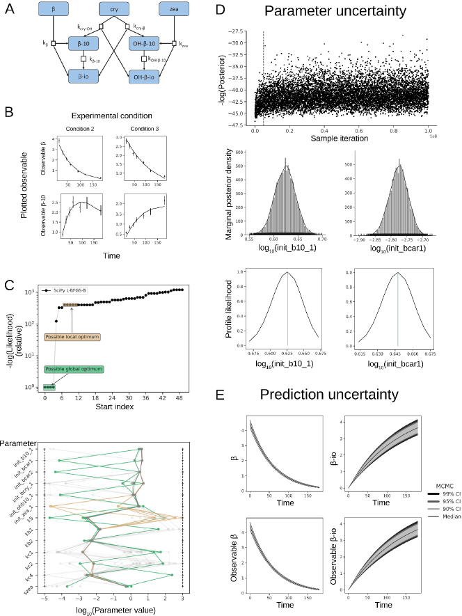
STEP 1.1: Structural identifiability analysis
We first assess structural identifiability and observability for each individual experimental condition, obtaining a different subset of identifiable parameters for each one. Next, we repeat the analysis after combining the information from all experiments, obtaining that all parameters are structurally identifiable. However, the two state variables that are not measured in any experiment (-io and OH--io) are not observable. If the initial conditions of these two states were considered as unknown parameters, they would be non-identifiable.
STEP 1.2: Address structural non-identifiabilities
We are not interested in the two unobservable states. Hence we omit this step, and proceed with the original model.
STEP 2.1: Objective function
We use the negative log-likelihood objective function described in Equation 2, which is the common choice in frequentist approaches.
STEP 3.1 and 3.2: Parameter optimisation
We estimate model parameters using the multi-start local optimisation method L-BFGS-B implemented in the Python package SciPy. With 100 starting points we achieve convergence to the maximum likelihood estimate, as indicated in the waterfall plot (Fig. 5). The parameters plot shows that the parameter vector is similar amongst the best starts, indicating that the parameters are well-determined by the optimisation problem and the optimiser.
STEP 4.1: Assess goodness of fit
Visual inspection indicates a good quality of the fit, with simulations closely matching measurements.
STEP 4.2: Address fit issues
As the fit is good, this step is skipped.
STEP 5.1: Practical identifiability analysis
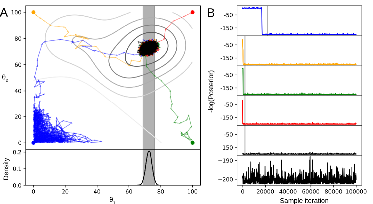
We analyse practical identifiability using profile likelihoods and MCMC sampling. Profile likelihoods suggest that all parameters are practically identifiable, as the confidence intervals span relatively small regions of the parameter space. The profiles peak at the maximum likelihood estimate (MLE), suggesting that optimisation was successful. MCMC sampling yields similar results; parameter marginal distributions span a similar distance of parameter space compared to profile likelihoods, and credibility intervals are also similar.
STEP 6.1: Prediction uncertainty analysis
We calculate credibility intervals using ensembles of parameters from sampling. In this model, there is a one-to-one correspondence between states and observables, hence the plots are the same. The prediction uncertainties are reasonably low, suggesting that the model has been successfully calibrated and might be used to predict new behaviour.
Akt pathway model
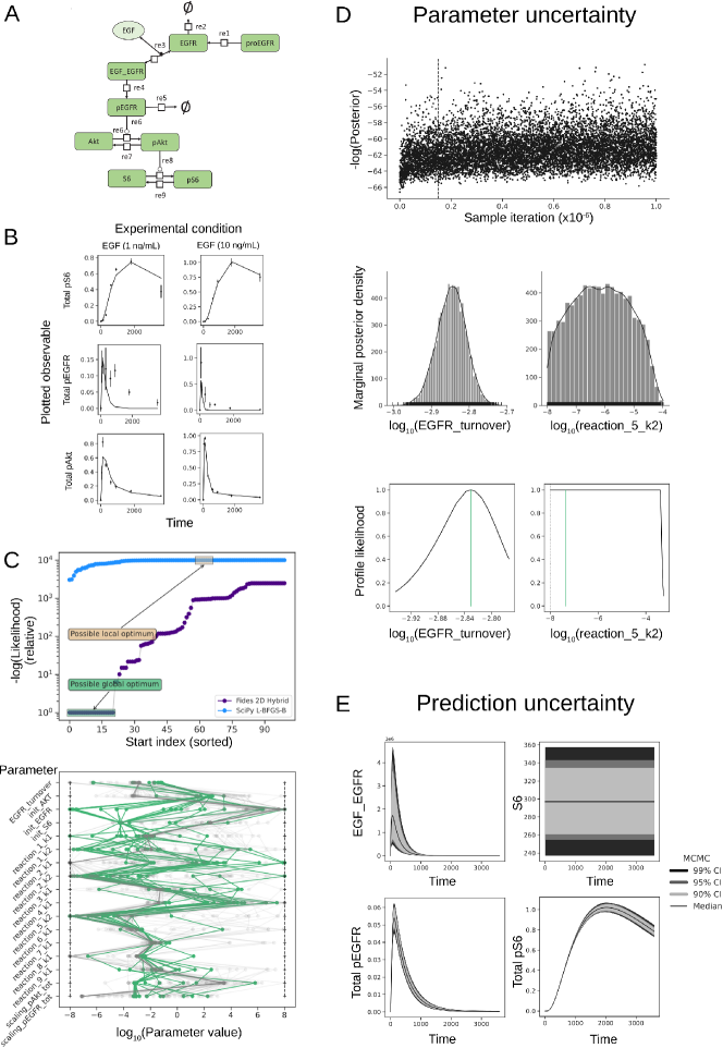
The second example is an AKT pathway model [27] with 22 unknown parameters, 3 of which are unknown initial conditions, 9 state variables, 3 outputs, and 1 input. There are 6 experimental conditions, each of them with a different input EGF concentration.
Results are summarised in the following paragraphs and in Fig. 6.
STEP 1.1: Structural identifiability analysis
We consider the following scenarios:
-
1.
For a single experiment with constant EGF, 11 parameters are structurally non-identifiable, and 3 states are unobservable.
-
2.
For a single experiment with time-varying EGF, the model becomes structurally identifiable and observable.
-
3.
For multiple experiments (at least two) with constant EGF, the model is structurally identifiable and observable.
The experimental data available corresponds to the scenario (3) above. The scenario (2) yields an identifiable and observable model, but it requires a continuously varying value of EGF, which is not practical. It is also interesting to note the role of initial conditions in this case study. The results summarised above are obtained with generic (nonzero) initial conditions. However, in the available experimental datasets there are several initial conditions equal to zero. Introducing this assumption in the analyses of the scenarios (2) and (3) leads to a loss of identifiability and observability: four parameters become non-identifiable and one state becomes unobservable.
STEP 1.2: Address structural non-identifiabilities
We assume a realistic scenario corresponding to the available experimental data: several experimental conditions with a constant input, EGF, and certain initial conditions equal to zero. In this case the model has four non-identifiable parameters and one unobservable state. To make the model fully observable and structurally identifiable, it is necessary and sufficient to fix the value of two of the non-identifiable parameters. Thus, we fix two of these parameters and proceed with the next steps.
For comparison, we also performed the remaining steps without fixing the non-identifiable parameters. We found that fixing the non-identifiability issues resulted in slightly faster and more robustly convergent optimisations, as well as in better practical identifiability and reduced state uncertainty.
STEP 2.1: Objective function
We choose the negative log-likelihood objective function described in Equation 2.
STEP 3.1 and 3.2: Parameter optimisation
Similarly to the other case study, we initially use the multi-start local optimisation method “L-BFGS-B”.
STEP 4.1: Assess goodness of fit
Visual inspection (i.e. comparison of the simulations produced by the maximum likelihood estimate with the measurements) reveals a poor fit to the data (not shown). This result is obtained even with the best result obtained from thousands of optimisation runs from different starting points.
STEP 4.2: Address fit issues
First we try to improve the fit by tuning the settings of the optimisation method, L-BFGS-B, without success. Then we try a different method, Fides, which has a higher computational cost but achieves higher quality steps during optimisation. With Fides we find an MLE that produces a fit comparable to the one reported in the original publication. The high number of starts (in the order of ) required to find this fit reproducibly indicates that this is a difficult parameter optimisation problem.
STEP 5.1: Practical identifiability analysis
Credibility intervals obtained from MCMC sampling indicate that several parameters are practically non-identifiable. This result is not significantly improved by fixing parameters as suggested in STEP 1.2. Improving the practical identifiability of these parameters would require repeating the calibration with additional experimental data.
STEP 6.1: Prediction uncertainty analysis
Credibility intervals obtained from MCMC sampling indicate that the uncertainties in the observable trajectories are reasonably low. However, the state trajectories have larger uncertainties, which make this calibrated model unsuitable for predictions involving these states. The quality of the predictions can be improved by reducing practical non-identifiabilities in the model, as mentioned in the previous step.
Discussion and conclusion
In this paper we have proposed a pipeline of methods and resources for calibrating ODE models in the context of biological applications. Its end goal is to obtain a model that is capable of making predictions about quantities of interest with quantifiable uncertainty.
The pipeline consists of a series of steps, each of which represents a task that should be fulfilled before proceeding to the next one to ensure a successful calibration. Performing these tasks entails applying computational methods of different types, symbolic and numerical. The analyses and calculations can be computationally challenging in practice. While the protocol is not dependent on a particular choice of software, we have recommended a number of state-of-the-art tools that implement the methods.
To facilitate the application of the protocol by novices as well as by experienced modellers, we have described in detail how to perform each of the protocol steps. We have also provided the theoretical background required for understanding the underlying problems. Furthermore, we have illustrated its use with two case studies: a carotenoid pathway model in Arabidopsis thaliana, and an EGF-dependent Akt pathway of the PC12 cell line. Finally, we have highlighted some of the most common pitfalls in biological modelling, showing how to avoid them.
Key Points
-
•
The correct calibration of dynamic models is essential for obtaining correct predictions and insights.
-
•
While a wide range of tools and resources are currently available, there are also many potential pitfalls, even for the expert.
-
•
Here we propose a model calibration protocol that covers all aspects of the problem.
-
•
The present paper guides the user through all the steps of the pipeline, providing a one-stop guide that is at the same time compact and comprehensive.
-
•
We provide all the code required to reproduce the results and perform the same analysis on new models, so that the biological modelling community can benefit from this pipeline.
Supplementary data
All data, scripts, and examples presented in this paper can be downloaded from:
https://github.com/ICB-DCM/model˙calibration˙protocol˙preprint.
Funding
This project has received funding from the European Union’s Horizon 2020 research and innovation programme under grant agreement No 686282 (“CANPATHPRO”). JRB also acknowledges funding from the Spanish MINECO/FEDER project SYNBIOCONTROL (DPI2017-82896-C2-2-R). AFV was partially supported by a Ramón y Cajal Fellowship (RYC-2019-027537-I) from the Spanish Ministry of Science, Innovation and Universities. Funding was received from the Deutsche Forschungsgemeinschaft (DFG, German Research Foundation) under Germany’s Excellence Strategy (EXC 2151 - 390873048: JH; EXC-2047/1 - 390685813: DP), and the German Federal Ministry of Economic Affairs and Energy (Grant no. 16KN074236: DP).
References
- [1] J. Almquist, M. Cvijovic, V. Hatzimanikatis, J. Nielsen, and M. Jirstrand. Kinetic models in industrial biotechnology–improving cell factory performance. Metab. Eng., 24:38–60, 2014.
- [2] M. Ashyraliyev, Y. Fomekong-Nanfack, J. Kaandorp, and J. Blom. Systems biology: parameter estimation for biochemical models. FEBS J., 276(4):886–902, 2009.
- [3] B. Ballnus, S. Schaper, F. J. Theis, and J. Hasenauer. Bayesian parameter estimation for biochemical reaction networks using region-based adaptive parallel tempering. Bioinformatics, 34(13):i494–i501, 2018.
- [4] E. Balsa-Canto, A. Alonso, and J. Banga. Computational procedures for optimal experimental design in biological systems. IET Syst. Biol., 2(4):163–172, 2008.
- [5] E. Balsa-Canto, A. Alonso, and J. Banga. An iterative identification procedure for dynamic modeling of biochemical networks. BMC Syst. Biol., 4:11, 2010.
- [6] J. R. Banga and E. Balsa-Canto. Parameter estimation and optimal experimental design. Essays Biochem., 45:195–210, 2008.
- [7] H. G. Bock, S. Körkel, and J. P. Schlöder. Parameter estimation and optimum experimental design for differential equation models. In Model based parameter estimation, pages 1–30. Springer, 2013.
- [8] H. Bozdogan. Model selection and akaike’s information criterion (aic): The general theory and its analytical extensions. Psychometrika, 52(3):345–370, 1987.
- [9] C. Briat and M. Khammash. Perfect adaptation and optimal equilibrium productivity in a simple microbial biofuel metabolic pathway using dynamic integral control. ACS synthetic biology, 7(2):419–431, 2018.
- [10] K. S. Brown, C. C. Hill, G. A. Calero, C. R. Myers, K. H. Lee, J. P. Sethna, and R. A. Cerione. The statistical mechanics of complex signaling networks: nerve growth factor signaling. Physical biology, 1(3):184, 2004.
- [11] M. Bruno, J. Koschmieder, F. Wuest, P. Schaub, M. Fehling-Kaschek, J. Timmer, P. Beyer, and S. Al-Babili. Enzymatic study on atccd4 and atccd7 and their potential to form acyclic regulatory metabolites. Journal of experimental botany, 67(21):5993–6005, 2016.
- [12] F. P. Casey, D. Baird, Q. Feng, R. N. Gutenkunst, J. J. Waterfall, C. R. Myers, K. S. Brown, R. A. Cerione, and J. P. Sethna. Optimal experimental design in an epidermal growth factor receptor signalling and down-regulation model. IET systems biology, 1(3):190–202, 2007.
- [13] A. Chang, I. Schomburg, S. Placzek, L. Jeske, M. Ulbrich, M. Xiao, C. W. Sensen, and D. Schomburg. Brenda in 2015: exciting developments in its 25th year of existence. Nucleic acids research, page gku1068, 2014.
- [14] M. N. Chatzis, E. N. Chatzi, and A. W. Smyth. On the observability and identifiability of nonlinear structural and mechanical systems. Struct. Control Health Monit., 22(3):574–593, 2015.
- [15] O. Chis, J. Banga, and E. Balsa-Canto. Structural identifiability of systems biology models: A critical comparison of methods. PLoS ONE, 6(11), 2011.
- [16] H. Cramér. Mathematical Methods of Statistics (PMS-9), volume 9. Princeton university press, 2016.
- [17] J. DiStefano III. Dynamic systems biology modeling and simulation. Academic Press, 2015.
- [18] B. Efron and C. Stein. The jackknife estimate of variance. The Annals of Statistics, pages 586–596, 1981.
- [19] B. Efron and R. Tibshirani. Bootstrap methods for standard errors, confidence intervals, and other measures of statistical accuracy. Statistical science, pages 54–75, 1986.
- [20] I. Eisenkolb, A. Jensch, K. Eisenkolb, A. Kramer, P. C. Buchholz, J. Pleiss, A. Spiess, and N. E. Radde. Modeling of biocatalytic reactions: A workflow for model calibration, selection and validation using bayesian statistics. AIChE Journal, 2019.
- [21] A. Fabregat, S. Jupe, L. Matthews, K. Sidiropoulos, M. Gillespie, P. Garapati, R. Haw, B. Jassal, F. Korninger, B. May, et al. The reactome pathway knowledgebase. Nucleic acids research, 46(D1):D649–D655, 2017.
- [22] G. Franceschini and S. Macchietto. Model-based design of experiments for parameter precision: State of the art. Chemical Engineering Science, 63(19):4846–4872, 2008.
- [23] F. Froehlich and P. K. Sorger. Fides: Reliable trust-region optimization for parameter estimation of ordinary differential equation models. bioRxiv, page 2021.05.20.445065, 2021.
- [24] F. Fröhlich, B. Kaltenbacher, F. J. Theis, and J. Hasenauer. Scalable parameter estimation for genome-scale biochemical reaction networks. PLOS Computational Biology, 13(1):e1005331, 2017.
- [25] F. Fröhlich, T. Kessler, D. Weindl, A. Shadrin, L. Schmiester, H. Hache, A. Muradyan, M. Schütte, J.-H. Lim, M. Heinig, et al. Efficient parameter estimation enables the prediction of drug response using a mechanistic pan-cancer pathway model. Cell systems, 7(6):567–579, 2018.
- [26] F. Fröhlich, F. J. Theis, and J. Hasenauer. Uncertainty analysis for non-identifiable dynamical systems: Profile likelihoods, bootstrapping and more. In International Conference on Computational Methods in Systems Biology, pages 61–72. Springer, 2014.
- [27] K. A. Fujita, Y. Toyoshima, S. Uda, Y.-i. Ozaki, H. Kubota, and S. Kuroda. Decoupling of receptor and downstream signals in the akt pathway by its low-pass filter characteristics. Science Signaling, 3(132):ra56–ra56, 2010.
- [28] K. Gadkar, D. Kirouac, D. Mager, P. H. van der Graaf, and S. Ramanujan. A six-stage workflow for robust application of systems pharmacology. CPT: Pharmacometrics & Systems Pharmacology, 5(5):235–249, 2016.
- [29] F. Geier, G. Fengos, F. Felizzi, and D. Iber. Analyzing and Constraining Signaling Networks: Parameter Estimation for the User. In X. Liu and M. D. Betterton, editors, Computational Modeling of Signaling Networks, volume 880 of Methods in Molecular Biology, pages 23–40. Humana Press, Totowa, NJ, 2012.
- [30] M. Gevers. Identification for control: From the early achievements to the revival of experiment design. European journal of control, 11(4-5):335–352, 2005.
- [31] J. Hadamard. Sur les problèmes aux dérivées partielles et leur signification physique. Princeton university bulletin, pages 49–52, 1902.
- [32] D. R. Hagen, J. K. White, and B. Tidor. Convergence in parameters and predictions using computational experimental design. Interface Focus, 3(4):20130008, 2013.
- [33] H. Hass, C. Kreutz, J. Timmer, and D. Kaschek. Fast integration-based prediction bands for ordinary differential equation models. Bioinformatics, 32(8):1204–1210, 2015.
- [34] H. Hass, C. Loos, E. Raimúndez-Álvarez, J. Timmer, J. Hasenauer, and C. Kreutz. Benchmark problems for dynamic modeling of intracellular processes. Bioinformatics, 35(17):3073–3082, 2019.
- [35] S. Hengl, D. Kreutz, J. Timmer, and T. Maiwald. Data-based identifiability analysis of non-linear dynamical models. Bioinformatics, 23(19):2612–2618, 2007.
- [36] D. Henriques, A. F. Villaverde, M. Rocha, J. Saez-Rodriguez, and J. R. Banga. Data-driven reverse engineering of signaling pathways using ensembles of dynamic models. PLOS Computational Biology, 2017.
- [37] H. Hong, A. Ovchinnikov, G. Pogudin, and C. Yap. Sian: software for structural identifiability analysis of ode models. Bioinformatics, 35(16):2873–2874, 2019.
- [38] S. Hross and J. Hasenauer. Analysis of cfse time-series data using division-, age-and label-structured population models. Bioinformatics, 32(15):2321–2329, 2016.
- [39] V. Hsiao, A. Swaminathan, and R. M. Murray. Control theory for synthetic biology: Recent advances in system characterization, control design, and controller implementation for synthetic biology. IEEE Control Systems, 38(3):32–62, 2018.
- [40] M. Hucka, A. Finney, H. Sauro, H. Bolouri, and J. Doyle. The systems biology markup language (sbml): A medium for representation and exchange of biochemical network models. Bioinformatics, 19:524–531, 2003.
- [41] S. Hug, A. Raue, J. Hasenauer, J. Bachmann, U. Klingmüller, J. Timmer, and F. Theis. High-dimensional bayesian parameter estimation: case study for a model of jak2/stat5 signaling. Mathematical Biosciences, 246(2):293–304, 2013.
- [42] K. Jaqaman and G. Danuser. Linking data to models: data regression. Nat. Rev. Mol. Cell Bio., 7(11):813–819, 2006.
- [43] M. Joshi, A. Seidel-Morgenstern, and A. Kremling. Exploiting the bootstrap method for quantifying parameter confidence intervals in dynamical systems. Metab. Eng., 8:447–455, 2006.
- [44] M. Kanehisa and S. Goto. Kegg: kyoto encyclopedia of genes and genomes. Nucleic acids research, 28(1):27–30, 2000.
- [45] E. Karamasioti, C. Lormeau, and J. Stelling. Computational design of biological circuits: putting parts into context. Molecular Systems Design & Engineering, 2(4):410–421, 2017.
- [46] J. Karlsson, M. Anguelova, and M. Jirstrand. An efficient method for structural identiability analysis of large dynamic systems. In 16th IFAC Symposium on System Identification, volume 16, pages 941–946, (2012).
- [47] C. Kreutz. New concepts for evaluating the performance of computational methods. IFAC-PapersOnLine, 49(26):63–70, 2016.
- [48] C. Kreutz, A. Raue, D. Kaschek, and J. Timmer. Profile likelihood in systems biology. The FEBS journal, 280(11):2564–2571, 2013.
- [49] C. Kreutz, A. Raue, and J. Timmer. Likelihood based observability analysis and confidence intervals for predictions of dynamic models. BMC Systems Biology, 6(1):120, 2012.
- [50] L. Kuepfer, M. Peter, U. Sauer, and J. Stelling. Ensemble modeling for analysis of cell signaling dynamics. Nature biotechnology, 25(9):1001–1006, 2007.
- [51] N. Le Novère, B. Bornstein, A. Broicher, M. Courtot, M. Donizelli, H. Dharuri, L. Li, H. Sauro, M. Schilstra, B. Shapiro, J. L. Snoep, and M. Hucka. BioModels Database: a free, centralized database of curated, published, quantitative kinetic models of biochemical and cellular systems. Nucleic Acids Research, 34(Database issue):D689–D691, Jan 2006.
- [52] J. Li. Assessing the accuracy of predictive models for numerical data: Not r nor r2, why not? then what? PLOS ONE, 12(8):e0183250, Aug. 2017.
- [53] J. Liepe, P. Kirk, S. Filippi, T. Toni, C. P. Barnes, and M. P. Stumpf. A framework for parameter estimation and model selection from experimental data in systems biology using approximate bayesian computation. Nature protocols, 9(2):439–456, 2014.
- [54] T. S. Ligon, F. Fröhlich, O. T. Chiş, J. R. Banga, E. Balsa-Canto, and J. Hasenauer. Genssi 2.0: multi-experiment structural identifiability analysis of sbml models. Bioinformatics, 34(8):1421–1423, 2017.
- [55] D. Lopez, T. Barz, S. Körkel, G. Wozny, et al. Nonlinear ill-posed problem analysis in model-based parameter estimation and experimental design. Computers & Chemical Engineering, 77:24–42, 2015.
- [56] A. Maier, S. Westphal, T. Geimer, P. G. Maxim, G. King, E. Schueler, R. Fahrig, and B. Loo. Fast pose verification for high-speed radiation therapy. In Bildverarbeitung für die Medizin 2017, pages 104–109. Springer, 2017.
- [57] G. Mannina, A. Cosenza, P. A. Vanrolleghem, and G. Viviani. A practical protocol for calibration of nutrient removal wastewater treatment models. Journal of hydroinformatics, 13(4):575–595, 2011.
- [58] N. Meshkat. Ce-z. kuo, and j. distefano iii. on finding and using identifiable parameter combinations in nonlinear dynamic systems biology models and combos: A novel web implementation. PLoS One, 9(10), 2014.
- [59] H. Miao, X. Xia, A. Perelson, and H. Wu. On identifiability of nonlinear ode models and applications in viral dynamics. SIAM Rev Soc Ind Appl Math., 53(1):3–39, 2011.
- [60] T. Ohtsuka. Model structure simplification of nonlinear systems via immersion. IEEE Transactions on Automatic Control, 50(5):607–618, 2005.
- [61] B. G. Olivier and J. L. Snoep. Web-based kinetic modelling using jws online. Bioinformatics, 20(13):2143–2144, 2004.
- [62] D. R. Penas, P. González, J. A. Egea, R. Doallo, and J. R. Banga. Parameter estimation in large-scale systems biology models: a parallel and self-adaptive cooperative strategy. BMC bioinformatics, 18(1):52, 2017.
- [63] L. Pronzato. Optimal experimental design and some related control problems. Automatica, 44(2):303–325, 2008.
- [64] A. Raue, M. Schilling, J. Bachmann, A. Matteson, M. Schelke, D. Kaschek, S. Hug, C. Kreutz, B. D. Harms, F. J. Theis, U. Klingmüller, and J. Timmer. Lessons learned from quantitative dynamical modeling in systems biology. PLoS ONE, 8(9):e74335, jan 2013.
- [65] A. Raue, B. Steiert, M. Schelker, C. Kreutz, T. Maiwald, H. Hass, J. Vanlier, C. Tönsing, L. Adlung, R. Engesser, et al. Data2dynamics: a modeling environment tailored to parameter estimation in dynamical systems. Bioinformatics, 31(21):3558–3560, 2015.
- [66] M. P. Saccomani, G. Bellu, S. Audoly, and L. d’Angió. A new version of daisy to test structural identifiability of biological models. In International conference on computational methods in systems biology, pages 329–334. Springer, 2019.
- [67] K. Sachs, S. Itani, J. Fitzgerald, L. Wille, B. Schoeberl, M. A. Dahleh, and G. P. Nolan. Learning cyclic signaling pathway structures while minimizing data requirements. In Pacific Symposium on Biocomputing. Pacific Symposium on Biocomputing, page 63. NIH Public Access, 2009.
- [68] Y. Schälte, F. Fröhlich, P. Stapor, J. Vanhoefer, D. Wang, D. Weindl, P. J. Jost, P. Lakrisenko, E. Raimúndez-Álvarez, D. Pathirana, L. Schmiester, P. Staedter, L. Contento, E. Dudkin, K. Meyer, S. Merkt, and sleepy owl. Icb-dcm/pypesto: pypesto 0.2.5, May 2021.
- [69] L. Schmiester, Y. Schälte, F. T. Bergmann, T. Camba, E. Dudkin, J. Egert, F. Fröhlich, L. Fuhrmann, A. L. Hauber, S. Kemmer, et al. Petab—interoperable specification of parameter estimation problems in systems biology. PLoS computational biology, 17(1):e1008646, 2021.
- [70] J. Schoukens and L. Ljung. Nonlinear system identification: A user-oriented road map. IEEE Control Systems Magazine, 39(6):28–99, 2019.
- [71] D. D. Seaton. ODE-Based Modeling of Complex Regulatory Circuits, pages 317–330. Springer New York, New York, NY, 2017.
- [72] A. Sedoglavic. A probabilistic algorithm to test local algebraic observability in polynomial time. Journal of Symbolic Computation, 33(5):735–755, 2002.
- [73] A. Shahmohammadi and K. B. McAuley. Sequential model-based a-optimal design of experiments when the fisher information matrix is noninvertible. Industrial & Engineering Chemistry Research, 58(3):1244–1261, 2019.
- [74] H.-S. Song, F. DeVilbiss, and D. Ramkrishna. Modeling metabolic systems: the need for dynamics. Curr. Opin. Chem. Eng., 2(4):373–382, 2013.
- [75] P. Stapor, D. Weindl, B. Ballnus, S. Hug, C. Loos, A. Fiedler, S. Krause, S. Hroß, F. Fröhlich, and J. Hasenauer. Pesto: Parameter estimation toolbox. Bioinformatics, 34(4):705–707, 2017.
- [76] H. Steel and A. Papachristodoulou. Design constraints for biological systems that achieve adaptation and disturbance rejection. IEEE Transactions on Control of Network Systems, 5(2):807–817, 2018.
- [77] B. Steiert, C. Kreutz, A. Raue, and J. Timmer. Recipes for analysis of molecular networks using the Data2Dynamics modeling environment. In Modeling Biomolecular Site Dynamics, pages 341–362. Springer, 2019.
- [78] B. Steiert, A. Raue, J. Timmer, and C. Kreutz. Experimental design for parameter estimation of gene regulatory networks. PloS one, 7(7):e40052, 2012.
- [79] B. Steiert, J. Timmer, and C. Kreutz. L 1 regularization facilitates detection of cell type-specific parameters in dynamical systems. Bioinformatics, 32(17):i718–i726, 2016.
- [80] D. Szklarczyk, J. H. Morris, H. Cook, M. Kuhn, S. Wyder, M. Simonovic, A. Santos, N. T. Doncheva, A. Roth, P. Bork, et al. The string database in 2017: quality-controlled protein–protein association networks, made broadly accessible. Nucleic acids research, page gkw937, 2016.
- [81] R. Tibshirani. Regression shrinkage and selection via the lasso. Journal of the Royal Statistical Society. Series B (Methodological), pages 267–288, 1996.
- [82] M. Tomazou, M. Barahona, K. M. Polizzi, and G.-B. Stan. Computational re-design of synthetic genetic oscillators for independent amplitude and frequency modulation. Cell systems, 6(4):508–520, 2018.
- [83] T. Toni, D. Welch, N. Strelkowa, A. Ipsen, and M. P. Stumpf. Approximate bayesian computation scheme for parameter inference and model selection in dynamical systems. Journal of the Royal Society Interface, 6(31):187–202, 2009.
- [84] J. W. Tukey. Bias and confidence in not-quite large samples. Ann. Math. Statist., 29:614, 1958.
- [85] Z. Tuza, L. Bandiera, D. Gomez-Cabeza, G. Stan, and F. Menolascina. A systematic framework for biomolecular system identification. In proceedings of the 58th IEEE Conference on Decision and Control, 2019.
- [86] N. van Riel. Dynamic modelling and analysis of biochemical networks: Mechanism-based models and model-based experiments. Brief. Bioinform., 7(4):364–374, 2006.
- [87] J. Vanlier, C. A. Tiemann, P. A. Hilbers, and N. A. van Riel. An integrated strategy for prediction uncertainty analysis. Bioinformatics, 28(8):1130–1135, 2012.
- [88] C. Vilas, A. Arias-Méndez, M. R. García, A. A. Alonso, and E. Balsa-Canto. Toward predictive food process models: A protocol for parameter estimation. Critical reviews in food science and nutrition, 58(3):436–449, 2018.
- [89] A. F. Villaverde. Observability and structural identifiability of nonlinear biological systems. Complexity, 2019, 2019.
- [90] A. F. Villaverde and J. R. Banga. Reverse engineering and identification in systems biology: strategies, perspectives and challenges. Journal of The Royal Society Interface, 11(91):20130505, 2014.
- [91] A. F. Villaverde, S. Bongard, K. Mauch, E. Balsa-Canto, and J. R. Banga. Metabolic engineering with multi-objective optimization of kinetic models. Journal of biotechnology, 222:1–8, 2016.
- [92] A. F. Villaverde, S. Bongard, K. Mauch, D. Müller, E. Balsa-Canto, J. Schmid, and J. R. Banga. A consensus approach for estimating the predictive accuracy of dynamic models in biology. Computer methods and programs in biomedicine, 119(1):17–28, 2015.
- [93] A. F. Villaverde, F. Fröhlich, D. Weindl, J. Hasenauer, and J. R. Banga. Benchmarking optimization methods for parameter estimation in large kinetic models. Bioinformatics, 35(5):830–838, 2018.
- [94] A. F. Villaverde, E. Raimúndez, J. Hasenauer, and B. J.R. A comparison of methods for quantifying prediction uncertainty in systems biology. IFAC-PapersOnLine, 2019.
- [95] A. F. Villaverde, N. Tsiantis, and J. R. Banga. Full observability and estimation of unknown inputs, states and parameters of nonlinear biological models. Journal of the Royal Society Interface, 16(156):20190043, 2019.
- [96] P. Virtanen, R. Gommers, T. E. Oliphant, M. Haberland, T. Reddy, D. Cournapeau, E. Burovski, P. Peterson, W. Weckesser, J. Bright, S. J. van der Walt, M. Brett, J. Wilson, K. J. Millman, N. Mayorov, A. R. J. Nelson, E. Jones, R. Kern, E. Larson, C. J. Carey, İ. Polat, Y. Feng, E. W. Moore, J. VanderPlas, D. Laxalde, J. Perktold, R. Cimrman, I. Henriksen, E. A. Quintero, C. R. Harris, A. M. Archibald, A. H. Ribeiro, F. Pedregosa, P. van Mulbregt, and SciPy 1.0 Contributors. SciPy 1.0: Fundamental Algorithms for Scientific Computing in Python. Nature Methods, 17:261–272, 2020.
- [97] V. Vyshemirsky and M. A. Girolami. Bayesian ranking of biochemical system models. Bioinformatics, 24(6):833–839, 2008.
- [98] C. Waldron, A. Pankajakshan, M. Quaglio, E. Cao, F. Galvanin, and A. Gavriilidis. Closed-loop model-based design of experiments for kinetic model discrimination and parameter estimation: Benzoic acid esterification on a heterogeneous catalyst. Industrial & Engineering Chemistry Research, 2019.
- [99] E. Walter and L. Pronzato. Identification of Parametric Models from Experimental Data. Springer, Masson, 1997.
- [100] D. G. Whittaker, M. Clerx, C. L. Lei, D. J. Christini, and G. R. Mirams. Calibration of ionic and cellular cardiac electrophysiology models. Wiley Interdisciplinary Reviews: Systems Biology and Medicine, page e1482, 2020.
- [101] F.-G. Wieland, A. L. Hauber, M. Rosenblatt, C. Tönsing, and J. Timmer. On structural and practical identifiability. Current Opinion in Systems Biology, 2021.
- [102] U. Wittig, R. Kania, M. Golebiewski, M. Rey, L. Shi, L. Jong, E. Algaa, A. Weidemann, H. Sauer-Danzwith, S. Mir, et al. Sabio-rk database for biochemical reaction kinetics. Nucleic acids research, 40(D1):D790–D796, 2012.
- [103] A. Zhu, J. Guo, B.-J. Ni, S. Wang, Q. Yang, and Y. Peng. A novel protocol for model calibration in biological wastewater treatment. Scientific reports, 5:8493, 2015.