Parallel domain decomposition solvers for the time harmonic Maxwell equations

Abstract

The time harmonic Maxwell equations are of current interest in computational science and applied mathematics with many applications in modern physics. In this work, we present parallel finite element solver for the time harmonic Maxwell equations and compare different preconditioners. We show numerically that standard preconditioners like incomplete LU and the additive Schwarz method lead to slow convergence for iterative solvers like generalized minimal residuals, especially for high wave numbers. Even more we show that also more specialized methods like the Schur complement method also yield slow convergence. As an example for a highly adapted solver for the time harmonic Maxwell equations we use a combination of a block preconditioner and a domain decomposition method (DDM), which also preforms well for high wave numbers. Additionally we discuss briefly further approaches to solve high frequency problems more efficiently. Our developments are done in the open-source finite element library deal.II.

1 Introduction

The time harmonic Maxwell (THM) equations are of great interest in applied mathematics HaKuLaReiSchoe01 ; bk:monk:03 ; art:gray:15 ; art:bou:15 ; Bue13 ; LaPauRe19 and current physics applications, e.g., the excellence cluster PhoenixD. However, the numerical solution is challenging. This is specifically true for small wave numbers. Various solvers and preconditioners have been proposed, while the most promising are based on domain decomposition methods (DDM) ToWid05 . In art:bou:15 , a quasi-optimal domain decomposition (DD) algorithm was proposed, mathematically analyzed and demonstrated to perform well for several numerical examples.

The goal of this work is to employ the domain decomposition method from art:bou:15 and to re-implement the algorithm in the modern finite element library deal.II art:dealii:20 . Therein, the construction of the subdomain interface conditions is a crucial aspect for which we use Impedance Boundary Conditions. Instead of handling the resulting linear system with a direct solver, which is typically done for the THM, we apply a well chosen block preconditioner to the linear system so we can solve it with an iterative solver like GMRES (generalized minimal residuals). Additionally high polynomial Nédélec elements are used in the implementation of the DDM, see phd:zag:06 .

This implementation is computationally compared to several other (classical) preconditioners such as incomplete LU, additive Schwarz, Schur complement. These comparisons are done for different wave numbers. Higher wave numbers are well-known to cause challenges for the numerical solution.

The outline of this work is as follows: In the section 2 we introduce some notation. In section 3 we introduce the domain decomposition method (DDM) for the THM, furthermore we introduce a block preconditioner which will allow us to solve the THM with iterative solves instead of direct solvers inside of DDM. In the section 4 we will compare the results of the block preconditioner with the performance of different preconditioners. Moreover we will present some results of the combination of the preconditioner and the DDM for two benchmark problems.

2 Equations and finite element discretization

Let $\Omega\subset\mathbb{R}^{d},~{}d\in\{2,3\}$ be a bounded domain with sufficiently smooth boundary $\Gamma$. The latter is partitioned into $\Gamma=\Gamma^{\infty}\cup\Gamma^{\text{inc}}$. Furthermore, the time harmonic Maxwell equations are then defined as follows: Find the electric field $\vec{E}\in\mathbf{H}\left(\text{curl, }\Omega\right):=\{v\in\mathcal{L}^{2}(\Omega),~{}\text{curl}\left(v\right)\in\mathcal{L}^{2}(\Omega)\}$ such that

$$\left\{\begin{array}[]{l l l}\text{curl}\left(\mu^{-1}\text{curl}\left(\vec{E}\right)\right)-\omega^{2}\vec{E}&=\vec{0}&\text{ in }\Omega\\ \mu^{-1}\gamma^{t}\left(\text{curl}\left(\vec{E}\right)\right)-i\kappa\omega\gamma^{T}\left(\vec{E}\right)&=\vec{0}&\text{ on }\Gamma^{\infty}\\ \gamma^{T}\left(\vec{E}\right)&=\gamma^{T}\left(\vec{E}^{\text{inc}}\right)&\text{ on }\Gamma^{\text{inc}}\end{array}\right.,$$ (1)

where $\vec{E}^{\text{inc}}:\mathbb{R}^{d}\to\mathbb{C}^{d},~{}d\in\{2,3\}$ is some given incident electric field, $\omega>0$ is the wave number which is defined by $\omega:=\frac{2\pi}{\lambda}$, where $\lambda>0$ is the wave length. Let $\Omega$ be a domain with smooth interface.

Following GirRav ; bk:monk:03 , we define traces $\gamma^{t}:\mathbf{H}\left(\text{curl, }\Omega\right)\rightarrow\mathbf{H}_{\times}^{-1/2}(\operatorname{div},\Gamma)$ and $\gamma^{T}:\mathbf{H}\left(\text{curl, }\Omega\right)\rightarrow\mathbf{H}_{\times}^{-1/2}(\operatorname{curl},\Gamma)$ by

$$\gamma^{t}\left(\vec{v}\right)=\vec{n}\times\vec{v}\text{ and }\gamma^{T}\left(\vec{v}\right)=\vec{n}\times(\vec{v}\times\vec{n})$$

where the vector $\vec{n}$ is the normal to $\Omega$, $\mathbf{H}_{\times}^{-1/2}(\operatorname{div},\Gamma):=\{\vec{v}\in\mathbf{H}^{-1/2}(\Gamma):\vec{v}\cdot\vec{n}=0,\operatorname{div}_{\Gamma}\vec{v}\in\mathbf{H}^{-1/2}(\Gamma)\}$ is the space of well-defined surface divergence fields, $\mathbf{H}_{\times}^{-1/2}(\operatorname{curl},\Gamma):=\{\vec{v}\in\mathbf{H}_{\times}^{-1/2}:\vec{v}\cdot\vec{n}=0,\operatorname{curl}_{\Gamma}\vec{v}\in\mathbf{H}^{-1/2}(\Gamma)\}$ is the space of well-defined surface curls.

System (1) is called time harmonic, because the time dependence can be expressed by $e^{i\omega\tau}$, where $\tau\geq 0$ denotes the time.

For the implementation with the help of a Galerkin finite element method, we need the discrete weak form. Let $\mathcal{N}_{h}^{p}:=\{v_{h}\in X:v_{h}|_{K}(x)=a_{K}(x)+\big{(}x\times b_{K}(x)\big{)},~{}a_{K},b_{K}\in[P^{p}(K)]^{3}~{}\forall~{}K\in\tau_{h}(\Omega)\}$ be the Nédélec space bk:monk:03 . Based on the de-Rham cohomology, basis functions can be developed, phd:zag:06 . Find $\vec{E}_{h}\in\mathcal{N}_{h}^{p}(\Omega)$ such that

$$\quad\int_{\Omega}\left(\mu^{-1}\text{curl}\left(\vec{E}_{h}\right)\text{curl}\left(\vec{\phi}_{h}\right)-\omega^{2}\vec{E}_{h}\vec{\phi}_{h}\right)\mathsf{d}x$$

$$+\int_{\Gamma^{\infty}}i~{}\mu^{-1}\gamma^{T}\left(\vec{E}_{h}\right)\gamma^{T}\left(\vec{\phi}_{h}\right)\mathsf{d}s=\int_{\Gamma^{\text{inc}}}\gamma^{T}\left(\vec{E}_{h}^{\text{inc}}\right)\gamma^{T}\left(\vec{\phi}_{h}\right)\mathsf{d}s\quad\forall\vec{\phi}\in\mathcal{N}_{h}^{p}(\Omega).$$ (2)

In order to obtain a block system for the numerical solution process, we define the following elementary integrals

$$\begin{array}[]{l c l}(A)_{u,v}&=&\int_{\Omega}\mu^{-1}\text{curl}\left(\vec{\phi}_{u}\right)\text{curl}\left(\vec{\phi}_{v}\right)\\ (M)_{u,v}&=&\int_{\Omega}\vec{\phi}_{u}\vec{\phi}_{v}\\ (B)_{u,v}&=&\int_{\Gamma^{\infty}}i\mu^{-1}\gamma^{T}\left(\vec{\phi}_{u}\right)\gamma^{T}\left(\vec{\phi}_{v}\right)\\ (s)_{u}&=&\int_{\Gamma^{\text{inc}}}\gamma^{T}\left(\vec{E}^{\text{inc}}\right)\gamma^{T}\left(\vec{\phi}_{u}\right),\\ \end{array}$$ (3)

where $\phi_{u},~{}\phi_{v}\in\mathcal{N}_{h}^{p}(\Omega)$. To this end, System (1) can be written in the form

$$\begin{pmatrix}A-\omega^{2}M&-B\\ B&A-\omega^{2}M\end{pmatrix}\begin{pmatrix}\vec{E}_{RE}\\ \vec{E}_{IM}\end{pmatrix}=\begin{pmatrix}\vec{s}_{RE}\\ \vec{s}_{IM}\end{pmatrix},$$ (4)

where $\vec{E}=\vec{E}_{RE}+i\vec{E}_{IM}$ and $\vec{s}=\vec{s}_{RE}+i\vec{s}_{IM}$, where $i$ denotes the imaginary number.

3 Numerical solution with domain decomposition and preconditioners

3.1 Domain decomposition

Due to the ill-posed nature of the time harmonic Maxwell equations, a successful approach to solve the THM is based on the DDM ToWid05 . As the name suggests, the domain is divided into smaller subdomains. As these subdomains become small enough they can be handled by a direct solver. To this end, we divide the domain as follows:

$$\Omega=\bigcup_{i=0}^{N_{\text{dom}}}\Omega_{i}$$ (5)

where $N_{\text{dom}}$ is the number of domains, since we consider a non-overlapping DDM $\Omega_{i}\cap\Omega_{j}=\emptyset$, if $i\neq j~{}\forall i,j\in\{1,\ldots,N_{\text{dom}}\}$ and we denote the interface from two neighbouring cells by $\partial\Omega_{i}\cap\partial\Omega_{j}=\Sigma_{ij}=\Sigma_{ji},~{}\forall i,j\in\{1,\ldots,N_{\text{dom}}\}$.

The second step of the DD is an iterative method, indexed by $k$, to compute the overall electric field $\vec{E}$. Therefore we begin by solving System (1) on each subdomain $\Omega_{i}$, we denote the solution of every subsystem by $\vec{E}^{k=0}_{i}$. From this we can compute the first interface condition by

$$g^{k=0}_{ji}:=-\mu^{-1}\gamma^{t}_{i}\left(\text{curl}\left(E_{i}^{k=0}\right)\right)-ikS\left(\gamma^{T}_{i}\left(E_{i}^{k=0}\right)\right),$$ (6)

where $S$ describes some boundary operator, which we will discuss in more detail below. Afterward, we obtain the next iteration step $\vec{E}_{i}^{k+1}$ via:

$$\left\{\begin{array}[]{l l l}\text{curl}\left(\mu^{-1}\text{curl}\left(\vec{E}^{k+1}_{i}\right)\right)-\omega^{2}\vec{E}^{k+1}_{i}&=\vec{0}&\text{ in }\Omega_{i}\\[5.69054pt] \mu^{-1}\gamma^{t}_{i}\left(\text{curl}\left(\vec{E}^{k+1}_{i}\right)\right)-i\kappa\omega\gamma^{T}_{i}\left(\vec{E}^{k+1}_{i}\right)&=0&\text{ on }\Gamma^{\infty}_{i}\\[5.69054pt] \gamma^{T}_{i}\left(\vec{E}^{k+1}_{i}\right)&=\vec{E}^{\text{inc}}_{i}&\text{ on }\Gamma^{\text{inc}}_{i}\\[5.69054pt] \mu^{-1}S\left(\gamma^{t}_{i}\left(\text{curl}\left(\vec{E}^{k+1}_{i}\right)\right)\right)-i\kappa\omega\gamma^{T}_{i}\left(\vec{E}^{k+1}_{i}\right)&=g^{k}_{ji}&\text{ on }\Sigma_{i,j}\end{array}\right.$$ (11)

Once $\vec{E}^{k+1}_{i}$ is computed, the interface is updated by

$$g_{ji}^{k+1}=-\mu^{-1}\gamma^{t}_{i}\left(\text{curl}\left(E_{i}^{k+1}\right)\right)-ikS\left(\gamma^{T}_{i}\left(E_{i}^{k+1}\right)\right)=-g_{ij}^{k}-2ikS\left(\gamma^{T}_{i}\left(E_{i}^{k+1}\right)\right)$$ (12)

where $\vec{E}^{k}_{i}\rightarrow\vec{E}|_{\Omega_{i}}$ as $k\rightarrow\infty$. This convergence depends strongly on the chosen surface operator $S$. For a convergence analysis when the IBC are considered, see art:dol09

This iteration above can be interpreted as one step of the Jacobi fixed point method for the linear system

$$(\mathds{1}-\mathcal{A})\vec{g}=\vec{b}$$ (13)

where $\mathds{1}$ is the identity operator, $\vec{b}$ is the vector of the incident electric field, $\mathcal{A}$ is defined by $\mathcal{A}\vec{g}^{k}=\vec{g}^{k+1}$ and Equations (11), (12). Convergence is achieved for $\|(1-\mathcal{A})\vec{g}^{k}-b\|<TOL$ with some small tolerance $TOL>0$. Often, $TOL=10^{-6},\ldots,10^{-8}$. Instead of a Jacobi fixed point method one can also use a GMRES method to solve (13) more efficiently.

The crucial point of the DD is the choice of the interface conditions between the subdomains. The easiest choice is a non-overlapping Schwarz decomposition, where Dirichlet like interface conditions are used. For large wave numbers, e.g. the parameter $\omega$ becomes large, the ellipicity of the system goes lost. Consequently, a convergence of this algorithm for the time harmonic Maxwell equations for all $\omega$ cannot be expected; see art:ern:11 ; GraSpeVai . An analysis for an overlapping additive Schwarz method is given in Grahametal2019 .

Rather, we need more sophisticated tools in which the easiest choice are Impedance Boundary Conditions (IBC), which can be classified as Robin like interface conditions

$$S=\mathds{1}.$$ (14)

3.2 Preconditioner

As it is clear, the DDM is an iterative method, where we have to solve system (11) on each subdomain in each iteration step $k$. Usually, this is done by a direct solver, but instead, we can use a GMRES solver, which is preconditioned by an approximation of the block system

$$\begin{pmatrix}A-\omega^{2}M&0\\ 0&A-\omega^{2}M\end{pmatrix}^{-1}.$$ (15)

Therefore we need to compute an approximation of $(A-\omega^{2}M)^{-1}$, and we obtain this approximation by applying the AMG preconditioner provided by MueLu MueLu , where for the level transitions a direct solver is used. The latter is necessary, since otherwise the AMG preconditioner does not perform well for the THM. On the one hand, this procedure is cost expensive. On the other hand, we can reuse the preconditioner each time we solve system (11).

An other possible choice is to use the AMG preconditioner to compute directly an approximation of

$$\begin{pmatrix}A-\omega^{2}M&-B\\ -B&A-\omega^{2}M\end{pmatrix}^{-1}.$$

With this preconditioner only a few GMRES iterations are needed to solve the system (11). Since we computing an approximation of the complete inverse this comes with much higher memory consumption, than using (15) as preconditioner. Actually the memory consumption while using an iterative solver with (15) as an preconditioner is even lower, than the memory consumption from a direct solver, which we show numerically in the next chapter. Therefore the block diagonal preconditioner is used in the following.

4 Numerical tests

In this section, we compare the performance of different preconditioners for two numerical examples. We choose a simple wave guide as our benchmark problem, moreover we test the performance of our method on a Y beam splitter. Our implementation is based on the open-source finite element library deal.II art:dealii:20 with Trilinos trilinos1 and MueLu MueLu . As a direct solver, MUMPS (Multifrontal Massively Parallel Sparse Direct Solver) MUMPS is used. We perform an additive domain decomposition and compute each step in parallel with MPI. For the computations an Intel Xeon Platinum 8268 CPU was used with up to 32 cores.

4.1 Example 1: Block benchmark

Figure 1: As a benchmark problem, we consider a $1\times 1$ square with different wave numbers (here $\lambda=50$). In the center is a material with the refractive index $n_{\text{center}}=1.516$ and as cladding the refractive index of air was used $n_{\text{air}}=1.0$.

Let us consider a squared domain decomposed of a material with a higher refractive index in the center a carrier material with a lower refractive index beside it, see Figure 1.

Table 4.1 displays the GMRES iterations with a relative accuracy of $\epsilon=10^{-8}$ for differenent preconditioners:

• ILU, incomplete LU decomposed of (4),

• the implemented additive Schwarz preconditioner of art:dealii:20 ; trilinos1 ,

• a Schur complement preconditioner based on ,

• the block preconditioner (15).

Except for the last case, the GMRES iteration numbers grow for large $\omega$.

Table 1: Example 1: GMRES iterations with different preconditioners.

wave number $\omega$	GMRES iterations with the preconditioner
	ILU	additive Schwarz	Schur complement	block preconditioner
5.0	369	34	89	43
10.0	858	113	166	49
20.0	¿1000	¿1000	493	33
40.0	-	-	598	32
80.0	-	-	¿1000	28

Figure 2: On the left side: memory usage in dependence of the number of dofs. On the right side: walltime in dependence of the number of MPI-threads.

4.2 Example 2: Y beam splitter

Similar as in the simple wave guide, we consider for the Y beam splitter an material with a higher refractive index placed inside of an carrier material with a lower refractive index. Here we consider a 3D model of a Y beam splitter. The mesh was divided into 9 subdomains, and the average number of GMRES iterations to solve the subdomains are given in table 4.2, are for the wave number $\lambda=20$.

Table 2: Example 2: GMRES iterations on each domain

subdomain id	1	2	3	4	5	6	7	8	9
average number of GMRES iterations	34	40	41	31	35	39	37	33	32

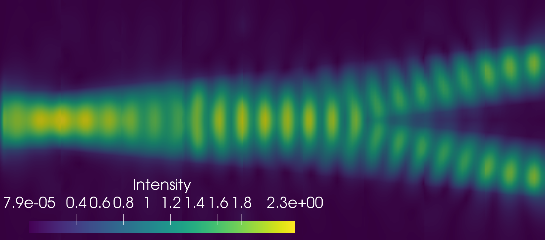
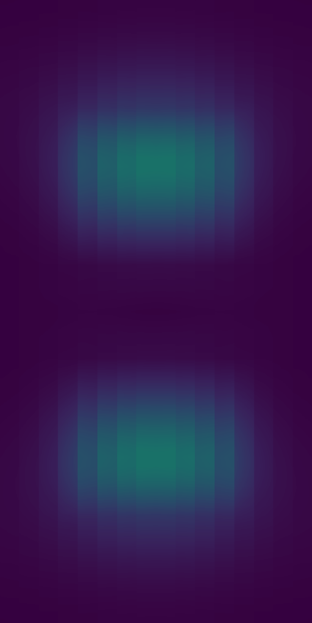
Figure 3: Intensity plot of the y beam splitter, on the left side is the intensity on the x-y plane and on the right side is the intensity at the output.

5 Conclusion

In this contribution, we implemented a domain decomposition method with a block preconditioner for the time harmonic Maxwell equations. Therein, a crucial aspect is the construction of the subdomain interface conditions. Our algorithmic developments are demonstrated for two configurations of practical relevance, namely a block benchmark and a Y beam splitter.

- [1] P. R. Amestoy, A. Buttari, J.-Y. L’Excellent, and T. Mary. Performance and scalability of the block low-rank multifrontal factorization on multicore architectures. ACM Trans. Math. Software, 45(1):Art. 2, 26, 2019.
- [2] D. Arndt, W. Bangerth, B. Blais, and et al. The deal.II library, Version 9.2. J. Numer. Math., 28(3):131–146, 2020.
- [3] L. Berger-Vergiat, C. A. Glusa, J. J. Hu, M. Mayr, A. Prokopenko, C. M. Siefert, R. S. Tuminaro, and T. A. Wiesner. MueLu multigrid framework. http://trilinos.org/packages/muelu, 2019.
- [4] M. Bonazzoli, V. Dolean, I. G. Graham, E. A. Spence, and P.-H. Tournier. Domain decomposition preconditioning for the high-frequency time-harmonic Maxwell equations with absorption. Math. Comp., 88(320):2559–2604, 2019.
- [5] M. E. Bouajaj, B. Thierry, X. Antoine, and C. Geuzaine. A quasi-optimal domain decomposition algorithm for the time-harmonic maxwell’s equations. Journal of Computational Physics, 2015.
- [6] M. Bürg. Convergence of an automatic hp-adaptive finite element strategy for maxwell’s equations. Applied Numerical Mathematics, 72:188–204, 10 2013.
- [7] V. Dolean, M. J. Gander, and L. Gerardo-Giorda. Optimized Schwarz methods for Maxwell’s equations. SIAM J. Sci. Comput., 31(3):2193–2213, 2009.
- [8] O. G. Ernst and M. J. Gander. Why it is difficult to solve Helmholtz problems with classical iterative methods. 83:325–363, 2012.
- [9] V. Girault and P.-A. Raviart. Finite element methods for Navier-Stokes equations, volume 5 of Springer Series in Computational Mathematics. Springer-Verlag, Berlin, 1986. Theory and algorithms.
- [10] I. G. Graham, E. A. Spence, and E. Vainikko. Domain decomposition preconditioning for high-frequency Helmholtz problems with absorption. Math. Comp., 86(307):2089–2127, 2017.
- [11] A. Grayver and T. Kolev. Large-scale 3d geoelectromagnetic modeling using parallel adaptive high-order finite element method. GEOPHYSICS, 80:E277–E291, 11 2015.
- [12] G. Haase, M. Kuhn, U. Langer, S. Reitzinger, and J. Schöberl. Parallel Maxwell Solvers, pages 71–78. Lecture Notes in Computational Science and Engineering, Vol. 18. Springer, Germany, 2001.
- [13] M. A. Heroux, R. A. Bartlett, V. E. Howle, R. J. Hoekstra, J. J. Hu, T. G. Kolda, R. B. Lehoucq, K. R. Long, R. P. Pawlowski, E. T. Phipps, A. G. Salinger, H. K. Thornquist, R. S. Tuminaro, J. M. Willenbring, A. Williams, and K. S. Stanley. An overview of the trilinos project. ACM Trans. Math. Softw., 31(3):397–423, 2005.
- [14] U. Langer, D. Pauly, and S. Repin, editors. Maxwell’s Equations. volume 24 of Radon Series on Computational and Applied Mathematics, Berlin. de Gruyter, 2019.
- [15] P. Monk. Finite Element Methods for Maxwell’s Equations. Oxford Science Publications, 2003.
- [16] A. Toselli and O. Widlund. Domain decomposition methods - algorithms and theory. Volume 34 of Springer Series in Computational Mathematics. Springer, Berlin, Heidelberg, 2005.
- [17] S. Zaglmayr. High Order Finite Element Methods for Electromagnetic Field Computation. PhD thesis, Johannes Kepler University Linz, 2006.