Quantifying Uncertainty in Deep Spatiotemporal Forecasting

Abstract.

Deep learning is gaining increasing popularity for spatiotemporal forecasting. However, prior works have mostly focused on point estimates without quantifying the uncertainty of the predictions. In high stakes domains, being able to generate probabilistic forecasts with confidence intervals is critical to risk assessment and decision making. Hence, a systematic study of uncertainty quantification (UQ) methods for spatiotemporal forecasting is missing in the community. In this paper, we describe two types of spatiotemporal forecasting problems: regular grid-based and graph-based. Then we analyze UQ methods from both the Bayesian and the frequentist point of view, casting in a unified framework via statistical decision theory. Through extensive experiments on real-world road network traffic, epidemics, and air quality forecasting tasks, we reveal the statistical and computational trade-offs for different UQ methods: Bayesian methods are typically more robust in mean prediction, while confidence levels obtained from frequentist methods provide more extensive coverage over data variations. Computationally, quantile regression type methods are cheaper for a single confidence interval but require re-training for different intervals. Sampling based methods generate samples that can form multiple confidence intervals, albeit at a higher computational cost.

1. Introduction

Forecasting the spatiotemporal evolution of time series data is at the core of data science. Spatiotemporal forecasting exploits the spatial correlations to improve the forecasting performance for multivariate time series (Cressie and Wikle, 2015). Many works have used deep learning for spatiotemporal forecasting, applied to various domains from weather (Xingjian et al., 2015; Yi et al., 2018) to traffic (Li et al., 2018; Geng et al., 2019) forecasting. However, the majority of existing works focus on point estimates without generating confidence intervals. The resulting predictions fail to provide credibility for assessing potential risks and assisting decision making, which is critical especially in high-stake domains such as public health and transportation.

It is known that deep neural networks are poor at providing uncertainty and tend to produce overconfident predictions (Amodei et al., 2016). Therefore, uncertainty quantification (UQ) is receiving growing interests in deep learning (Gal and Ghahramani, 2016; Vandal et al., 2018; Qiu et al., 2019; Wen et al., 2017). There are roughly two types of UQ methods in deep learning. One leverages frequentist thinking and focuses on robustness. Perturbations are made to the inference procedure in initialization  (Lakshminarayanan et al., 2017; Fort et al., 2019), neural network weights (Gal and Ghahramani, 2016), and datasets (Lee et al., 2015; Osband et al., 2016). The other type is Bayesian, which aims to model posterior beliefs of network parameters given the data (Neal, 2012; Kingma and Welling, 2013; Heek and Kalchbrenner, 2019). A common focal point of both approaches is the generalization ability of the neural networks. In forecasting, we not only wish to explain in-distribution examples, but also generalize to future data with model misspecifications and distribution shifts. Time series data provide the natural laboratory for studying this problem.

Spatiotemporal sequence data pose unique challenges to UQ: (1) Spatiotemporal dependency: accurate forecasts require models that can capture both spatial and temporal dependencies. (2) Evaluation metrics: point estimates often use mean squared error (MSE) as a metric, which only measures the averaged point-wise error for the sequence. For uncertainty, common metrics such as held-out log-likelihood require exact likelihood computation. The number of possibilities grows exponentially with the length of the sequence. (3) Forecasting horizon: the sequential dependency in time series often leads to error propagation for long-term forecasting, so does uncertainty. Unfortunately, most existing deep UQ methods deal with scalar classification/regression problems with a few exceptions. (Vandal et al., 2018) proposes to use concrete dropout for climate down-scaling but not for forecasting. (Wang et al., 2019) proposes a Bayesian neural network based on variational inference. Still, a systematic study of UQ methods for spatiotemporal forecasting with deep learning is missing in the data science community.

In this paper, we conduct a benchmark study of deep uncertainty quantification for spatiotemporal forecasting. We investigate spatiotemporal forecasting problems on a regular grid as well as on a graph. We compare 2 types of UQ methods: frequentist methods including Bootstrap, Quantile regression, Spline Quantile regression and Mean Interval Score regression; and Bayesian methods including Monte Carlo dropout, and Stochastic Gradient Markov chain Monte Carlo (SG-MCMC). We analyze the properties of both frequentist and Bayesian UQ methods, as well as their practical performances. We further provide a recipe for practitioners when tackling UQ problems in deep spatiotemporal forecasting. We experimented with many real-world forecasting tasks to validate our hypothesis: road network traffic forecasting, epidemic forecasting, and air quality prediction.

Our contributions include:

• We conduct the first systematic benchmark study for deep learning uncertainty quantification (UQ) in the context of multi-step spatiotemporal forecasting.

• We cast frequentist and Bayesian UQ methods under a unified framework and adapt 6 UQ methods for grid-based and graph-based spatiotemporal forecasting problems.

• Our study reveals that posterior sampling excels at mean prediction whereas quantile and mean interval score regression obtain confidence levels that cover data variations better.

• We also notice that the sample complexity of posterior sampling is lower than that of the bootstrapping method, potentially due to posterior contraction (Wilson and Izmailov, 2020).

2. Related Work

2.1. Spatiotemporal Forecasting

Spatiotemporal forecasting is challenging due to the higher-order dependencies in space, time, and variables. Classic Bayesian statistical models (Cressie and Wikle, 2015) often require strong modeling assumptions. There is a growing literature on using deep learning due to its flexibility. Depending on the geometry of the space, the existing methods fall into two categories: regular grid-based such as Convolutional LSTM (Xingjian et al., 2015; Lin et al., 2020; Wang et al., 2017; Yao et al., 2018; Yao et al., 2019) and graph-based such as Graph Convolutional LSTM (Yu et al., 2018; Geng et al., 2019; Li et al., 2018). The high-level idea behind these architectures is to integrate spatial embedding using (Graph) Convolutional neural networks with deep sequence models such as LSTM. However, most existing works in deep learning forecasting only produce point estimation rather than probabilistic forecasts with built-in uncertainty.

2.2. Uncertainty Quantification

Two types of deep UQ methods prevail in data science. Bayesian methods model the posterior beliefs of network parameters given the data. For example, Bayesian neural networks learning (BNN) uses approximate Bayesian inference to improve inference efficiency. Wang et al. (2016) proposes natural parameter network using exponential family distributions. Shekhovtsov and Flach (2018) proposes new approximations for categorical transformations. However, these BNNs are focused on classification problems rather than forecasting. (Vandal et al., 2018) use concrete dropout for climate downscaling. (Wang et al., 2019) proposes a Bayesian deep learning model VI for weather forecasting. On the other hand, frequentist UQ methods emphasize the robustness against variations in the data. For instance, (Pearce et al., 2018; Gasthaus et al., 2019) propose prediction intervals as the forecasting objective. (Alaa and van der Schaar, 2020) proposed a UQ method with bootstrapping using the influence function. This paper extends previous works and studies the efficacy and efficiency of various methods for UQ in spatiotemporal forecasts. We defer the detailed discussion of these methods to Section 4.3. To the best of our knowledge, there does not exist a systematic benchmark study of these UQ methods for deep spatiotemporal forecasting.

3. Deep Spatiotemporal Forecasting

3.1. Problem Definition

Given multivariate time series $\mathcal{X}=({\mathbf{X}}_{1},\cdots,{\mathbf{X}}_{t})$ of $t$ time step, where ${\mathbf{X}}_{t}\in\mathbb{R}^{P\times D}$ indicating $D$ features from $P$ locations. We also have a spatial correlation matrix ${A}\in\mathbb{R}^{P\times P}$ indicating the spatial proximity. Deep spatiotemporal forecasting approximates a function $f$ with deep neural networks such that:

(1) $$f:(\mathcal{X};{A})\rightarrow({\mathbf{X}}_{t+1},\cdots,{\mathbf{X}}_{t+H};{A})$$

where $H$ is the forecasting horizon.

Spatiotemporal forecasting exploits spatial correlations to improve the prediction performance. A popular idea behind existing deep learning models is to integrate a spatial embedding of ${\mathbf{X}}_{t}$ into a deep sequence model such as an RNN or LSTM. Mathematically speaking, that means to replace the matrix multiplication operator in an RNN with a convolution or graph convolution operator.

For grid-based data we can use convolution, which is the key idea behind ConvLSTM (Xingjian et al., 2015). As the locations are distributed as a grid, we reshape ${\mathbf{X}}_{t}$ into a tensor of shape $W\times H\times D$ with $W\times H=P$ representing the width and the height of the grid. A convolutional RNN model becomes:

(2) $${\mathbf{h}}_{t+1}=\sigma(W^{h}\cdot{\mathbf{h}}_{t}+W^{x}\cdot{\mathbf{X}}_{t})\longrightarrow{\mathbf{h}}_{t+1}=\sigma(W^{h}\ast{\mathbf{h}}_{t}+W^{x}\ast{\mathbf{X}}_{t})$$

where ${\mathbf{h}}_{t}$ are the hidden states of the RNN and $\ast$ is the convolution $(W\ast{\mathbf{X}})[m,n]=\sum_{i}\sum_{j}W[i,j]{\mathbf{X}}_{t}[m-i,n-j]$.

For graph-based data we use graph convolution, leading to graph convolutional RNN, similar to the design of DCRNN (Li et al., 2018):

(3) $${\mathbf{h}}_{t+1}=\sigma(W\ast_{g}{\mathbf{h}}_{t}+W\ast_{g}{\mathbf{X}}_{t})$$

Where $\ast_{g}$ stands for graph convolution. There are many variations for graph convolution or graph embedding. One example is

(4) $$W\ast_{g}{\mathbf{X}}_{t}=W\cdot(D^{-1}A)\cdot{\mathbf{X}}_{t}$$

Here $D\in\mathbb{R}^{P\times P}$ contains the diagonal element of $A$. One can also replace the random walk matrix $D^{-1}A$ with the normalized Laplacian matrix $I-D^{1/2}(D-A)D^{1/2}$ as in (Kipf and Welling, 2016).

These deep learning models are developed only for point estimation. We will use them as base models to design and compare various deep UQ methods for probabilistic forecasts.

3.2. Evaluation Metrics

For point estimation, mean squared error (MSE) or mean absolute error (MAE) are well-established metrics. But for probabilistic forecasts, MSE is insufficient as it cannot characterize the quality of the prediction confidence. While held-out likelihood is the gold standard in the existing UQ literature, it is difficult to use for deep learning as they often do not generate explicit likelihood outputs (Kingma and Dhariwal, 2018). Instead, we revisit a key concept from statistics and econometric called Mean Interval Score (Gneiting and Raftery, 2007).

Mean Interval Score (MIS) is a scoring function for interval forecasts. It is also known as Winkler loss (Askanazi et al., 2018). It rewards narrower confidence or credible intervals and encourages intervals that include the observations (coverage). From a computational perspective, MIS is preferred over other scoring functions such as the Brier score (Brier, 1950), Continuous Ranked Probability Score (CRPS) (Matheson and Winkler, 1976; Hamill and Wilks, 1995; Gneiting and Raftery, 2007) as it is intuitive and easy to compute. MIS only requires three quantiles while CRPS requires integration over all quantiles. From a statistical perspective, MIS does not constrain the model to be parametric, nor does it require explicit likelihood functions. It is therefore better suited for comparison across a wide range of methods.

We formally define MIS for estimated upper and lower confidence bounds. For a one-dimensional random variable $Z\sim\mathbb{P}_{Z}$, if the estimated upper and lower confidence bounds are $u$ and $l$, where $u$ and $l$ are the $(1-\frac{\rho}{2})$ and $\frac{\rho}{2}$ quantiles for the $(1-\rho)$ confidence interval, MIS is defined using samples $z_{i}\sim\mathbb{P}_{Z}$:

$$\mathrm{MIS}_{N}(u,l;\rho)=\frac{1}{N}\sum_{i=1}^{N}\Big{\{}\left(u-l\right) +\frac{2}{\rho}(z_{i}-u){\mathds{1}\left\{z_{i}>u\right\}}$$

$$+\frac{2}{\rho}(l-z_{i}){\mathds{1}\left\{z_{i}<l\right\}}\Big{\}}.$$

In the large sample limit, MIS converges to the following expectation:

$$\textstyle\mathrm{MIS}_{\infty}(u,l;\rho)=(u-l)+\frac{2}{\rho}\left(\mathbb{E}\left[Z-u|Z>u\right]+\mathbb{E}\left[l-Z|Z<l\right]\right).$$

We prove in the following two novel propositions about the consistency of MIS as a scoring function, which demonstrates that minimizing MIS will lead to unbiased estimates for the confidence intervals. The first proposition is concerned with the consistency of MIS in the large sample limit and the second studies the finite sample consistency of it. Proofs for both propositions are deferred to Appendix A.

Proposition 0.

Assume that the distribution $\mathbb{P}_{Z}$ of $Z$ has a probability density function. Then for $(u^{*},l^{*})=\operatorname*{argmin}_{u>l;u,l\in\real}\mathrm{MIS}_{\infty}(u,l;\rho)$, $[l^{*},u^{*}]$ is the $(1-\rho)$ confidence level.

Proposition 0.

For $(u^{*},l^{*})=\arg\min_{u>l;u,l\in\real}\mathrm{MIS}_{N}(u,l;\rho)$, $[l^{*},u^{*}]$ is the $(1-\rho)$ quantile of the empirical distribution formed by the samples $\{z_{1},\cdots,z_{N}\}$.

Note from Proposition 2 that the optimal interval for $\mathrm{MIS}_{N}$ contains $\rho$ portion of the data points, because of the balance it strikes between the reward towards narrower intervals and the penalty towards excluding observations. Next, we describe a unified framework based on statistical decision theory to better understand uncertainty quantification.

4. Uncertainty Quantification in Spatiotemporal Forecasts

We cast uncertainty quantification from frequentist and Bayesian perspectives into a single framework. Then we describe both the Bayesian and frequentist techniques to enable deep spatiotemporal forecasting models to generate probabilistic forecasts.

4.1. A Unified Framework

We start from a statistical decision theory point of view to examine uncertainty quantification. Assume that each datum $\mathcal{X}$ and its label $\mathcal{Y}$ are generated from a mechanism specified by a probability distribution with parameter $\theta$: $p(\mathcal{Y}|\mathcal{X};\theta)$. We further assume that the parameter $\theta$ is distributed according to $p(\theta)$. The goal of a probabilistic inference procedure is to minimize the statistical risk, which is an expectation of the loss function over the distribution of the data as well as $p(\theta)$, the distribution of the class of models considered. Concretely, consider an estimator $\hat{\theta}$ of $\theta$, which is a measurable function of the dataset $\{\mathcal{X}\}=\{\mathcal{X}_{0},\cdots,\mathcal{X}_{N}\}$. We wish to minimize its risk:

(5) $$\textstyle{\rm Risk}(\hat{\theta},\theta) = \mathbb{E}\left[\|f(\hat{\theta})-f(\theta)\|^{2}\right]$$

$$= \mathbb{E}_{\theta}\left[\mathbb{E}\left[\|f(\hat{\theta})-f(\theta)\|^{2}\Big{|}\theta\right]\right]$$

(6) $$= \mathbb{E}\left[\mathbb{E}_{\theta}\left[\|f(\hat{\theta})-f(\theta)\|^{2}\Big{|}\{\mathcal{X}\}\right]\right],$$

where in this paper, function $f$ is taken to be the prediction of the deep learning model given its parameters.

When we design an inferential procedure, we can use equation 5 or equation 6. If we take the procedure of equation 5 and be a frequentist, we first seek the estimator $\hat{\theta}$ to minimize $\mathbb{E}[\|f(\hat{\theta})-f(\theta)\|^{2}|\theta]$. In practice, we minimize the empirical risk over the training dataset $\{\mathcal{X}\}$, $\frac{1}{N}\sum_{i\in\{0,\cdots,N\}}(f(\mathcal{X}_{i};\hat{\theta})-\mathcal{Y}_{i})^{2}$, instead of the original expectation that is agnostic to the algorithms.

If we take the procedure of equation 6 and be Bayesian, we first take the expectation over the distribution of the parameter space $\theta$, conditioning on the training dataset $\{\mathcal{X}\}$. We can find that minimizing $\mathbb{E}_{\theta}\left[\|f(\hat{\theta})-f(\theta)\|^{2}\Big{|}\{\mathcal{X}\}\right]$ is equivalent to taking $f(\hat{\theta})$ to be $\mathbb{E}_{\theta}\left[f(\theta)\right]$. For a proper prior distribution over $\theta$, this boils down to the posterior mean of $f(\theta)$. In this work, we also take function $f$ to be the output of the model.

To quantify uncertainty of the respective approaches, it is important to capture variations in $\theta$ that determine the distribution of the data. There are two sources of in-distribution uncertainties corresponding to different modes of variations in $\theta$: effective dimension of the estimator $\hat{\theta}$ being smaller than that of the true $\theta$, oftentimes addressed to as the bias correction problem; and the variance of the estimator $\hat{\theta}$, often approached via parameter calibration. On top of that, we are also faced with distribution shift that poses additional challenges.

Frequentist methods aim to directly capture variations in the data. For example, quantile regression explores the space of predictions within the model class by ensuring proper coverage of the data set. bootstrap method resamples the data set to target both the bias correction and parameter calibration problems, albeit possessing a potentially high resampling variance. Bayesian methods often leverage prior knowledge about the distribution of $\theta$ and use MCMC sampling to integrate different models to capture both variations in the parameter space.

In practice, it is important to understand the sample complexity (e.g., number of resampling runs in bootstrap or number of MCMC samples) of all methods and how it scales with the model and data complexity. For deep learning models, it is also crucial to capture the trade-off between the variance incurred by the algorithms and their computation complexity. To understand the performance of the uncertainty quantification methods, we apply the statistically consistent metric MIS to measure how well the confidence intervals computed from either frequentist or Bayesian methods capture the uncertainty of the predictions given the data. In what follows, we introduce the computation methods for uncertainty quantification.

4.2. Frequentist UQ Methods

We start by describing the frequentist methods. The general idea behind them is to directly capture variations in the dataset, either by resampling the data or by learning an interval bound to encompass the dataset.

Bootstrap. The (generalized) bootstrap method (Efron and Hastie, 2016) randomly generates in each round a weight vector over the index set of the data. The data are then resampled according to the weight vector. With every resampled dataset, we retrain our model and generate predictions. Using the predictions from different retrained models, we infer the $(1-\rho)$ confidence interval from the $(1-\frac{\rho}{2})$ and $\frac{\rho}{2}$ quantiles based on Proposition 2. The quantiles can be estimated using the order statistics of Monte Carlo samples.

MIS Regression For a fixed confidence level $\rho$, we can directly minimize MIS to obtain estimates of the confidence intervals. Specifically, we use MIS as a loss function for deep neural networks, we use a multi-headed model to jointly output the upper bound $u(x)$, lower bound $l(x)$, and the prediction $f(x)$ for a given input $x$, and minimize the neural network parameter $\theta$:

$$L_{\text{MIS}}(y,u(x),l(x),f(x);\theta,\rho)$$

$$=\min\limits_{\theta}\Big{\{}\textstyle\mathbb{E}_{(x,y)\sim\mathcal{D}}[(u(x)-l(x))+\frac{2}{\rho}(y-u(x)){\mathds{1}\left\{y>u(x)\right\}}$$

(7) $$\;\quad\qquad\textstyle+\frac{2}{\rho}(l(x)-y){\mathds{1}\left\{y<l(x)\right\}}+|y-f(x)|]\Big{\}}$$

Here ${\mathds{1}\left\{\cdot\right\}}$ is an indicator function, which can be implemented using the identity operator over the larger element in Pytorch.

Quantile Regression We can use the one-sided quantile loss function  (Koenker, 2005) to generate predictions for a fixed confidence level $\rho$. Given an input $x$, and the output $f(x)$ of a neural network, parameterized by $\theta$, quantile loss is defined as follows:

$$L_{\text{Quantile}}(y,f(x);\theta,\rho)$$

(8) $$=\min\limits_{\theta}\Big{\{}\mathbb{E}_{(x,y)\sim\mathcal{D}}[(y-f(x))(\rho-{\mathds{1}\left\{y<f(x)\right\}}]\Big{\}}$$

Quantile regression behaves similarly as the MIS regression method. Both methods generate one confidence interval per time. Similar ideas of directly optimizing the prediction interval using different variations of quantile loss have also been explored by Kivaranovic et al. (2020); Tagasovska and Lopez-Paz (2019); Pearce et al. (2018).

One caveat of these methods is that different predicted quantiles can cross each other due to variations given finite data. This will lead to a strange phenomenon when the size of the data set and the model capacity is limited: the higher confidence interval does not contain the interval of lower confidence level or even the point estimate. One remedy for this issue is to add variations in both the data and the parameters to increase the effective data size and model capacity. In particular, during training, we can use different subsets of data and repeat the random initialization from a prior distribution to form an ensemble of models. In this way, our modified MIS and quantile regression methods have integrated across different models to quantify the prediction uncertainty and have taken advantage of the Bayesian philosophy.

Another solution to alleviate the quantile crossing issue is to minimize CRPS by assuming the quantile function to be a piecewise linear spline with monotonicity (Gasthaus et al., 2019), a method we call Spline Quantile regression (SQ). In the experiment, we also included this method for comparison.

4.3. Bayesian UQ Methods

We describe the Bayesian approaches to UQ. These methods impose a prior distribution over the class of models and average across them, either via MCMC sampling or variational approximations.

Stochastic Gradient MCMC (SG-MCMC) To estimate expectations or quantiles according to the posterior distribution over the parameter space, we use SG-MCMC (Welling and Teh, 2011; Ma et al., 2015). We find in practice that the stochastic gradient thermostat method (SGNHT) (Ding et al., 2014; Shang et al., 2015) is particularly useful in controlling the stochastic gradient noise. This is consistent with the observation in (Heek and Kalchbrenner, 2019) where stochastic gradient thermostat method is applied to an i.i.d. image classification task.

To generate samples of model parameters $\theta$ (with a slight abuse of notation) according to SGNHT, we first denote the loss function (or the negative log-likelihood) over a minibatch of data as $\widetilde{\mathcal{L}}(\theta)$. We then introduce hyper-parameters including the diffusion coefficients $A$ and the learning rate $h$ and make use of auxiliary variables $p\in{}^{d}$ and $\xi\in\real$ in the algorithm. We randomly initialize $\theta$, $p$, and $\xi$ and update according to the following update rule.

(12) $$\left\{\begin{array}[]{l}\theta_{k+1}=\theta_{k}+p_{k}h\\ p_{k+1}=p_{k}-\nabla\widetilde{\mathcal{L}}(\theta)h-\xi_{k}p_{k}h+\mathcal{N}(0,2Ah)\\ \xi_{k+1}=\xi_{k}+\left(\frac{p_{k}^{\rm T}p_{k}}{d}-1\right)h.\end{array}\right.$$

Upon convergence of the above algorithm at $K$-th step, $\theta_{K}$ follows the distribution of the posterior. We run parallel chains to generate different samples according to the posterior and quantify the prediction uncertainty.

Approximate Bayesian Inference SG-MCMC can be computationally expensive. There are also approximate Bayesian inference methods introduced to accelerate the inference procedures (Maddox et al., 2019; Dusenberry et al., 2020). In particular, the Monte Carlo (MC) drop-out method sets some of the network weights to zero according to a prior distribution (Gal et al., 2017). This method serves as a simple alternative to variational Bayes methods which approximate the posterior (Blundell et al., 2015; Graves, 2011; Louizos and Welling, 2016; Rezende et al., 2014; Qiu et al., 2019). We use the popular MC dropout (Gal et al., 2017) method in the experiments.

4.4. A Recipe for UQ in Practice

The above-mentioned UQ methods have different properties. Table 1 shows an overall comparison of different UQ methods for deep spatiotemporal forecasting. The relative computation budget is displayed in the “Computation” row. The numbers represent the numbers of parallel cores required to finish computation within the same amount of time.

Method	Bootstrap	Quantile	SQ	MIS	MC Dropout	SG-MCMC
Computation	25	1	1	1	1	25
Small sample	$\times$	$\times$	$\times$	$\times$	$\times$	✓
Consistency	✓	$\times$	$\times$	$\times$	$\times$	✓
Accuracy	✓	✓	✓	✓	✓	✓✓
Uncertainty	$\times$	✓	$\times$	✓✓	$\times$	✓

Table 1. Comparison of different deep uncertainty quantification methods for forecasting. Double check marks represent robustly highest performance in experiments.

It is worth noting that when comparing computational budgets, we assume only one level of confidence (usually $95\%$) is estimated. If $n$ confidence levels are required, then the computation complexity of quantile regression and MIS regression multiplies by $n$, whereas the computational budgets for the rest of the methods remain unchanged. Through our experiments, we provide the following recipe for practitioners.

• Large data, sufficient computation: We recommend SG-MCMC and bootstrap as both methods generate accurate predictions, high-quality uncertainty quantification, which means the corresponding MIS is small, and have asymptotic consistency.

• Large data, limited computation: We recommend MIS and quantile regression. Both of them prevail in providing accurate results with high-quality uncertainty quantification.

• Small data: Bayesian learning with SG-MCMC can have an advantage here. By choosing a proper prior, SG-MCMC can lead to better generalization. Frequentist methods are often inferior with very limited samples, especially for mean prediction, see experiments for more details.

• Asymptotic consistency: Both bootstrap and SG-MCMC methods are asymptotically consistent, making them the default choice when the computational budget and the dataset are sufficient. When the computational budget is restrictive, the comparison is about sample complexity: the number of bootstrap resampling versus the number of MCMC chains determines which method needs more parallel computing resources. We found in our experiments that the sample complexity of bootstrap is consistently higher than that of posterior sampling.

5. Experiments

We benchmark the performance of both frequentist and Bayesian UQ methods on many spatiotemporal forecasting applications, including air quality PM2.5, road network traffic, and COVID-19 incident deaths. Air quality PM2.5 is on a regular grid, while traffic and COVID-19 are on graphs.

5.1. Datasets

Air Quality PM 2.5

The air quality PM 2.5 dataset contains hourly weather and air quality data in Beijing provided by the KDD competition of 2018 . The weather data is at the grid level ($21\times 31$), which contains temperature, pressure, humidity, wind direction, and wind speed, forming a $21\times 31\times 5$ tensor at each timestamp. The air quality data is from 35 stations in Beijing. The air quality index we considered is PM2.5 measured in micrograms per cubic meter of air ($\mu g/m^{3}$). According to the air quality index provided by the U.S. Environmental Protection Agency (US-EPA, 2012), the air quality is unhealthy from 101 to 300, and hazardous from 301 to 500. We follow the setting in (Liu and Shuo, 2018) to map PM2.5 to grid-based data using the weighted average over stations:

(13) $$PM2.5_{k}=\frac{1}{\sum_{i}{\frac{1}{d_{i,k}^{2}+\epsilon}PM2.5_{i}}}$$

Here $d_{1,cell}$ is the distance between station i and the grid cell k. $\epsilon$ is introduced to prevent divide-by-zero error.

METR-LA Road Network Traffic

The METR-LA (Jagadish et al., 2014) dataset contains $4$ months vehicle speed information from loop detector sensors in Los Angeles County highway system. The maximum speed limit on most California highways is 65 miles per hour. The task is to forecast the traffic speed for $207$ sensors simultaneously. We build the spatial correlation matrix $A$ using road network distances between sensors $v_{i}$ and $v_{j}$ and a Gaussian kernel:

$$A_{ij}=\exp\Big{(}-\frac{d(v_{i},v_{j})}{\sigma^{2}}\Big{)}$$

COVID-19 Incident Death

The COVID-19 dataset contains reported deaths from Johns Hopkins University (Dong et al., 2020) and the death predictions from a mechanistic, stochastic, and spatial metapopulation epidemic model called Global Epidemic and Mobility Model (GLEAM) (Balcan et al., 2009, 2010; Tizzoni et al., 2012; Zhang et al., 2017b; Chinazzi et al., 2020; Davis et al., 2020). Both data are recorded for the $50$ US states during the period from May 24th to Sep 12th, 2020. We use the residual between the reported death and the corresponding GLEAM predictions to train the model (http://covid19.gleamproject.org/).

We construct the spatial correlation matrix $A$ using air traffic between different states. Each element in the matrix is the average number of passengers traveling between two states daily. The air traffic data were obtained from the Official Aviation Guide (OAG) and the International Air Transportation Association (IATA) databases (updated in $2021$) (OAG, Aviation Worlwide Limited, 2021; IATA, International Air Transport Association, 2021). See Appendix B.2 for details.

5.2. Experiment Setup

For all experiments, we start with a deep learning point estimate model (Point) based on Sec. 3.1. We use as deep learning models ConvLSTM (Xingjian et al., 2015) for grid-based data and DCRNN (Li et al., 2018) for graph-based data. Then we modify and adapt the deep learning models to incorporate 6 different UQ methods as in Sec.4.

For the ConvLSTM model (Xingjian et al., 2015), we follow the best setting reported in (Liu and Shuo, 2018) with $3\times 3$ filter, 256 hidden states, and 2 layers. We applied early stopping, autoregressive learning, and gradient clipping (Zhang et al., 2019) to improve the generalization. As PM2.5 is closely related to weather, we use a combined loss

$$\mathcal{L}=MAE(weather)\times 0.2+MAE(PM2.5)$$

For the DCRNN model, we use the exact setting in (Li et al., 2018) for the traffic dataset and use calibrated network distance to construct the graph. We applied early stopping, curriculum learning, and gradient clipping (Zhang et al., 2019) to improve the generalization. For the COVID-19 dataset, we chose to forecast the residual rather than directly predicting the death number because the latter has lower accuracy due to limited samples, see Sec. 6.2 for quantitative comparisons.

We report the mean absolute error (MAE) as a point estimate metric. For UQ metric, we use MIS suggested in Sec 3.2 for 95% confidence intervals. As MIS combines both the interval and coverage, we also report the interval score, which is the average difference between the upper and lower bounds.

Horizon H	Metric	Point	Bootstrap (F)	Quantile (F)	SQ (F)	MIS(F)	MC Dropout (B)	SG-MCMC (B)
Air Quality PM 2.5
first 12 hrs	MAE	22.93	22.27	24.89	23.35	24.41	22.11	21.83
	MIS	—	469.36	157.53	188.30	147.68	736.50	223.63
	Interval width	—	28.80	115.25	82.45	137.34	8.47	57.44
first 24 hrs	MAE	25.17	23.37	26.25	24.67	25.93	24.42	23.10
	MIS	—	515.51	171.12	217.34	156.02	828.42	279.21
	Interval width	—	35.35	121.51	84.39	141.74	8.46	56.22
total 48 hrs	MAE	26.77	25.69	27.82	26.47	30.20	26.03	24.73
	MIS	—	531.19	189.35	253.15	179.96	881.05	315.34
	Interval width	—	31.43	130.17	90.09	151.61	9.16	55.66
METR-LA Traffic
15 min	MAE	2.38	2.63	2.43	2.67	2.63	2.47	2.32
	MIS	—	39.76	18.32	29.04	18.26	27.61	32.21
	Interval width	—	5.80	12.42	8.38	12.46	8.99	8.73
30 min	MAE	2.73	3.19	2.79	3.10	3.08	2.94	2.54
	MIS	—	38.48	21.54	40.93	21.09	33.38	31.87
	Interval width	—	7.86	13.48	8.37	13.99	11.10	12.62
1 hour	MAE	3.14	3.99	3.19	3.75	3.65	3.70	3.00
	MIS	—	38.58	25.74	60.56	24.33	43.11	30.35
	Interval width	—	11.65	14.50	8.38	15.55	14.46	18.79
COVID-19 Incident Death
1W	MAE	34.32	32.57	36.63	34.42	39.03	34.27	29.72
	MIS	—	856.87	413.37	1049.69	427.53	790.24	563.77
	Interval width	—	32.48	190.98	23.73	227.19	47.79	47.05
2W	MAE	33.72	32.38	36.81	34.03	36.35	33.64	27.65
	MIS	—	762.55	363.14	1010.97	379.27	686.43	599.14
	Interval width	—	36.25	219.06	24.46	260.24	55.93	45.45
3W	MAE	41.37	40.33	44.29	41.24	43.15	41.26	34.62
	MIS	—	1028.63	411.05	1292.98	402.46	905.66	821.71
	Interval width	—	39.95	242.47	24.16	291.96	62.39	46.16
4W	MAE	42.37	41.71	46.20	41.79	44.45	42.28	40.66
	MIS	—	1035.26	455.27	1303.02	428.82	891.45	852.26
	Interval width	—	43.61	262.09	23.85	316.13	67.52	47.58

Table 2. Performance comparison of 6 different UQ methods applied to grid-based air quality PM2.5, graph-based traffic and COVID-19 incident death forecasting. (F) indicates frequentist methods and (B) standards for Bayesian methods. We compare these methods using the mean absolute error (MAE), the mean interval score (MIS), and the width of the confidence bounds.

5.3. Implementation Details

We adapt ConvLSTM and DCRNN to implement various UQ methods with the following parameter settings.

Bootstrap We randomly dropped 50$\%$ of training data while keeping the original validation and testing data. We obtain 25 samples for constructing mean prediction and confidence intervals.

Quantile regression We apply the pinball loss function (Koenker, 2005) with the corresponding quantile (0.025, 0.5, 0.975). The model and learning rate setup is the same as point estimation.

SQ regression We use the linear spline quantile function to approximate a quantile function and use the CRPS as the loss function. For every point prediction, there are 11 trained parameters to construct the quantile function. The 1^st parameter is the intercept term. The next 5 can be transformed to the slopes of 5 line segments. The last 5 can be transformed to a vector of the 5 knots’ positions. The model and learning rate setup is the same as point estimation.

MIS regression We combine MAE with MIS (equation 7) and directly minimize this loss function. The model and learning rate setup is the same as (Li et al., 2018).

MC Dropout We implement the algorithm provided by (Zhu and Laptev, 2017) and simplify the model by only considering the model uncertainty. We apply random dropout through the testing process with 5% drop rate and iterate 50 times to achieve a stable prediction. The result for comparison averages the performance of 10 trails.

SG-MCMC We set the learning rate of SG-MCMC $h=5e^{-4}$, as defined in Eqn. 12, and we selected a Gaussian prior $\theta\sim\mathcal{N}(0,4.0)$ with random initialization as $\theta_{0}\sim\mathcal{N}(0,0.2)$. We selected different priors and initialization parameters around the choices above. The performances are fairly stable for different choices as long as the model would not diverge (e.g., random initialization variance too large). We note here a symmetric Gamma prior could also work in this case with $\theta\sim\Gamma(0.1,1)$. We apply early stopping at epoch 50, and it helps to improve the generalization on testing set. Our result is averaged from 25 posterior samples.

We use V100 GPUs to perform all the experiments. In addition to the MAE and MIS scores discussed in section 3.2, we also include the widths of the confidence bounds to demonstrate the coverage.

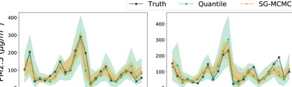
Figure 1. 12 hours ahead (Left) and 24 hours ahead (Right) Air quality PM 2.5 forecasting over 24 day time span on a randomly selected grid cell.

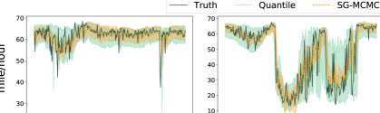
Figure 2. 15 min ahead traffic forecasting over the 24 hour time span on two selected sensors. Left: regular hour traffic. Right: rush hour traffic.

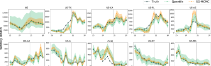
Figure 3. One week ahead COVID-19 incident death forecasting at the country level and 9 states in the United States with the heaviest death tolls from week 23 to week 37.

5.4. Forecasting Performances

Table 2 compares the forecasting performances for 6 UQ methods across three different applications: (1) PM 2.5 forecasting for next 12 - 48 hours on the hourly recorded weather and air quality dataset, (2) 15min - 1 hour ahead traffic speed forecasting on METR-LA and (3) four weeks ahead mortality forecasting on COVID-19. Performances for air quality are aggregated for the entire sequence following the KDD competition standard. Others are reported with the corresponding timestamp.

Across the applications, we observe Bayesian method (SG-MCMC) leads to better prediction accuracy in MAE, even outperforming the point estimation models. On the other hand, frequentist methods generally outperform Bayesian methods for the inference of $95\%$ confidence intervals in MIS.

In specific, directly minimizing MIS score function achieves the best performance in MIS, which is expected. Quantile regression has a similar performance to the $\mathrm{MIS}$-regression, but under-performs in both MAE and MIS. SQ enjoys good prediction accuracy, but has a larger MIS score compared to $\mathrm{MIS}$-regression. MC dropout has relatively good MAE, but the MIS scores are often the highest among all UQ methods.

We note that bootstrap still under-performs most methods due to the limited amount of samples we have. SQ regression helps avoid the confidence interval crossing issue. However, it suffers from a large MIS due to the small number of knots for linear spline quantile function construction. For MC dropout, its prediction accuracy is relatively robust but its MIS is unsatisfactory.

5.5. Forecasts Visualization

We visualize the forecasts of Quantile regression (F) and SG-MCMC (B) for three different tasks in Figure 3,  3,  3. Black solid lines indicate the ground truth. Green lines are the quantile regression predictions and orange lines are the forecasts from SG-MCMC. The shades represent the estimated $95\%$ confidence intervals. In general, we can see that Bayesian method SG-MCMC generates mean predictions much closer to the ground truth but often comes with narrower credible intervals. For example, in PM 2.5 prediction, the confidence intervals of SG-MCMC fail to cover the ground truth for both 24 and 48 hours prediction on 03/06 to 03/08.

On the other hand, frequentist method quantile regression typically captures the true values with wider confidence interval bounds. This corresponds to its low MIS score reported in Table 2. Among all the tasks, the confidence interval bounds of quantile regression generally capture ground truth with $95\%$ probability. For COVID-19 forecasting, quantile regression suffers from limited amount of samples, occasionally resulting in poor performances in states including Texas (US-TX) and New Jersey (US-NJ).

6. Ablation study

6.1. Sample Complexity: Bootstrap and SG-MCMC

Both bootstrap and SG-MCMC provide asymptotic consistency. Yet the sample complexities are often large for complex datasets. It is clear from Figure 4 that the MIS score decreases as more Monte Carlo samples are drawn for both the bootstrap method and SG-MCMC posterior sampling method, indicating that sample variance is a major contribution to the inaccuracies. More importantly, we observe that the MIS score decreases faster with SG-MCMC than with bootstrap, signaling a smaller sample complexity for SG-MCMC.

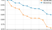
Figure 4. MIS of Bootstrap and SG-MCMC with increasing number of samples for COVID forecasting.

6.2. COVID-19 models: mechanistic, deep learning and hybrid

For COVID-19 mortality forecasting, we have limited amount of data, which is insufficient to train a deep model. Instead, we train our model on the residual between the reported death and the corresponding GLEAM predictions, leading to a hybrid method called DeepGLEAM. Essentially, DeepGLEAM is learning the correction term in the mechanistic GLEAM model. An alternative approach is to directly train our model on the raw incident death counts, which we refer as Deep.

Table 3 shows the RMSE comparison among these models for four weeks ahead forecasting. We can see that DeepGLEAM outperform the mechanics GLEAM model while the Deep model is much worse w.r.t point estimates. In fact, there is a $6.6\%$ improvement for DeepGLEAM and $17\%$ improvement for DeepGLEAM on average from GLEAM.

Horizon $H$	DeepGLEAM	Deep	GLEAM
1W	66.03	239.94	73.59
2W	57.67	213.31	65.46
3W	70.12	189.49	73.75
4W	70.75	161.88	70.16

Table 3. RMSE comparison of different approaches for COVID-19 mortality forecasting

In Figure 5, we visualize the predictions from these three different methods: Deep, GLEAM, and DeepGLEAM models in California. The input data (for training or validation) are from weeks before $34$, and we start the prediction from week $34$, labeled by the vertical dash line. It can be observed that the Deep model fails to predict the dynamics of COVID-19 evolution.

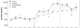
Figure 5. One week ahead COVID-19 forecasts visualization in California. Comparison shown for GEAM, DeepGLEAM and Deep models.

One reason for this phenomenon is the distribution shifts in the epidemiology dynamics. With limited data, deep neural networks do not have enough information to guide their predictions. On the other hand, GLEAM and DeepGLEAM leverage mechanistic knowledge about disease transmission dynamics as inductive bias to infer the underlying dynamics change.

6.3. Anatomy of the performance: Coverage versus accuracy

We conclude from Table 2 that in all the experiments we perform, better performance in MIS is related to not only higher accuracy but also larger confidence bounds. This phenomenon indicates that the deep learning models we consider in this paper generally tend to be overconfident and benefit greatly from better capturing of all sources of variations in the data.

7. Conclusion

We conduct benchmark studies on uncertainty quantification in deep spatiotemporal forecasting from both Bayesian and frequentist perspectives. Through experiments on air quality, traffic and epidemics datasets, we conclude that, with a limited amount of computation, Bayesian methods are typically more robust in mean predictions, while frequentist methods are more effective in covering variations in the data. It is of interest to understand how to best combine Bayesian credible intervals with frequentist confidence intervals to excel in both mean predictions and confidence bounds. Another future direction worth exploring is how to explicitly make use of the spatiotemporal structure of the data in the inference procedures. Current methods we analyze treats minibatches of data as i.i.d. samples. For longer time series with a graph structure, it would be interesting to leverage the spatiotemporal nature of the data to construe efficient inference algorithms (Ma et al., 2017; Aicher et al., 2017; Alaa and van der Schaar, 2020). One limitation of current method is that the confidence interval does not reflect the prediction accuracy. We hypothesize this is due to the limited samples and complexity of the dynamics.

Appendix A Theoretical Analysis

Proof of Proposition 1.

Since the distribution $\mathbb{P}_{Z}$ of $Z$ has probability density $p_{Z}$,

$$\mathrm{MIS}_{\infty}(u,l;\rho) =(u-l)$$

$$+\frac{2}{\rho}\left(\int_{u}^{\infty}(z-u)p_{Z}(z){\textnormal{d}}z+\int_{-\infty}^{l}(l-z)p_{Z}(z){\textnormal{d}}z\right).$$

We demonstrate in the following that the minimum of $\mathrm{MIS}_{\infty}(u,l;\rho)$ is achieved when $u$ and $l$ define the $(1-\rho)$ confidence level.

For simplicity of exposition, we let $p_{Z}$ be symmetric around $0$ and let $l=-u$. Then

$$\mathrm{MIS}_{\infty}(u;\rho)=2u+\frac{4}{\rho}\left(\int_{u}^{\infty}(z-u)p_{Z}(z){\textnormal{d}}z\right).$$

Setting

$$0=\frac{{\textnormal{d}}}{{\textnormal{d}}u}\mathrm{MIS}_{\infty}(u;\rho)=2-\frac{4}{\rho}\left(\int_{u}^{\infty}p_{Z}(z){\textnormal{d}}z\right),$$

we reach the conclusion that the upper bound $u^{*}$ that achieves the minimum MIS satisfies: $\int_{u^{*}}^{\infty}p_{Z}(z){\textnormal{d}}z=\frac{\rho}{2}$. Therefore, $[l^{*},u^{*}]$ defines the $(1-\rho)$ confidence level. ∎

Proof of Proposition 2.

We think about minimizing the MIS score over lower and upper bounds $l$ and $u$, given samples $z_{1},\cdots,z_{N}$ from the posterior distribution:

$$(u,l) ={\arg\min}_{u>l;u,l\in\real}\mathrm{MIS}_{N}(u,l)$$

$$=\underset{u>l;u,l\in\real}{\operatorname*{argmin}}\Big{\{}(u-l)+\frac{2}{\rho N}\sum_{i=1}^{N}((z_{i}-u){\mathds{1}\left\{z_{i}>u\right\}}$$

$$+(l-z_{i}){\mathds{1}\left\{z_{i}<l\right\}})\Big{\}}.$$

We prove in the following that the minimum of MIS score is achieved when we sort $\{z_{1},\cdots,z_{N}\}$ in an increasing order and take $l=z_{\lceil\rho\cdot N/2\rceil}$ and $u=z_{N-\lfloor\rho\cdot N/2\rfloor}$, which define the quantile of the empirical distribution formed by the samples $\{z_{1},\cdots,z_{N}\}$.

We first note that $\mathrm{MIS}_{N}(u,l)$ is a continuous function with respect to $u$ and $l$. Since $\mathrm{MIS}_{N}(u,l)$ is piece-wise linear, we simply need to check that

$$\mathrm{MIS}_{N}(z_{j}^{-},l) =(z_{j}-l)$$

$$+\frac{2}{\rho N}\sum_{i\neq j}\left((z_{i}-u){\mathds{1}\left\{z_{i}>u\right\}}+(l-z_{i}){\mathds{1}\left\{z_{i}<l\right\}}\right)$$

$$=\mathrm{MIS}_{N}(z_{j}^{+},l).$$

The result holds similarly for $l$.

In what follows we prove that $\mathrm{MIS}_{N}(u,l)$ is decreasing in $l$ whenever $l\leq z_{\lceil\rho\cdot N/2\rceil}$. Whenever $l\geq z_{\lceil\rho\cdot N/2\rceil}$, $MIS(u,l)$ is increasing in $l$. We can use similar reasoning to prove that the minimum is achieved when $u=z_{N-\lfloor\rho\cdot N/2\rfloor}$.

Consider derivative of $\mathrm{MIS}_{N}(u,l)$ over $l$

(14) $$\frac{\partial\mathrm{MIS}_{N}(u,l)}{\partial l}=-1+\frac{2}{\rho\cdot N}\sum_{i=1}^{N}\frac{\partial\left((l-z_{i}){\mathds{1}\left\{z_{i}<l\right\}}\right)}{\partial l}.$$

Since

(15) $$(l-z_{i}){\mathds{1}\left\{z_{i}<l\right\}}=\begin{cases}l-z_{i}&\text{if $z_{i}<l$}\\ 0&\text{if $z_{i}\geq l$}\end{cases},$$

(16) $$\frac{\partial\left((l-z_{i}){\mathds{1}\left\{z_{i}<l\right\}}\right)}{\partial l}=\begin{cases}1&\text{if $z_{i}<l$}\\ 0&\text{if $z_{i}\geq l$}\end{cases}.$$

When $l\leq z_{\lceil\rho\cdot N/2\rceil}$, $\frac{2}{\rho\cdot N}\sum_{i=1}^{N}\frac{\partial\left((l-z_{i}){\mathds{1}\left\{z_{i}<l\right\}}\right)}{\partial l}\leq 1$. Hence $\mathrm{MIS}_{N}(u,l)$ is decreasing in $l$ whenever $l\leq z_{\lceil\rho\cdot N/2\rceil}$. Whenever $l\geq z_{\lceil\rho\cdot N/2\rceil}$, $\frac{2}{\rho\cdot N}\sum_{i=1}^{N}\frac{\partial\left((l-z_{i}){\mathds{1}\left\{z_{i}<l\right\}}\right)}{\partial l}\geq 1$, making $\mathrm{MIS}_{N}(u,l)$ increasing in $l$. Therefore, $l=z_{\lceil\rho\cdot N/2\rceil}$ is the minimum of $\mathrm{MIS}_{N}(u,l)$.

The above two facts complete the proof and conclude that

(17) $${\arg\min}_{u>l;u,l\in\real}\mathrm{MIS}_{N}(u,l)=(z_{N-\lfloor\rho\cdot N/2\rfloor},z_{\lceil\rho\cdot N/2\rceil}),$$

which define the quantile of the empirical distribution formed by the samples $\{z_{1},\cdots,z_{N}\}$. ∎

Appendix B Experiment Details

B.1. Point Estimation Model Implementation

For the ConvLSTM experiment on air quality dataset, we concatenate the interpolated PM2.5 at grid level with the weather data and use 24-hour sequence as input to forecast PM2.5 in the next 48 hours. The training data is from January 2nd 2017 to January 31st 2018. We split it into 72-hour sequences. For every sequence, the data is normalized for each channel (temperature, pressure, humidity, wind direction, wind speed, PM2.5). We use one month data from February 1st to February 28th in 2018 for validation and the following month data from March 1st to March 26th for testing, using the first 26 and 24 24-hour records respectively as the input to make the next 48 hour’s PM2.5 forecast.

For the DCRNN model used in traffic dataset, we use two hidden layers of RNN with 64 units. The filter type is a dual random walk and the diffusion step is 2. The learning rate of DCRNN is fixed at $1e^{-2}$ with Adam optimizer. We perform early stopping at 50 epochs.

For the COVID-19 dataset, We use an encoder-decoder sequence to sequence learning framework in the DCRNN structure. The encoder reads as input a $7\times 50\times 4$ tensor that comprises the daily residuals between the observed death number and the GLEAM forecasts for the $50$ US states over $4$ different prediction horizons. It encodes the information in $7$ hidden layers. The decoder produces forecasts of the weekly residuals between the true death number and the GLEAM forecasts for each state for the following $4$ weeks. We perform autoregressive weekly death predictions (from one week ahead to four weeks ahead). The DCRNN model only has one hidden layer of RNN with 8 units to overcome the overfitting problem. The filter type is Laplacian and the diffusion step is 1. The base learning rate of DCRNN is $1e^{-2}$ and decay to $1e^{-3}$ at epoch 13 with Adam optimizer. We have a strict early stopping policy to deal with the overfitting problem. The training stops as the validation error does not improve for three epochs after epoch 13.

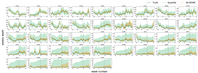
Figure 6. One week ahead COV-19 prediction for the rest of the 41 states in the United States.

Table 4. Performance comparison of different DeepGLEAM Models for COVID-19 mortality forecasting.

Horizon $H$	Metric	Point	Bootstrap	Quantile	SQ	MAE-MIS	MC Drpoout	SG-MCMC
1W	RMSE	68.56	70.73	70.26	73.82	76.32	68.58	62.42
	MIS	—	1216.63	430.72	1299.78	424.49	831.86	715.40
2W	RMSE	59.26	61.69	60.94	65.44	65.39	59.27	51.21
	MIS	—	1135.01	331.94	1272.82	368.20	796.54	727.27
3W	RMSE	70.35	73.27	71.72	73.88	74.95	70.32	66.72
	MIS	—	1464.52	392.66	1559.62	416.23	997.65	930.55
4W	RMSE	72.29	72.41	73.44	70.44	75.16	72.24	68.40
	MIS	—	1482.08	418.77	1586.95	468.49	1034.68	971.55

B.2. Global Epidemic and Mobility Model.

The Global Epidemic and Mobility model (GLEAM) is a stochastic, spatial, age-structured epidemic model based on a metapopulation approach which divides the world into over 3,200 geographic subpopulations constructed using a Voronoi tessellation of the Earth’s surface. Subpopulations are centered around major transportation hubs (e.g. airports) and consist of cells with a resolution of approximately 25 x 25 kilometers (Balcan et al., 2009, 2010; Tizzoni et al., 2012; Zhang et al., 2017b; Chinazzi et al., 2020; Davis et al., 2020). High resolution data are used to define the population of each cell. Other attributes of individual subpopulations, such as age-specific contact patterns, health infrastructure, etc., are added according to available data (Mistry et al., 2020).

GLEAM integrates a human mobility layer - represented as a network - that uses both short-range (i.e., commuting) and long-range (i.e., flight) mobility data from the Offices of Statistics for $30$ countries on $5$ continents as well as the Official Aviation Guide (OAG) and IATA databases (updated in $2021$). The air travel network consists of the daily passenger flows between airport pairs (origin and destination) worldwide mapped to the corresponding subpopulations. Where information is not available, the short-range mobility layer is generated synthetically by relying on the “gravity law” or the more recent “radiation law” both calibrated using real data (Simini et al., 2012).

The model is calibrated to realistically describe the evolution of the COVID-19 pandemic as detailed in (Chinazzi et al., 2020; Davis et al., 2020). Lastly, GLEAM is stochastic and produces an ensemble of possible epidemic outcomes for each set of initial conditions. To account for the potentially different reporting levels of the states, a free parameter Infection Fatality Rate (IFR) multiplier is added to each model. To calibrate and select the most reasonable outcomes, we filter the models by the latest hospitalization trends and confirmed cases trends, and then we select and weight the filtered models using Akaike Information Criterion (Zhang et al., 2017a). The forecast of the evolution of the epidemic is formed by the final ensemble of the selected models.

B.3. Additional Results

Figure 6 visualizes the forecasts of Quantile regression (F) and SG-MCMC(B) for COVID-19 for the rest of the 41 states in U.S. Black solid lines indicate the ground truth. Green lines are the quantile regression predictions and orange lines are the forecasts from SG-MCMC. The shades represent the estimated 95%confidence intervals. In general, we can see that SG-MCMC generates mean predictions much closer to the ground truth but often comes with narrower credible intervals

In addition to autoregressive forecasting, we also build an ensemble DeepGLEAM model by training based on the ensembled data along the forecasting horizon as the output. We use the ensemble DeepGLEAM model which predicts the next 4 weeks death prediction together from the first decoder. Table 4 shows the performance among the UQ methods, which shares similar results with the autoregressive model.

References

- (1)
- Aicher et al. (2017) Chris Aicher, Yi-An Ma, Nick Foti, and Emily B. Fox. 2017. Stochastic gradient MCMC for state space models. SIAM Journal on Mathematics of Data Science (SIMODS) 1 (2017), 555–587.
- Alaa and van der Schaar (2020) AM Alaa and M van der Schaar. 2020. Frequentist Uncertainty in Recurrent Neural Networks via Blockwise Influence Functions. In ICML.
- Amodei et al. (2016) Dario Amodei, Chris Olah, Jacob Steinhardt, Paul Christiano, John Schulman, and Dan Mané. 2016. Concrete problems in AI safety. arXiv preprint arXiv:1606.06565 (2016).
- Askanazi et al. (2018) Ross Askanazi, Francis X Diebold, Frank Schorfheide, and Minchul Shin. 2018. On the comparison of interval forecasts. Journal of Time Series Analysis 39, 6 (2018), 953–965.
- Balcan et al. (2009) Duygu Balcan, Vittoria Colizza, Bruno Gonçalves, Hao Hu, José J Ramasco, and Alessandro Vespignani. 2009. Multiscale mobility networks and the spatial spreading of infectious diseases. Proceedings of the National Academy of Sciences 106, 51 (2009), 21484–21489.
- Balcan et al. (2010) Duygu Balcan, Bruno Gonçalves, Hao Hu, José J Ramasco, Vittoria Colizza, and Alessandro Vespignani. 2010. Modeling the spatial spread of infectious diseases: The GLobal Epidemic and Mobility computational model. Journal of computational science 1, 3 (2010), 132–145.
- Blundell et al. (2015) Charles Blundell, Julien Cornebise, Koray Kavukcuoglu, and Daan Wierstra. 2015. Weight Uncertainty in Neural Network. In ICML. 1613–1622.
- Brier (1950) Glenn W Brier. 1950. Verification of forecasts expressed in terms of probability. Monthly weather review 78, 1 (1950), 1–3.
- Chinazzi et al. (2020) Matteo Chinazzi, Jessica T. Davis, Marco Ajelli, Corrado Gioannini, Maria Litvinova, Stefano Merler, Ana Pastore y Piontti, Kunpeng Mu, Luca Rossi, Kaiyuan Sun, Cécile Viboud, Xinyue Xiong, Hongjie Yu, M. Elizabeth Halloran, Ira M. Longini, and Alessandro Vespignani. 2020. The effect of travel restrictions on the spread of the 2019 novel coronavirus (COVID-19) outbreak. Science 368, 6489 (2020), 395–400.
- Cressie and Wikle (2015) Noel Cressie and Christopher K Wikle. 2015. Statistics for spatio-temporal data. John Wiley & Sons.
- Davis et al. (2020) Jessica T Davis, Matteo Chinazzi, Nicola Perra, Kunpeng Mu, Ana Pastore y Piontti, Marco Ajelli, Natalie E Dean, Corrado Gioannini, Maria Litvinova, Stefano Merler, Luca Rossi, Kaiyuan Sun, Xinyue Xiong, M. Elizabeth Halloran, Ira M Longini, Cécile Viboud, and Alessandro Vespignani. 2020. Estimating the establishment of local transmission and the cryptic phase of the COVID-19 pandemic in the USA. medRxiv (2020).
- Ding et al. (2014) Nan Ding, Youhan Fang, Ryan Babbush, Changyou Chen, Robert D Skeel, and Hartmut Neven. 2014. Bayesian sampling using stochastic gradient thermostats. In NIPS. 3203–3211.
- Dong et al. (2020) Ensheng Dong, Hongru Du, and Lauren Gardner. 2020. An interactive web-based dashboard to track COVID-19 in real time. The Lancet infectious diseases 20, 5 (2020), 533–534.
- Dusenberry et al. (2020) M. Dusenberry, G. Jerfel, Y. Wen, Y.-A. Ma, J. Snoek, K. Heller, B. Lakshminarayanan, and D. Tran. 2020. Efficient and scalable Bayesian neural nets with rank-1 factors. In ICML. 9823–9833.
- Efron and Hastie (2016) Bradley Efron and Trevor Hastie. 2016. Computer Age Statistical Inference. Vol. 5. Cambridge University Press.
- Fort et al. (2019) S. Fort, H. Hu, and B. Lakshminarayanan. 2019. Deep ensembles: A loss landscape perspective. (2019). arXiv:1912.02757.
- Gal and Ghahramani (2016) Yarin Gal and Zoubin Ghahramani. 2016. Dropout as a Bayesian approximation: Representing model uncertainty in deep learning. In ICML. 1050–1059.
- Gal et al. (2017) Yarin Gal, Jiri Hron, and Alex Kendall. 2017. Concrete dropout. In NIPS. 3581–3590.
- Gasthaus et al. (2019) Jan Gasthaus, Konstantinos Benidis, Yuyang Wang, Syama Sundar Rangapuram, David Salinas, Valentin Flunkert, and Tim Januschowski. 2019. Probabilistic forecasting with spline quantile function RNNs. In AISTATS 22. 1901–1910.
- Geng et al. (2019) Xu Geng, Yaguang Li, Leye Wang, Lingyu Zhang, Qiang Yang, Jieping Ye, and Yan Liu. 2019. Spatiotemporal multi-graph convolution network for ride-hailing demand forecasting. In Proceedings of the AAAI conference on artificial intelligence, Vol. 33. 3656–3663.
- Gneiting and Raftery (2007) Tilmann Gneiting and Adrian E Raftery. 2007. Strictly proper scoring rules, prediction, and estimation. Journal of the American statistical Association 102, 477 (2007), 359–378.
- Graves (2011) Alex Graves. 2011. Practical variational inference for neural networks. In NIPS. 2348–2356.
- Hamill and Wilks (1995) Thomas M Hamill and Daniel S Wilks. 1995. A probabilistic forecast contest and the difficulty in assessing short-range forecast uncertainty. Weather and Forecasting 10, 3 (1995), 620–631.
- Heek and Kalchbrenner (2019) Jonathan Heek and Nal Kalchbrenner. 2019. Bayesian Inference for Large Scale Image Classification. (2019). arXiv:1908.03491.
- IATA, International Air Transport Association (2021) IATA, International Air Transport Association. 2021. https://www.iata.org/ https://www.iata.org/.
- Jagadish et al. (2014) Hosagrahar V Jagadish, Johannes Gehrke, Alexandros Labrinidis, Yannis Papakonstantinou, Jignesh M Patel, Raghu Ramakrishnan, and Cyrus Shahabi. 2014. Big data and its technical challenges. Commun. ACM 57, 7 (2014), 86–94.
- Kingma and Dhariwal (2018) Durk P Kingma and Prafulla Dhariwal. 2018. Glow: Generative flow with invertible 1x1 convolutions. In NIPS. 10215–10224.
- Kingma and Welling (2013) Diederik P Kingma and Max Welling. 2013. Auto-encoding variational Bayes. arXiv preprint arXiv:1312.6114 (2013).
- Kipf and Welling (2016) Thomas N Kipf and Max Welling. 2016. Semi-Supervised Classification with Graph Convolutional Networks. (2016).
- Kivaranovic et al. (2020) Danijel Kivaranovic, Kory D Johnson, and Hannes Leeb. 2020. Adaptive, Distribution-Free Prediction Intervals for Deep Networks. In AISTATS. 4346–4356.
- Koenker (2005) R. Koenker. 2005. Quantile Regression. Cambridge University Press.
- Lakshminarayanan et al. (2017) Balaji Lakshminarayanan, Alexander Pritzel, and Charles Blundell. 2017. Simple and scalable predictive uncertainty estimation using deep ensembles. In NIPS. 6402–6413.
- Lee et al. (2015) Stefan Lee, Senthil Purushwalkam, Michael Cogswell, David Crandall, and Dhruv Batra. 2015. Why M heads are better than one: Training a diverse ensemble of deep networks. arXiv:1511.06314 (2015).
- Li et al. (2018) Yaguang Li, Rose Yu, Cyrus Shahabi, and Yan Liu. 2018. Diffusion Convolutional Recurrent Neural Network: Data-Driven Traffic Forecasting. In ICLR.
- Lin et al. (2020) Haoxing Lin, Rufan Bai, Weijia Jia, Xinyu Yang, and Yongjian You. 2020. Preserving Dynamic Attention for Long-Term Spatial-Temporal Prediction. In ACM SIGKDD. 36–46.
- Liu and Shuo (2018) G Liu and S Shuo. 2018. Air quality forecasting using convolutional LSTM.
- Louizos and Welling (2016) Christos Louizos and Max Welling. 2016. Structured and efficient variational deep learning with matrix gaussian posteriors. In ICML. 1708–1716.
- Ma et al. (2015) Yi-An Ma, Tianqi Chen, and Emily Fox. 2015. A complete recipe for stochastic gradient MCMC. In NIPS. 2917–2925.
- Ma et al. (2017) Yi-An Ma, Nicholas J. Foti, and Emily B. Fox. 2017. Stochastic gradient MCMC Methods for hidden Markov models. In ICML. 2265–2274.
- Maddox et al. (2019) Wesley J Maddox, Pavel Izmailov, Timur Garipov, Dmitry P Vetrov, and Andrew Gordon Wilson. 2019. A simple baseline for Bayesian uncertainty in deep learning. In NeurIPS. 13153–13164.
- Matheson and Winkler (1976) James E Matheson and Robert L Winkler. 1976. Scoring rules for continuous probability distributions. Management science 22, 10 (1976), 1087–1096.
- Mistry et al. (2020) Dina Mistry, Maria Litvinova, Matteo Chinazzi, Laura Fumanelli, Marcelo FC Gomes, Syed A Haque, Quan-Hui Liu, Kunpeng Mu, Xinyue Xiong, M Elizabeth Halloran, et al. 2020. Inferring high-resolution human mixing patterns for disease modeling. arXiv preprint arXiv:2003.01214 (2020).
- Neal (2012) Radford M Neal. 2012. Bayesian learning for neural networks. Vol. 118. Springer Science & Business Media.
- OAG, Aviation Worlwide Limited (2021) OAG, Aviation Worlwide Limited. 2021. http://www.oag.com/ http://www.oag.com/.
- Osband et al. (2016) Ian Osband, Charles Blundell, Alexander Pritzel, and Benjamin Van Roy. 2016. Deep Exploration via Bootstrapped DQN. In NIPS. 4026–4034.
- Pearce et al. (2018) Tim Pearce, Alexandra Brintrup, Mohamed Zaki, and Andy Neely. 2018. High-quality prediction intervals for deep learning: A distribution-free, ensembled approach. In ICML. PMLR, 4075–4084.
- Qiu et al. (2019) Xin Qiu, Elliot Meyerson, and Risto Miikkulainen. 2019. Quantifying Point-Prediction Uncertainty in Neural Networks via Residual Estimation with an I/O Kernel. In ICLR.
- Rezende et al. (2014) Danilo Jimenez Rezende, Shakir Mohamed, and Daan Wierstra. 2014. Stochastic backpropagation and approximate inference in deep generative models. arXiv preprint arXiv:1401.4082 (2014).
- Shang et al. (2015) Xiaocheng Shang, Zhanxing Zhu, Benedict Leimkuhler, and Amos J Storkey. 2015. Covariance-Controlled Adaptive Langevin Thermostat for Large-Scale Bayesian Sampling. In NIPS. 37–45.
- Shekhovtsov and Flach (2018) Alexander Shekhovtsov and Boris Flach. 2018. Feed-forward propagation in probabilistic neural networks with categorical and max layers. In ICLR.
- Simini et al. (2012) Filippo Simini, Marta C González, Amos Maritan, and Albert-László Barabási. 2012. A universal model for mobility and migration patterns. Nature 484, 7392 (2012), 96–100.
- Tagasovska and Lopez-Paz (2019) Natasa Tagasovska and David Lopez-Paz. 2019. Single-model uncertainties for deep learning. In NeurIPS. 6417–6428.
- Tizzoni et al. (2012) Michele Tizzoni, Paolo Bajardi, Chiara Poletto, José J Ramasco, Duygu Balcan, Bruno Gonçalves, Nicola Perra, Vittoria Colizza, and Alessandro Vespignani. 2012. Real-time numerical forecast of global epidemic spreading: case study of 2009 A/H1N1pdm. BMC medicine 10, 1 (2012), 165.
- US-EPA (2012) US-EPA. 2012. Revised air quality standards for particle pollution and updates to the Air Quality Index (AQI).
- Vandal et al. (2018) Thomas Vandal, Evan Kodra, Jennifer Dy, Sangram Ganguly, Ramakrishna Nemani, and Auroop R Ganguly. 2018. Quantifying uncertainty in discrete-continuous and skewed data with Bayesian deep learning. In ACM SIGKDD. 2377–2386.
- Wang et al. (2019) Bin Wang, Jie Lu, Zheng Yan, Huaishao Luo, Tianrui Li, Yu Zheng, and Guangquan Zhang. 2019. Deep uncertainty quantification: A machine learning approach for weather forecasting. In ACM SIGKDD. 2087–2095.
- Wang et al. (2016) Hao Wang, Xingjian Shi, and Dit-Yan Yeung. 2016. Natural-parameter networks: A class of probabilistic neural networks. NIPS 29 (2016), 118–126.
- Wang et al. (2017) Yunbo Wang, Mingsheng Long, Jianmin Wang, Zhifeng Gao, and S Yu Philip. 2017. Predrnn: Recurrent neural networks for predictive learning using spatiotemporal lstms. In NIPS. 879–888.
- Welling and Teh (2011) Max Welling and Yee W Teh. 2011. Bayesian learning via stochastic gradient Langevin dynamics. In ICML. 681–688.
- Wen et al. (2017) Ruofeng Wen, Kari Torkkola, Balakrishnan Narayanaswamy, and Dhruv Madeka. 2017. A multi-horizon quantile recurrent forecaster. arXiv preprint arXiv:1711.11053 (2017).
- Wilson and Izmailov (2020) Andrew Gordon Wilson and Pavel Izmailov. 2020. Bayesian Deep Learning and a Probabilistic Perspective of Generalization. arXiv:2002.08791 (2020).
- Xingjian et al. (2015) Shi Xingjian, Zhourong Chen, Hao Wang, Dit-Yan Yeung, Wai-Kin Wong, and Wang-chun Woo. 2015. Convolutional LSTM network: A machine learning approach for precipitation nowcasting. In NIPS. 802–810.
- Yao et al. (2019) Huaxiu Yao, Xianfeng Tang, Hua Wei, Guanjie Zheng, and Zhenhui Li. 2019. Revisiting spatial-temporal similarity: A deep learning framework for traffic prediction. In Proceedings of the AAAI conference on artificial intelligence, Vol. 33. 5668–5675.
- Yao et al. (2018) Huaxiu Yao, Fei Wu, Jintao Ke, Xianfeng Tang, Yitian Jia, Siyu Lu, Pinghua Gong, Jieping Ye, and Zhenhui Li. 2018. Deep multi-view spatial-temporal network for taxi demand prediction. In Proceedings of the AAAI Conference on Artificial Intelligence, Vol. 32.
- Yi et al. (2018) Xiuwen Yi, Junbo Zhang, Zhaoyuan Wang, Tianrui Li, and Yu Zheng. 2018. Deep distributed fusion network for air quality prediction. In ACM SIGKDD. 965–973.
- Yu et al. (2018) Bing Yu, Haoteng Yin, and Zhanxing Zhu. 2018. Spatio-temporal graph convolutional networks: a deep learning framework for traffic forecasting. In Proceedings of the 27th International Joint Conference on Artificial Intelligence. 3634–3640.
- Zhang et al. (2019) Jingzhao Zhang, Tianxing He, Suvrit Sra, and Ali Jadbabaie. 2019. Why gradient clipping accelerates training: A theoretical justification for adaptivity. arXiv:1905.11881 (2019).
- Zhang et al. (2017a) Qian Zhang, Nicola Perra, Daniela Perrotta, Michele Tizzoni, Daniela Paolotti, and Alessandro Vespignani. 2017a. Forecasting seasonal influenza fusing digital indicators and a mechanistic disease model. In Proceedings of the 26th international conference on world wide web. 311–319.
- Zhang et al. (2017b) Qian Zhang, Kaiyuan Sun, Matteo Chinazzi, Ana Pastore y Piontti, Natalie E Dean, Diana Patricia Rojas, Stefano Merler, Dina Mistry, Piero Poletti, Luca Rossi, et al. 2017b. Spread of Zika virus in the Americas. Proceedings of the National Academy of Sciences 114, 22 (2017), E4334–E4343.
- Zhu and Laptev (2017) Lingxue Zhu and Nikolay Laptev. 2017. Deep and confident prediction for time series at uber. In 2017 IEEE International Conference on Data Mining Workshops (ICDMW). IEEE, 103–110.