Permutohedra for knots and quivers

Abstract

The knots-quivers correspondence states that various characteristics of a knot are encoded in the corresponding quiver and the moduli space of its representations. However, this correspondence is not a bijection: more than one quiver may be assigned to a given knot and encode the same information. In this work we study this phenomenon systematically and show that it is generic rather than exceptional. First, we find conditions that characterize equivalent quivers. Then we show that equivalent quivers arise in families that have the structure of permutohedra, and the set of all equivalent quivers for a given knot is parameterized by vertices of a graph made of several permutohedra glued together. These graphs can be also interpreted as webs of dual 3d $\mathcal{N}=2$ theories. All these results are intimately related to properties of homological diagrams for knots, as well as to multi-cover skein relations that arise in counting of holomorphic curves with boundaries on Lagrangian branes in Calabi-Yau three-folds.















CALT-2021-019

1 Introduction

Knots and quivers play an important role in high energy theoretical physics. Knots often arise in the context of topological invariance and can be related to physical objects – such as Wilson loops, defects, and Lagrangian branes – in gauge theories and topological string theory. Quivers may encode interactions of BPS states assigned to their nodes, or the structure of gauge theories. These two seemingly different entities have been recently related by the so-called knots-quivers correspondence KRSS1707short ; KRSS1707long , which identifies various characteristics of knots with those of quivers and moduli spaces of their representations. The knots-quivers correspondence follows from properties of appropriately engineered brane systems in the resolved conifold that represent knots, thus it is intimately related to topological string theory and Gromov-Witten theory EKL1811 ; EKL1910 , and has been further generalized to branes in other Calabi-Yau manifolds PS1811 ; Kimura:2020qns , see also Bousseau:2020fus . Other aspects and proofs (for two-bridge and arborescent knots and links) of the knots-quivers correspondence are discussed in PSS1802 ; SW1711 ; SW2004 ; Kuch2005 .

If there is a correspondence between two types of objects, such as knots and quivers, an important immediate question is how unique both sides of this correspondence are. Examples of two different quivers of the same size that correspond to the same knot were already identified in KRSS1707long , which means that the knots-quivers correspondence is not a bijection. In this paper we study this phenomenon systematically and find conditions that characterize equivalent quivers (i.e. different quivers that correspond to the same knot). It turns out that these conditions lead to interesting local and global structure of the set of equivalent quivers. We stress that equivalent quivers that we consider in this paper are of the same size $m$, such that their nodes are in one-to-one correspondence with generators of HOMFLY-PT homology of a given knot. One can always use certain $q$-identities to construct quivers of larger size that encode the same generating functions of knot polynomials, however this phenomenon has already been studied (see KRSS1707long ; EKL1910 ) and it is not of our primary interest.

Let us thus consider a matrix $C$ of size $m$ (equal to the number of HOMFLY-PT homology generators of a given knot), such that entries $C_{ij}$ are numbers of arrows between nodes $i$ and $j$ of a symmetric quiver corresponding to this knot. We characterize the local equivalence of quivers by showing that some of the quivers equivalent to $C$ are encoded in matrices $C^{\prime}$, such that $C$ and $C^{\prime}$ differ only by a transposition of two elements $C_{ab}$ and $C_{cd}$, whose values differ by one and which satisfy a few additional conditions. From each such equivalent matrix $C^{\prime}$ one can determine another set of equivalent matrices $C^{\prime\prime}$, etc. This procedure produces a closed and connected network of equivalent quivers in a finite number of steps. It follows that any two equivalent quivers from this network differ simply by a sequence of transpositions of elements of their matrices.

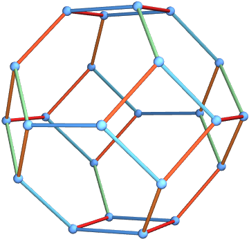
Figure 1: Permutohedron $\Pi_{4}$. Its vertices are labeled by permutations of elements $\{1,2,3,4\}$, and different colors of edges correspond to different types of transpositions $(i\ j)$ (for $1\leq i<j\leq 4$). Vertices connected by an edge differ by one transposition of neighboring elements.

Furthermore, we find that the network of such equivalent quivers has an interesting global structure. We show that equivalent quivers arise in families that form permutohedra. Recall that a permutohedron $\Pi_{n}$ is the $(n-1)$-dimensional polytope, whose vertices are labeled by permutations $\sigma\in S_{n}$ and edges correspond to transpositions of adjacent elements. Permutohedron $\Pi_{2}$ consists of two vertices connected by an edge, $\Pi_{3}$ is a hexagon, and $\Pi_{4}$ is a truncated octahedron shown in figure 1. In our context, each vertex of a permutohedron represents a quiver matrix and each edge connects equivalent quivers (which are related by a transposition of two appropriate elements). Every permutohedron arises from a particular pattern of transpositions of elements of quiver matrices, or equivalently from some particular way of writing a generating function of colored superpolynomials for a given knot. For a given knot, there are typically several ways of writing a generating function of colored superpolynomials, which lead to different permutohedra connected by quivers they share. Examples of such graphs for torus knots $9_{1}$ and $11_{1}$ are shown in figures 2 and 3, and we call them permutohedra graphs.

We find that the above mentioned conditions that characterize equivalent quivers have interesting interpretation in both knot theory and topological string theory. In the knot theory these conditions are related to the structure of the (uncolored and $S^{2}$-colored) HOMFLY-PT homology of a knot in question, and they have a nice graphical manifestation at the level of homological diagrams: they are the center of mass conditions for homology generators. On the other hand, these conditions can be also expressed in terms of multi-cover skein relations that arise in counting of holomorphic curves with boundaries on a Lagrangian brane in Calabi-Yau three-folds. These connections provide a new link between homological invariants of knots, Gromov-Witten theory, and moduli spaces of quiver representations. Moreover, equivalent quivers corresponding to a given knot represent dual 3-dimensional theories with $\mathcal{N}=2$ supersymmetry, analogously as discussed in AFGS1203 ; FGSS1209 ; Chung:2014qpa ; EKL1811 . One can therefore interpret permutohedra graphs as webs of dual 3d $\mathcal{N}=2$ theories.

As mentioned above, the appearance of permutohedra can be interpreted at the level of generating functions of colored superpolynomials. More precisely, we show that each of them can be decomposed into a piece that encodes a given permutohedron, coupled to another piece that itself has a structure of a motivic generating function for a smaller quiver that we refer to as a prequiver. All equivalent quivers corresponding to a given permutohedron are obtained from the same prequiver in the procedure of splitting that involves specifying some particular permutation – so this is the reason why permutohedra arise.

Figure 2: Permutohedra graph for $9_{1}$ torus knot. It consists of two series of permutohedra $\Pi_{2}$, $\Pi_{3}$ and $\Pi_{4}$ connected in the middle, and several other permutohedra $\Pi_{2}$.

Figure 3: Permutohedra graph for $11_{1}$ torus knot. It consists of two series of permutohedra $\Pi_{2}$, $\Pi_{3}$, $\Pi_{4}$ and $\Pi_{5}$ connected in the middle, and several other permutohedra $\Pi_{2}$ and $\Pi_{3}$.

From the above introductory remarks, or simply from figures 2 and 3, it follows that the appearance of equivalent quivers is not an exception, but rather a common and abundant phenomenon. This also means that one should regard as a knot invariant the whole set of equivalent quivers, rather than one particular quiver from this class; moduli spaces of all such equivalent quivers encode the same information about the corresponding knot. The number of equivalent quivers that satisfy the above mentioned conditions grows fast with the size of the homological diagram: it appears that the unknot and trefoil are the only knots such that corresponding quivers are unique, while some knots with 6 or 7 crossings already have over $100\,000$ such equivalent quivers (see the last column of table 1). For a given knot, the number of equivalent quivers that we consider is of the order of the size of the largest permutohedron in the permutohedra graph. For example, we find that the largest permutohedra for $(2,2p+1)$ torus knots are two $\Pi_{p}$, which means that the number of equivalent quivers for this family grows factorially as $2p!$.

Apart from the number of equivalent quivers, in table 1 we also present the number of pairings and symmetries for various knots that we analyze in the paper. By pairings we mean quadruples of generators in the homological diagram that satisfy the center of mass condition mentioned above; this is a necessary, but not sufficient, condition of local equivalence (i.e. equivalence of quiver matrices that differ by one transposition of their elements). On the other hand, by symmetries we mean quadruples of homology generators that satisfy sufficient conditions of local equivalence – the presence of symmetry means that an appropriate transposition of matrix elements indeed produces an equivalent quiver. In particular, we conjecture (and verify to high $p$) that the numbers of pairings and symmetries for $(2,2p+1)$ torus knots are respectively $p^{2}(p-1)/2$ and $p(p^{2}-1)/3$.

Finally, we also extend our analysis to quivers for knot complements Kuch2005 , which encode $\hat{Z}$ invariants for knot complements (also referred to as $F_{K}$ invariants) GM1904 ; Park1909 ; GGKPS20xx . We show that for $(2,2p+1)$ torus knots equivalence conditions that we find in this paper yield an interesting relation between quivers discussed above (that arise in the original knots-quivers correspondence) and quivers for knot complements.

Knot		Pairings	Symmetries	Equivalent quivers
Unknot	$0_{1}$	0	0	1
Torus knots $T_{2,2p+1}$	$3_{1}$	0	0	1
	$5_{1}$	2	2	3
	$7_{1}$	9	8	13
	$9_{1}$	24	20	68
	$11_{1}$	50	40	405
	$13_{1}$	90	70	2 684
	$15_{1}$	147	112	19 557
	⋮	⋮	⋮	⋮
	$(2p+1)_{1}$	$p^{2}(p-1)/2$	$p(p^{2}-1)/3$	$\sim 2p!$
Twists knots $TK_{2|p|+2}$	$4_{1}$	1	1	2
	$6_{1}$	24	16	141
	$8_{1}$	105	61	36 555
Twists knots $TK_{2p+1}$	$5_{2}$	8	6	12
	$7_{2}$	52	34	1 983
Stand-alone examples	$6_{2}$	46	36	3 534
	$6_{3}$	101	72	142 368
	$7_{3}$	86	67	109 636

Table 1: The number of pairings, symmetries, and equivalent quivers that we have found for $(2,2p+1)$ torus knots, twist knots, and $6_{2},6_{3},7_{3}$ knots.

Note that in principle there might exist other equivalent quivers, which are not related by a series of transpositions that we mentioned above (e.g. they might be related by a cyclic permutation of length larger than 2, such that some transpositions of elements of quiver matrix, which arise from a decomposition of such a permutation, do not preserve the partition function). However, based on the evidence discussed in what follows, we conjecture that such equivalent quivers do not arise.

This paper is structured as follows. Section 2 provides necessary background on knot homologies, knots-quivers correspondence, and multi-cover skein relations. In section 3 we focus on local equivalences and formulate the local equivalence theorem, which states that appropriate transpositions of elements of a given quiver matrix lead to equivalent quivers. In section 4 we discuss how these local equivalences lead to the global structure: we show that equivalent quivers arise in families that form permutohedra which are glued into larger graphs that parametrize all equivalent quivers for a given knot. In section 5 we present examples of such a global structure and illustrate how permutohedra of equivalent quivers arise and are glued together for various knots. In turn, in section 6 we consider examples of local equivalences and determine them for some particular quivers for infinite families of $(2,2p+1)$ torus knots and twist knots, as well as $6_{2},6_{3}$ and $7_{3}$ knots. Section 7 reveals relations of our results to knot complement quivers and $F_{K}$ invariants. In the appendix we present the lists of all equivalent quiver matrices for knots $5_{2}$ and $7_{1}$, as well as particular choices of quiver matrices for infinite classes of twist knots.

2 Prerequisites

In this section we summarize the background material on knot homologies, knots-quivers correspondence, and multi-cover skein relations, as well as introduce the notation that will be used throughout the paper.

2.1 Knot homologies

The knots-quivers correspondence, which is of our main interest in this work, is inherently related to knot homologies. Let us therefore present first a few basic facts about them. We are especially interested in colored HOMFLY-PT homologies, denoted $\mathcal{H}^{R}_{ijk}(K)$ for a knot $K$, where $R$ is a representation (labeled by a Young diagram) referred to as the color DGR0505 ; GS . In this paper we only consider symmetric representations $R=S^{r}$, and in various formulae we simply use the label $r$ instead of $S^{r}$. In particular, by $\mathscr{G}_{r}(K)$ we denote the set of generators of the $S^{r}$-colored homology. While explicit construction of colored HOMFLY-PT homologies has not been provided to date, strong constraints on their structure follow from conjectural properties of associated differentials that relate various generators. In particular, these constraints enable computation of colored superpolynomials and HOMFLY-PT polynomials for various knots. Colored superpolynomials are defined as follows:

$$P_{r}(a,q,t)=\sum_{i,j,k}a^{i}q^{j}t^{k}\textrm{dim}\mathcal{H}^{S^{r}}_{ijk}(K)\equiv\sum_{i\in\mathscr{G}_{r}(K)}a^{a^{(r)}_{i}}q^{q^{(r)}_{i}}t^{t^{(r)}_{i}},$$ (1)

where variables $a$ and $q$ are those that appear in HOMFLY-PT polynomials, $t$ is the refinement (Poincaré) parameter, and we refer to triples $(a^{(r)}_{i},q^{(r)}_{i},t^{(r)}_{i})$ as homological degrees of the generator $i\in\mathscr{G}_{r}(K)$. In the uncolored case $r=1$ we simply write $(a_{i},q_{i},t_{i})\equiv(a^{(1)}_{i},q^{(1)}_{i},t^{(1)}_{i})$. For a large class of knots the linear combination $t_{i}-a_{i}-q_{i}/2$ is constant for each $i\in\mathscr{G}_{1}(K)$; such knots are called thin DGR0505 .

For a given color $r$, it is useful to plot colored HOMFLY-PT generators on a planar diagram, such that the generator $i\in\mathscr{G}_{r}(K)$ is represented by a dot in position $(q^{(r)}_{i},a^{(r)}_{i})$ (and possibly decorated by the value $t^{(r)}_{i}$). The structure of differentials mentioned above also imposes constraints on the form of such diagrams. In particular, in the uncolored case all generators are assembled into two types of structures, referred to as a zig-zag and a diamond GS . The zig-zag consists of an odd number of generators, while each diamond consists of four generators. The homological diagram for each knot consists of one zig-zag and some number of diamonds. For example, homological diagrams for $(2,2p+1)$ torus knots consist of only one zig-zag made of $2p+1$ generators, while a diagram for $4_{1}$ knot consists of one diamond and a zig-zag made of only one dot. We will present examples of homological diagrams for these and other knots in what follows.

For $t=-1$ colored superpolynomials reduce to colored HOMFLY-PT polynomials that take form of the Euler characteristic

$$P_{r}(a,q)=P_{r}(a,q,-1)=\sum_{i,j,k}a^{i}q^{j}(-1)^{k}\textrm{dim}\mathcal{H}^{S^{r}}_{ijk}(K).$$ (2)

We stress that by $P_{r}(a,q,t)$ and $P_{r}(a,q)$ we denote reduced polynomials (equal to 1 for the unknot). We use this normalization throughout the paper except section 7, where using the unreduced normalization is more appropriate. We also consider generating functions of colored superpolynomials and colored HOMFLY-PT polynomials for defined by

$$P_{K}(x,a,q,t)=\sum_{r=0}^{\infty}\frac{x^{r}}{(q^{2};q^{2})_{r}}P_{r}(a,q,t),\qquad\quad P_{K}(x,a,q)=\sum_{r=0}^{\infty}\frac{x^{r}}{(q^{2};q^{2})_{r}}P_{r}(a,q).$$ (3)

Including $q$-Pochhammer symbols $(q^{2};q^{2})_{r}=\prod_{i=1}^{r}(1-q^{2i})$ in denominators provides a proper normalization for the knots-quivers correspondence as defined in KRSS1707short ; KRSS1707long .

2.2 Knots-quivers correspondence

The knots-quivers correspondence is the statement that to a given knot one can assign a quiver in such a way that various characteristics of the knot are expressed in terms of invariants of this quiver (or invariants of moduli spaces of its representations). As already noticed in KRSS1707long , this correspondence is not a bijection, and several quivers may correspond to the same knot. In this work we explain how to identify all such equivalent quivers and reveal the intricate structure they form. However, let us first present relevant background on quiver representation theory, and explain how it relates to knots.

A quiver $Q=(Q_{0},Q_{1})$ consists of a set of nodes $Q_{0}$ and a set of arrows $Q_{1}$. Each arrow connects either two different nodes, or a node to itself – in the latter case it is called a loop. We denote by $C_{ij}$ the number of arrows from the node $i$ to the node $j$, and treat it as an element of a matrix $C$. Quivers that arise in knots-quivers correspondence are symmetric, which means that for each arrow $i\to j$ for $i,j\in Q_{0}$ there exists an arrow in the opposite direction $j\to i$; in this case the matrix $C$ is symmetric.

In quiver representation theory one is interested in the structure of moduli spaces of quiver representations. Let us consider a symmetric quiver $Q$ with $m$ nodes and arrows determined by a matrix $C$. We assign to each node $i$ a complex vector space of dimension $d_{i}$; the $m$-tuple $\boldsymbol{d}=(d_{1},\ldots,d_{m})$ is referred to as the dimension vector. Furthermore, for such a quiver we construct the following generating series

$$P_{Q}(\boldsymbol{x},q)=\sum_{\boldsymbol{d}}(-q)^{\boldsymbol{d}\cdot C\cdot\boldsymbol{d}}\frac{\boldsymbol{x}^{\boldsymbol{d}}}{(q^{2};q^{2})_{\boldsymbol{d}}}\equiv\sum_{d_{1},\ldots,d_{m}\geq 0}(-q)^{\sum_{i,j=1}^{m}C_{ij}d_{i}d_{j}}\frac{x_{1}^{d_{1}}\cdots x_{m}^{d_{m}}}{(q^{2};q^{2})_{d_{1}}\cdots(q^{2};q^{2})_{d_{m}}},$$ (4)

where $\boldsymbol{x}=(x_{1},\ldots,x_{m})$ are referred to as quiver generating parameters. It turns out that this generating function encodes motivic Donaldson-Thomas invariants $\Omega_{d_{1},\ldots,d_{m};j}$ of quiver $Q$, i.e. appropriately defined intersection Betti numbers of moduli spaces of representations of $Q$, for all dimension vectors $\boldsymbol{d}$. These invariants are encoded in the following product decomposition of (4):

$$P_{Q}(\boldsymbol{x},q)=\prod_{(d_{1},\ldots,d_{m})\neq 0}\prod_{j\in\mathbb{Z}}\prod_{k\geq 0}\Big{(}1-(x_{1}^{d_{1}}\cdots x_{m}^{d_{m}})q^{2k+j+1}\Big{)}^{(-1)^{j+1}\Omega_{d_{1},\ldots,d_{m};j}}.$$ (5)

It was postulated in KS1006 and proven in Efi12 that motivic Donaldson-Thomas invariants $\Omega_{d_{1},\ldots,d_{m};j}$ are non-negative integers.

The knots-quivers correspondence was motivated by the observation that generating series of colored knot polynomials (3) can be written in the form (4) for appropriate specialization of generating parameters $x_{i}$. This statement was proven in various examples in KRSS1707long , for two-bridge knots in SW1711 , and for arborescent knots in SW2004 . The relation between (3) and (4) has various interesting consequences. For example, it follows that Ooguri-Vafa invariants of a knot OV9912 are expressed in terms of motivic Donaldson-Thomas invariants; as the latter invariants are proven to be integer, it follows that that Ooguri-Vafa invariants are also integer, as has been suspected for a long time. On the other hand, if all colored superpolynomials can be expressed in the form (4), it follows that all of them are encoded in a finite number of parameters, i.e. the elements of the matrix $C$ and additional parameters that arise in the specialization of $x_{i}$. Let us now formulate the knots-quivers correspondence in all details, in a way appropriate for the perspective of this work.

Definition 1.

We say that the quiver $Q$ corresponds to the knot $K$ if $Q$ is symmetric and there exists a bijection

$$Q_{0}\ni i\longleftrightarrow i\in\mathscr{G}_{1}(K)$$ (6)

such that

$$\left.P_{Q}(\boldsymbol{x},q)\right|_{(-q)^{C_{ii}}x_{i}=xa^{a_{i}}q^{q_{i}}t^{t_{i}}}=P_{K}(x,a,q,t)\quad and\quad C_{ii}=t_{i}.$$ (7)

The substitution $(-q)^{C_{ii}}x_{i}=xa^{a_{i}}q^{q_{i}}t^{t_{i}}$ following the bijection (6) is called the knots-quivers change of variables. Denoting $a^{a_{i}}q^{q_{i}-C_{ii}}(-t)^{C_{ii}}$ as $\lambda_{i}$, we can write it shortly as

$$x_{i}=x\lambda_{i}\qquad\textrm{or}\qquad\boldsymbol{x}=x\boldsymbol{\lambda}.$$ (8)

The above correspondence can be also reduced to the level of HOMFLY-PT polynomials, simply by putting $t=-1$ in the knots-quivers change of variables. Note that the above formulation differs from the original one KRSS1707short ; KRSS1707long that does not require bijectivity, only the existence of $\{a_{i},q_{i}\}_{i\in Q_{0}}$ allowing (7). In consequence, transformations enlarging the quiver and preserving the generating function – forbidden by definition 1 – are allowed in KRSS1707short ; KRSS1707long . Therefore, $Q$ corresponding to $K$ in the sense of the definition 1 is the minimal quiver in the original sense of KRSS1707short ; KRSS1707long . One can also define a generalized knots-quivers correspondence EKL1811 , which allows for $x_{i}=x^{n_{i}}\lambda_{i}$ (possibly with $n_{i}>1$), but we do not consider it here.

2.3 Multi-cover skein relations and quivers

Let us now change perspective to that of curve counting for topological strings. It is natural to view holomorphic curves in a Calabi-Yau three-fold with boundary on a Lagrangian $L$ as deforming Chern-Simons theory on $L$ (see Wit92 ). In ES1901 this perspective was used to give a new mathematical approach to open curve counts. Then, EKL1910 showed that the invariance of generalized holomorphic curve counts under bifurcations of basic disks – called multi-cover skein relation – generates quiver degeneracies, i.e. implies the existence of different quivers corresponding to the same knot.

One can visualize the multi-cover skein relation as resolving the intersection between disk boundaries, see figure 4. Using the language of EKL1811 , it can be adapted to quivers as the equality of motivic generating series of two quivers shown at the bottom of figure 4, where each basic disc corresponds to the quiver node, and the linking number corresponds to the number of arrows. Physically, it corresponds to the duality between two 3d $\mathcal{N}=2$ theories and has an interesting relations with the wall-crossing from KS0811 ; KS1006 . More details can be found in EKL1910 .

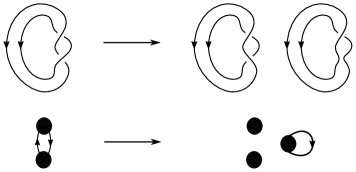
Figure 4: Multi-cover skein relation on linking disks (top) and dual quiver description (bottom) EKL1910 .

The phenomenon presented in figure 4 is the simplest example of unlinking. From the perspective of BPS states, it corresponds to reinterpreting the bound state made of two basic states as an independent basic state. In terms of quivers, it means removing one pair of arrows which encode the interaction leading to a bound state and adding a new node. Adapting EKL1910 to our notation, we define the general case of unlinking in the following way:

Definition 2.

Consider a symmetric quiver $Q$ and fix $a,b\in Q_{0}$. The unlinking of nodes $a,b$ is defined as a transformation of $Q$ leading to a new quiver $\widetilde{Q}$ such that:

• There is a new node $n$: $\widetilde{Q}_{0}=Q_{0}\cup n$.

• The number of arrows of the new quiver is given by

  $$\widetilde{C}_{ab} =C_{ab}-1, \widetilde{C}_{nn} =C_{aa}+2C_{ab}+C_{bb}-1,$$ (9)

  $$\widetilde{C}_{in} =C_{ai}+C_{bi}-\delta_{ai}-\delta_{bi}, \widetilde{C}_{ij} =C_{ij}\quad\textrm{for all other cases,}$$

  where $\delta_{ij}$ is a Kronecker delta.

One can check that quivers on the left- and right-hand side of figure 4 correspond respectively to

$$C=\left[\begin{array}[]{cc}C_{aa}&C_{ab}\\ C_{ba}&C_{bb}\end{array}\right]=\left[\begin{array}[]{cc}0&1\\ 1&0\end{array}\right]\qquad\longrightarrow\qquad\widetilde{C}=\left[\begin{array}[]{ccc}\widetilde{C}_{aa}&\widetilde{C}_{ab}&\widetilde{C}_{an}\\ \widetilde{C}_{ba}&\widetilde{C}_{bb}&\widetilde{C}_{bn}\\ \widetilde{C}_{na}&\widetilde{C}_{nb}&\widetilde{C}_{nn}\end{array}\right]=\left[\begin{array}[]{ccc}0&0&0\\ 0&0&0\\ 0&0&1\end{array}\right].$$ (10)

For us, the most important result of EKL1910 is the following statement:

Theorem 3 (Ekholm, Kucharski, Longhi).

The unlinking accompanied by the substitution $x_{n}=q^{-1}x_{a}x_{b}$ preserves the motivic generating function of the quiver:

$$P_{Q}(\boldsymbol{x},q)=\left.P_{\widetilde{Q}}(\boldsymbol{x},q)\right|_{x_{n}=q^{-1}x_{a}x_{b}}.$$ (11)

In section 3.3 we use it to prove the local equivalence theorem.

3 Local equivalence of quivers

In this section we show that for a given quiver of size $m$ (equal to the number of HOMFLY-PT generators of the corresponding knot), encoded in a symmetric matrix $C$, there exist equivalent quivers such that their matrices differ from $C$ only by a transposition of two non-diagonal elements $C_{ab}$ and $C_{cd}$, as long as the values of these two elements differ by 1 and certain extra conditions are met. This is the phenomenon that we refer to as local equivalence of quivers. In the next sections we show that these local equivalences give rise to an intricate global structure whose building blocks are permutohedra, and provide various examples of this phenomenon.

We start from introducing an equivalence relation that describes quiver degeneracies in a natural way.

Definition 4.

Assume that quiver $Q$ corresponds to the knot $K$ and quiver $Q^{\prime}$ corresponds to the knot $K^{\prime}$ in the sense of the definition 1. Then we define

$$Q\sim Q^{\prime}\Longleftrightarrow K\textrm{ and }K^{\prime}\textrm{ have the~{}same colored HOMFLY-PT homology.}$$ (12)

In the rest of the paper we refer to the simplest and most common version of (12), namely $K=K^{\prime}$. However, each time we write that two (or more) quivers correspond to the same knot, we keep in mind that another knot with the same colored HOMFLY-PT homology would lead to the same equivalence class of quivers.

3.1 Analysis of possible equivalences

Let us study when two quivers $Q$ and $Q^{\prime}$ can correspond to the same knot $K$. Using definition 1, we start from

$$P_{K}(x,a,q,t)=\left.P_{Q}(\boldsymbol{x},q)\right|_{\boldsymbol{x}=x\boldsymbol{\lambda}}=\left.P_{Q^{\prime}}(\boldsymbol{x},q)\right|_{\boldsymbol{x}=x\boldsymbol{\lambda}^{\prime}}$$ (13)

with

$$\lambda_{i}=\lambda^{\prime}_{i}=a^{a_{i}}q^{q_{i}-C_{ii}}(-t)^{C_{ii}},\quad C_{ii}=t_{i}\quad\forall i\in Q_{0}=Q^{\prime}_{0}.$$ (14)

We will analyze equation  (13) order by order in $x$. The linear one holds automatically, so let us focus on terms proportional to $x^{2}$:

$$\begin{split}\frac{P_{2}(a,q,t)x^{2}}{(1-q^{2})(1-q^{4})}&=\sum_{i\in Q_{0}}\frac{(-q)^{4C_{ii}}x^{2}\lambda_{i}^{2}}{(1-q^{2})(1-q^{4})}+\sum_{i,j\in Q_{0},i\neq j}\frac{(-q)^{C_{ii}+2C_{ij}+C_{jj}}x^{2}\lambda_{i}\lambda_{j}}{(1-q^{2})(1-q^{2})}\\ &=\sum_{i\in Q^{\prime}_{0}}\frac{(-q)^{4C_{ii}}x^{2}\lambda_{i}^{2}}{(1-q^{2})(1-q^{4})}+\sum_{i,j\in Q^{\prime}_{0},i\neq j}\frac{(-q)^{C_{ii}+2C^{\prime}_{ij}+C_{jj}}x^{2}\lambda_{i}\lambda_{j}}{(1-q^{2})(1-q^{2})},\end{split}$$ (15)

where we used (14) to write $\lambda_{i}=\lambda^{\prime}_{i}$ and $C_{ii}=C^{\prime}_{ii}$. In consequence, the only difference between $Q$ and $Q^{\prime}$ can appear in non-diagonal terms $C_{ij}$ and $C^{\prime}_{ij}$. Since equation (15) needs to hold for all $a$ and $t$ (which are independent from $C_{ij}$ and $C^{\prime}_{ij}$), we require the equality between coefficients of each monomial in these variables. The only possibility of having $Q\neq Q^{\prime}$ satisfying (13) comes from $C_{ij}\neq C^{\prime}_{ij}$ which however lead to the same coefficient of each monomial in $a$ and $t$ on both sides. The way $q$-monomials on both sides are matched can be described by permutations of terms in the coefficient of each monomial in $a$ and $t$.

Let us focus on the simplest non-trivial case. We assume that each coefficient of monomials in $a$ and $t$ has only one term except from the expression corresponding to $\lambda_{a}\lambda_{b}$ and $\lambda_{c}\lambda_{d}$. This means that we require $\lambda_{a}\lambda_{b}=q^{2s}\lambda_{c}\lambda_{d}$ for some $s\in\mathbb{Z}$ and $\lambda_{a}$, $\lambda_{b}$, $\lambda_{c}$, $\lambda_{d}$ being pairwise different. (Note that for thin knots we immediately know that $s=0$.) Therefore, we get $C_{ij}=C^{\prime}_{ij}\;\forall i,j\in Q_{0}\backslash\{a,b,c,d\}$ and (15) can be reduced to

$$\lambda_{a}\lambda_{b}(-q)^{C_{aa}+C_{bb}}\bigg{(}q^{2C_{ab}}+q^{-2s+2C_{cd}}\bigg{)}=\lambda_{a}\lambda_{b}(-q)^{C_{aa}+C_{bb}}\left(q^{2C^{\prime}_{ab}}+q^{-2s+2C^{\prime}_{cd}}\right),$$ (16)

where we used $C_{aa}+C_{bb}=C_{cc}+C_{dd}$ that comes from the comparison of $t$ powers in $\lambda_{a}\lambda_{b}=q^{2s}\lambda_{c}\lambda_{d}$. In consequence, there is only one non-trivial way to satisfy (15), namely

$$C^{\prime}_{ab}=C_{cd}-s,\quad C^{\prime}_{cd}=C_{ab}+s.$$ (17)

Using the language of permutations of terms in the generating function, this corresponds to the transposition $\lambda_{a}\lambda_{b}(-q)^{C_{aa}+2C_{ab}+C_{bb}}$ $\leftrightarrow$ $\lambda_{c}\lambda_{d}(-q)^{C_{cc}+2C_{cd}+C_{dd}}$. For $s=0$ it translates to the transposition of matrix entries $C_{ab}\leftrightarrow C_{cd}$.

Let us continue the analysis of the simplest non-trivial case and check what conditions come from the cubic order of (13). In order to save space, we start from examining where differences between $\left.P_{Q}(\boldsymbol{x},q)\right|_{x_{i}=x\lambda_{i}}$ and $\left.P_{Q^{\prime}}(\boldsymbol{x},q)\right|_{x_{i}=x\lambda_{i}}$ can arise. The general formula reads

$$\begin{split}\frac{P_{3}(a,q,t)x^{3}}{(1-q^{2})(1-q^{4})(1-q^{6})}&=\sum_{i\in Q_{0}}\frac{(-q)^{9C_{ii}}x^{3}\lambda_{i}^{3}}{(1-q^{2})(1-q^{4})(1-q^{6})}\\ &+\sum_{i,j\in Q{}_{0},i\neq j}\frac{(-q)^{4C_{ii}+4C_{ij}+C_{jj}}x^{3}\lambda_{i}^{2}\lambda_{j}}{(1-q^{2})(1-q^{4})(1-q^{2})}\\ &+\sum_{i,j,k\in Q{}_{0},i\neq j\neq k}\frac{(-q)^{C_{ii}+2C_{ij}+C_{jj}+2C_{jk}+C_{kk}+2C_{ik}}x^{3}\lambda_{i}\lambda_{j}\lambda_{k}}{(1-q^{2})(1-q^{2})(1-q^{2})},\end{split}$$ (18)

so we have to look for terms containing $\lambda_{a}\lambda_{b}$ or $\lambda_{c}\lambda_{d}$. They are given by

$$\begin{split}\frac{x^{3}\lambda_{a}\lambda_{b}}{(1-q^{2})(1-q^{4})(1-q^{6})}&\Big{[}(-q)^{4C_{aa}+4C^{\prime}_{ab}+C_{bb}}\lambda_{a}+(-q)^{4C_{bb}+4C^{\prime}_{ab}+C_{aa}}\lambda_{b}\\ &+(1+q^{2})(-q)^{C_{aa}+2C^{\prime}_{ab}+C_{bb}+2C_{bc}+C_{cc}+2C_{ac}}\lambda_{c}\\ &+(1+q^{2})(-q)^{C_{aa}+2C^{\prime}_{ab}+C_{bb}+2C_{bd}+C_{dd}+2C_{ad}}\lambda_{d}\\ &+(1+q^{2})\sum_{i\in Q_{0}\backslash\{a,b,c,d\}}(-q)^{C_{aa}+2C^{\prime}_{ab}+C_{bb}+2C_{bi}+C_{ii}+2C_{ai}}\lambda_{i}\Big{]}\end{split}$$ (19)

and

$$\begin{split}\frac{x^{3}\lambda_{c}\lambda_{d}}{(1-q^{2})(1-q^{4})(1-q^{6})}&\Big{[}(-q)^{4C_{cc}+4C^{\prime}_{cd}+C_{dd}}\lambda_{c}+(-q)^{4C_{dd}+4C^{\prime}_{cd}+C_{dd}}\lambda_{d}\\ &+(1+q^{2})(-q)^{C_{cc}+2C^{\prime}_{cd}+C_{dd}+2C_{ad}+C_{aa}+2C_{ac}}\lambda_{a}\\ &+(1+q^{2})(-q)^{C_{cc}+2C^{\prime}_{cd}+C_{dd}+2C_{bd}+C_{bb}+2C_{bc}}\lambda_{b}\\ &+(1+q^{2})\sum_{i\in Q_{0}\backslash\{a,b,c,d\}}(-q)^{C_{cc}+2C^{\prime}_{cd}+C_{dd}+2C_{di}+C_{ii}+2C_{ci}}\lambda_{i}\Big{]}\end{split}$$ (20)

for $\left.P_{Q^{\prime}}(\boldsymbol{x},q)\right|_{\boldsymbol{x}=x\boldsymbol{\lambda}}$ and analogous terms without prime symbols for $\left.P_{Q}(\boldsymbol{x},q)\right|_{\boldsymbol{x}=x\boldsymbol{\lambda}}$. Since $\lambda_{a}\lambda_{b}=q^{2s}\lambda_{c}\lambda_{d}$, imposing the equality between $\left.P_{Q^{\prime}}(\boldsymbol{x},q)\right|_{\boldsymbol{x}=x\boldsymbol{\lambda}}$ and $\left.P_{Q}(\boldsymbol{x},q)\right|_{\boldsymbol{x}=x\boldsymbol{\lambda}}$ implies conditions for sums of terms from both (19) and (20) for $\lambda_{a}$, $\lambda_{b}$, $\lambda_{c}$, $\lambda_{d}$ and each $\lambda_{i}$, $i\in Q_{0}\backslash\{a,b,c,d\}$:

$$\begin{split}\lambda_{a}&\Big{[}(-q)^{4C_{aa}+4C^{\prime}_{ab}+C_{bb}+2s}+(1+q^{2})(-q)^{C_{cc}+2C^{\prime}_{cd}+C_{dd}+2C_{ad}+C_{aa}+2C_{ac}}\Big{]}\\ &=\lambda_{a}\Big{[}(-q)^{4C_{aa}+4C_{ab}+C_{bb}+2s}+(1+q^{2})(-q)^{C_{cc}+2C_{cd}+C_{dd}+2C_{ad}+C_{aa}+2C_{ac}}\Big{]},\end{split}$$ (21)

$$\begin{split}\lambda_{b}&\Big{[}(-q)^{4C_{bb}+4C^{\prime}_{ab}+C_{aa}+2s}+(1+q^{2})(-q)^{C_{cc}+2C^{\prime}_{cd}+C_{dd}+2C_{bd}+C_{bb}+2C_{bc}}\Big{]}\\ &=\lambda_{b}\Big{[}(-q)^{4C_{bb}+4C_{ab}+C_{aa}+2s}+(1+q^{2})(-q)^{C_{cc}+2C_{cd}+C_{dd}+2C_{bd}+C_{bb}+2C_{bc}}\Big{]},\end{split}$$ (22)

$$\begin{split}\lambda_{c}&\Big{[}(-q)^{4C_{cc}+4C^{\prime}_{cd}+C_{dd}}+(1+q^{2})(-q)^{C_{aa}+2C^{\prime}_{ab}+C_{bb}+2C_{bc}+C_{cc}+2C_{ac}+2s}\Big{]}\\ &=\lambda_{c}\Big{[}(-q)^{4C_{cc}+4C_{cd}+C_{dd}}+(1+q^{2})(-q)^{C_{aa}+2C_{ab}+C_{bb}+2C_{bc}+C_{cc}+2C_{ac}+2s}\Big{]},\end{split}$$ (23)

$$\begin{split}\lambda_{d}&\Big{[}(-q)^{4C_{dd}+4C^{\prime}_{cd}+C_{cc}}+(1+q^{2})(-q)^{C_{aa}+2C^{\prime}_{ab}+C_{bb}+2C_{bd}+C_{dd}+2C_{ad}+2s}\Big{]}\\ &=\lambda_{d}\Big{[}(-q)^{4C_{dd}+4C_{cd}+C_{cc}}+(1+q^{2})(-q)^{C_{aa}+2C_{ab}+C_{bb}+2C_{bd}+C_{dd}+2C_{ad}+2s}\Big{]},\end{split}$$ (24)

$$\begin{split}\lambda_{i}&\Big{[}(-q)^{C_{aa}+2C^{\prime}_{ab}+C_{bb}+2C_{bi}+C_{ii}+2C_{ai}+2s}+(-q)^{C_{cc}+2C^{\prime}_{cd}+C_{dd}+2C_{di}+C_{ii}+2C_{ci}}\Big{]}\\ &=\lambda_{i}\Big{[}(-q)^{C_{aa}+2C_{ab}+C_{bb}+2C_{bi}+C_{ii}+2C_{ai}+2s}+(-q)^{C_{cc}+2C_{cd}+C_{dd}+2C_{di}+C_{ii}+2C_{ci}}\Big{]}.\end{split}$$ (25)

In each equation we have to match three $q$-monomials on both sides in a non-trivial way. For example, in (21) we must take

$$4C_{aa}+4C^{\prime}_{ab}+C_{bb}+2s =C_{cc}+2C_{cd}+C_{dd}+2C_{ad}+C_{aa}+2C_{ac}+2,$$

$$C_{cc}+2C^{\prime}_{cd}+C_{dd}+2C_{ad}+C_{aa}+2C_{ac} =4C_{aa}+4C_{ab}+C_{bb}+2s,$$ (26)

$$C_{cc}+2C^{\prime}_{cd}+C_{dd}+2C_{ad}+C_{aa}+2C_{ac}+2 =C_{cc}+2C_{cd}+C_{dd}+2C_{ad}+C_{aa}+2C_{ac},$$

or

$$4C_{aa}+4C^{\prime}_{ab}+C_{bb}+2s =C_{cc}+2C_{cd}+C_{dd}+2C_{ad}+C_{aa}+2C_{ac},$$

$$C_{cc}+2C^{\prime}_{cd}+C_{dd}+2C_{ad}+C_{aa}+2C_{ac} =C_{cc}+2C_{cd}+C_{dd}+2C_{ad}+C_{aa}+2C_{ac}+2,$$

$$C_{cc}+2C^{\prime}_{cd}+C_{dd}+2C_{ad}+C_{aa}+2C_{ac}+2 =4C_{aa}+4C_{ab}+C_{bb}+2s.$$ (27)

Analogous matching for equations for (22-24), combined with $C_{aa}+C_{bb}=C_{cc}+C_{dd}$ and (17), leads to two possible ways for non-trivial pairwise cancellation:

$$\begin{aligned} C_{ab}+s=&\ C_{cd}-1,\\ C_{aa}+C_{cd}=&\ C_{ad}+C_{ac}+s+1,\\ C_{bb}+C_{cd}=&\ C_{bd}+C_{bc}+s+1,\\ C_{ab}+C_{cc}+s=&\ C_{bc}+C_{ac},\\ C_{ab}+C_{dd}+s=&\ C_{bd}+C_{ad}\end{aligned}\qquad\text{or}\qquad\begin{aligned} C_{ab}+s=&\ C_{cd}+1,\\ C_{aa}+C_{cd}=&\ C_{ad}+C_{ac}+s,\\ C_{bb}+C_{cd}=&\ C_{bd}+C_{bc}+s,\\ C_{ab}+C_{cc}+s=&\ C_{bc}+C_{ac}+1,\\ C_{ab}+C_{dd}+s=&\ C_{bd}+C_{ad}+1.\end{aligned}$$ (28)

Combining (28) with $C_{aa}+C_{bb}=C_{cc}+C_{dd}$, we deduce that $s=0$. Putting it in equations (21)-(25) and performing the analogous matching of terms, we learn that:

$$C_{cd} =C_{ab}-1, C_{ci}+C_{di} =C_{ai}+C_{bi}-\delta_{ai}-\delta_{bi}\quad\forall i\in Q_{0}$$ (29)

$$\textrm{ or }\qquad\quad C_{ab} =C_{cd}-1, C_{ai}+C_{bi} =C_{ci}+C_{di}-\delta_{ci}-\delta_{di}\quad\forall i\in Q_{0}.$$ (30)

These conditions are required for the transposition $C_{ab}\leftrightarrow C_{cd}$ to lead to an equivalent quiver.

Now, let us slightly modify our assumptions to $\lambda_{a}=q^{2s_{1}}\lambda_{c}$, $\lambda_{b}=q^{2s_{2}}\lambda_{d}$, and requirement that $q^{2C_{ab}}\lambda_{a}\lambda_{b}+q^{2C_{cd}}\lambda_{c}\lambda_{d}+q^{2C_{ad}}\lambda_{a}\lambda_{d}+q^{2C_{bc}}\lambda_{b}\lambda_{c}$ corresponds to the only monomial in $a$ and $t$ which coefficient has more than one $q$-monomial at the level of $x^{2}$. Let us consider all types of permutations of these terms by focusing on which is equal to $q^{2C_{ab}}\lambda_{a}\lambda_{b}$ in $P_{Q^{\prime}}$. If it is $q^{2C^{\prime}_{ab}}\lambda_{a}\lambda_{b}$, then $C_{ab}=C^{\prime}_{ab}$, if it is $q^{2C^{\prime}_{cd}}\lambda_{c}\lambda_{d}$, then we have a situation that was described earlier in this section. The only truly different case comes from equating $q^{2C_{ab}}\lambda_{a}\lambda_{b}$ with $q^{2C^{\prime}_{ad}}\lambda_{a}\lambda_{d}$ or $q^{2C^{\prime}_{bc}}\lambda_{b}\lambda_{c}$. In the first case the analogs of equations (21) and (25) imply $s=0$ and $C_{bi}=C_{di}$ for every $i\in Q_{0}\backslash\{a,b,d\}$. This means that nodes $b$ and $d$ are indistinguishable and the transposition $C_{ab}\leftrightarrow C_{ad}$ can be understood as a relabeling $b\leftrightarrow d$. The second case is completely analogous and can be understood as a relabeling $a\leftrightarrow c$.

Now we would like to analyze the possibility of composing transpositions satisfying conditions (29) or (30) into a bigger cycle. Let us therefore assume that $\lambda_{a}\lambda_{b}=\lambda_{c}\lambda_{d}=\lambda_{e}\lambda_{f}$, all lambdas – as well as $C_{ab}$, $C_{cd}$, $C_{ef}$ – are pairwise different, and equations (29) or (30) – as well as their counterparts for $c,d,e,f$ – are satisfied. Among them there is an equation $C_{ac}+C_{bc}=C_{cc}+C_{cd}$ (if $C_{ab}<C_{cd}$) or $C_{ac}+C_{bc}=C_{cc}+C_{cd}-1$ (if $C_{ab}>C_{cd}$) which becomes violated after the transposition $C_{cd}\leftrightarrow C_{ef}$. Similarly, performing the transposition $C_{ab}\leftrightarrow C_{cd}$ causes the violation of an analogous equation required for $C_{cd}\leftrightarrow C_{ef}$. In consequence, we see that after composing transpositions which preserve the generating function into a bigger cycle, we always get an inequivalent quiver. Moreover, an analogous argument implies that the composition of transpositions $C_{ab}\leftrightarrow C_{cd}$ and $C_{de}\leftrightarrow C_{fg}$ (both of which involve the same node $d$) leads to an inequivalent quiver.

We have not yet excluded all non-trivial ways of matching terms in (15) – for example one may think about a permutation that leads to an equivalent quiver, but is composed of transpositions that change the partition function. However, based on the evidence discussed below, it appears that such permutations are little likely to arise, and thus we make the following conjecture:

Conjecture 5.

Consider a quiver $Q$ corresponding to the knot $K$. If there exists another symmetric quiver $Q^{\prime}$ such that $Q^{\prime}\sim Q$ in the sense of the definition 4, then either $Q^{\prime}=Q$ or they are related by a sequence of disjoint transpositions, each exchanging non-diagonal elements

$$C_{ab}\leftrightarrow C_{cd},\qquad C_{ba}\leftrightarrow C_{dc},$$ (31)

for some pairwise different $a,b,c,d,\in Q_{0}$, such that

$$\lambda_{a}\lambda_{b}=\lambda_{c}\lambda_{d}$$ (32)

and

$$C_{ab}=C_{cd}-1,\qquad\quad C_{ai}+C_{bi}=C_{ci}+C_{di}-\delta_{ci}-\delta_{di},\quad\forall i\in Q_{0},$$ (33)

or

$$C_{cd}=C_{ab}-1,\qquad\quad C_{ci}+C_{di}=C_{ai}+C_{bi}-\delta_{ai}-\delta_{bi},\quad\forall i\in Q_{0}.$$ (34)

For the simplest thin knots we verify this conjecture in the following way. Since $a_{i}$ and $t_{i}$ fix $q_{i}$ and $C_{ii}$, permutations of terms in coefficients of monomials in $a$ and $t$ are in one-to-one correspondence with permutations of $C_{ij}$. Therefore, we just need to find all incident products $\lambda_{a}\lambda_{b}=\lambda_{c}\lambda_{d}=\lambda_{e}\lambda_{f}=\ldots$ and for each of them check all permutations of the set $\{C_{ab},C_{cd},C_{ef},\ldots\}$. Using this procedure, we verified conjecture 5 for quivers corresponding to $3_{1}$, $4_{1}$, and $5_{1}$ knot.

For thin knots we can also give another general argument supporting conjecture 5 – we can exclude those 3-cycles that are not necessarily composed of transpositions preserving the generating function. To this end, let us assume that $\lambda_{a}\lambda_{b}=\lambda_{c}\lambda_{d}=\lambda_{e}\lambda_{f}$, these terms are the only instance of multiple $q$-monomials in the coefficient of $a$ and $t$ monomials in (15), and $Q^{\prime}$ arises from $Q$ by performing the 3-cycle $(C_{ab}\;C_{cd}\;C_{ef})$ or $(C_{ab}\;C_{ef}\;C_{cd})$ with $C_{ab},\,C_{cd},\,C_{ef}$ being all distinct. Then, in the qubic term (18), we have multiple ways to cancel the terms in front of $\lambda_{a},\lambda_{b},\ldots,\lambda_{f}$. In total, it results in $44^{3}$ non-trivial systems of $30$ linear equations, which we treated with the help of computer and confirmed that together with the center of mass conditions they cannot be satisfied in a non-trivial way.

In the next section we formulate and prove the theorem which is an analog of conjecture 5 with a reversed direction of implication. Together, they provide a complete description of quiver equivalences.

3.2 Local equivalence theorem

Theorem 6.

Consider a quiver $Q$ corresponding to the knot $K$ and another symmetric quiver $Q^{\prime}$ such that $Q^{\prime}_{0}=Q_{0}$ and $\lambda^{\prime}_{i}=\lambda_{i}\;\forall i\in Q_{0}$ ($\lambda_{i}$ comes from the knots-quivers change of variables). If $Q$ and $Q^{\prime}$ are related by a sequence of disjoint transpositions, each exchanging non-diagonal elements

$$C_{ab}\leftrightarrow C_{cd},\qquad C_{ba}\leftrightarrow C_{dc},$$ (35)

for some pairwise different $a,b,c,d,\in Q_{0}$, such that

$$\lambda_{a}\lambda_{b}=\lambda_{c}\lambda_{d}$$ (36)

and

$$C_{ab}=C_{cd}-1,\qquad\quad C_{ai}+C_{bi}=C_{ci}+C_{di}-\delta_{ci}-\delta_{di},\quad\forall i\in Q_{0},$$ (37)

or

$$C_{cd}=C_{ab}-1,\qquad\quad C_{ci}+C_{di}=C_{ai}+C_{bi}-\delta_{ai}-\delta_{bi},\quad\forall i\in Q_{0},$$ (38)

then $Q$ and $Q^{\prime}$ are equivalent in the sense of the definition 4.

In order to apply this theorem to various knots and quivers, we usually start from looking for $\lambda_{a},\lambda_{b},\lambda_{c},\lambda_{d}$ that satisfy the condition $\lambda_{a}\lambda_{b}=\lambda_{c}\lambda_{d}$. We call a quadruple of pairwise different $a,b,c,d\in Q_{0}$ such that this equation holds a pairing. Note that only some pairings generate transpositions (35) leading to equivalent quiver – if this is the case, we call them symmetries. If a symmetry is consistent with constraints (37) or (38) we call it non-trivial; if it follows from $C^{\prime}_{ij}=C_{ij}$ we call it trivial.

Furthermore, symmetries of quivers are tightly related to homological diagrams for knots, providing a neat illustration of the aforementioned conditions. After the change of variables (8), each pairing $\lambda_{a}\lambda_{b}=\lambda_{c}\lambda_{d}$ gives the vector identity $\vec{v}_{a}+\vec{v}_{b}=\vec{v}_{c}+\vec{v}_{d}$, where $\vec{v}_{i}=(q_{i},a_{i})$ is a vector of homological degrees of the generator $i$. This identity can be interpreted as a requirement that the centers of mass for pairs of nodes $\{a,b\}$ and $\{c,d\}$ coincide (assuming that masses of all nodes are equal). We visualize it as a parallelogram with the diagonals $ab$ and $cd$, see figure 5.

Figure 5: The set of generators of the uncolored HOMFLY-PT homology for $4_{1}$ knot and the parallelogram corresponding to the pairing $\lambda_{2}\lambda_{5}=\lambda_{3}\lambda_{4}$

The remaining constraints (37) or (38) also have a nice pictorial representation in terms of generators of the $S^{r}$-colored HOMFLY-PT homology. The case $r=1$ corresponds to the uncolored homology, encoded in the linear term of the quiver generating series and thus depending only on the numbers of loops in $Q$. It suits well for visualizing the pairing, but not the rest of constraints. However, the case $r=2$ involves the quadratic term of the quiver series and therefore depends on all entries of the quiver matrix. Moreover, there exists a well-defined surjective map $Q_{0}\times Q_{0}\rightarrow\mathscr{G}_{2}$ coming from the knots-quivers change of variables.

Figure 6: The set of generators of the $S^{2}$-colored HOMFLY-PT homology for $4_{1}$ knot (the labels $x_{i}x_{j}$ are consistent with the labels in figure 5).

For example, the $S^{2}$-colored homology for $4_{1}$ knot is shown in figure 6. There are 3 kinds of generators: 5 black nodes are in one-to-one correspondence with $x_{i}^{2},\ i=1\dots 5$. Blue and purple nodes correspond to $x_{i}x_{j}$ with $i\neq j$, and for each pair $(i,j)$ there are exactly 2 generators, which we connect by an arc. The distinction between blue and purple nodes is justified by taking the common denominator in the quadratic term of the quiver series. Each term $x_{i}x_{j}$ is multiplied by $(1+q^{2})$, therefore contributing twice to the colored superpolynomial. The blue node has the $q$-degree $q_{i}+q_{j}+C_{ii}+2C_{ij}+C_{jj}$, while the purple one is shifted by two: $q_{i}+q_{j}+C_{ii}+2C_{ij}+C_{jj}+2$. Having in mind the pairing condition inducing cancellations of all terms except those corresponding to arrows between different nodes ($2C_{ij}$), we can visualize any constraint of the form $C_{is}+C_{js}=C_{ks}+C_{ls}$ as a parallelogram connecting nodes with the same color. For example, the constraint $C_{12}+C_{15}=C_{13}+C_{14}$ is visualized in figure 7.

Figure 7: The constraint $C_{12}+C_{15}=C_{13}+C_{14}$ as a parallelogram rule. There are cancellations when equating the sums of the $q$- and $a$-degrees of $x_{1}x_{2},x_{1}x_{5}$ and $x_{1}x_{3},x_{1}x_{4}$, since $\lambda_{2}\lambda_{5}=\lambda_{3}\lambda_{4}$ implies $q_{2}+q_{5}=q_{3}+q_{4}$ and $a_{2}+a_{5}=a_{3}+a_{4}$. The constraint holds only if the corresponding sums of vectors agree (simultaneously for the blue and purple quadruples of nodes).

3.3 Proof of the local equivalence theorem

Let us prove the theorem 6. Since disjoint transpositions described there are independent, we can consider a general form of one such transposition and show that it preserves the generating function. This automatically implies that if $Q$ and $Q^{\prime}$ are connected by a sequence of such transformations, then they correspond to the same knot.

Therefore, without loss of generality, we assume that $Q$ corresponds to $K$, $Q^{\prime}_{0}=Q_{0}$, $\lambda^{\prime}_{i}=\lambda_{i}$ $\forall i\in Q_{0}$, and we have $C^{\prime}_{ij}=C_{ij}$ except one transposition $C_{ab}\leftrightarrow C_{cd}$ for some pairwise different $a,b,c,d\in Q_{0}$. We also require

$$\lambda_{a}\lambda_{b}=\lambda_{c}\lambda_{d},\quad C_{cd}=C_{ab}-1,\quad C_{ci}+C_{di}=C_{ai}+C_{bi}-\delta_{ai}-\delta_{bi},\quad i\in Q_{0}$$ (39)

and analogous constraints for $C^{\prime}$ (the case $C_{ab}=C_{cd}-1$ can be covered by changing labels $ab\leftrightarrow cd$ in the whole argument).

We want to show that $Q^{\prime}$ also corresponds to $K$. We will do it by connecting $Q^{\prime}$ with $Q$ by transformations preserving the motivic generating functions, namely unlinking nodes $a,b$ in $Q$ and nodes $c,d$ in $Q^{\prime}$ (the invariance of generating function under these transformations is assured by theorem 3).

From definition 2 we have

$$\widetilde{C}_{ij} =C_{ij}\quad\forall i,j\in Q_{0}\backslash\{a,b\} \widetilde{C}\,^{\prime}_{ij} =C^{\prime}_{ij}\quad\forall i,j\in Q_{0}\backslash\{c,d\}$$

$$\widetilde{C}_{ab} =C_{ab}-1 \widetilde{C}\,^{\prime}_{cd} =C^{\prime}_{cd}-1$$ (40)

$$\widetilde{C}_{in} =C_{ai}+C_{bi}-\delta_{ai}-\delta_{bi}, \widetilde{C}\,^{\prime}_{in} =C^{\prime}_{ci}+C^{\prime}_{di}-\delta_{ci}-\delta_{di},$$

$$\widetilde{C}_{nn} =C_{aa}+2C_{ab}+C_{bb}-1, \widetilde{C}\,^{\prime}_{nn} =C^{\prime}_{cc}+2C^{\prime}_{cd}+C^{\prime}_{dd}-1.$$

In consequence

$$\widetilde{C}\,^{\prime}_{ab} =C^{\prime}_{ab}=C_{cd}=C_{ab}-1=\widetilde{C}_{ab},$$

$$\widetilde{C}\,^{\prime}_{cd} =C^{\prime}_{cd}-1=C_{ab}-1=C_{cd}=\widetilde{C}{}_{cd},$$

$$\widetilde{C}\,^{\prime}_{an} =C^{\prime}_{ac}+C^{\prime}_{ad}=C_{ac}+C_{ad}=C_{aa}+C_{ab}-1=\widetilde{C}_{an},$$

$$\widetilde{C}\,^{\prime}_{bn} =C^{\prime}_{bc}+C^{\prime}_{bd}=C_{bc}+C_{bd}=C_{ab}+C_{bb}-1=\widetilde{C}_{bn},$$

$$\widetilde{C}^{\prime}_{cn} =C^{\prime}_{cc}+C^{\prime}_{cd}-1=C^{\prime}_{ac}+C^{\prime}_{bc}=C_{ac}+C_{bc}=\widetilde{C}_{cn},$$ (41)

$$\widetilde{C}\,^{\prime}_{dn} =C^{\prime}_{cd}+C^{\prime}_{dd}-1=C^{\prime}_{ad}+C^{\prime}_{bd}=C_{ad}+C_{bd}=\widetilde{C}_{dn},$$

$$\widetilde{C}\,^{\prime}_{in} =C^{\prime}_{ci}+C^{\prime}_{di}=C_{ci}+C_{di}=C_{ai}+C_{bi}=\widetilde{C}_{in},\quad\forall i\in Q_{0}\backslash\{a,b,c,d\},$$

$$\widetilde{C}\,^{\prime}_{nn} =C^{\prime}_{cc}+2C^{\prime}_{cd}+C^{\prime}_{dd}-1=C_{cc}+2C_{ab}+C_{dd}-1=C_{cc}+2C_{ab}+C_{dd}-1=\widetilde{C}_{nn},$$

$$\widetilde{C}\,^{\prime}_{ij} =C^{\prime}_{ij}=C_{ij}=\widetilde{C}_{ij}\quad\textrm{for all other cases,}$$

which can be summarized simply as $\widetilde{Q}\,^{\prime}=\widetilde{Q}$.

In our unlinking of $Q^{\prime}$ and $Q$ we have a freedom to choose the knots-quivers change of variables for the new nodes (for the old ones we have $\lambda^{\prime}_{i}=\lambda_{i}$). We take

$$\widetilde{\lambda}^{\prime}_{n}=q^{-1}\lambda_{c}\lambda_{d}=q^{-1}\lambda_{a}\lambda_{b}=\widetilde{\lambda}_{n},$$ (42)

and use theorem 3 to get

$$\left.P_{Q^{\prime}}(\boldsymbol{x},q)\right|_{x_{i}=x\lambda^{\prime}_{i}}=\left.P_{\widetilde{Q}^{\prime}}(\boldsymbol{x},q)\right|_{x_{i}=x\lambda^{\prime}_{i},\;x_{n}=x\widetilde{\lambda}^{\prime}_{n}}=\left.P_{\widetilde{Q}}(\boldsymbol{x},q)\right|_{x_{i}=x\lambda_{i},\;x_{n}=x\widetilde{\lambda}_{n}}=\left.P_{Q}(\boldsymbol{x},q)\right|_{x_{i}=x\lambda_{i}}.$$

Therefore

$$\left.P_{Q^{\prime}}(\boldsymbol{x},q)\right|_{\boldsymbol{x}=x\boldsymbol{\lambda}^{\prime}}=\left.P_{Q}(\boldsymbol{x},q)\right|_{\boldsymbol{x}=x\boldsymbol{\lambda}}=P_{K}(x,a,q,t),$$ (43)

so $Q^{\prime}$ also corresponds to $K$, as we wanted to show.

4 Global structure and permutohedra graphs

In the previous section we found transformations that produce equivalent quivers and conditions they satisfy. This fact enables us to systematically determine equivalent quivers for a given knot: starting from some particular quiver we can consider all possible transpositions of its matrix elements, and identify those that satisfy conditions of theorem 6 and thus yield equivalent quivers. Repeating this procedure for each newly found equivalent quiver, after a finite number of steps we obtain a closed and connected network with an intricate structure. (Recall that in principle there might exist other equivalent quivers, which are not related by a series of transpositions from theorem 6 – e.g. they might be related by a cyclic permutation of length larger than 2, such that some transpositions of elements of quiver matrix, which arise from a decomposition of such a permutation, do not preserve the partition function. However, we conjectured that such equivalent quivers do not arise, and we do not focus on them in the rest of this work.)

In order to reveal the structure of the network of equivalent quivers mentioned above, it is of advantage to assemble these quivers in one graph, such that each vertex of this graph corresponds to one quiver, and two vertices are connected by an edge if two corresponding quivers differ by one transposition of non-diagonal elements. Examples of such graphs are shown in figures 2 and 3 (for knots $9_{1}$ and $11_{1}$), and in section 5 for several other knots. One immediately observes that these graphs are built from smaller building blocks, which are combinatorial structures known as permutohedra. Various permutohedra are glued to each other and form a connected graph representing all equivalent quivers, which we refer to as a permutohedra graph in what follows. In this section we explain why equivalent quivers arise in families that form permutohedra, and how their structure follows from local properties revealed in theorem 6. In the next section we illustrate these structures in detail in several explicit examples.

4.1 Permutohedra – what they are and why they arise

Figure 8: Permutohedron $\Pi_{3}$. Each vertex represents a particular permutation of 3 elements. Two vertices are connected by an edge if corresponding permutations differ by a flip of immediate neighbors. There are 3 types of flips, $(1\ 2),(2\ 3)$ and $(1\ 3)$, which are represented by different colors in the figure.

To start with, recall that a permutohedron of order $n$, denoted $\Pi_{n}$, is an $(n-1)$-dimensional polytope whose vertices represent permutations of $n$ objects $\{1,\ldots,n\}$ and edges correspond to flips (transpositions) of adjacent neighbors ziegler_lectures_1995 ; aguiar_hopf_2017 . The permutohedron $\Pi_{n}$ has thus $n!$ vertices and each vertex has $n-1$ immediate neighbors. $\Pi_{n}$ has also $(n-1)n!/2$ edges; each edge corresponds to one of $n(n-1)/2$ types of flips $(i\ j)$ (for $1\leq i<j\leq n$). We call these operations flips in order to distinguish them from transpositions of elements of quiver matrices; as we will see, transpositions in quiver matrices are simply manifestations of certain underlying flips. The permutohedron $\Pi_{3}$ is a hexagon, see figure 8. $\Pi_{4}$ is a (3-dimensional) truncated octahedron that consists of $4!=24$ vertices. It has 36 edges of 6 different types, such that 3 edges meet at each vertex, and its faces form 6 quadrangles and 8 hexagons, see figure 1. Planar realizations of $\Pi_{n}$ for $n=1,2,3,4$ are shown in figure 9.

Figure 9: Planar realizations of permutohedra $\Pi_{n}$ of orders 1,2,3,4. One quadrangular face of $\Pi_{4}$ is represented by an external region. Three-dimensional representation of permutohedron $\Pi_{4}$ is shown in figure 1.

Let us explain now why certain families of equivalent quivers form permutohedra. To get some intuition, it is of advantage to understand it first as a consequence of a particular structure of generating functions of colored superpolynomials; in section 4.3 we show how this structure arises from the local properties revealed in theorem 6. We find that instead of writing a generating function of colored superpolynomials in a form of the generating series (7) for a quiver of size $m$, it can be written in an intermediate form

$$P_{K}(x,a,q,t)=\sum_{\check{d}_{1},\ldots,\check{d}_{m-n}\geq 0}(-q)^{\sum_{i,j}\check{C}_{ij}\check{d}_{i}\check{d}_{j}}\frac{\check{x}_{1}^{\check{d}_{1}}\cdots\check{x}_{m-n}^{\check{d}_{m-n}}}{(q^{2};q^{2})_{\check{d}_{1}}\cdots(q^{2};q^{2})_{\check{d}_{m-n}}}\Pi_{\check{d}_{1},\ldots,\check{d}_{n}}\Big{|}_{\check{x}_{i}=x\check{\lambda}_{i}},$$ (44)

for $2n\leq m$ and with the following properties. The first terms under the sum take the same form as the summand in the usual quiver generating series (4), however they are associated to a novel quiver of size $m-n$ that we call a prequiver and denote its matrix by $\check{C}$. Then, it is the factor $\Pi_{\check{d}_{1},\ldots,\check{d}_{n}}$ which is responsible for the appearance of all equivalent quivers associated to a particular permutohedron; note that it has only $n$ labels $\check{d}_{1},\ldots,\check{d}_{n}$, and we require that (combined with the first $n$ $q$-Pochhammers from the denominator) it has the structure

$$\frac{\Pi_{\check{d}_{1},\ldots,\check{d}_{n}}}{(q^{2};q^{2})_{\check{d}_{1}}\cdots(q^{2};q^{2})_{\check{d}_{n}}}=\sum_{\check{d}_{1}=\alpha_{1}+\beta_{1}}\cdots\sum_{\check{d}_{n}=\alpha_{n}+\beta_{n}}\frac{(-q)^{2\sum_{i<j}\beta_{i}\alpha_{j}+\pi_{2}(\alpha_{1},\ldots,\alpha_{n};\beta_{1},\ldots,\beta_{n})}\kappa^{\beta_{1}+\ldots+\beta_{n}}}{(q^{2};q^{2})_{\alpha_{1}}(q^{2};q^{2})_{\beta_{1}}\cdots(q^{2};q^{2})_{\alpha_{n}}(q^{2};q^{2})_{\beta_{n}}},$$ (45)

where $\pi_{2}(\alpha_{1},\ldots,\alpha_{n};\beta_{1},\ldots,\beta_{n})$ is a purely quadratic polynomial in $\alpha_{i}$’s, $\beta_{j}$’s, and other $\check{d}_{k}$’s (for $k>n)$, that is symmetric in $(\alpha_{1},\ldots,\alpha_{n})$ and (independently) in $(\beta_{1},\ldots,\beta_{n})$; $\kappa$ is an extra parameter. Furthermore, we impose the invariance of the above expression under any permutation $\sigma\in S_{n}$ of indices $\{1,\ldots,n\}$, so that the whole $\Pi_{\check{d}_{1},\ldots,\check{d}_{n}}$ is symmetric in all $\check{d}_{1},\ldots,\check{d}_{n}$. Note that most of the above expression on the right-hand side, i.e. the terms symmetric in $\alpha_{i}$’s and $\beta_{j}$’s, as well as the defining relations $\check{d}_{i}=\alpha_{i}+\beta_{i}$, are already invariant under permutation of the indices. The only non-invariant term is $\sum_{i<j}\beta_{i}\alpha_{j}$, so in other words we impose that the above expression is invariant if we replace this term by $\sum_{i<j}\beta_{\sigma(i)}\alpha_{\sigma(j)}$, for any permutation $\sigma$.

Below we provide specific forms of $\Pi_{\check{d}_{1},\ldots,\check{d}_{n}}$, including symmetric polynomials $\pi_{2}$, that have the above properties. At this stage let us stress that it is the form of the term $\sum_{i<j}\beta_{\sigma(i)}\alpha_{\sigma(j)}$ that uniquely determines a permutation $\sigma$ and is responsible for the appearance of a permutohedron. First, a permutation $\sigma$ is determined by a set of its inversions, i.e. a set of all pairs $(\sigma(i),\sigma(j))$, such that $i<j$ and $\sigma(i)>\sigma(j)$. We can therefore treat symbols $\beta$ and $\alpha$ as determining respectively the first and the second element of a given pair $(\sigma(i),\sigma(j))$. For example, the term $\sum_{i<j}\beta_{i}\alpha_{j}$ encodes the trivial permutation. Any other permutation can be uniquely encoded by inverting labels in appropriate summands in $\sum_{i<j}\beta_{i}\alpha_{j}$. Therefore, if we insist that (45) is invariant under all permutations of indices $\{1,\ldots,n\}$, this means that in fact we can consider $n!$ expressions that are in one-to-one correspondence with permutations encoded in the terms $\sum_{i<j}\beta_{\sigma(i)}\alpha_{\sigma(j)}$, and can be associated to vertices of a permutohedron $\Pi_{n}$. Such a permutohedron has $n(n-1)/2$ types of edges (denoted by different colors in various figures in this paper), which correspond to all transpositions $(k\ l)$, for $1\leq k<l\leq n$. However, at a given vertex, corresponding to the permutation $\sigma$ and the term $\sum_{i<j}\beta_{\sigma(i)}\alpha_{\sigma(j)}$, only $n-1$ edges meet. They correspond to transpositions of adjacent elements that change only one summand in the expression $\sum_{i<j}\beta_{\sigma(i)}\alpha_{\sigma(j)}$. Let us see it on the example of a vertex corresponding to the trivial permutation, represented by $\sum_{i<j}\beta_{i}\alpha_{j}$, and $n-1$ edges corresponding to transpositions of neighboring elements $\tau=(k\ (k+1)),\;k=1,\ldots,n-1$. In that case the only difference between $\sum_{i<j}\beta_{i}\alpha_{j}$ and $\sum_{i<j}\beta_{\tau(i)}\alpha_{\tau(j)}$ amounts to replacing precisely one summand $\beta_{k}\alpha_{k+1}$ by $\beta_{k+1}\alpha_{k}$. This is why a transformation of one term $\beta_{k}\alpha_{k+1}$ into $\beta_{k+1}\alpha_{k}$ (for $k=1,\ldots,n-1$) in (45) is represented by one edge of a permutohedron. Similarly, $n-1$ edges meeting at any other vertex that represents a permutation $\sigma$, correspond to those transpositions $(k\ l)$ that affect precisely one term in $\sum_{i<j}\beta_{\sigma(i)}\alpha_{\sigma(j)}$. All this is also a manifestation of the well known fact that a permutohedron is the Hasse diagram of a set of appropriately ordered inversions.

Furthermore, let us explain how the prequiver $\check{C}$ introduced in (44), combined with $\Pi_{\check{d}_{1},\ldots,\check{d}_{n}}$, gives rise to the original quiver $C$ of size $m$ and a number of its equivalent companions. First, in the expression (44) there are $(m-n)$ $q$-Pochhammers $(q^{2};q^{2})_{\check{d}_{i}}$. In (45), $n$ of them are combined with $\Pi_{\check{d}_{1},\ldots,\check{d}_{n}}$ and get split into pairs $(q^{2};q^{2})_{\alpha_{i}}(q^{2};q^{2})_{\beta_{i}}$. This produces $n$ new $q$-Pochhammers, and altogether we get $m$ independent $q$-Pochhammers that correspond to $m$ nodes of a quiver $C$ that we are after. The prequiver term $(-q)^{\sum_{i,j}\check{C}_{ij}\check{d}_{i}\check{d}_{j}}$ in (44) together with $(-q)^{2\sum_{i<j}\beta_{i}\alpha_{j}+\pi_{2}(\alpha_{1},\ldots,\alpha_{n};\beta_{1},\ldots,\beta_{n})}$ give rise to an overall quadratic expression that defines the full quiver matrix $C$. The terms $\kappa^{\beta_{1}+\ldots+\beta_{n}}$ get absorbed into the first $n$ generating parameters: $\check{x}_{1}^{\check{d}_{1}}\cdots\check{x}_{n}^{\check{d}_{n}}\kappa^{\beta_{1}+\ldots\beta_{n}}=\check{x}_{1}^{\alpha_{1}}(\check{x}_{1}\kappa)^{\beta_{1}}\cdots\check{x}_{n}^{\alpha_{n}}(\check{x}_{n}\kappa)^{\beta_{n}}$.

In this way we obtain a quiver generating function for the quiver of size $m$ encoded in a matrix $C$ that we are interested in. To see it more clearly and to make contact with the notation in (4), we can rename summation variables: for example identify all $\check{d}_{k}$ ($k=n+1,\ldots,m-n$) with $d_{n+k}$, and let $d_{2i-1}\equiv\alpha_{i}$ and $d_{2i}\equiv\beta_{i}$; in addition, identify $\check{x}_{k}$ with $x_{n+k}$ for $k=n+1,\ldots,m-n$, and let $x_{2i-1}\equiv\check{x}_{i}$ and $x_{2i}\equiv\check{x}_{i}\kappa$. This gives rise to generating parameters as in (8). We refer to the process of replacing first $n$ nodes by $2n$ nodes, which is a manifestation of (45), as splitting, while the remaining $(m-2n)$ nodes of the quiver $C$ we call spectators. Under this relabeling, for a vertex representing the permutation $\sigma$, a flip of the term $\beta_{k}\alpha_{l}$ (in the sum $\sum_{i<j}\beta_{\sigma(i)}\alpha_{\sigma(j)})$ into $\beta_{l}\alpha_{k}$ translates into a flip of $d_{2k}d_{2l-1}$ into $d_{2l}d_{2k-1}$, which encodes a transposition of elements $C_{2k,2l-1}$ and $C_{2l,2k-1}$ (that we considered in theorem 6) at the level of the matrix $C$. For each vertex there are $n-1$ of such transpositions, which on one hand correspond to $n-1$ equivalent matrices related by one transposition to a given matrix $C$, and on the other hand correspond to $n-1$ edges meeting at each vertex of a permutohedron $\Pi_{n}$. Note that we can make any other identification of indices that would amount to a permutation of all variables $d_{i}$, and thus would yield a permutation of rows and columns of the matrix $C$; in particular, in section 5 we identify a prequiver part as corresponding to the last $n$ rather than first $n$ indices as above.

Let us also note the following interesting feature. Not only the generating function of colored HOMFLY-PT polynomials, but also the generating function of colored superpolynomials is expected to take form (44). This means that the full dependence on the parameter $a$, as well as $t$, is captured by the parameter $\kappa$ that appears in the factor $\Pi_{\check{d}_{1},\ldots,\check{d}_{n}}$ in (45), and in $\check{\lambda}_{i}$ that enter the identification of generating parameters $\check{x}_{i}=x\check{\lambda}_{i}$. Note that $\check{\lambda}_{i}$ are just a subset of all $\lambda_{j}$, so that $\lambda_{j}=\check{\lambda}_{i}$ for appropriate values of $i$, and the remaining $\lambda_{j}$ arise from a simple rescaling $\lambda_{j}=\kappa\check{\lambda}_{k}$ (for appropriate $k$ and $j$). As we will see in what follows, $\kappa$ is a monomial of the form $\kappa=a^{\kappa_{a}}q^{\kappa_{q}}(-t)^{\kappa_{t}}$. Also note that $\check{\lambda}_{i}$ are different for various realizations (44) (corresponding to various permutohedra) for a given knot, because they correspond to various subsets of all $\lambda_{i}$ that are associated to the nodes that arise in a given prequiver. In consequence, the values of $\kappa$ are also different for various representations (44) of the same knot. It would be interesting to understand better why a dependence on $a$ and $t$ is simply captured by $\kappa=a^{\kappa_{a}}q^{\kappa_{q}}(-t)^{\kappa_{t}}$ and $\check{\lambda}_{i}$, and possibly how it arises from properties of HOMFLY-PT homology.

To sum up, after above identifications we obtain a family of quiver generating functions for various quivers $C$ of size $m$ in the standard form (4), and with parameters $x_{i}$ appropriate for the knots-quivers correspondence. The family of quivers that we obtain is parametrized by all permutations $\sigma\in S_{n}$: the combinations $\sum_{i<j}\beta_{\sigma(i)}\alpha_{\sigma(j)}$ for various $\sigma$ that appear in the exponent of $(-q)$ affect the form of the matrix $C$ that we read off from quadratic terms, and thus give rise to $n!$ different but equivalent quivers, labeled by permutations of $n$ elements. This is why we can assign these quivers to vertices of permutohedron $\Pi_{n}$. An edge of such a permutohedron that represents a flip (transposition) of two elements from the set $\{1,\ldots,n\}$, at the same time corresponds to a transposition of certain two elements $C_{2k,2l-1}$ and $C_{2l,2k-1}$ of the matrix $C$ that we analyzed in theorem 6.

The above analysis focuses on one permutohedron. However, typically we can write a generating function of colored superpolynomials for a given knot in the form (44) in several different ways, with different prequivers and terms $\Pi_{\check{d}_{1},\ldots,\check{d}_{n}}$ for various choices of nodes. This gives rise to several permutohedra that encode all equivalent quivers for a given knot. Some of these quivers are common between two (or more) permutohedra, therefore we obtain a large connected graph made of several permutohedra glued together.

4.2 Permutohedra from colored superpolynomials

Let us now provide an explicit form of (45). We stress that expressions given below naturally occur in formulae for colored superpolynomials, so it is useful to understand their role from the perspective of equivalent quivers. First, we consider a special case that arises from the identification $\Pi_{\check{d}_{1},\ldots,\check{d}_{n}}=(\xi;q^{2})_{\check{d}_{1}+\ldots+\check{d}_{n}}$, which is indeed familiar from various expressions for colored superpolynomials. We then have

$$\frac{(\xi;q^{2})_{\check{d}_{1}+\ldots+\check{d}_{n}}}{(q^{2};q^{2})_{\check{d}_{1}}\cdots(q^{2};q^{2})_{\check{d}_{n}}} =\sum\limits_{\alpha_{1}+\beta_{1}=\check{d}_{1}}\cdots\sum\limits_{\alpha_{n}+\beta_{n}=\check{d}_{n}}(-q)^{\beta_{1}^{2}+\ldots+\beta_{n}^{2}+2\sum_{i=1}^{n-1}\beta_{i+1}(\check{d}_{1}+\ldots+\check{d}_{i})}\times$$

$$\quad\times\frac{\big{(}\xi q^{-1}\big{)}^{\beta_{1}+\cdots+\beta_{n}}}{(q^{2};q^{2})_{\alpha_{1}}(q^{2};q^{2})_{\beta_{1}}\cdots(q^{2};q^{2})_{\alpha_{n}}(q^{2};q^{2})_{\beta_{n}}},$$ (46)

which is proven in KRSS1707long . The left-hand side is explicitly symmetric in $\check{d}_{1},\ldots,\check{d}_{n}$, so the above equality proves that the right-hand side is also invariant under permutations of $\{1,\ldots,n\}$. In the exponent of $(-q)$ we have $\sum_{i=1}^{n-1}\beta_{i+1}(\check{d}_{1}+\ldots+\check{d}_{i})=\sum_{i>j}\beta_{i}\alpha_{j}+\sum_{i>j}\beta_{i}\beta_{j}$, so the first term $\sum_{i>j}\beta_{i}\alpha_{j}$ is responsible for the permutohedron structure, while $\sum_{i>j}\beta_{i}\beta_{j}$ is the second elementary symmetric polynomial, which is symmetric in all $\beta_{i}$ in agreement with (45). If $\xi$ is just a constant (independent of $\check{d}_{k}$’s), we identify $\kappa=\xi q^{-1}$.

An interesting version of (46), that also appears in expressions for colored superpolynomials, arises for

$$\xi=\kappa q^{2(h_{n+1}\check{d}_{n+1}+\ldots+h_{m-n}\check{d}_{m-n})+2k(\check{d}_{1}+\ldots+\check{d}_{n})+1},$$ (47)

where $h_{s}$ are fixed coefficients. Substituting such $\xi$ to (46) also produces an exponent of $q$ that is a quadratic function, symmetric in $\alpha_{i}$’s and $\beta_{j}$’s. For brevity, let us type the corresponding version of (46) that involves just two summation variables $\check{d}_{i}$ and $\check{d}_{j}$ (which would correspond to a single transposition) and one spectator node corresponding to the variable $\check{d}_{s}$ and the coefficient $h_{s}$

$$\frac{(\kappa q^{2h_{s}\check{d}_{s}+2k(\check{d}_{i}+\check{d}_{j})+1};q^{2})_{\check{d}_{i}+\check{d}_{j}}}{(q^{2};q^{2})_{\check{d}_{i}}(q^{2};q^{2})_{\check{d}_{j}}}=\sum\limits_{\alpha_{i}+\beta_{i}=\check{d}_{i}} \sum\limits_{\alpha_{j}+\beta_{j}=\check{d}_{j}}(-q)^{\beta_{i}^{2}+\beta_{j}^{2}+2\beta_{i}(\alpha_{j}+\beta_{j})}\kappa^{\beta_{i}+\beta_{j}}$$

$$\times\frac{q^{(2h_{s}\check{d}_{s}+2k(\check{d}_{i}+\check{d}_{j}))(\beta_{i}+\beta_{j})}}{(q^{2};q^{2})_{\alpha_{i}}(q^{2};q^{2})_{\beta_{i}}(q^{2};q^{2})_{\alpha_{j}}(q^{2};q^{2})_{\beta_{j}}}$$ (48)

$$=\sum\limits_{\alpha_{i}+\beta_{i}=\check{d}_{i}} \sum\limits_{\alpha_{j}+\beta_{j}=\check{d}_{j}}(-q)^{(2k+1)\beta_{i}^{2}+(2k+1)\beta_{j}^{2}+2(k+1)\beta_{i}\alpha_{j}+2(2k+1)\beta_{i}\beta_{j}}$$

$$\times\frac{(-q)^{2k(\beta_{i}\alpha_{i}+\beta_{j}\alpha_{i}+\beta_{j}\alpha_{j})+2h_{s}(\beta_{i}\check{d}_{s}+\beta_{j}\check{d}_{s})}\kappa^{\beta_{i}+\beta_{j}}}{(q^{2};q^{2})_{\alpha_{i}}(q^{2};q^{2})_{\beta_{i}}(q^{2};q^{2})_{\alpha_{j}}(q^{2};q^{2})_{\beta_{j}}}.$$

From the powers of $(-q)$ in the last two lines above one can read off appropriate elements of the resulting matrix $C$. Note that using indices $i$ and $j$ is helpful in understanding the invariance of the right-hand side of the above expression under a flip: if we identify $i=1$ and $j=2$ or $i=2$ and $j=1$, then the left-hand side is clearly invariant, while the only change on the right amounts respectively to replacing $\beta_{1}\alpha_{2}$ by $\beta_{2}\alpha_{1}$.

Finally, the most general form of (45) arises from introducing an arbitrary number of spectators and a parameter $l$ in addition to $k$ in (4.2) as follows:

$$\begin{split}\frac{\Pi_{\check{d}_{1},\ldots,\check{d}_{n}}}{(q^{2};q^{2})_{\check{d}_{1}}\cdots(q^{2};q^{2})_{\check{d}_{n}}}&=\sum\limits_{\alpha_{1}+\beta_{1}=\check{d}_{1}}\cdots\sum\limits_{\alpha_{n}+\beta_{n}=\check{d}_{n}}\frac{\kappa^{\beta_{1}+\ldots+\beta_{n}}}{(q^{2};q^{2})_{\alpha_{1}}(q^{2};q^{2})_{\beta_{1}}\cdots(q^{2};q^{2})_{\alpha_{n}}(q^{2};q^{2})_{\beta_{n}}}\\ &\phantom{=}\times(-q)^{2\sum_{i<j}\beta_{i}\alpha_{j}+(2\sum_{s=n+1}^{m-n}h_{s}\check{d}_{s}+2k(\alpha_{1}+\ldots+\alpha_{n})+l(\beta_{1}+\ldots+\beta_{n}))(\beta_{1}+\ldots\beta_{n})},\end{split}$$ (49)

which is also invariant under permutations of indices $1,\ldots,n$, affecting the form of the term $\sum_{i<j}\beta_{i}\alpha_{j}$. If $l=2k+1$, the above expression reduces to (4.2) (generalized to $n$ summations), and then it can be written concisely using the $q$-Pochhammer symbol. For $l\neq 2k+1$ we do not know if there is such a concise manifestly symmetric representation, however we do not necessarily need it – the crucial property is invariance of the above expression under permutations of indices $\{1,\ldots,n\}$. In what follows we prove that (49) is indeed invariant under such permutations.

4.3 Permutohedra from local equivalence

In turn, we now show how permutohedra arise from the local equivalence of quivers revealed in theorem 6, and in particular explain how (49) arises from this theorem (and thus has the required symmetry properties).

Suppose that conditions (37) of the theorem 6 are satisfied, so that two quivers related by a transposition of elements $C_{ab}$ and $C_{cd}$ are equivalent. We now write the quiver matrix $C$ in a form that automatically implements these conditions. To this end, we focus first on the $4\times 4$ submatrix of $C$ with elements $C_{ij}$ for $i,j=a,b,c,d$, and rewrite is as follows:

$$\left(\begin{array}[]{cc:cc}C_{aa}&C_{ad}&C_{ac}&{\color[rgb]{1.0,0.49,0.0}C_{ab}}\\ C_{ad}&C_{dd}&{\color[rgb]{1.0,0.49,0.0}C_{cd}}&C_{bd}\\ \hdashline C_{ac}&{\color[rgb]{1.0,0.49,0.0}C_{cd}}&C_{cc}&C_{bc}\\ {\color[rgb]{1.0,0.49,0.0}C_{ab}}&C_{bd}&C_{bc}&C_{bb}\end{array}\right)=\left(\begin{array}[]{cc:cc}C_{aa}&C_{aa}+k&C_{ac}&{\color[rgb]{1.0,0.49,0.0}C_{ac}+k}\\ C_{aa}+k&C_{aa}+l&{\color[rgb]{1.0,0.49,0.0}C_{ac}+k+1}&C_{ac}+l\\ \hdashline C_{ac}&{\color[rgb]{1.0,0.49,0.0}C_{ac}+k+1}&C_{cc}&C_{cc}+k\\ {\color[rgb]{1.0,0.49,0.0}C_{ac}+k}&C_{ac}+l&C_{cc}+k&C_{cc}+l\end{array}\right).$$ (50)

In order to get the right-hand side we introduced two parameters $k,l\in\mathbb{Z}$, defined such that $C_{ad}=C_{aa}+k$ and $C_{dd}=C_{aa}+l$. From the second equation in (37) with $i=a$ we then get $C_{ab}=C_{ac}+C_{ad}-C_{aa}=C_{ac}+k$. Similarly, the second equation in (37) with $i=b$ takes form $C_{ad}+C_{bd}=C_{dd}+C_{cd}-1$, and combined with the first equation in (37) and the above relations it yields $C_{bd}=C_{ac}+l$. Analogously, (37) with $i=c$ and $i=d$ implies respectively $C_{cb}=C_{cc}+k$ and $C_{bb}=C_{cc}+l$. The right-hand side of (50) follows from these relations and we rewrite it further as

$$\left(\begin{array}[]{cc}C_{aa}&C_{ac}\\ C_{ac}&C_{cc}\end{array}\right)\otimes\left(\begin{array}[]{cc}1&1\\ 1&1\end{array}\right)+\left(\begin{array}[]{cc}1&1\\ 1&1\end{array}\right)\otimes\left(\begin{array}[]{cc}0&k\\ k&l\end{array}\right)+\left[\left(\begin{array}[]{cc}0&1\\ 0&0\end{array}\right)\otimes\left(\begin{array}[]{cc}0&0\\ 1&0\end{array}\right)+\left(\begin{array}[]{cc}0&0\\ 1&0\end{array}\right)\otimes\left(\begin{array}[]{cc}0&1\\ 0&0\end{array}\right)\right]$$ (51)

The terms in this expression turn out to have familiar interpretation. The fist matrix is (an appropriate part of) the prequiver $\check{C}$. In particular, if we rename summation variables as $(d_{a},d_{d},d_{c},d_{b})=(\alpha_{a},\beta_{a},\alpha_{c},\beta_{c})$ and $\check{d}_{a}=\alpha_{a}+\beta_{a}$ and $\check{d}_{c}=\alpha_{c}+\beta_{c}$, consistently with earlier conventions, the composition of these vectors with the first term in (51) can be written as

$$\left(\begin{array}[]{c}d_{a}\\ d_{d}\\ d_{c}\\ d_{b}\\ \end{array}\right)^{T}\left(\begin{array}[]{cc:cc}C_{aa}&C_{aa}&C_{ac}&C_{ac}\\ C_{aa}&C_{aa}&C_{ac}&C_{ac}\\ \hdashline C_{ac}&C_{ac}&C_{cc}&C_{cc}\\ C_{ac}&C_{ac}&C_{cc}&C_{cc}\end{array}\right)\left(\begin{array}[]{c}d_{a}\\ d_{d}\\ d_{c}\\ d_{b}\\ \end{array}\right)=\left(\begin{array}[]{c}\check{d}_{a}\\ \check{d}_{c}\\ \end{array}\right)^{T}\left(\begin{array}[]{cc}C_{aa}&C_{ac}\\ C_{ac}&C_{cc}\\ \end{array}\right)\left(\begin{array}[]{c}\check{d}_{a}\\ \check{d}_{c}\\ \end{array}\right)=C_{aa}\check{d}_{a}^{2}+2C_{ac}\check{d}_{a}\check{d}_{c}+C_{cc}\check{d}_{c}^{2},$$

so that $(-q)$ raised to the above power indeed provides the contribution from the prequiver (i.e. the first factor in the summand) in (44). Analogous contribution from the second term in (51) takes form

$$\left(\begin{array}[]{c}d_{a}\\ d_{d}\\ d_{c}\\ d_{b}\\ \end{array}\right)^{T}\left(\begin{array}[]{cc:cc}0&k&0&k\\ k&l&k&l\\ \hdashline 0&k&0&k\\ k&l&k&l\end{array}\right)\left(\begin{array}[]{c}d_{a}\\ d_{d}\\ d_{c}\\ d_{b}\\ \end{array}\right)=\big{(}2k(\alpha_{a}+\alpha_{c})+l(\beta_{a}+\beta_{c})\big{)}(\beta_{a}+\beta_{c}),$$

which we recognize as $k$- and $l$-dependent contribution in (49). Finally, analogous contribution from the last term (in round brackets) in (51) takes form $2\beta_{a}\alpha_{c}$, which is nothing but the term in (49) that is responsible for the permutohedron structure. In this case it is $\Pi_{2}$ and the flip $\tau=(a\ c)$, realized by $2\beta_{\tau(a)}\alpha_{\tau(c)}=2\beta_{c}\alpha_{a}$, corresponds to the transposition of non-diagonal terms $C_{ab}\leftrightarrow C_{cd}$, which gives the quiver matrix equivalent to (50):

$$\left(\begin{array}[]{cc:cc}C_{aa}&C_{ad}&C_{ac}&{\color[rgb]{1.0,0.49,0.0}C_{cd}}\\ C_{ad}&C_{dd}&{\color[rgb]{1.0,0.49,0.0}C_{ab}}&C_{bd}\\ \hdashline C_{ac}&{\color[rgb]{1.0,0.49,0.0}C_{ab}}&C_{cc}&C_{bc}\\ {\color[rgb]{1.0,0.49,0.0}C_{cd}}&C_{bd}&C_{bc}&C_{bb}\end{array}\right)=\left(\begin{array}[]{cc:cc}C_{aa}&C_{aa}+k&C_{ac}&{\color[rgb]{1.0,0.49,0.0}C_{ac}+k+1}\\ C_{aa}+k&C_{aa}+l&{\color[rgb]{1.0,0.49,0.0}C_{ac}+k}&C_{ac}+l\\ \hdashline C_{ac}&{\color[rgb]{1.0,0.49,0.0}C_{ac}+k}&C_{cc}&C_{cc}+k\\ {\color[rgb]{1.0,0.49,0.0}C_{ac}+k+1}&C_{ac}+l&C_{cc}+k&C_{cc}+l\end{array}\right).$$ (52)

We already can see how the local constraints of theorem 6 give rise to the expression (49). There is just one more term in (49) that we should reconstruct: the one that involves spectator nodes. To this end we enlarge (50) by two rows and columns, still assuming that $C_{ab}$ and $C_{cd}$ can be exchanged, and write such a matrix in the form:

$$\small\left(\begin{array}[]{cc:cc:cc}C_{aa}&C_{ad}&C_{ac}&{\color[rgb]{1.0,0.49,0.0}C_{ab}}&C_{ae}&C_{af}\\ C_{ad}&C_{dd}&{\color[rgb]{1.0,0.49,0.0}C_{cd}}&C_{bd}&C_{de}&C_{df}\\ \hdashline C_{ac}&{\color[rgb]{1.0,0.49,0.0}C_{cd}}&C_{cc}&C_{bc}&C_{ce}&C_{cf}\\ {\color[rgb]{1.0,0.49,0.0}C_{ab}}&C_{bd}&C_{bc}&C_{bb}&C_{be}&C_{bf}\\ \hdashline C_{ae}&C_{de}&C_{ce}&C_{be}&C_{ee}&C_{ef}\\ C_{af}&C_{df}&C_{cf}&C_{bf}&C_{ef}&C_{ff}\\ \end{array}\right)=\left(\begin{array}[]{cc:cc:cc}C_{aa}&C_{aa}+k&C_{ac}&{\color[rgb]{1.0,0.49,0.0}C_{ac}+k}&C_{ae}&C_{af}\\ C_{aa}+k&C_{aa}+l&{\color[rgb]{1.0,0.49,0.0}C_{ac}+k+1}&C_{ac}+l&C_{ae}+h_{e}&C_{af}+h_{f}\\ \hdashline C_{ac}&{\color[rgb]{1.0,0.49,0.0}C_{ac}+k+1}&C_{cc}&C_{cc}+k&C_{ce}&C_{cf}\\ {\color[rgb]{1.0,0.49,0.0}C_{ac}+k}&C_{ac}+l&C_{cc}+k&C_{cc}+l&C_{ce}+h_{e}&C_{cf}+h_{f}\\ \hdashline C_{ae}&C_{ae}+h_{e}&C_{ce}&C_{ce}+h_{e}&C_{ee}&C_{ef}\\ C_{af}&C_{af}+h_{f}&C_{cf}&C_{cf}+h_{f}&C_{ef}&C_{ff}\\ \end{array}\right)$$

The top-left $4\times 4$ submatrix is expressed in terms of $k$ and $l$ in the same way as in (50). In addition, if we denote $C_{de}-C_{ae}=h_{e}$ and substitute to the second constraint in (37) with $i=e$, we get $C_{be}=C_{ce}+h_{e}$. Analogously, for $C_{df}-C_{af}=h_{f}$ we get $C_{bf}=C_{cf}+h_{f}$, and altogether we obtain the matrix on the right. It follows that the contribution of these extra rows and columns to the quiver generating function reads $(-q)^{\sum_{s}h_{s}\check{d}_{s}}$, which yields an appropriate term in (49) that we were after.

To sum up, we have shown how the formula (49) arises from local constraints of theorem 6 in the presence of one symmetry, which thus yields a permutohedron $\Pi_{2}$. Let us now illustrate how permutohedron $\Pi_{3}$ arises if we assume that in addition to the symmetry involving $C_{ab}$ and $C_{cd}$, there is also another symmetry that involves $C_{be}$ and $C_{cf}$. Such two symmetries may exist in a matrix of size $6\times 6$, which we write in the form

$$\small\left(\begin{array}[]{cc:cc:cc}C_{aa}&C_{ad}&C_{ac}&{\color[rgb]{1.0,0.49,0.0}C_{ab}}&C_{ae}&{\color[rgb]{1,0,0}C_{af}}\\ C_{ad}&C_{dd}&{\color[rgb]{1.0,0.49,0.0}C_{cd}}&C_{bd}&{\color[rgb]{1,0,0}C_{de}}&C_{df}\\ \hdashline C_{ac}&{\color[rgb]{1.0,0.49,0.0}C_{cd}}&C_{cc}&C_{bc}&C_{ce}&{\color[rgb]{0,0,1}C_{cf}}\\ {\color[rgb]{1.0,0.49,0.0}C_{ab}}&C_{bd}&C_{bc}&C_{bb}&{\color[rgb]{0,0,1}C_{be}}&C_{bf}\\ \hdashline C_{ae}&{\color[rgb]{1,0,0}C_{de}}&C_{ce}&{\color[rgb]{0,0,1}C_{be}}&C_{ee}&C_{ef}\\ {\color[rgb]{1,0,0}C_{af}}&C_{df}&{\color[rgb]{0,0,1}C_{cf}}&C_{bf}&C_{ef}&C_{ff}\\ \end{array}\right)=\left(\begin{array}[]{cc:cc:cc}C_{aa}&C_{aa}+k&C_{ac}&{\color[rgb]{1.0,0.49,0.0}C_{ac}+k}&C_{ae}&{\color[rgb]{1,0,0}C_{ae}+k}\\ C_{aa}+k&C_{aa}+l&{\color[rgb]{1.0,0.49,0.0}C_{ac}+k+1}&C_{ac}+l&{\color[rgb]{1,0,0}C_{ae}+k+1}&C_{ae}+l\\ \hdashline C_{ac}&{\color[rgb]{1.0,0.49,0.0}C_{ac}+k+1}&C_{cc}&C_{cc}+k&C_{ce}&{\color[rgb]{0,0,1}C_{ce}+k}\\ {\color[rgb]{1.0,0.49,0.0}C_{ac}+k}&C_{ac}+l&C_{cc}+k&C_{cc}+l&{\color[rgb]{0,0,1}C_{ce}+k+1}&C_{ce}+l\\ \hdashline C_{ae}&{\color[rgb]{1,0,0}C_{ae}+k+1}&C_{ce}&{\color[rgb]{0,0,1}C_{ce}+k+1}&C_{ee}&C_{ee}+k\\ {\color[rgb]{1,0,0}C_{ae}+k}&C_{ae}+l&{\color[rgb]{0,0,1}C_{ce}+k}&C_{ce}+l&C_{ee}+k&C_{ee}+l\\ \end{array}\right)$$ (53)

where the right-hand side is expressed in terms of parameters $k$ and $l$ and arises from solving the constraints of theorem 6 analogously as above. Note that two symmetries of original quiver: $C_{ab}\leftrightarrow C_{cd}$ and $C_{be}\leftrightarrow C_{cf}$ correspond to transpositions $(1\ 2)$ and $(2\ 3)$ acting on the element $(1,2,3)$; highlights in (53) match colors in figure 8. After performing one of these transformations we obtain a new quiver (with $+1$ in the other highlighted entry, like in (52)), which also has two symmetries. One is an inverse of the transformation we just performed, the other is a transposition $C_{de}\leftrightarrow C_{af}$, denoted in red in (53). This behavior is perfectly consistent with the structure of $\Pi_{3}$ – the new symmetry corresponds to transposition $(1\ 3)$, denoted in red in figure 8. Using theorem 6, one can check that the whole structure of $\Pi_{3}$ is preserved: there are six equivalent versions of the matrix (53) connected by three symmetries, but only two of them can be applied to each representant of the class.

Furthermore, the right-hand side of (53) can be written in the form

$$\left(\begin{array}[]{ccc}C_{aa}&C_{ac}&C_{ae}\\ C_{ac}&C_{cc}&C_{ce}\\ C_{ae}&C_{ce}&C_{ee}\end{array}\right)\otimes\left(\begin{array}[]{cc}1&1\\ 1&1\end{array}\right)+\left(\begin{array}[]{ccc}1&1&1\\ 1&1&1\\ 1&1&1\end{array}\right)\otimes\left(\begin{array}[]{cc}0&k\\ k&l\end{array}\right)+\left(\begin{array}[]{ccc}0&1&1\\ 0&0&1\\ 0&0&0\end{array}\right)\otimes\left(\begin{array}[]{cc}0&0\\ 1&0\end{array}\right)+\left(\begin{array}[]{ccc}0&0&0\\ 1&0&0\\ 1&1&0\end{array}\right)\otimes\left(\begin{array}[]{cc}0&1\\ 0&0\end{array}\right)$$

where the $3\times 3$ matrix in the first term is a prequiver. Straightforward generalization of the above procedure to more symmetries leads to prequivers of arbitrary size and corresponding permutohedra, or – equivalently – the general form of (49):

Definition 7.

A $(k,l)$-splitting of $n$ nodes with permutation $\sigma\in S_{n}$ in the presence of $m-2n$ spectators (with corresponding integer shifts $h_{s}$) and with a multiplicative factor $\kappa$ is defined as the following transformation of a quiver $\check{C}$ and a change of variables $\boldsymbol{\check{\lambda}}$. For any two split nodes $i$ and $j$, $i<j$, and any spectator $s$, we transform the matrix $\check{C}$ in the following way (depending on the presence of inversion in permutation $\sigma$):

whereas for any permutation the change of variables is transformed as follows:

$$\left(\begin{array}[]{c}\check{\lambda}_{s}\\ \vdots\\ \check{\lambda}_{i}\\ \vdots\\ \check{\lambda}_{j}\end{array}\right)\longrightarrow\left(\begin{array}[]{c}\check{\lambda}_{s}\\ \vdots\\ \check{\lambda}_{i}\\ \check{\lambda}_{i}\kappa\\ \vdots\\ \check{\lambda}_{j}\\ \check{\lambda}_{j}\kappa\end{array}\right).$$

Clearly, the top right matrix above (corresponding to $\sigma(i)<\sigma(j)$ $\rightarrow$ no inversion) is encoded in the quadratic terms in the powers of $(-q)$ in (49). The bottom right matrix (corresponding to $\sigma(i)>\sigma(j)$ $\rightarrow$ inversion) arises after exchanging labels $i$ and $j$ in (49). Moreover, in the language of the definition 7, the $(k,2k+1)$-splitting is a manifestation of the formula (4.2). For $k=0$ it specializes to $(0,1)$-splitting that is a manifestation of the basic formula (46) with $\xi=\kappa q$.

Definition 8.

If the inverse of splitting – for any parameters from definition 7 – can be applied to a given quiver $C$ and associated change of variables $\boldsymbol{\lambda}$, we call the target of this operation a prequiver $\check{C}$, and the associated change of variables is denoted $\check{\boldsymbol{\lambda}}$. Conversely, splitting the nodes of a prequiver produces the quiver:

$$\check{C}\;\longrightarrow\;C,\qquad\qquad\boldsymbol{\check{\lambda}}\;\longrightarrow\;\boldsymbol{\lambda}.$$ (54)

For clarity, let us see how $(k,l)$-splitting looks for a full matrix in which we split the first $n$ nodes in the presence of $m-2n$ spectators with shifts $h_{1},\ldots,h_{m-2n}$ and trivial permutation:

$$\tiny\left[\begin{array}[]{c:c:c:c:ccc}\check{C}_{11}&\check{C}_{12}&\ldots&\check{C}_{1n}&\check{C}_{1,n+1}&\ldots&\check{C}_{1,m-n}\\ \hdashline\check{C}_{21}&\check{C}_{22}&\ldots&\check{C}_{2n}&\check{C}_{2,n+1}&\ldots&\check{C}_{2,m-n}\\ \hdashline\vdots&\vdots&\ddots&\vdots&\vdots&&\vdots\\ \hdashline\check{C}_{n1}&\check{C}_{n2}&\ldots&\check{C}_{nn}&\check{C}_{n,n+1}&\ldots&\check{C}_{n,m-n}\\ \hdashline\check{C}_{n+1,1}&\check{C}_{n+1,2}&\ldots&\check{C}_{n+,1n}&\check{C}_{n+1,n+1}&\ldots&\check{C}_{n+1,m-n}\\ \vdots&\vdots&&\vdots&\vdots&\ddots&\vdots\\ \check{C}_{m-n,1}&\check{C}_{m-n,2}&\ldots&\check{C}_{m-n,n}&\check{C}_{m-n,n+1}&\ldots&\check{C}_{m-n,m-n}\end{array}\right]$$

$$\downarrow$$

$$\tiny\left[\begin{array}[]{cc:cc:c:cc:ccc}\check{C}_{11}&\check{C}_{11}+k&\check{C}_{12}&\check{C}_{12}+k&\ldots&\check{C}_{1n}&\check{C}_{1n}+k&\check{C}_{1,n+1}&\ldots&\check{C}_{1,m-n}\\ \check{C}_{11}+k&\check{C}_{11}+l&\check{C}_{12}+k+1&\check{C}_{12}+l&\ldots&\check{C}_{1n}+k+1&\check{C}_{1n}+l&\check{C}_{1,n+1}+h_{1}&\ldots&\check{C}_{1,m-n}+h_{m-2n}\\ \hdashline\check{C}_{21}&\check{C}_{21}+k+1&\check{C}_{22}&\check{C}_{22}+k&\ldots&\check{C}_{2n}&\check{C}_{2n}+k&\check{C}_{2,n+1}&\ldots&\check{C}_{2,m-n}\\ \check{C}_{21}+k&\check{C}_{21}+l&\check{C}_{22}+k&\check{C}_{22}+l&\ldots&\check{C}_{2n}+k+1&\check{C}_{2n}+l&\check{C}_{2,n+1}+h_{1}&\ldots&\check{C}_{2,m-n}+h_{m-2n}\\ \hdashline\vdots&\vdots&\vdots&\vdots&\ddots&\vdots&&\vdots&&\vdots\\ \hdashline\check{C}_{n1}&\check{C}_{n1}+k+1&\check{C}_{n2}&\check{C}_{n2}+k+1&\ldots&\check{C}_{nn}&\check{C}_{nn}+k&\check{C}_{n,n+1}&\ldots&\check{C}_{n,m-n}\\ \check{C}_{n1}+k&\check{C}_{n1}+l&\check{C}_{n2}+k&\check{C}_{n2}+l&\ldots&\check{C}_{nn}+k&\check{C}_{nn}+l&\check{C}_{n,n+1}+h_{1}&\ldots&\check{C}_{n,m-n}+h_{m-2n}\\ \hdashline\check{C}_{n+1,1}&\check{C}_{n+1,1}+h_{1}&\check{C}_{n+1,2}&\check{C}_{n+1,2}+h_{1}&\ldots&\check{C}_{n+1,n}&\check{C}_{n+1,n}+h_{1}&\check{C}_{n+1,n+1}&\ldots&\check{C}_{n+1,m-n}\\ \vdots&\vdots&\vdots&\vdots&&\vdots&\vdots&\vdots&\ddots&\vdots\\ \check{C}_{m-n,1}&\check{C}_{m-n,1}+h_{m-2n}&\check{C}_{m-n,2}&\check{C}_{m-n,2}+h_{m-2n}&\ldots&\check{C}_{m-n,n}&\check{C}_{m-n,n}+h_{m-2n}&\check{C}_{m-n,n+1}&\ldots&\check{C}_{m-n,m-n}\end{array}\right].$$

It is straightforward to check that the constraints from theorem 6 are satisfied for the above matrix, and that it is consistent with (44) and (49).

5 Examples – global structure

In this section we analyze in detail equivalent quivers and the structure of their permutohedra graphs for knots $3_{1}$, $4_{1}$, $5_{1}$, $5_{2}$, $6_{1}$, $7_{1}$, and the whole series of $(2,2p+1)$ torus knots.

5.1 Trefoil knot, $3_{1}$

The generating function of superpolynomials of the knot $3_{1}$ is given by FGS1205

$$P_{3_{1}}(x,a,q,t)=\sum_{r=0}^{\infty}\frac{x^{r}a^{2r}q^{-2r}}{(q^{2};q^{2})_{r}}\sum_{k=0}^{r}\left[\begin{array}[]{c}r\\ k\end{array}\right]q^{2k(r+1)}t^{2k}(-a^{2}q^{-2}t;q^{2})_{k},$$ (55)

where we use the $q$-binomial

$$\left[\begin{array}[]{c}r\\ k\end{array}\right]=\frac{(q^{2};q^{2})_{r}}{(q^{2};q^{2})_{r-k}(q^{2};q^{2})_{k}}.$$ (56)

Linear order ($r=1$) of (55) encodes the uncolored superpolynomial $P_{1}(a,q,t)=a^{2}q^{-2}+a^{2}q^{2}t^{2}+a^{4}t^{3}$. Its homological diagram consists of one zig-zag made of $3$ nodes, see figure 10.

Figure 10: Homology diagram and a quiver matrix for $3_{1}$ knot. The labels 0, 2 and 3 are $t$-degrees of generators, while ${\color[rgb]{0,0,1}\lambda_{i}}$ arise in specialization of quiver generating parameters. For $3_{1}$ knot the quiver is unique, so the permutohedra graph consists of one vertex (shown in red).

Let us rederive the trefoil quiver following section 4. We start from noticing that if we keep the $q$-Pochhammer $(-a^{2}q^{-2}t;q^{2})_{k}$ on the side, the remaining part of $P_{3_{1}}(x,a,q,t)$ can be easily rewritten in the quiver form. First, we express the $q$-binomial as in (56) and cancel $(q^{2};q^{2})_{r}$:

$$\sum_{r=0}^{\infty}\frac{x^{r}a^{2r}q^{-2r}}{(q^{2};q^{2})_{r}}\sum_{k=0}^{r}\left[\begin{array}[]{c}r\\ k\end{array}\right]q^{2k(r+1)}t^{2k}=\sum_{r=0}^{\infty}x^{r}a^{2r}q^{-2r}\sum_{k=0}^{r}\frac{1}{(q^{2};q^{2})_{r-k}(q^{2};q^{2})_{k}}q^{2k(r+1)}t^{2k}.$$ (57)

Then, we define new summation variables: $\check{d}_{1}=r-k$ and $\check{d}_{2}=k$, which allows us rewrite (57) as a motivic generating function of a prequiver:

$$\begin{split}\sum_{\check{d}_{1},\check{d}_{2}\geq 0}(-q)^{2\check{d}_{1}\check{d}_{2}+2\check{d}_{2}^{2}}\frac{\left(xa^{2}q^{-2}\right)^{\check{d}_{1}}\left(xa^{2}(-t)^{2}\right)^{\check{d}_{2}}}{(q^{2};q^{2})_{\check{d}_{1}}(q^{2};q^{2})_{\check{d}_{2}}}&=\left.\sum_{\boldsymbol{\check{d}}}(-q)^{\boldsymbol{\check{d}}\cdot\check{C}\cdot\boldsymbol{\check{d}}}\frac{\boldsymbol{\check{x}}^{\boldsymbol{\check{d}}}}{(q^{2};q^{2})_{\boldsymbol{\check{d}}}}\right|_{\boldsymbol{\check{x}}=x\boldsymbol{\check{\lambda}}},\\ \check{C}=\left[\begin{array}[]{c:c}0&1\\ \hdashline 1&2\end{array}\right],\phantom{\qquad}&\phantom{\qquad}\boldsymbol{\check{\lambda}}=\left[\begin{array}[]{c}a^{2}q^{-2}\\ a^{2}(-t)^{2}\end{array}\right].\end{split}$$ (58)

Now we put $(-a^{2}q^{-2}t;q^{2})_{k}$ back with $k=\check{d}_{2}$ and apply a variant of formula (46) for splitting one node (because only one $\check{d}_{i}$ enters $k$):

$$\frac{(\xi;q^{2})_{\check{d}_{i}}}{(q^{2};q^{2})_{\check{d}_{i}}}=\sum\limits_{\alpha_{i}+\beta_{i}=\check{d}_{i}}(-q)^{\beta_{i}^{2}}\frac{\left(\xi q^{-1}\right)^{\beta_{i}}}{(q^{2};q^{2})_{\alpha_{i}}(q^{2};q^{2})_{\beta_{i}}},$$ (59)

with $\xi=-a^{2}q^{-2}t$ and $i=2$. This leads to

$$\begin{split}P_{3_{1}}(x,a,q,t)=\sum_{d_{1},\alpha_{2},\beta_{2}\geq 0}&\frac{\left(xa^{2}q^{-2}\right)^{d_{1}}\left(xa^{2}(-t)^{2}\right)^{\alpha_{2}}\left(xa^{4}q^{-3}(-t)^{2}\right)^{\beta_{2}}}{(q^{2};q^{2})_{d_{1}}(q^{2};q^{2})_{\alpha_{2}}(q^{2};q^{2})_{\beta_{2}}}\\ &\times(-q)^{2d_{1}\alpha_{2}+2d_{1}\beta_{2}+2\alpha_{2}^{2}+2\alpha_{2}\beta_{2}+3\beta_{2}^{2}},\end{split}$$ (60)

which is equal to $\left.P_{Q}(\boldsymbol{x},q)\right|_{\boldsymbol{x}=x\boldsymbol{\lambda}}$ for

$$C=\left[\begin{array}[]{c:cc}0&1&1\\ \hdashline 1&2&2\\ 1&2&3\end{array}\right],\qquad\qquad\boldsymbol{\lambda}=\left[\begin{array}[]{c}a^{2}q^{-2}\\ a^{2}(-t)^{2}\\ a^{4}q^{-3}(-t)^{3}\end{array}\right].$$ (61)

This is the quiver found in KRSS1707short ; KRSS1707long ; in the language of definition 7 it arises from (58) by $(0,1)$-splitting of the second node, with trivial permutation $\sigma(2)=2$, $h_{1}=0$, and $\kappa=-a^{2}q^{-3}t$:

$$\begin{split}\check{C}=\left[\begin{array}[]{c:c}0&1\\ \hdashline 1&2\end{array}\right]&\;\longrightarrow\;C=\left[\begin{array}[]{c:cc}0&1&1+0\\ \hdashline 1&2&2+0\\ 1+0&2+0&2+1\end{array}\right],\\ \boldsymbol{\check{\lambda}}=\left[\begin{array}[]{c}a^{2}q^{-2}\\ a^{2}(-t)^{2}\end{array}\right]&\;\longrightarrow\;\boldsymbol{\lambda}=\left[\begin{array}[]{c}a^{2}q^{-2}\\ a^{2}(-t)^{2}\\ a^{2}(-t)^{2}\times a^{2}q^{-3}(-t)\end{array}\right].\end{split}$$ (62)

In the above process we did not have to make any choices, therefore we expect that the above quiver is unique. This is indeed the case: since the trefoil knot is thin, all quiver equivalences come from permutations of non-diagonal matrix entries, but there are no possible pairings that could lead to non-trivial permutations of non-diagonal entries. In consequence, the conjecture 5 holds for the trefoil knot.

5.2 Figure-eight knot, $4_{1}$

For the figure-eight knot two corresponding quivers have been already found in KRSS1707long ; EKL1910 . Let us rederive this result and check that there are no other equivalent quivers. The generating function of superpolynomials of the figure-eight knot reads FGS1205 :

$$P_{4_{1}}(x,a,q,t)=\sum_{r=0}^{\infty}\sum_{k=0}^{r}\frac{x^{r}(-1)^{k}a^{-2k}t^{-2k}q^{-k^{2}+3k}(q^{-2r};q^{2})_{k}}{(q^{2};q^{2})_{r}(q^{2};q^{2})_{k}}(-a^{2}q^{-2}t;q^{2})_{k}(-a^{2}q^{2r}t^{3};q^{2})_{k}.$$

For $r=1$ we obtain the superpolynomial $P_{1}(a,q,t)=1+a^{-2}t^{-2}+q^{-2}t^{-1}+q^{2}t+a^{2}t^{2}$. The corresponding homological diagram consists of a degenerate zig-zag made of one node and a diamond, see figure 11.

Figure 11: Homological diagram for $4_{1}$ knot, with labels $\lambda_{i}$ assigned to various nodes (top). In the bottom the two equivalent quivers are shown, which differ by a transposition of elements $C_{2,5}$ and $C_{3,4}$ of the quiver matrix (shown in yellow, together with their symmetric companions). The positions of these elements are encoded in combinations $\lambda_{2}\lambda_{5}$ and $\lambda_{3}\lambda_{4}$, which are equal to each other (satisfy the center of mass condition). The permutohedra graph is given by $\Pi_{2}$ that consists of two vertices connected by one edge.

In order to find equivalent quivers we follow section 4 again. We use the relation $(q^{-2r};q^{2})_{k}=(-1)^{k}q^{-2rk+k(k-1)}\frac{(q^{2};q^{2})_{r}}{(q^{2};q^{2})_{r-k}}$, as well as (59) for $(-a^{2}q^{2r}t^{3};q^{2})_{k}/(q^{2};q^{2})_{k}$, to rewrite

$$\sum_{0\leq k\leq r}\frac{x^{r}(-1)^{k}a^{-2k}t^{-2k}q^{-k^{2}+3k}(q^{-2r};q^{2})_{k}}{(q^{2};q^{2})_{r}(q^{2};q^{2})_{k}}(-a^{2}q^{2r}t^{3};q^{2})_{k} =\left.\sum_{\boldsymbol{\check{d}}}\frac{(-q)^{\boldsymbol{\check{d}}\cdot\check{C}\cdot\boldsymbol{\check{d}}}\boldsymbol{\check{x}}^{\boldsymbol{\check{d}}}}{(q^{2};q^{2})_{\boldsymbol{\check{d}}}}\right|_{\boldsymbol{\check{x}}=x\boldsymbol{\check{\lambda}}},$$

$$\check{C}=\left[\begin{array}[]{c:c:c}0&-1&0\\ \hdashline-1&-2&-1\\ \hdashline 0&-1&1\end{array}\right],\phantom{\qquad}\phantom{\qquad}\boldsymbol{\check{\lambda}} =\left[\begin{array}[]{c}1\\ a^{-2}q^{2}(-t)^{-2}\\ q(-t)\end{array}\right],$$ (69)

where we substitute $r-k=\check{d}_{1}$ and $k=\check{d}_{2}+\check{d}_{3}$. In addition, we rewrite the remaining term $(-a^{2}q^{-2}t;q^{2})_{k}\equiv(-a^{2}q^{-2}t;q^{2})_{\check{d}_{2}+\check{d}_{3}}$, using (46) for $n=2$:

$$\begin{split}\frac{(\xi;q^{2})_{\check{d}_{i}+\check{d}_{j}}}{(q^{2};q^{2})_{\check{d}_{i}}(q^{2};q^{2})_{\check{d}_{j}}}=\sum\limits_{\alpha_{i}+\beta_{i}=\check{d}_{i}}\sum\limits_{\alpha_{j}+\beta_{j}=\check{d}_{j}}&(-q)^{\beta_{i}^{2}+\beta_{j}^{2}+2\beta_{i}(\alpha_{j}+\beta_{j})}\\ &\times\frac{\left(\xi q^{-1}\right)^{\beta_{i}}}{(q^{2};q^{2})_{\alpha_{i}}(q^{2};q^{2})_{\beta_{i}}}\frac{\left(\xi q^{-1}\right)^{\beta_{j}}}{(q^{2};q^{2})_{\alpha_{j}}(q^{2};q^{2})_{\beta_{j}}}.\end{split}$$ (70)

Now the two equivalent quivers arise from two possible specializations of $(i,j)$ in the term $\beta_{i}\alpha_{j}$ in the above expression. For $(i,j)=(2,3)$, from the quadratic terms in the exponent of $(-q)$ we read off the following quiver matrix:

$$C=\left[\begin{array}[]{c:cc:cc}0&-1&-1&0&0\\ \hdashline-1&-2&-2&-1&\leavevmode\hbox to12.73pt{\vbox to10.84pt{\text{[drawing]}}}\phantom{-1}\\ -1&-2&-1&\leavevmode\hbox to9.4pt{\vbox to10.84pt{\text{[drawing]}}}\phantom{0}&0\\ \hdashline 0&-1&\leavevmode\hbox to9.4pt{\vbox to10.84pt{\text{[drawing]}}}\phantom{0}&1&1\\ 0&\leavevmode\hbox to12.73pt{\vbox to10.84pt{\text{[drawing]}}}\phantom{-1}&0&1&2\end{array}\right],\qquad\qquad\boldsymbol{\lambda}=\left[\begin{array}[]{c}1\\ a^{-2}q^{2}(-t)^{-2}\\ q^{-1}(-t)^{-1}\\ q(-t)\\ a^{2}q^{-2}(-t)^{2}\end{array}\right]$$ (71)

which is consistent with the result in KRSS1707long (up to a permutation of rows and columns) and corresponds to the red dot in figure 11. On the other hand, setting $(i,j)=(3,2)$ yields

$$C=\left[\begin{array}[]{c:cc:cc}0&-1&-1&0&0\\ \hdashline-1&-2&-2&-1&\leavevmode\hbox to9.4pt{\vbox to10.84pt{\text{[drawing]}}}\phantom{0}\\ -1&-2&-1&\leavevmode\hbox to12.73pt{\vbox to10.84pt{\text{[drawing]}}}\phantom{-1}&0\\ \hdashline 0&-1&\leavevmode\hbox to12.73pt{\vbox to10.84pt{\text{[drawing]}}}\phantom{-1}&1&1\\ 0&\leavevmode\hbox to9.4pt{\vbox to10.84pt{\text{[drawing]}}}\phantom{0}&0&1&2\end{array}\right],\qquad\qquad\boldsymbol{\lambda}=\left[\begin{array}[]{c}1\\ a^{-2}q^{2}(-t)^{-2}\\ q^{-1}(-t)^{-1}\\ q(-t)\\ a^{2}q^{-2}(-t)^{2}\end{array}\right]$$ (72)

which is consistent with the second, equivalent quiver found in EKL1910 . The two above quivers are also presented in figure 11 and they differ by a transposition of elements shown in yellow. This transposition corresponds to a single possible inversion encoded in the term $\beta_{i}\alpha_{j}$ in (70).

In the language of definition 7, quivers (71) and (72) arise from the prequiver (5.2) by $(0,1)$-splitting of nodes number 2 and 3. Since we split two nodes, there are 2 possible permutations. For the identity permutation ($\sigma(2)=2$, $\sigma(3)=3$) we obtain (71)

$$\check{C}=\left[\begin{array}[]{c:c:c}0&-1&0\\ \hdashline-1&-2&-1\\ \hdashline 0&-1&1\end{array}\right]\overset{\sigma(2)<\sigma(3)}{\longrightarrow}C=\left[\begin{array}[]{c:cc:cc}0&-1&-1+0&0&0+0\\ \hdashline-1&-2&-2+0&-1&{\color[rgb]{1.0,0.49,0.0}-1+0}\\ -1+0&-2+0&-2+1&{\color[rgb]{1.0,0.49,0.0}-1+0+1}&-1+1\\ \hdashline 0&-1&{\color[rgb]{1.0,0.49,0.0}-1+0+1}&1&1+0\\ 0+0&{\color[rgb]{1.0,0.49,0.0}-1+0}&-1+1&1+0&1+1\end{array}\right].$$ (73)

On the other hand, for a transposition $\sigma=(2\ 3)$ (i.e. $\sigma(2)=3$, $\sigma(3)=2$) we get

$$\check{C}=\left[\begin{array}[]{c:c:c}0&-1&0\\ \hdashline-1&-2&-1\\ \hdashline 0&-1&1\end{array}\right]\overset{\sigma(2)>\sigma(3)}{\longrightarrow}C=\left[\begin{array}[]{c:cc:cc}0&-1&-1+0&0&0+0\\ \hdashline-1&-2&-2+0&-1&{\color[rgb]{1.0,0.49,0.0}-1+0+1}\\ -1+0&-2+0&-2+1&{\color[rgb]{1.0,0.49,0.0}-1+0}&-1+1\\ \hdashline 0&-1&{\color[rgb]{1.0,0.49,0.0}-1+0}&1&1+0\\ 0+0&{\color[rgb]{1.0,0.49,0.0}-1+0+1}&-1+1&1+0&1+1\end{array}\right].$$ (74)

In both cases we have $h_{1}=0$ and $\kappa=-a^{2}q^{-3}t$.

The quiver matrices (71) and (72) are related by a transposition of non-diagonal entries. The condition $\lambda_{2}\lambda_{5}=\lambda_{3}\lambda_{4}$ from theorem 6 is satisfied, so it is a symmetry. The permutohedra graph is given by $\Pi_{2}$ that consists of two vertices connected by an edge, as shown in figure 11. Since the $4_{1}$ knot is thin, all equivalent quivers come from permutations of non-diagonal elements of $C$. However, we checked that there are no more pairings apart from $\lambda_{2}\lambda_{5}=\lambda_{3}\lambda_{4}$, so we found the whole equivalence class and the conjecture 5 holds for the figure-eight knot.

5.3 Cinquefoil knot, $5_{1}$

In turn, we anlayze $5_{1}$ knot. The generating function of its colored superpolynomials is given by FGS1205

$$P_{5_{1}}(x,a,q,t)=\sum_{r=0}^{\infty}\frac{x^{r}a^{4r}q^{-4r}}{(q^{2};q^{2})_{r}}\sum_{0\leq k_{2}\leq k_{1}\leq r}\left[\begin{array}[]{c}r\\ k_{1}\end{array}\right]\left[\begin{array}[]{c}k_{1}\\ k_{2}\end{array}\right] (-a^{2}q^{-2}t;q^{2})_{k_{1}}$$ (79)

$$\times \,q^{2[(2r+1)(k_{1}+k_{2})-rk_{1}-k_{1}k_{2}]}t^{2(k_{1}+k_{2})},$$

which for $r=1$ encodes the superpolynoimal $P_{1}(a,q,t)=a^{4}q^{-4}+a^{4}t^{2}+a^{6}q^{-2}t^{3}+a^{4}q^{4}t^{4}+a^{6}q^{2}t^{5}$. The homological diagram is a a zig-zag made of 5 nodes, see figure 12.

Figure 12: Two copies of the homological diagram for $5_{1}$ knot are shown on top. On each copy we denoted a parallellogram that encodes a symmetry, i.e. a transposition of two matrix elements that yields an equivalent quiver. In total there are 3 equivalent quivers, shown in bottom, which correspond to 3 vertices of the permutohedra graph. The permutohedra graph is made of two $\Pi_{2}$ that share a common vertex (in red).

In analogy to the case of $4_{1}$, we rewrite the summand in (79) as a product of the motivic generating series for the prequiver and $(-a^{2}q^{-2}t;q^{2})_{k_{1}}$ with $k_{1}=(k_{1}-k_{2})+k_{2}=\check{d}_{2}+\check{d}_{3}$

$$\begin{split}P_{5_{1}}(x,a,q,t)&=\sum_{\boldsymbol{\check{d}}}(-q)^{\boldsymbol{\check{d}}\cdot\check{C}\cdot\boldsymbol{\check{d}}}\frac{\boldsymbol{x}^{\boldsymbol{\check{d}}}}{(q^{2};q^{2})_{\boldsymbol{\check{d}}}}(-a^{2}q^{-2}t;q^{2})_{\check{d}_{2}+\check{d}_{3}}\Big{|}_{\boldsymbol{\check{x}}=x\boldsymbol{\check{\lambda}}}\\ \check{C}&=\left[\begin{array}[]{c:c:c}0&1&3\\ \hdashline 1&2&3\\ \hdashline 3&3&4\end{array}\right],\qquad\qquad\boldsymbol{\check{\lambda}}=\left[\begin{array}[]{c}a^{4}q^{-4}\\ a^{4}q^{-2}(-t)^{2}\\ a^{4}(-t)^{4}\end{array}\right].\end{split}$$ (80)

Then, the application of (46) leads to $(0,1)$-splitting of nodes number 2 and 3 (the node number 1 is a spectator with $h_{1}=0$; $\kappa=-a^{2}q^{-3}t$), which can be done in two ways. The identity permutation $(\sigma(2)=2,\sigma(3)=3)$ yields

$$C=\left[\begin{array}[]{c:cc:cc}0&1&1&3&3\\ \hdashline 1&2&2&3&\leavevmode\hbox to9.4pt{\vbox to10.84pt{\text{[drawing]}}}\phantom{3}\\ 1&2&3&\leavevmode\hbox to9.4pt{\vbox to10.84pt{\text{[drawing]}}}\phantom{4}&4\\ \hdashline 3&3&\leavevmode\hbox to9.4pt{\vbox to10.84pt{\text{[drawing]}}}\phantom{4}&4&4\\ 3&\leavevmode\hbox to9.4pt{\vbox to10.84pt{\text{[drawing]}}}\phantom{3}&4&4&5\end{array}\right],\qquad\qquad\boldsymbol{\lambda}=\left[\begin{array}[]{c}a^{4}q^{-4}\\ a^{4}q^{-2}(-t)^{2}\\ a^{6}q^{-5}(-t)^{3}\\ a^{4}(-t)^{4}\\ a^{6}q^{-3}(-t)^{5}\end{array}\right]$$ (81)

whereas the transposition $\sigma=(2\ 3)$ gives

$$C=\left[\begin{array}[]{c:cc:cc}0&1&1&3&3\\ \hdashline 1&2&2&3&\leavevmode\hbox to9.4pt{\vbox to10.84pt{\text{[drawing]}}}\phantom{4}\\ 1&2&3&\leavevmode\hbox to9.4pt{\vbox to10.84pt{\text{[drawing]}}}\phantom{3}&4\\ \hdashline 3&3&\leavevmode\hbox to9.4pt{\vbox to10.84pt{\text{[drawing]}}}\phantom{3}&4&4\\ 3&\leavevmode\hbox to9.4pt{\vbox to10.84pt{\text{[drawing]}}}\phantom{4}&4&4&5\end{array}\right],\qquad\qquad\boldsymbol{\lambda}=\left[\begin{array}[]{c}a^{4}q^{-4}\\ a^{4}q^{-2}(-t)^{2}\\ a^{6}q^{-5}(-t)^{3}\\ a^{4}(-t)^{4}\\ a^{6}q^{-3}(-t)^{5}\end{array}\right].$$ (82)

Comparing with theorem 6, it is clear that this symmetry comes from the pairing $\lambda_{3}\lambda_{4}=\lambda_{2}\lambda_{5}$ (shown in orange in figure 12). However, for the cinquefoil knot we find another pairing $\lambda_{1}\lambda_{5}=\lambda_{2}\lambda_{3}$ (shown in green in figure 12), which also leads to a non-trivial symmetry. Using definitions 7 and 8 we can see that the quiver from (81) admits not only the inverse of $(0,1)$-splitting analyzed above, but also the inverse of $(1,3)$-splitting. More precisely, $P_{5_{1}}$ can be rewritten as

$$\begin{split}P_{5_{1}}(x,a,q,t)&=\left.\sum_{\boldsymbol{\check{d}}}(-q)^{\boldsymbol{\check{d}}\cdot\check{C}\cdot\boldsymbol{\check{d}}}\frac{\boldsymbol{\check{x}}^{\boldsymbol{\check{d}}}}{(q^{2};q^{2})_{\boldsymbol{\check{d}}}}(-a^{2}q^{2r}t^{3};q^{2})_{\check{d}_{2}+\check{d}_{3}}\right|_{\boldsymbol{\check{x}}=x\boldsymbol{\check{\lambda}}}\\ \check{C}&=\left[\begin{array}[]{c:c:c}4&3&3\\ \hdashline 3&0&1\\ \hdashline 3&1&2\end{array}\right],\qquad\qquad\boldsymbol{\check{\lambda}}=\left[\begin{array}[]{c}a^{4}(-t)^{4}\\ a^{4}q^{-4}\\ a^{4}q^{-2}(-t)^{2}\end{array}\right],\end{split}$$ (83)

which leads to (81) by $(1,3)$-splitting of nodes number 2 and 3 (the node number 1 is a spectator with $h_{1}=1$) with permutation $\sigma=(2\ 3)$ and $\kappa=-a^{2}q^{-1}t^{3}$. This automatically implies that there exists another equivalent quiver, arising from $(1,3)$-splitting of (83) with the trivial permutation

$$C=\left[\begin{array}[]{c:cc:cc}4&3&4&3&4\\ \hdashline 3&0&1&1&\leavevmode\hbox to9.4pt{\vbox to10.84pt{\text{[drawing]}}}\phantom{2}\\ 4&1&3&\leavevmode\hbox to9.4pt{\vbox to10.84pt{\text{[drawing]}}}\phantom{3}&4\\ \hdashline 3&1&\leavevmode\hbox to9.4pt{\vbox to10.84pt{\text{[drawing]}}}\phantom{3}&2&3\\ 4&\leavevmode\hbox to9.4pt{\vbox to10.84pt{\text{[drawing]}}}\phantom{2}&4&3&5\end{array}\right],\qquad\qquad\boldsymbol{\lambda}=\left[\begin{array}[]{c}a^{4}(-t)^{4}\\ a^{4}q^{-4}\\ a^{6}q^{-5}(-t)^{3}\\ a^{4}q^{-2}(-t)^{2}\\ a^{6}q^{-3}(-t)^{5}\end{array}\right],$$ (84)

which is the quiver on the left-hand side in figure 12 (up to a permutation of nodes).

To sum up, we have found 3 equivalent quivers for $5_{1}$, and from quiver (81) we can obtain either of the other two, by appropriate transpositions of elements of the quiver matrix. However, since these transpositions are not disjoint, we cannot compose them. In consequence the permutohedra graph, shown in figure 12, consists of two permutohedra $\Pi_{2}$ that share a common vertex (in red) that represents quiver (81). Using an argument analogous to the one for the figure-eight knot, we can check that since there are no pairings other than those depicted in figure 12, we have found all equivalent quivers. In consequence, the conjecture 5 holds for the cinquefoil knot.

5.4 $5_{2}$ knot

The knot $5_{2}$ is a more involved example. Having identified one quiver for this knot (e.g. the one found in KRSS1707long ) and considering all possible local equivalences following theorem 6, we found 12 equivalent quivers for this knot (they are listed explicitly in appendix A). It turns out these quivers form an interesting structure of three permutohedra $\Pi_{3}$ glued along their edges. Let us explain how this structure arises.

We start from the following generating function of superpolynomials KRSS1707long

$$P_{5_{2}}(x,a,q,t)=\sum_{r=0}^{\infty}\frac{x^{r}}{(q^{2};q^{2})_{r}}\sum_{0\leq k_{2}\leq k_{1}\leq r} \left[\begin{array}[]{c}r\\ k_{1}\end{array}\right]\left[\begin{array}[]{c}k_{1}\\ k_{2}\end{array}\right](-1)^{r+k_{1}}(-a^{2}q^{-2}t;q^{2})_{k_{1}}(-a^{2}q^{2r}t^{3};q^{2})_{k_{1}}$$ (89)

$$\times a^{2k_{2}}q^{k_{1}^{2}+k_{1}+2(k_{2}^{2}-k_{2}-rk_{1})}t^{2k_{2}-r}~{}.$$ (90)

At linear order we find the superpolynomial $P_{1}(a,q,t)=a^{2}q^{2}t^{2}+a^{2}q^{-2}+a^{4}t^{3}+a^{2}t+a^{4}q^{2}t^{4}+a^{4}q^{-2}t^{2}+a^{6}t^{5}$. The homological diagram consists of a diamond and a zig-zag of length three, see figure 13.

Figure 13: Homology diagram for $5_{2}$ knot; labels $\lambda_{i}$ are consistent with (105).

The generating function (90) can be rewritten in the form

$$\begin{split}P_{5_{2}}(x,a,q,t)&=\sum_{\boldsymbol{\check{d}}}(-q)^{\boldsymbol{\check{d}}\cdot\check{C}\cdot\boldsymbol{\check{d}}}\frac{\boldsymbol{x}^{\boldsymbol{\check{d}}}}{(q^{2};q^{2})_{\boldsymbol{\check{d}}}}(-a^{2}q^{-2}t;q^{2})_{\check{d}_{2}+\check{d}_{3}+\check{d}_{4}}\Big{|}_{\boldsymbol{x}=x\boldsymbol{\check{\lambda}}},\\ \check{C}&=\left[\begin{array}[]{c:c:c:c}0&0&1&1\\ \hdashline 0&1&1&2\\ \hdashline 1&1&2&2\\ \hdashline 1&2&2&4\end{array}\right],\qquad\qquad\boldsymbol{\check{\lambda}}=\left[\begin{array}[]{c}a^{2}q^{-2}\\ a^{2}q^{-1}(-t)\\ a^{2}(-t)^{2}\\ a^{4}q^{-2}(-t)^{4}\end{array}\right].\end{split}$$ (91)

Then, (0,1)-splitting of nodes number 2, 3, 4 with trivial permutation, $h_{1}=0$, and $\kappa=-a^{2}q^{-3}t$ leads to

$$C=\left[\begin{array}[]{c:cc:cc:cc}0&0&0&1&1&1&1\\ \hdashline 0&1&1&1&1&2&2\\ 0&1&2&2&2&3&3\\ \hdashline 1&1&2&2&2&2&2\\ 1&1&2&2&3&3&3\\ \hdashline 1&2&3&2&3&4&4\\ 1&2&3&2&3&4&5\\ \end{array}\right],\qquad\qquad\boldsymbol{\lambda}=\left[\begin{array}[]{c}a^{2}q^{-2}\\ a^{2}q^{-1}(-t)\\ a^{4}q^{-4}(-t)^{2}\\ a^{2}(-t)^{2}\\ a^{4}q^{-3}(-t)^{3}\\ a^{4}q^{-2}(-t)^{4}\\ a^{6}q^{-5}(-t)^{5}\end{array}\right].$$ (92)

Because the splitting involves three nodes, it gives rise to a permutohedron $\Pi_{3}$, which is a hexagon.

Furthermore, (90) can be rewritten in another form

$$P_{5_{2}}(x,a,q,t) =\sum_{\boldsymbol{\check{d}}}(-q)^{\boldsymbol{\check{d}}\cdot\check{C}\cdot\boldsymbol{\check{d}}}\frac{\boldsymbol{x}^{\boldsymbol{\check{d}}}}{(q^{2};q^{2})_{\boldsymbol{\check{d}}}}\Pi_{\check{d}_{2},\check{d}_{3},\check{d}_{4}}\Big{|}_{\boldsymbol{x}=x\boldsymbol{\check{\lambda}}}$$

$$\check{C} =\left[\begin{array}[]{c:c:c:c}1&0&1&1\\ \hdashline 0&0&1&1\\ \hdashline 1&1&2&2\\ \hdashline 1&1&2&3\\ \end{array}\right],\qquad\qquad\boldsymbol{\check{\lambda}}=\left[\begin{array}[]{c}a^{2}q^{-1}(-t)\\ a^{2}q^{-2}\\ a^{2}(-t)^{2}\\ a^{4}q^{-3}(-t)^{3}\\ \end{array}\right],$$ (101)

$$\Pi_{\check{d}_{2},\check{d}_{3},\check{d}_{4}}=\sum\limits_{\alpha_{2}+\beta_{2}=\check{d}_{2}} \sum\limits_{\alpha_{3}+\beta_{3}=\check{d}_{3}}\sum\limits_{\alpha_{4}+\beta_{4}=\check{d}_{4}}(-q)^{2\check{d}_{1}(\beta_{2}+\beta_{3}+\beta_{4})+2(\beta_{2}+\beta_{3}+\beta_{4})^{2}+2(\beta_{2}\alpha_{3}+\beta_{2}\alpha_{4}+\beta_{3}\alpha_{4})}$$

$$\times\frac{(a^{2}q^{-2}t^{2})^{(\beta_{2}+\beta_{3}+\beta_{4})}(q^{2};q^{2})_{\check{d}_{2}}(q^{2};q^{2})_{\check{d}_{3}}(q^{2};q^{2})_{\check{d}_{4}}}{(q^{2};q^{2})_{\alpha_{2}}(q^{2};q^{2})_{\beta_{2}}(q^{2};q^{2})_{\alpha_{3}}(q^{2};q^{2})_{\beta_{3}}(q^{2};q^{2})_{\alpha_{4}}(q^{2};q^{2})_{\beta_{4}}}.$$

In this case the factor $\Pi_{d_{2},d_{3},d_{4}}$ encodes $(0,2)$-splitting of the last three nodes with trivial permutation, $h_{1}=1$, and $\kappa=a^{2}q^{-2}t^{2}$, which leads to a rearrangment of quiver (92):

$$C=\left[\begin{array}[]{c:cc:cc:cc}1&0&1&1&2&1&2\\ \hdashline 0&0&0&1&\leavevmode\hbox to9.4pt{\vbox to10.84pt{\text{[drawing]}}}\phantom{1}&1&1\\ 1&0&2&\leavevmode\hbox to9.4pt{\vbox to10.84pt{\text{[drawing]}}}\phantom{2}&3&2&3\\ \hdashline 1&1&\leavevmode\hbox to9.4pt{\vbox to10.84pt{\text{[drawing]}}}\phantom{2}&2&2&2&2\\ 2&\leavevmode\hbox to9.4pt{\vbox to10.84pt{\text{[drawing]}}}\phantom{1}&3&2&4&3&4\\ \hdashline 1&1&2&2&3&3&3\\ 2&1&3&2&4&3&5\\ \end{array}\right],\qquad\qquad\boldsymbol{\lambda}=\left[\begin{array}[]{c}a^{2}q^{-1}(-t)\\ a^{2}q^{-2}\\ a^{2}(-t)^{2}\\ a^{4}q^{-4}(-t)^{2}\\ a^{4}q^{-2}(-t)^{4}\\ a^{4}q^{-3}(-t)^{3}\\ a^{6}q^{-5}(-t)^{5}\end{array}\right].$$ (102)

This means that the corresponding permutohedron is also $\Pi_{3}$, and one of its vertices corresponding to the above matrix is shared with the previous permutohedron (there is also another quiver common to these two permutohedra). Note that $(0,2)$-splitting of prequiver (101) with permutation $\sigma=(2\ 3)$ yields the quiver for $5_{2}$ knot found in KRSS1707long :

$$C=\left[\begin{array}[]{c:cc:cc:cc}1&0&1&1&2&1&2\\ \hdashline 0&0&0&1&\leavevmode\hbox to9.4pt{\vbox to10.84pt{\text{[drawing]}}}\phantom{2}&1&1\\ 1&0&2&\leavevmode\hbox to9.4pt{\vbox to10.84pt{\text{[drawing]}}}\phantom{1}&3&2&3\\ \hdashline 1&1&\leavevmode\hbox to9.4pt{\vbox to10.84pt{\text{[drawing]}}}\phantom{1}&2&2&2&2\\ 2&\leavevmode\hbox to9.4pt{\vbox to10.84pt{\text{[drawing]}}}\phantom{2}&3&2&4&3&4\\ \hdashline 1&1&2&2&3&3&3\\ 2&1&3&2&4&3&5\\ \end{array}\right],\qquad\qquad\boldsymbol{\lambda}=\left[\begin{array}[]{c}a^{2}q^{-1}(-t)\\ a^{2}q^{-2}\\ a^{2}(-t)^{2}\\ a^{4}q^{-4}(-t)^{2}\\ a^{4}q^{-2}(-t)^{4}\\ a^{4}q^{-3}(-t)^{3}\\ a^{6}q^{-5}(-t)^{5}\end{array}\right].$$ (103)

Elements that are transposed between (102) and (103) are highlighted in yellow.

Furthermore, the quiver (103) also admits the inverse of another splitting, which corresponds to the following rewriting of (90):

$$\begin{split}P_{5_{2}}(x,a,q,t)&=\left.\sum_{\boldsymbol{\check{d}}}(-q)^{\boldsymbol{\check{d}}\cdot\check{C}\cdot\boldsymbol{\check{d}}}\frac{\boldsymbol{x}^{\boldsymbol{\check{d}}}}{(q^{2};q^{2})_{\boldsymbol{\check{d}}}}(-a^{2}q^{2r}t^{3};q^{2})_{\check{d}_{2}+\check{d}_{3}+\check{d}_{4}}\right|_{\boldsymbol{x}=x\boldsymbol{\check{\lambda}}}\\ \check{C}&=\left[\begin{array}[]{c:c:c:c}2&1&1&1\\ \hdashline 1&0&0&0\\ \hdashline 1&0&1&1\\ \hdashline 1&0&1&2\end{array}\right]\qquad\qquad\boldsymbol{\check{\lambda}}=\left[\begin{array}[]{c}a^{2}(-t)^{2}\\ a^{2}q^{-2}\\ a^{2}q^{-1}(-t)\\ a^{4}q^{-4}(-t)^{2}\end{array}\right].\end{split}$$ (104)

In this case $(1,3)$-splitting of the last three nodes with permutation $\sigma=(2\ 3)$, $h_{1}=1$, and $\kappa=-a^{2}q^{-1}t^{3}$ leads to

$$C=\left[\begin{array}[]{c:cc:cc:cc}2&1&2&1&2&1&2\\ \hdashline 1&0&1&0&2&0&1\\ 2&1&3&1&3&2&3\\ \hdashline 1&0&1&1&2&1&2\\ 2&2&3&2&4&3&4\\ \hdashline 1&0&2&1&3&2&3\\ 2&1&3&2&4&3&5\\ \end{array}\right],\qquad\qquad\boldsymbol{\lambda}=\left[\begin{array}[]{c}a^{2}(-t)^{2}\\ a^{2}q^{-2}\\ a^{4}q^{-3}(-t)^{3}\\ a^{2}q^{-1}(-t)\\ a^{4}q^{-2}(-t)^{4}\\ a^{4}q^{-4}(-t)^{2}\\ a^{6}q^{-5}(-t)^{5}\end{array}\right],$$ (105)

which is also a reordering of  (103). This means that (104) captures the third permutohedron $\Pi_{3}$, and the quiver (103) (or its reordered version (105)) corresponds to the vertex that is shared with the previous $\Pi_{3}$.

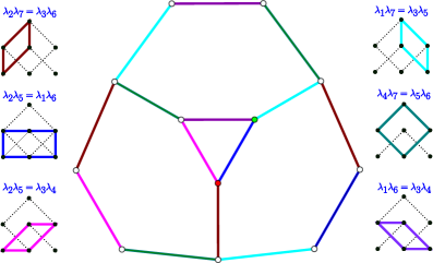
Figure 14: The permutohedra graph for $5_{2}$ knot consists of three $\Pi_{3}$ (shown schematically in bottom together with the formulas they correspond to) glued along common edges. The edges in this graph correspond to 6 types of transpositions arising from various quadruples of homology generators, which are also shown in various colors on the homological diagrams.

Following the above analysis we find that the permutohedra graph for $5_{2}$ has the structure shown in figure 14. The permutohedron arising from 6 permutations associated to $(0,1)$-splitting of the prequiver (91) lies on the top of the graph. The bottom-right $\Pi_{3}$ comes from all possible $(0,2)$-splittings of the prequiver (101). Finally, $(1,3)$-splittings of (104) lead to the bottom-left hexagon. The quiver (92) (or its reordered form (102)) is denoted by the green dot. The red dot represents the quiver (103) (or its reordered form (105)) found in KRSS1707long . The symmetry connecting these two quivers is denoted by the blue edge. Moreover, we find that each pair of permutohedra $\Pi_{3}$ identified above has 2 common quivers, which are connected by a transposition that is also common to such two permutohedra. Altogether, the permutohedra graph takes form of 3 permutohedra $\Pi_{3}$ glued along their edges, as shown in figure 14. The triangle in the middle of the graph represents two transpositions whose composition is also a transposition (not a 3-cycle), so it does not contradict the argument in section 3.1. In the figure we also show how various symmetries (transpositions of matrix elements that relate various equivalent quivers, which correspond to edges of the permutohedra graph) arise from quadruples of homology generators, and denote them in various colors. According to conjecture 5, we expect that figure 14 presents the whole equivalence class of quivers.

5.5 $7_{1}$ knot

Another interesting example is $7_{1}$ knot. Applying theorem 6 systematically, we find 13 equivalent quivers, which we list explicitly in the appendix A. More detailed analysis reveals that they form two permuthohedra $\Pi_{3}$ that share one common vertex (corresponding to a common quiver), and each of these $\Pi_{3}$ in addition shares a common vertex with one of the two permutohedra $\Pi_{2}$.

The generating function of colored superpolynomials takes the form FGSS1209 ; AFGS1203

$$P_{7_{1}}(x,a,q,t)=\sum_{r=0}^{\infty}\frac{x^{r}a^{6r}q^{-6r}}{(q^{2};q^{2})_{r}}\sum_{0\leq k_{3}\leq k_{2}\leq k_{1}\leq r}\left[\begin{array}[]{c}r\\ k_{1}\end{array}\right]\left[\begin{array}[]{c}k_{1}\\ k_{2}\end{array}\right]\left[\begin{array}[]{c}k_{2}\\ k_{3}\end{array}\right](-a^{2}q^{-2}t;q^{2})_{k_{1}}$$ (112)

$$\times\,q^{2[(2r+1)(k_{1}+k_{2}+k_{3})-rk_{1}-k_{1}k_{2}-k_{2}k_{3}]}t^{2(k_{1}+k_{2}+k_{3})}.$$

For $r=1$ we get the uncolored superpolynomial $P_{1}(a,q,t)=a^{6}q^{-6}+a^{6}q^{-2}t^{2}+a^{8}q^{-4}t^{3}+a^{6}q^{2}t^{4}+a^{8}t^{5}+a^{6}q^{6}t^{6}+a^{8}q^{4}t^{7}$. The corresponding homological diagram consists of one zig-zag made of 7 nodes, see figure 15.

Figure 15: Homology diagram for $7_{1}$ knot; labels $\lambda_{i}$ are consistent with (114).

First, we rewrite (112) as follows:

$$\begin{split}P_{7_{1}}(x,a,q,t)&=\sum_{\boldsymbol{\check{d}}}(-q)^{\boldsymbol{\check{d}}\cdot\check{C}\cdot\boldsymbol{\check{d}}}\frac{\boldsymbol{\check{x}}^{\boldsymbol{\check{d}}}}{(q^{2};q^{2})_{\boldsymbol{\check{d}}}}(-a^{2}q^{-2}t;q^{2})_{\check{d}_{2}+\check{d}_{3}+\check{d}_{4}}\Big{|}_{\boldsymbol{\check{x}}=x\boldsymbol{\check{\lambda}}}\\ \check{C}&=\left[\begin{array}[]{c:c:c:c}0&1&3&5\\ \hdashline 1&2&3&5\\ \hdashline 3&3&4&5\\ \hdashline 5&5&5&6\end{array}\right],\qquad\qquad\boldsymbol{\check{\lambda}}=\left[\begin{array}[]{c}a^{6}q^{-6}\\ a^{6}q^{-4}(-t)^{2}\\ a^{6}q^{-2}(-t)^{4}\\ a^{6}(-t)^{6}\end{array}\right].\end{split}$$ (113)

The (0,1)-splitting of the last three nodes with trivial permutation, $h_{1}=0$, and $\kappa=-a^{2}q^{-3}t$ leads to

$$C=\left[\begin{array}[]{c:cc:cc:cc}0&1&1&3&3&5&5\\ \hdashline 1&2&2&3&3&5&5\\ 1&2&3&4&4&6&6\\ \hdashline 3&3&4&4&4&5&5\\ 3&3&4&4&5&6&6\\ \hdashline 5&5&6&5&6&6&6\\ 5&5&6&5&6&6&7\\ \end{array}\right],\qquad\boldsymbol{\lambda}=\left[\begin{array}[]{c}a^{6}q^{-6}\\ a^{6}q^{-4}(-t)^{2}\\ a^{8}q^{-7}(-t)^{3}\\ a^{6}q^{-2}(-t)^{4}\\ a^{8}q^{-5}(-t)^{5}\\ a^{6}(-t)^{6}\\ a^{8}q^{-3}(-t)^{7}\end{array}\right],$$ (114)

which reproduces the quiver from KRSS1707long . More generally, splitting these three nodes with all possible permutations yields one permutohedron $\Pi_{3}$.

Furthermore, we can also rewrite (112) as

$$\begin{split}P_{7_{1}}(x,a,q,t)&=\sum_{\boldsymbol{\check{d}}}(-q)^{\boldsymbol{\check{d}}\cdot\check{C}\cdot\boldsymbol{\check{d}}}\frac{\boldsymbol{\check{x}}^{\boldsymbol{\check{d}}}}{(q^{2};q^{2})_{\boldsymbol{\check{d}}}}(-a^{2}q^{2r}t^{3};q^{2})_{\check{d}_{2}+\check{d}_{3}+\check{d}_{4}}\Big{|}_{\boldsymbol{\check{x}}=x\boldsymbol{\check{\lambda}}}\\ \check{C}&=\left[\begin{array}[]{c:c:c:c}6&5&5&5\\ \hdashline 5&0&1&3\\ \hdashline 5&1&2&3\\ \hdashline 5&3&3&4\end{array}\right],\qquad\qquad\boldsymbol{\check{\lambda}}=\left[\begin{array}[]{c}a^{6}(-t)^{6}\\ a^{6}q^{-6}\\ a^{6}q^{-4}(-t)^{2}\\ a^{6}q^{-2}(-t)^{4}\end{array}\right].\end{split}$$ (115)

In this case $(1,3)$-splitting of the last three nodes with permutation $\sigma=(2\ 4)$, $h_{1}=1$, and $\kappa=-a^{2}q^{-1}t^{3}$ gives a rearrangment of the quiver (114):

$$C=\left[\begin{array}[]{c:cc:cc:cc}6&5&6&5&6&5&6\\ \hdashline 5&0&1&1&3&3&5\\ 6&1&3&2&4&4&6\\ \hdashline 5&1&2&2&3&3&5\\ 6&3&4&3&5&4&6\\ \hdashline 5&3&4&3&4&4&5\\ 6&5&6&5&6&5&7\\ \end{array}\right],\qquad\boldsymbol{\lambda}=\left[\begin{array}[]{c}a^{6}(-t)^{6}\\ a^{6}q^{-6}\\ a^{8}q^{-7}(-t)^{3}\\ a^{6}q^{-4}(-t)^{2}\\ a^{8}q^{-5}(-t)^{5}\\ a^{6}q^{-2}(-t)^{4}\\ a^{8}q^{-3}(-t)^{7}\end{array}\right],$$ (116)

and analogous splittings with all other permutations give rise to another permutohedron $\Pi_{3}$. Therefore we have identified two permutohedra that share a common vertex, which represents the quiver matrix  (114) (or its reordered form (116)). Let us now focus on $\Pi_{3}$ arising from the prequiver (113). One can check that almost all quivers represented by its other vertices cannot be obtained from other prequivers. The only exception is

$$C=\left[\begin{array}[]{c:cc:cc:cc}0&1&1&3&3&5&5\\ \hdashline 1&2&2&3&4&5&6\\ 1&2&3&3&4&5&6\\ \hdashline 3&3&3&4&4&5&6\\ 3&4&4&4&5&5&6\\ \hdashline 5&5&5&5&5&6&6\\ 5&6&6&6&6&6&7\\ \end{array}\right],\qquad\boldsymbol{\lambda}=\left[\begin{array}[]{c}a^{6}q^{-6}\\ a^{6}q^{-4}(-t)^{2}\\ a^{8}q^{-7}(-t)^{3}\\ a^{6}q^{-2}(-t)^{4}\\ a^{8}q^{-5}(-t)^{5}\\ a^{6}(-t)^{6}\\ a^{8}q^{-3}(-t)^{7}\end{array}\right],$$ (117)

that arises from (0,1)-splitting of (113) with permutation $\sigma=(2\ 4)$. Indeed, $(0,1)$-splitting of the last two nodes of the prequiver

$$\check{C}=\left[\begin{array}[]{ccc:c:c}0&1&5&1&3\\ 1&2&6&2&4\\ 5&6&7&6&6\\ \hdashline 1&2&6&3&4\\ \hdashline 3&4&6&4&5\\ \end{array}\right],\qquad\qquad\boldsymbol{\check{\lambda}}=\left[\begin{array}[]{c}a^{6}q^{-6}\\ a^{6}q^{-4}(-t)^{2}\\ a^{8}q^{-3}(-t)^{7}\\ a^{8}q^{-7}(-t)^{3}\\ a^{8}q^{-5}(-t)^{5}\end{array}\right],$$ (118)

with permutation $\sigma=(4\ 5)$, $h_{1}=2,\,h_{2}=1,\,h_{3}=0$, and $\kappa=-a^{-2}q^{5}t$ leads to

$$C=\left[\begin{array}[]{ccc:cc:cc}0&1&5&1&3&3&5\\ 1&2&6&2&3&4&5\\ 5&6&7&6&6&6&6\\ \hdashline 1&2&6&3&3&4&5\\ 3&3&6&3&4&4&5\\ \hdashline 3&4&6&4&4&5&5\\ 5&5&6&5&5&5&6\\ \end{array}\right],\qquad\qquad\boldsymbol{\lambda}=\left[\begin{array}[]{c}a^{6}q^{-6}\\ a^{6}q^{-4}(-t)^{2}\\ a^{8}q^{-3}(-t)^{7}\\ a^{8}q^{-7}(-t)^{3}\\ a^{6}q^{-2}(-t)^{4}\\ a^{8}q^{-5}(-t)^{5}\\ a^{6}q^{-6}\end{array}\right],$$ (119)

which is a rearrangement of (117). This means that the quiver (117) (or its reordered form (119)) is a gluing point of permutohedra $\Pi_{3}$ and $\Pi_{2}$.

Figure 16: The permutohedra graph for $7_{1}$ knot consists of two $\Pi_{3}$ and two $\Pi_{2}$ appropriately glued. Altogether it has 13 vertices representing equivalent quivers, and 8 symmetries corresponding to various quadruples of homology generators (and represented by different colors of the edges in the graph).

An analogous phenomenon occurs for the second $\Pi_{3}$, which is also connected to another permutohedron $\Pi_{2}$. Altogether, the permutohedra graph consists of two $\Pi_{3}$ and two $\Pi_{2}$, as shown in figure 16. The quiver (114) (or equivalently (116)), also found in KRSS1707long , is common to the two $\Pi_{3}$ and it is represented by the red dot. The $\Pi_{3}$ on the left arises from the prequiver (113), whereas the one on the right corresponds to the prequiver (115). The quiver (117) (or its reordered form (119)) is represented by the green node, and it glues the left $\Pi_{3}$ with $\Pi_{2}$ coming from the prequiver (118). Analogous gluing point is present on the right-hand side of the graph. In total we found 8 non-trivial symmetries shown in figure 16 in various colors, and 13 equivalent quivers that we list explicitly in the appendix A. Using the procedure described in section 3.1 we checked that there are no other equivalent quivers. According to conjecture 5, we expect that figure 16 presents the whole equivalence class of quivers.

5.6 $6_{1}$ knot

Another example that we consider is $6_{1}$ knot. We have found 141 equivalent quivers, which form quite complicated permutohedra graph, shown in figure 17. These quivers are related to each other by 16 symmetries (transpositions of various pairs of quiver matrices).

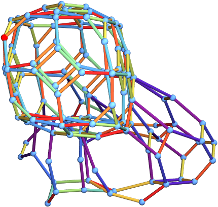
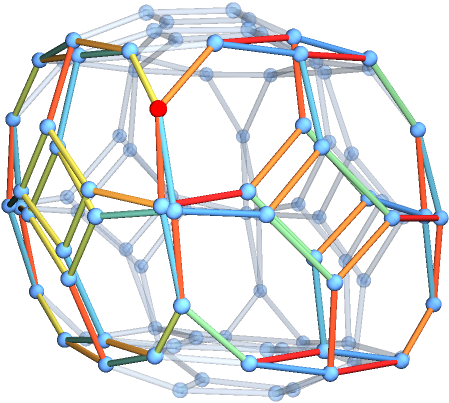
Figure 17: The permutohedra graph for $6_{1}$ knot has 141 vertices that represent equivalent quivers (left). Excluding symmetries that involve $\lambda_{1}$ reduces the whole graph to a cube-like shape (right). Each face of this cube is one $\Pi_{4}$ (a bit squashed), and neighboring $\Pi_{4}$’s are glued along a square, which is a common face to both $\Pi_{4}$’s. The red vertex represents the quiver (127) (or its reordered form (129)).

The generating function of colored superpolynomials for $6_{1}$ knot reads FGSS1209 :

$$P_{6_{1}}(x,a,q,t)=\sum_{r=0}^{\infty}\frac{x^{r}}{(q^{2};q^{2})_{r}}\sum_{0\leq k_{2}\leq k_{1}\leq r} \left[\begin{array}[]{c}r\\ k_{1}\end{array}\right]\left[\begin{array}[]{c}k_{1}\\ k_{2}\end{array}\right](-a^{-2}q^{2}t^{-1};q^{-2})_{k_{1}}(-a^{-2}q^{-2r}t^{-3};q^{-2})_{k_{1}}$$ (124)

$$\times a^{2(k_{1}+k_{2})}t^{2(k_{1}+k_{2})}q^{2(k_{1}^{2}+k_{2}^{2}-k_{1}-k_{2})}.$$ (125)

Linear order of this equation gives the uncolored superpolynomial $P_{1}(a,q,t)=1+a^{-2}t^{-2}+q^{2}t+q^{-2}t^{-1}+a^{2}t^{2}+1+a^{2}q^{2}t^{3}+a^{2}q^{-2}t+a^{4}t^{4}$. The corresponding homological diagram, shown in figure 18, consists of 2 diamonds and a degenerate zig-zag made of one node that coincides with one vertex of the upper diamond, so that $\lambda_{1}=\lambda_{6}$ .

Figure 18: Homology diagram for $6_{1}$ knot; labels $\lambda_{i}$ are consistent with (127).

First, we rewrite (124) as

$$\begin{split}P_{6_{1}}(x,a,q,t)&=\sum_{\boldsymbol{\check{d}}}(-q)^{\boldsymbol{\check{d}}\cdot\check{C}\cdot\boldsymbol{\check{d}}}\frac{\boldsymbol{\check{x}}^{\boldsymbol{\check{d}}}}{(q^{2};q^{2})_{\boldsymbol{\check{d}}}}(-a^{2}q^{-2}t;q^{2})_{\check{d}_{2}+\check{d}_{3}+\check{d}_{4}+\check{d}_{5}}\Big{|}_{\boldsymbol{\check{x}}=x\boldsymbol{\check{\lambda}}}\\ \check{C}&=\left[\begin{array}[]{c:c:c:c:c}0&-1&-1&-1&-1\\ \hdashline-1&-2&-2&-2&-1\\ \hdashline-1&-2&-1&-2&-1\\ \hdashline-1&-2&-2&0&0\\ \hdashline-1&-1&-1&0&1\end{array}\right],\phantom{\qquad}\phantom{\qquad}\boldsymbol{\check{\lambda}}=\left[\begin{array}[]{c}1\\ a^{-2}q^{2}(-t)^{-2}\\ q^{-1}(-t)^{-1}\\ 1\\ a^{2}q^{-3}(-t)\\ \end{array}\right].\end{split}$$ (126)

Then $(1,3)$-splitting of the last four nodes with permuation $\sigma=(2\ 4\ 5\ 3)$, $h_{1}=1$, and $\kappa=-a^{2}q^{-1}t^{3}$ leads to the quiver found in KRSS1707long :

$$C=\left[\begin{array}[]{c:cc:cc:cc:cc}0&-1&0&-1&0&-1&0&-1&0\\ \hdashline-1&-2&-1&-2&-1&-2&0&-1&0\\ 0&-1&1&0&1&-1&1&1&2\\ \hdashline-1&-2&0&-1&0&-2&0&-1&1\\ 0&-1&1&0&2&-1&1&0&2\\ \hdashline-1&-2&-1&-2&-1&0&1&0&1\\ 0&0&1&0&1&1&3&2&3\\ \hdashline-1&-1&1&-1&0&0&2&1&2\\ 0&0&2&1&2&1&3&2&4\end{array}\right],\phantom{\qquad}\phantom{\qquad}\boldsymbol{\lambda}=\left[\begin{array}[]{c}1\\ a^{-2}q^{2}(-t)^{-2}\\ q(-t)\\ q^{-1}(-t)^{-1}\\ a^{2}q^{-2}(-t)^{2}\\ 1\\ a^{2}q^{-1}(-t)^{3}\\ a^{2}q^{-3}(-t)\\ a^{4}q^{-4}(-t)^{4}\end{array}\right].$$ (127)

On the other hand, we can rewrite (124) in the form

$$\begin{split}P_{6_{1}}(x,a,q,t)&=\sum_{\boldsymbol{\check{d}}}(-q)^{\boldsymbol{\check{d}}\cdot\check{C}\cdot\boldsymbol{\check{d}}}\frac{\boldsymbol{\check{x}}^{\boldsymbol{\check{d}}}}{(q^{2};q^{2})_{\boldsymbol{\check{d}}}}\Pi_{\check{d}_{2},\check{d}_{3},\check{d}_{4},\check{d}_{5}}\Big{|}_{\boldsymbol{\check{x}}=x\boldsymbol{\check{\lambda}}}\\ \Pi_{\check{d}_{2},\check{d}_{3},\check{d}_{4},\check{d}_{5}}&=\sum\limits_{\alpha_{2}+\beta_{2}=\check{d}_{2}}\sum\limits_{\alpha_{3}+\beta_{3}=\check{d}_{3}}\sum\limits_{\alpha_{4}+\beta_{4}=\check{d}_{4}}\sum\limits_{\alpha_{5}+\beta_{5}=\check{d}_{5}}\prod_{i=2}^{5}\frac{(a^{2}q^{-2}t^{2})^{\beta_{i}}(q^{2};q^{2})_{\check{d}_{i}}}{(q^{2};q^{2})_{\alpha_{i}}(q^{2};q^{2})_{\beta_{i}}}\\ &\times(-q)^{2(\beta_{2}+\beta_{3}+\beta_{4}+\beta_{5})^{2}+2(\alpha_{2}\beta_{3}+\alpha_{2}\beta_{4}+\alpha_{2}\beta_{5}+\alpha_{3}\beta_{4}+\alpha_{3}\beta_{5}+\alpha_{4}\beta_{5})}\\ \check{C}&=\left[\begin{array}[]{c:c:c:c:c}0&-1&-1&0&0\\ \hdashline-1&-2&-2&-1&-1\\ \hdashline-1&-2&-1&0&0\\ \hdashline 0&-1&0&1&1\\ \hdashline 0&-1&0&1&2\end{array}\right],\phantom{\qquad}\phantom{\qquad}\boldsymbol{\check{\lambda}}=\left[\begin{array}[]{c}1\\ a^{-2}q^{2}(-t)^{-2}\\ q^{-1}(-t)^{-1}\\ q(-t)\\ a^{2}q^{-2}(-t)^{2}\\ \end{array}\right],\end{split}$$ (128)

Then, $(0,2)$-splitting of the last four nodes with permutation $\sigma=(2\ 5)(3\ 4)$, $h_{1}=0$, and $\kappa=a^{2}q^{-2}t^{2}$ leads to

$$C=\left[\begin{array}[]{c:cc:cc:cc:cc}0&-1&-1&-1&-1&0&0&0&0\\ \hdashline-1&-2&-2&-2&-1&-1&0&-1&0\\ -1&-2&0&-2&0&-1&1&-1&1\\ \hdashline-1&-2&-2&-1&-1&0&1&0&1\\ -1&-1&0&-1&1&0&2&0&2\\ \hdashline 0&-1&-1&0&0&1&1&1&2\\ 0&0&1&1&2&1&3&1&3\\ \hdashline 0&-1&-1&0&0&1&1&2&2\\ 0&0&1&1&2&2&3&2&4\end{array}\right],\phantom{\qquad}\phantom{\qquad}\boldsymbol{\lambda}=\left[\begin{array}[]{c}1\\ a^{-2}q^{2}(-t)^{-2}\\ 1\\ q^{-1}(-t)^{-1}\\ a^{2}q^{-3}(-t)\\ q(-t)\\ a^{2}q^{-1}(-t)^{3}\\ a^{2}q^{-2}(-t)^{2}\\ a^{4}q^{-4}(-t)^{4}\end{array}\right].$$ (129)

which is a rearrangement of (127). This means that the above quiver is common to two permutohedra $\Pi_{4}$, and it is represented by the red dot in figure 17 and 19. In figure 19, which shows a planar projection of a part of the permutohedra graph, $\Pi_{4}$ coming from the prequiver (126) is oriented along axis $\nearrow$, whereas $\Pi_{4}$ oriented along $\nwarrow$ corresponds to the prequiver (128). All other quiver matrices that we found are listed in the Mathematica file attached to the arXiv submission. According to conjecture 5, we expect that there are no more equivalent quivers and figure 19 presents the whole equivalence class.

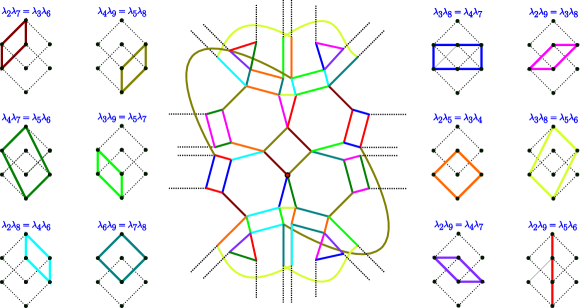
Figure 19: Planar projection of a part of the permutohedra graph for $6_{1}$ knot. In homological diagrams (on left and right) it is indicated how some of its symmetries, corresponding to edges of the graph, arise from quadruples of homology generators. The positions of two two permutohedra $\Pi_{4}$ mentioned in the text are indicated schematically in the bottom.

5.7 $(2,2p+1)$ torus knots

The last example we consider is a series of $(2,2p+1)$ torus knots. For this class the number of equivalent quivers grows rapidly; for $p=1,...,7$ we have found respectively 1, 3, 13, 68, 405, 2684 and 19557 equivalent quivers, which permutohedra graphs have an interesting structure. For $p=1$ there is just one corresponding quiver, see section 5.1; for $p>1$ the permutohedra graph consists of two series of larger and larger permutohedra $\Pi_{2},\ldots,\Pi_{p}$ (and several additional permutohedra of small size that do not belong to these series). In each of these two series each permutohedron $\Pi_{i}$ is connected to $\Pi_{i-1}$ and $\Pi_{i+1}$ (for $i=3,\ldots,p-1$), and the two largest permutohedra $\Pi_{p}$ from both series are also connected. Such a structure is present for $5_{1}$, $7_{1}$, $9_{1}$ and $11_{1}$ knots in figures 12, 16, 2, and 3, respectively. In this section we explain how two largest permutohedra $\Pi_{p}$ for $(2,2p+1)$ torus knot arise.

To start with, note that the generating function of superpolynomials for $(2,2p+1)$-torus knot can be written, among others, in the following two equivalent ways, which correspond to different grading conventions for the $S^{r}$-colored HOMFLY-PT homologies AFGS1203 ; FGSS1209 :

$$P_{T_{2,2p+1}}(x,a,q,t) =\sum_{r\geq 0}x^{r}a^{2pr}q^{-2pr}\sum_{0\leq k_{p}\leq\ldots\leq k_{2}\leq k_{1}\leq r}\left[\begin{array}[]{c}r\\ k_{1}\end{array}\right]\left[\begin{array}[]{c}k_{1}\\ k_{2}\end{array}\right]\cdots\left[\begin{array}[]{c}k_{p-1}\\ k_{p}\end{array}\right]$$ (136)

$$\quad\times q^{2\sum_{i=1}^{p}((2r+1)k_{i}-k_{i-1}k_{i})}t^{2(k_{1}+k_{2}+\ldots+k_{p})}(-a^{2}q^{-2}t;q^{2})_{k_{1}}=$$

$$=\sum_{r\geq 0}x^{r}a^{2pr}q^{-2pr}\sum_{0\leq k_{p}\leq\ldots\leq k_{2}\leq k_{1}\leq r}\left[\begin{array}[]{c}r\\ k_{1}\end{array}\right]\left[\begin{array}[]{c}k_{1}\\ k_{2}\end{array}\right]\cdots\left[\begin{array}[]{c}k_{p-1}\\ k_{p}\end{array}\right]$$ (143)

$$\quad\times q^{2\sum_{i=1}^{p}((2r+1)k_{i}-k_{i-1}k_{i})}t^{2(k_{1}+k_{2}+\ldots+k_{p})}(-a^{2}q^{2r}t^{3};q^{2})_{r-k_{p}}.$$

For $p=1$, i.e. $3_{1}$ knot, the above expressions reduce to

$$\begin{split}\sum_{0\leq k_{1}\leq r}\left[\begin{array}[]{c}r\\ k_{1}\end{array}\right]\left[\begin{array}[]{c}k_{1}\\ k_{2}\end{array}\right]q^{2k_{1}(r+1)}t^{2k_{1}}&(-a^{2}q^{-2}t;q^{2})_{k_{1}}\\ &=\sum_{0\leq k_{1}\leq r}\left[\begin{array}[]{c}r\\ k_{1}\end{array}\right]\left[\begin{array}[]{c}k_{1}\\ k_{2}\end{array}\right]q^{2k_{1}(r+1)}t^{2k_{1}}(-a^{2}q^{2r}t^{3};q^{2})_{r-k_{1}},\end{split}$$ (144)

and the two permutohedra consist of one vertex. They are in fact identified, so that the full permutohedra graph consists just of one $\Pi_{1}$. In general, both (136) and (143) can be rewritten in form (44) using the formula

$$\left[\begin{array}[]{c}r\\ k_{1}\end{array}\right]\left[\begin{array}[]{c}k_{1}\\ k_{2}\end{array}\right]\cdots\left[\begin{array}[]{c}k_{p-1}\\ k_{p}\end{array}\right]=\frac{(q^{2};q^{2})_{r}}{(q^{2};q^{2})_{r-k_{1}}(q^{2};q^{2})_{k_{1}-k_{2}}\cdots(q^{2};q^{2})_{k_{p-1}-k_{p}}(q^{2};q^{2})_{k_{p}}}.$$ (145)

In case of (136) we set

$$\check{d}_{1} =r-k_{1}, \check{d}_{2} =k_{1}-k_{2}, \check{d}_{3} =k_{2}-k_{3}, \check{d}_{4} =k_{3}-k_{4},$$

$$\ldots \check{d}_{i+1} =k_{i}-k_{i+1}, \ldots \check{d}_{p+1} =k_{p},$$

which leads to

$$P_{T_{2,2p+1}}(x,a,q,t)=\sum_{\boldsymbol{\check{d}}}(-q)^{\boldsymbol{\check{d}}\cdot\check{C}\cdot\boldsymbol{\check{d}}}\frac{\boldsymbol{\check{x}}^{\boldsymbol{\check{d}}}}{(q^{2};q^{2})_{\boldsymbol{\check{d}}}}(-a^{2}q^{-2}t;q^{2})_{\check{d}_{2}+\dots+\check{d}_{p+1}}\Big{|}_{\boldsymbol{\check{x}}=x\boldsymbol{\check{\lambda}}}$$ (146)

$$\check{C}=\left[\begin{array}[]{c:c:c:c:c:c:c}0&1&3&5&\dots&2p-3&2p-1\\ \hdashline 1&2&3&5&\dots&2p-3&2p-1\\ \hdashline 3&3&4&5&\dots&2p-3&2p-1\\ \hdashline 5&5&5&6&\dots&2p-3&2p-1\\ \hdashline\vdots&\vdots&\vdots&\vdots&\ddots&\vdots&\vdots\\ \hdashline 2p-3&2p-3&2p-3&2p-3&\dots&2p-2&2p-1\\ \hdashline 2p-1&2p-1&2p-1&2p-1&\dots&2p-1&2p\\ \end{array}\right]\left.\begin{array}[]{c}\check{d}_{1}\\ \check{d}_{2}\\ \check{d}_{3}\\ \check{d}_{4}\\ \vdots\\ \check{d}_{p}\\ \check{d}_{p+1}\end{array}\right.,\quad\boldsymbol{\check{\lambda}}=\left[\begin{array}[]{c}a^{2p}q^{-2p}\\ a^{2p}q^{-2(p-1)}(-t)^{2}\\ a^{2p}q^{-2(p-2)}(-t)^{4}\\ a^{2p}q^{-2(p-3)}(-t)^{6}\\ \vdots\\ a^{2p}q^{-2}(-t)^{2p+2}\\ a^{2p}(-t)^{2p}\end{array}\right].$$ (168)

The $(0,1)$-splitting of the nodes corresponding to $\check{d}_{2},\dots,\check{d}_{p+1}$ with trivial permutation, $h_{1}=0$, and $\kappa=\xi q^{-1}=-a^{2}q^{-3}t$ produces the quiver found in KRSS1707long :

$$C=\left[\begin{array}[]{c:cc:cc:c:cc}0&1&1&3&3&\dots&2p-1&2p-1\\ \hdashline 1&2&2&3&3&\dots&2p-1&2p-1\\ 1&2&3&4&4&\dots&2p&2p\\ \hdashline 3&3&4&4&4&\dots&2p-1&2p-1\\ 3&3&4&4&5&\dots&2p&2p\\ \hdashline\vdots&\vdots&\vdots&\vdots&\vdots&\ddots&\vdots&\vdots\\ \hdashline 2p-1&2p-1&2p&2p-1&2p&\dots&2p&2p\\ 2p-1&2p-1&2p&2p-1&2p&\dots&2p&2p+1\\ \end{array}\right],\quad\boldsymbol{\lambda}=\left[\begin{array}[]{c}a^{2p}q^{-2p}\\ a^{2p}q^{-2(p-1)}(-t)^{2}\\ a^{2(p+1)}q^{-2(p-1)-3}(-t)^{3}\\ a^{2p}q^{-2(p-2)}(-t)^{4}\\ a^{2(p+1)}q^{-2(p-2)-3}(-t)^{5}\\ \vdots\\ a^{2p}(-t)^{2p}\\ a^{2(p+1)}q^{-3}(-t)^{2p+1}\end{array}\right].$$ (169)

On the other hand, for the expression (143) we introduce

$$\check{d}_{1} =r-(r-k_{p})=k_{p},$$

$$\check{d}_{2} =r-k_{1}, \check{d}_{3} =k_{1}-k_{2}, \ldots \check{d}_{p+1} =k_{p-1}-k_{p},$$

and then find

$$P_{T_{2,2p+1}}(x,a,q,t)=\sum_{\boldsymbol{\check{d}}}(-q)^{\boldsymbol{\check{d}}\cdot\check{C}\cdot\boldsymbol{\check{d}}}\frac{\boldsymbol{\check{x}}^{\boldsymbol{\check{d}}}}{(q^{2};q^{2})_{\boldsymbol{\check{d}}}}(-a^{2}q^{2r}t^{3};q^{2})_{\check{d}_{2}+\dots+\check{d}_{p+1}}\Big{|}_{\boldsymbol{\check{x}}=x\boldsymbol{\check{\lambda}}}$$ (170)

$$\check{C}=\left[\begin{array}[]{c:c:c:c:c:c:c}2p&2p-1&2p-1&2p-1&\dots&2p-1&2p-1\\ \hdashline 2p-1&0&1&3&\dots&2p-5&2p-3\\ \hdashline 2p-1&1&2&3&\dots&2p-5&2p-3\\ \hdashline 2p-1&3&3&4&\dots&2p-5&2p-3\\ \hdashline\vdots&\vdots&\vdots&\vdots&\ddots&\vdots&\vdots\\ \hdashline 2p-1&2p-5&2p-5&2p-5&\dots&2p-4&2p-3\\ \hdashline 2p-1&2p-3&2p-3&2p-3&\dots&2p-3&2p-2\\ \end{array}\right]\left.\begin{array}[]{c}\check{d}_{1}\\ \check{d}_{2}\\ \check{d}_{3}\\ \check{d}_{4}\\ \vdots\\ \check{d}_{p}\\ \check{d}_{p+1}\end{array}\right.,\ \boldsymbol{\check{\lambda}}=\left[\begin{array}[]{c}a^{2p}(-t)^{2p}\\ a^{2p}q^{-2p}\\ a^{2p}q^{-2(p-1)}(-t)^{2}\\ a^{2p}q^{-2(p-2)}(-t)^{4}\\ \vdots\\ a^{2p}q^{-4}(-t)^{2p-4}\\ a^{2p}q^{-2}(-t)^{2p-2}\end{array}\right].$$ (192)

One can check that the $(1,3)$-splitting of the nodes corresponding to $\check{d}_{2},\dots,\check{d}_{p+1}$ with permutation $\sigma=(2\ \ (p+1))$, $h_{1}=1$, and $\kappa=-a^{2}q^{-1}t^{3}$ yields the same quiver as in (169).

Note that both prequivers given above are the same up to reordering of nodes, however the two splittings are different. This is why we obtain two different permutohedra $\Pi_{p}$, respectively left (for (136)) and right ((143)) in figures 2, 3, 12, and  16. These two permutohedra share the quiver matrix (169), which can be obtained from appropriate splittings of corresponding prequivers, as explained above. An interested reader may conduct careful analysis of other permutohedra in these graphs.

6 Examples – local structure

In the previous section we presented permutohedra graphs for simple knots and discussed in detail the structure of glued permutohedra embedded in these graphs. In this section we take the opposite perspective and study the local structure: we choose some particular quiver and identify all equivalent quivers related to it by a single transposition of matrix elements (a single symmetry, to which we refer as local). We also provide interpretation of such equivalences in terms of homological diagrams. We conduct such an analysis for infinite families of $(2,2p+1)$ torus knots (also denoted $T_{2,2p+1}$), $TK_{2|p|+2}$ and $TK_{2p+1}$ twist knots, and in addition $6_{2},6_{3}$ and $7_{3}$ knots. The quivers that we analyze are those found in KRSS1707long (apart from the quiver for $7_{3}$ knot that was found in SW1711 ), and they are indicated by red vertices in permutohedra graphs in figures  11, 12, 14, and 19. The symmetries that we analyze in this section are represented by edges adjacent to these red vertices.

Recall that:

• Quiver matrices for $(2,2p+1)$ torus knots that we consider are given in (169). A homological diagram for $(2,2p+1)$ torus knot consists of one zig-zag made of $2p+1$ generators.

• Quiver matrices for twist knots $TK_{2|p|+2}$ (i.e. $4_{1},6_{1},8_{1},\dots$ knots) are given in the appendix B. A homological diagram for $TK_{2|p|+2}$ knot consists of $p$ diamonds and a zig-zag made of one generator, so altogether it has $4p+1$ generators.

• Quiver matrices for twist knots $TK_{2p+1}$ (i.e. $3_{1},5_{2},7_{2},\dots$ knots) are also given in the appendix B. A homological diagram for $TK_{2p+1}$ knot consists of $p-1$ diamonds and a zig-zag of length 3, so altogether it has $4p-1$ generators.

Figure 20: Enumeration of wedges and diamonds in the homology diagrams, from left to right: $T_{2,2p+1}$, $TK_{2|p|+2}$, $TK_{2p+1}$.

In this section we fix the ordering of homological generators (and correspondingly quiver nodes) as shown in figure 20. In what follows we call a part of a zig-zag consisting of three consecutive nodes that form a shape $\wedge$ a wedge. We enumerate diamonds and wedges by $r,r^{\prime},r^{\prime\prime},r^{\prime\prime\prime},\dots$, such that $r\leq r^{\prime}\leq r^{\prime\prime}\leq r^{\prime\prime\prime}\dots$; for a wedge or a zig-zag labeled by $r$, we enumerate the generators it consists of as in the bottom of figure 20. We write pairings $\lambda_{a}\lambda_{b}=\lambda_{c}\lambda_{d}$ as column vectors with entries $a,b,c,d$. Recall that we call such a paring a symmetry if quiver matrices with elements $C_{ab}$ and $C_{cd}$ exchanged are equivalent. We also call the requirements $C_{ai}+C_{bi}=C_{ci}+C_{di}$ (for $i\neq a,b,c,d$) spectator constraints.

Theorem 9.

For infinite families of knots $T_{2,2p+1},TK_{2|p|+2},TK_{2p+1},p=1,2,3,\dots$, quiver matrices given respectively in (169) and in appendix B, have the following local symmetries:

$$T_{2,2p+1}: \ \begin{bmatrix}2r\\ 2r^{\prime}+3\\ 2r+3\\ 2r^{\prime}\end{bmatrix},\ \begin{bmatrix}2r+3\\ 2r^{\prime}+2\\ 2r+2\\ 2r^{\prime}+3\end{bmatrix}$$ (193)

$$TK_{2|p|+2}: \ \begin{bmatrix}4r-1\\ 4r^{\prime}\\ 4r\\ 4r^{\prime}-1\end{bmatrix},\ \begin{bmatrix}4r-1\\ 4r^{\prime}-2\\ 4r-2\\ 4r^{\prime}-1\end{bmatrix},\ \begin{bmatrix}4r+1\\ 4r^{\prime}\\ 4r\\ 4r^{\prime}+1\end{bmatrix},\ \begin{bmatrix}4r+1\\ 4r^{\prime\prime}-2\\ 4r^{\prime}+1\\ 4r^{\prime}-2\end{bmatrix},\ \begin{bmatrix}4\\ 4p-1\\ 5\\ 4p-2\end{bmatrix}$$

$$TK_{2p+1}: \ \begin{bmatrix}2\\ 4r^{\prime}+3\\ 3\\ 4r^{\prime}+2\end{bmatrix},\ \begin{bmatrix}2\\ 4r^{\prime}+1\\ 1\\ 4r^{\prime}+2\end{bmatrix},\ \begin{bmatrix}2\\ 4p+1\\ 3\\ 4p\end{bmatrix}\bigcup\mathcal{T}\left(TK_{2|p|+2}\setminus\begin{bmatrix}4\\ 4p-1\\ 5\\ 4p-2\end{bmatrix}\right)$$

where $r^{\prime}=r+1$, $r^{\prime\prime}=r+2$, and

$$\mathcal{T}\left(TK_{2|p|+2}\setminus\begin{bmatrix}4\\ 4p-1\\ 5\\ 4p-2\end{bmatrix}\right):=\begin{bmatrix}4r+2\\ 4r^{\prime}+1\\ 4r+1\\ 4r^{\prime}+2\end{bmatrix},\ \begin{bmatrix}4r\\ 4r^{\prime}+1\\ 4r+1\\ 4r^{\prime}\end{bmatrix},\ \begin{bmatrix}4r+2\\ 4r^{\prime}+3\\ 4r+3\\ 4r^{\prime}+2\end{bmatrix},\ \begin{bmatrix}4r\\ 4r^{\prime\prime}+3\\ 4r^{\prime}\\ 4r^{\prime}+3\end{bmatrix}.$$ (194)

Figure 21: The local symmetries for $T_{2,2p+1}$ torus knots, $r=0,\dots,p-1$ (the symmetry exists only for $r^{\prime}=r+1$)

Figure 22: The local symmetries for twist knots. The symmetries which are shared between $TK_{2|p|+2}$ and $TK_{2p+1}$ twist knots do not have blue labels (any choice of $\lambda$’s ordering from figure 20 is valid for them). The top-right symmetry is signature for the $TK_{2|p|+2}$ twist knots, whereas the three bottom ones – for $TK_{2p+1}$ twist knots.

Recall again that entries of the vectors given above are labels of appropriate quadruples of quiver nodes or homology generators. For $(2,2p+1)$ torus knots, the condition $r^{\prime}=r+1$ means that these generators belong to two consecutive wedges, see figure 21. For twist knots, generators that encode a symmetry belong to various diamonds or the wedge, see figure 22. Below we give a proof of theorem 9 divided into three parts, each corresponding to one of the infinite families of knots. It is followed by the analysis of $6_{2},6_{3},7_{3}$ knots.

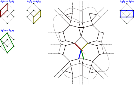
Figure 23: The four local symmetries of quiver (124) corresponding to $6_{1}$ knot, shown as the colorful thick edges

6.1 $(2,2p+1)$ torus knots

Figure 24: Homology diagram for $(2,2p+1)$ torus knot and labeling of its generators (the labeling of wedges is shown in figure 20).

For this family of knots, the homology diagram is a chain of $p$ wedges joined together. The wedges are labeled by $r=0,1,2,\dots,p-1$ as in figure 20, and the labeling of all generators is shown explicitly in figure 24. Note that what we label as the zeroth node corresponds to the quiver series parameter $x_{1}$, while the $i$-th node for $i>1$ corresponds to $x_{i}$. This notation is convenient, since in the formulas we can let $r=0$ referring to the first wedge, so we do not have to treat it separately. If $r$ and $r^{\prime}$ label two wedges and $r^{\prime}=r+1$, they share the common node labeled by $2r+2=2r^{\prime}$.

Note that the quiver matrix (169) (its special cases are given in (61, 81, 114)) has elements $C_{ij}$ such that

$$i,j \ C_{ij}=j-1, i=j: \ C_{jj}=j,$$ both odd or even: (195)

$$i j \ C_{ij}=j, j \ C_{1j}=j-1,$$ odd, even: even:

$$i j \ C_{ij}=j-2+\delta_{i+1,j},\qquad j \ C_{1j}=j-2.$$ even, odd: odd:

Figure 25: Pairings between the two wedges: type 2A.1 (left) and 2A.2 (right)

.

We now use theorem 6 to determine symmetries of this quiver. First, suppose that a pairing is made of generators from only two wedges, which are located in a generic position and not necessarily joined together, see figure 25. A direct check of conditions from theorem 6 shows that the two pairings in figure 25 are the symmetries if $r^{\prime}=r+1$, see figure 27. In order to confirm that there are no other symmetries, we label the four wedges by $r,r^{\prime},r^{\prime\prime},r^{\prime\prime\prime}$ such that $r<r^{\prime}<r^{\prime\prime}<r^{\prime\prime\prime}$ (see figure 26).

Figure 26: Pairings between 3 and 4 wedges, which are not symmetries for the quiver matrix (169). From top to bottom: 3A.1, 3A.2, 4A.1, 4A.2.

In consequence equation (195) leads to the following pairings:

3A.1: $$\quad C_{ab}=2r^{\prime\prime}+1,\;C_{cd}=2r^{\prime}+1 \quad C_{ab}=2r^{\prime\prime}+2,\;C_{cd}=2r^{\prime}+1$$ 3A.2:

4A.1: $$\quad C_{ab}=2r^{\prime\prime\prime}+1,\;C_{cd}=\begin{cases}2r^{\prime}+1,\;r^{\prime\prime}=r^{\prime}+1\\ 2r^{\prime\prime},\;r^{\prime\prime}>r^{\prime}+1\end{cases} \quad C_{ab}=2r^{\prime\prime\prime}+2,\;C_{cd}=2r^{\prime\prime}+1$$ 4A.2:

It follows that the condition $|C_{ab}-C_{cd}|=1$ from theorem 6 cannot be met in all these cases, so the only symmetries are indeed those in figure 21.

Pairing $b=c+3,d=a+3$ $$\begin{aligned} a=&\ a~{}\\ b=&\ c+3\\ c=&\ c\\ d=&\ a+3\end{aligned}\qquad\begin{pmatrix}a&\boxed{b-2}&c-1&d-2\\ \boxed{b-2}&b&b-2&b-1\\ c-1&b-2&c&c\\ d-2&b-1&c&d\\ \end{pmatrix}$$ $\displaystyle s<a,\ \text{odd}$ $\displaystyle\ a~{}+(b-1)=c+(d-1)$ $\displaystyle s<a,\ \text{even}$ $\displaystyle\ (a-1)+(b-2)=$ $\displaystyle\ (c-1)+(d-2)$ $\displaystyle s>b,\ \text{odd}$ $\displaystyle\ (s-2)+(s-1)=$ $\displaystyle\ (s-2)+(s-1)$ $\displaystyle s>b,\ \text{even}$ $\displaystyle\ (s-1)+s=(s-1)+s$ $\displaystyle d<s<c,\ \text{odd}$ $\displaystyle\ (s-2)+(b-1)\neq c+(s-1)$ $\displaystyle d<s<c,\ \text{even}$ $\displaystyle\ (s-1)+(b-2)\neq(c-1)+d$ $\displaystyle s=a+2$ $\displaystyle\ (i+1)+(j-2)\neq$ $\displaystyle\ (k-1)+(l-1)$ $\displaystyle s=c+1$ $\displaystyle\ (s-2)+(j-1)\neq$ $\displaystyle\ (s-1)+(s-1)$ Pairing $b=c+1,d=a+1$ $$\begin{aligned} a=&\ a~{}\\ b=&\ c+1\\ c=&\ c\\ d=&\ a+1\end{aligned}\qquad\begin{pmatrix}a&b-2&c-1&d-1\\ b-2&b&b-1&b-1\\ c-1&b-1&c&\boxed{c}\\ d-1&b-1&\boxed{c}&d\\ \end{pmatrix}$$ $\displaystyle s<d,\ \text{odd}$ $\displaystyle\ a~{}+(b-1)=c+(d-1)$ $\displaystyle s<d,\ \text{even}$ $\displaystyle\ (a-1)+(b-2)=$ $\displaystyle\ (c-1)+(d-2)$ $\displaystyle s>c,\ \text{odd}$ $\displaystyle\ (s-2)+(s-1)=$ $\displaystyle\ (s-2)+(s-1)$ $\displaystyle s>c,\ \text{even}$ $\displaystyle\ (s-1)+s=(s-1)+s$ $\displaystyle a<s<b,\ \text{odd}$ $\displaystyle\ (s-2)+(b-1)\neq c+(s-1)$ $\displaystyle a<s<b,\ \text{even}$ $\displaystyle\ (s-1)+(b-2)\neq(c-1)+d$

Figure 27: The local symmetries of quivers (169) for $T_{2,2p+1}$ torus knots.

6.2 Twist knots $TK_{2|p|+2}$: $4_{1},6_{1},8_{1},\dots$

We now conduct analogous analysis for a family of twist knots $TK_{2|p|+2}$. Recall that a homological diagram for such a knot – for a given $p$ – consists of $p$ diamonds and an extra dot. Consider a quadruple of diamonds with labels $(r,r^{\prime},r^{\prime\prime},r^{\prime\prime\prime})$, such that $1\leq r\leq r^{\prime}\leq r^{\prime\prime}\leq r^{\prime\prime\prime}\leq p$. We classify all pairings by the number of diamonds and their relative position. Tables in figure 28 provide such classification, while all possible pairings between two diamonds are depicted in figure 29.

2 diamonds

$a$	$4r-1$	$4r-1$	$4r+1$	$4r+1$	$4r+1$	$4r$	$4r+1$	$4r-1$	$4r$	$4r+1$
$b$	$4r^{\prime}$	$4r^{\prime}-2$	$4r^{\prime}$	$4r^{\prime}-2$	$4r^{\prime}-2$	$4r^{\prime}-2$	$4r^{\prime}-1$	$4r^{\prime}$	$4r^{\prime}-1$	$4r^{\prime}-2$
$c$	$4r$	$4r-2$	$4r$	$4r-1$	$4r$	$4r-2$	$4r-1$	$4r-2$	$4r-2$	$4r-2$
$d$	$4r^{\prime}-1$	$4r^{\prime}-1$	$4r^{\prime}+1$	$4r^{\prime}$	$4r^{\prime}-1$	$4r^{\prime}$	$4r^{\prime}+1$	$4r^{\prime}+1$	$4r^{\prime}+1$	$4r^{\prime}+1$

3 diamonds, equally distant $4r-2$ $4r-2$ $4r-1$ $4r-1$ $4r$ $4r-2$ $4r+1$ $4r$ $4r-2$ $4r^{\prime\prime}$ $4r^{\prime\prime}-1$ $4r^{\prime\prime}+1$ $4r^{\prime\prime}$ $4r^{\prime\prime}+1$ $4r^{\prime\prime}+1$ $4r^{\prime\prime}-2$ $4r^{\prime\prime}-1$ $4r^{\prime\prime}+1$ $4r^{\prime}-2$ $4r^{\prime}-2$ $4r^{\prime}-1$ $4r^{\prime}-1$ $4r^{\prime}$ $4r^{\prime}-1$ $4r^{\prime}-1$ $4r^{\prime}+1$ $4r^{\prime}+1$ $4r^{\prime}$ $4r^{\prime}-1$ $4r^{\prime}+1$ $4r^{\prime}$ $4r^{\prime}+1$ $4r^{\prime}$ $4r^{\prime}$ $4r^{\prime}-2$ $4r^{\prime}-2$ $4r-1$ $4r$ $4r$ $4r-1$ $4r+1$ $4r^{\prime\prime}-2$ $4r^{\prime\prime}-1$ $4r^{\prime\prime}-2$ $4r^{\prime\prime}$ $4r^{\prime\prime}-2$ $4r^{\prime}-1$ $4r^{\prime}$ $4r^{\prime}$ $4r^{\prime}+1$ $4r^{\prime}+1$ $4r^{\prime}-2$ $4r^{\prime}-1$ $4r^{\prime}-2$ $4r^{\prime}-2$ $4r^{\prime}-2$
 
3 diamonds, shifted up / down $4r+1$ $4r+1$ $4r-1$ $4r$ $4r+1$ $4r-2$ $4r$ $4r-2$ $4r-2$ $4r-1$ $4r^{\prime\prime}+1$ $4r^{\prime\prime}$ $4r^{\prime\prime}+1$ $4r^{\prime\prime}+1$ $4r^{\prime\prime}-1$ $4r^{\prime\prime}-2$ $4r^{\prime\prime}-2$ $4r^{\prime\prime}-1$ $4r^{\prime\prime}$ $4r^{\prime\prime}-2$ $4r^{\prime}-1$ $4r^{\prime}$ $4r^{\prime}-1$ $4r^{\prime}$ $4r^{\prime}-1$ $4r^{\prime}-1$ $4r^{\prime}+1$ $4r^{\prime}+1$ $4r^{\prime}+1$ $4r^{\prime}-1$ $4r^{\prime}$ $4r^{\prime}-2$ $4r^{\prime}-2$ $4r^{\prime}-2$ $4r^{\prime}-2$ $4r^{\prime}$ $4r^{\prime}$ $4r^{\prime}-1$ $4r^{\prime}$ $4r^{\prime}+1$
 
4 diamonds, equally distant

$4r-1$	$4r-1$	$4r$	$4r+1$	$4r+1$	$4r-1$	$4r+1$	$4r$
$4r^{\prime\prime\prime}$	$4r^{\prime\prime\prime}+1$	$4r^{\prime\prime\prime}+1$	$4r^{\prime\prime\prime}-2$	$4r^{\prime\prime\prime}-2$.	$4r^{\prime\prime\prime}$	$4r^{\prime\prime\prime}-2$	$4r^{\prime\prime\prime}$
$4r^{\prime}$	$4r^{\prime}+1$	$4r^{\prime}+1$	$4r^{\prime}$	$4r^{\prime}-1$	$4r^{\prime}+1$	$4r^{\prime}$	$4r^{\prime}$
$4r^{\prime\prime}-1$	$4r^{\prime\prime}-1$	$4r^{\prime\prime}$	$4r^{\prime\prime}-1$	$4r^{\prime\prime}$	$4r^{\prime\prime}-2$	$4r^{\prime\prime}-1$	$4r^{\prime\prime}$
$4r-1$	$4r$	$4r$	$4r+1$	$4r+1$	$4r$	$4r-1$
$4r^{\prime\prime\prime}-2$	$4r^{\prime\prime\prime}-1$	$4r^{\prime\prime\prime}-2$	$4r^{\prime\prime\prime}-1$	$4r^{\prime\prime\prime}$	$4r^{\prime\prime\prime}-1$	$4r^{\prime\prime\prime}$
$4r^{\prime}-2$	$4r^{\prime}-1$	$4r^{\prime}-2$	$4r^{\prime}-1$	$4r^{\prime}$	$4r^{\prime}+1$	$4r^{\prime}-2$
$4r^{\prime\prime}-1$	$4r^{\prime\prime}$	$4r^{\prime\prime}$	$4r^{\prime\prime}+1$	$4r^{\prime\prime}+1$	$4r^{\prime\prime}-2$	$4r^{\prime\prime}+1$
$4r-2$	$4r-2$	$4r-2$	$4r-2$	$4r+1$	$4r+1$	$4r-1$
$4r^{\prime\prime\prime}-1$	$4r^{\prime\prime\prime}$	$4r^{\prime\prime\prime}+1$	$4r^{\prime\prime\prime}+1$	$4r^{\prime\prime\prime}-2$	$4r^{\prime\prime\prime}-2$	$4r^{\prime\prime\prime}-1$
$4r^{\prime}-1$	$4r^{\prime}$	$4r^{\prime}-1$	$4r^{\prime}$	$4r^{\prime}+1$	$4r^{\prime}-2$	$4r^{\prime}-1$
$4r^{\prime\prime}-2$	$4r^{\prime\prime}-2$	$4r^{\prime\prime}$	$4r^{\prime\prime}-1$	$4r^{\prime\prime}-2$	$4r^{\prime\prime}+1$	$4r^{\prime\prime}-1$

4 diamonds, shifted up / down
$\begin{matrix}4r-1\\ 4r^{\prime\prime\prime}\\ 4r^{\prime}+1\\ 4r^{\prime\prime}+1\end{matrix}$ $\begin{matrix}4r-2\\ 4r^{\prime\prime\prime}\\ 4r^{\prime}\\ 4r^{\prime\prime}+1\end{matrix}$ $\begin{matrix}4r-2\\ 4r^{\prime\prime\prime}\\ 4r^{\prime}+1\\ 4r^{\prime\prime}\end{matrix}$ $\begin{matrix}4r-2\\ 4r^{\prime\prime\prime}-2\\ 4r^{\prime}-1\\ 4r^{\prime\prime}\end{matrix}$ $\begin{matrix}4r-1\\ 4r^{\prime\prime\prime}-2\\ 4r^{\prime}-1\\ 4r^{\prime\prime}+1\end{matrix}$ $\begin{matrix}4r\\ 4r^{\prime\prime\prime}-1\\ 4r^{\prime}+1\\ 4r^{\prime\prime}+1\end{matrix}$ $\begin{matrix}4r+1\\ 4r^{\prime\prime\prime}\\ 4r^{\prime}-2\\ 4r^{\prime\prime}\end{matrix}$ $\begin{matrix}4r-2\\ 4r^{\prime\prime\prime}-2\\ 4r^{\prime}\\ 4r^{\prime\prime}-1\end{matrix}$ $\begin{matrix}4r-2\\ 4r^{\prime\prime\prime}-1\\ 4r^{\prime}+1\\ 4r^{\prime\prime}-1\end{matrix}$ $\begin{matrix}4r-2\\ 4r^{\prime\prime\prime}-1\\ 4r^{\prime}-1\\ 4r^{\prime\prime}+1\end{matrix}$ $\begin{matrix}4r\\ 4r^{\prime\prime\prime}-1\\ 4r^{\prime}-2\\ 4r^{\prime\prime}-2\end{matrix}$ $\begin{matrix}4r\\ 4r^{\prime\prime\prime}+1\\ 4r^{\prime}-2\\ 4r^{\prime\prime}\end{matrix}$ $\begin{matrix}4r\\ 4r^{\prime\prime\prime}+1\\ 4r^{\prime}\\ 4r^{\prime\prime}-2\end{matrix}$ $\begin{matrix}4r+1\\ 4r^{\prime\prime\prime}+1\\ 4r^{\prime}\\ 4r^{\prime\prime}-1\end{matrix}$ $\begin{matrix}4r+1\\ 4r^{\prime\prime\prime}-1\\ 4r^{\prime}-2\\ 4r^{\prime\prime}-1\end{matrix}$ $\begin{matrix}4r\\ 4r^{\prime\prime\prime}-2\\ 4r^{\prime}\\ 4r^{\prime\prime}+1\end{matrix}$ $\begin{matrix}4r-1\\ 4r^{\prime\prime\prime}+1\\ 4r^{\prime}-1\\ 4r^{\prime\prime}-2\end{matrix}$ $\begin{matrix}4r-1\\ 4r^{\prime\prime\prime}+1\\ 4r^{\prime}-2\\ 4r^{\prime\prime}-1\end{matrix}$ $\begin{matrix}4r-1\\ 4r^{\prime\prime\prime}\\ 4r^{\prime}-2\\ 4r^{\prime\prime}-2\end{matrix}$
 

Figure 28: The complete classification of pairings between diamonds in a homological diagram. Only green pairings, which arise for some specific values of $r,r^{\prime},r^{\prime\prime}$ for a given $p$, produce local symmetries shown in figure 22.

Figure 29: All pairings between two homology diamonds $(r,r^{\prime})$

$$\begin{aligned} a=&\ 4r-1\\ b=&\ 4r^{\prime}\\ c=&\ 4r\\ d=&\ 4r^{\prime}-1\end{aligned}\qquad\begin{pmatrix}2r-3&2r-2&2r-2&2r-3\\ 2r-2&2r^{\prime}-1&2r-1&2r^{\prime}-2\\ 2r-2&2r-1&2r-1&\boxed{2r-1}\\ 2r-3&2r^{\prime}-2&\boxed{2r-1}&2r^{\prime}-3\end{pmatrix}$$ $\displaystyle\underline{r<r^{\prime\prime}<r^{\prime}:}$ $\displaystyle 4r^{\prime\prime}-2$ $\displaystyle\ 2r-1+2r^{\prime\prime}-1=2r+2r^{\prime\prime}-2$ $\displaystyle 4r^{\prime\prime}-1$ $\displaystyle\ 2r-3+2r^{\prime\prime}-2\neq 2r-1+2r^{\prime\prime}-3$ $\displaystyle 4r^{\prime\prime}$ $\displaystyle\ 2r-2+2r^{\prime\prime}-1=2r-1+2r^{\prime\prime}-2$ $\displaystyle 4r^{\prime\prime}+1$ $\displaystyle\ 2r-4+2r^{\prime\prime}-2=2r-3+2r^{\prime\prime}-3$ $\displaystyle\underline{r<r^{\prime}<r^{\prime\prime}:}$ $\displaystyle 4r^{\prime\prime}-2$ $\displaystyle\ 2r-1+2r^{\prime}=2r+2r^{\prime}-1$ $\displaystyle 4r^{\prime\prime}-1$ $\displaystyle\ 2r-3+2r^{\prime}-1=2r-1+2r^{\prime}-3$ $\displaystyle 4r^{\prime\prime}$ $\displaystyle\ 2r-2+2r^{\prime}-1=2r-1+2r^{\prime}-2$ $\displaystyle 4r^{\prime\prime}+1$ $\displaystyle\ 2r-4+2r^{\prime}-3=2r-3+2r^{\prime}-4$ $\displaystyle\underline{r^{\prime\prime}<r<r^{\prime}:}$ $\displaystyle 4r^{\prime\prime}-2$ $\displaystyle\ 2r^{\prime\prime}-4+2r^{\prime\prime}-1=2r^{\prime\prime}-1+2r^{\prime\prime}-4$ $\displaystyle 4r^{\prime\prime}-1$ $\displaystyle\ 2r^{\prime\prime}-3+2r^{\prime\prime}-2=2r^{\prime\prime}-2+2r^{\prime\prime}-3$ $\displaystyle 4r^{\prime\prime}$ $\displaystyle\ 2r^{\prime\prime}-1+2r^{\prime\prime}-1=2r^{\prime\prime}-1+2r^{\prime\prime}-1$ $\displaystyle 4r^{\prime\prime}+1$ $\displaystyle\ 2r^{\prime\prime}-4+2r^{\prime\prime}-2=2r^{\prime\prime}-2+2r^{\prime\prime}-4$ $$\begin{aligned} a=&\ 4r+1\\ b=&\ 4r^{\prime}-2\\ c=&\ 4r+5\\ d=&\ 4r^{\prime}-6\end{aligned}\qquad\begin{pmatrix}2r-4&2r-2&2r-4&2r-2\\ 2r-2&2r^{\prime}&2r&2r^{\prime}-2\\ 2r-4&2r&2r-2&\boxed{2r-1}\\ 2r-2&2r^{\prime}-2&\boxed{2r-1}&2r^{\prime}-2\end{pmatrix}$$ $\displaystyle\underline{\text{The left vertical axis:}}$ $\displaystyle\dots,4r-9,4r-5$ $\displaystyle\ 2r-6+2r-3=2r-6+2r-3$ $\displaystyle 4r-1$ $\displaystyle\ 2r-4+2r-1=2r-4+2r-1$ $\displaystyle 4r+3$ $\displaystyle\ 2r-3+2r+1=2r-2+2r$ $\displaystyle 4r+7,4r+11,\dots$ $\displaystyle\ 2r-3+2r+2=2r-1+2r$ $\displaystyle\underline{\text{The right vertical axis:}}$ $\displaystyle\dots,4r-8,4r-4$ $\displaystyle\ 2r-5+2r-2=2r-5+2r-2$ $\displaystyle 4r$ $\displaystyle\ 2r-3+2r=2r-3+2r$ $\displaystyle 4r+4$ $\displaystyle\ 2r-2+2r+2=2r-1+2r+1$ $\displaystyle 4r+8,4r+12,\dots$ $\displaystyle\ 2r-2+2r+3=2r+2r+1$ $\displaystyle\underline{\text{The middle vertical axis:}}$ $\displaystyle 4r^{\prime\prime}-2,r^{\prime\prime}\leq p$ $\displaystyle\ 2r^{\prime\prime}-3+2r^{\prime\prime}=2r^{\prime\prime}-3+2r^{\prime\prime}$ $\displaystyle 4r+9,4r+13,\dots$ $\displaystyle\ 2r-4+2r+1=2r-2+2r-1$

Figure 30: The two pairings which are symmetries only when $r^{\prime}=r+1$

$$\begin{aligned} a=&\ 4r-1\\ b=&\ 4r^{\prime}-2\\ c=&\ 4r-2\\ d=&\ 4r^{\prime}-1\end{aligned}\qquad\begin{pmatrix}2r-3&\boxed{2r-1}&2r-2&2r-3\\ \boxed{2r-1}&2r^{\prime}&2r&2r^{\prime}-2\\ 2r-2&2r&2r&2r-2\\ 2r-3&2r^{\prime}-2&2r-2&2r^{\prime}-3\end{pmatrix}$$ $\displaystyle\underline{r^{\prime\prime}<r<r^{\prime}:}$ $\displaystyle 4r^{\prime\prime}-2$ $\displaystyle\ 2r^{\prime\prime}-4+2r^{\prime\prime}-2=2r^{\prime\prime}-2+2r^{\prime\prime}-4$ $\displaystyle 4r^{\prime\prime}-1$ $\displaystyle\ 2r^{\prime\prime}-3+2r^{\prime\prime}-1=2r^{\prime\prime}-1+2r^{\prime\prime}-3$ $\displaystyle 4r^{\prime\prime}$ $\displaystyle\ 2r^{\prime\prime}-1+2r^{\prime\prime}=2r^{\prime\prime}+2r^{\prime\prime}-1$ $\displaystyle 4r^{\prime\prime}+1$ $\displaystyle\ 2r^{\prime\prime}-4+2r^{\prime\prime}-2=2r^{\prime\prime}-2+2r^{\prime\prime}-4$ $\displaystyle\underline{r<r^{\prime\prime}<r^{\prime}:}$ $\displaystyle 4r^{\prime\prime}-2$ $\displaystyle\ 2r-1+2r^{\prime\prime}{\neq}2r+2r^{\prime\prime}-2$ $\displaystyle 4r^{\prime\prime}-1$ $\displaystyle\ 2r-3+2r^{\prime\prime}-1{\neq}2r-2+2r^{\prime\prime}-3$ $\displaystyle 4r^{\prime\prime}$ $\displaystyle\ 2r-2+2r^{\prime\prime}=2r-1+2r^{\prime\prime}-1$ $\displaystyle 4r^{\prime\prime}+1$ $\displaystyle\ 2r-4+2r^{\prime\prime}-2{\neq}2r-1+2r^{\prime\prime}-3$ $\displaystyle\underline{r<r^{\prime}<r^{\prime\prime}:}$ $\displaystyle 4r^{\prime\prime}-2$ $\displaystyle\ 2r-1+2r^{\prime}=2r+2r^{\prime}-1$ $\displaystyle 4r^{\prime\prime}-1$ $\displaystyle\ 2r-3+2r^{\prime}-2=2r-2+2r^{\prime}-3$ $\displaystyle 4r^{\prime\prime}$ $\displaystyle\ 2r-2+2r^{\prime}-2=2r-2+2r^{\prime}-2$ $\displaystyle 4r^{\prime\prime}+1$ $\displaystyle\ 2r-4+2r^{\prime}-3=2r-3+2r^{\prime}-4$ $$\begin{aligned} a=&\ 4r+1\\ b=&\ 4r^{\prime}\\ c=&\ 4r\\ d=&\ 4r^{\prime}+1\end{aligned}\qquad\begin{pmatrix}2r-4&\boxed{2r-2}&2r-3&2r-4\\ \boxed{2r-2}&2r^{\prime}-1&2r-1&2r^{\prime}-3\\ 2r-3&2r-1&2r-1&2r-3\\ 2r-4&2r^{\prime}-3&2r-3&2r^{\prime}-4\end{pmatrix}$$ $\displaystyle\underline{r^{\prime\prime}<r<r^{\prime}:}$ $\displaystyle\ 4r^{\prime\prime}-2$ $\displaystyle\ 2r^{\prime\prime}-3+2r^{\prime\prime}-1=2r^{\prime\prime}-1+2r^{\prime\prime}-3$ $\displaystyle\ 4r^{\prime\prime}-1$ $\displaystyle\ 2r^{\prime\prime}-4+2r^{\prime\prime}-2=2r^{\prime\prime}-2+2r^{\prime\prime}-4$ $\displaystyle\ 4r^{\prime\prime}$ $\displaystyle\ 2r^{\prime\prime}-3+2r^{\prime\prime}-1=2r^{\prime\prime}-1+2r^{\prime\prime}-3$ $\displaystyle\ 4r^{\prime\prime}+1$ $\displaystyle\ 2r^{\prime\prime}-4+2r^{\prime\prime}-2=2r^{\prime\prime}-2+2r^{\prime\prime}-4$ $\displaystyle\underline{r<r^{\prime\prime}<r^{\prime}:}$ $\displaystyle\ 4r^{\prime\prime}-2$ $\displaystyle\ 2r-2+2r^{\prime\prime}-3\neq 2r+2r^{\prime\prime}-3$ $\displaystyle\ 4r^{\prime\prime}-1$ $\displaystyle\ 2r-3+2r^{\prime\prime}-2=2r-1+2r^{\prime\prime}-4$ $\displaystyle\ 4r^{\prime\prime}$ $\displaystyle\ 2r-2+2r^{\prime\prime}-1\neq 2r-1+2r^{\prime\prime}-3$ $\displaystyle\ 4r^{\prime\prime}+1$ $\displaystyle\ 2r-4+2r^{\prime\prime}-2\neq 2r-3+2r^{\prime\prime}-4$ $\displaystyle\underline{r<r^{\prime}<r^{\prime\prime}:}$ $\displaystyle\ 4r^{\prime\prime}-2$ $\displaystyle\ 2r-2+2r^{\prime\prime}=2r+2r^{\prime\prime}-2$ $\displaystyle\ 4r^{\prime\prime}-1$ $\displaystyle\ 2r-3+2r^{\prime\prime}-1=2r-1+2r^{\prime\prime}-3$ $\displaystyle\ 4r^{\prime\prime}$ $\displaystyle\ 2r-2+2r^{\prime\prime}-1=2r-1+2r^{\prime\prime}-2$ $\displaystyle\ 4r^{\prime\prime}+1$ $\displaystyle\ 2r-4+2r^{\prime\prime}-3=2r-3+2r^{\prime\prime}-4$

Figure 31: Another two pairings which are symmetries only when $r^{\prime}=r+1$

We now show that the green pairings in figure 28 are indeed local symmetries. The detailed analysis of four of them is given in figure 30 and 31. Notice that the rightmost pairing in figure 31 is a particular case of

$$\begin{bmatrix}4r+1\\ 4r^{\prime\prime}-2\\ 4r^{\prime}+1\\ 4r^{\prime}-2\end{bmatrix}$$ (196)

Indeed, from the sub-matrix

$$\begin{aligned} a=&\ 4r+1\\ b=&\ 4r^{\prime}-2\\ c=&\ 4r+5\\ d=&\ 4r^{\prime}-6\end{aligned}\qquad\begin{pmatrix}2r-4&2r-2&2r-4&2r-2-\delta_{r+1,r^{\prime}}\\ 2r-2&2r^{\prime}&2r&2r^{\prime}-2\\ 2r-4&2r&2r-2&2r-\delta_{r+2,r^{\prime}}\\ 2r-2-\delta_{r+1,r^{\prime}}&2r^{\prime}-2&2r-\delta_{r+2,r^{\prime}}&2r^{\prime}-2\end{pmatrix}$$ (197)

we see that $r^{\prime}=r+2$ is the only candidate for a symmetry (otherwise the condition $|C_{ab}-C_{cd}|=1$ fails). To stress again, in the examples above (figure 30 and 31) the crucial condition for the symmetry is $r^{\prime}=r+1$, i.e. pairing of the two neighboring diamonds.

Among the green candidates in table 28 there is only one case left:

$$\begin{aligned} a=&\ 4r+1\\ b=&\ 4r^{\prime}-2\\ c=&\ 4r\\ d=&\ 4r^{\prime}-1\end{aligned}\qquad\begin{pmatrix}2r-4&2r-2&2r-3&2r-3\\ 2r-2&2r^{\prime}&2r&2r^{\prime}-2\\ 2r-3&2r&2r-1&\boxed{2r-1}\\ 2r-3&2r^{\prime}-2&\boxed{2r-1}&2r^{\prime}-3\end{pmatrix}$$ (198)

$$s=4\ \ (-1)+(2)\ {\color[rgb]{1,0,0}\neq} (1)+(1)$$

$$s=5\ \ (-2)+(0)\ {\color[rgb]{1,0,0}\neq} (0)+(-1)$$

$$\underline{r<r^{\prime\prime}<r^{\prime}:}$$

$$s=4r-1\ \ (2r-4)+(2r-1)= \ (2r-2)+(2r-3)$$

$$s=4r-2\ \ (2r-3)+(2r)= \ (2r-1)+(2r-2)$$

$$s=4r^{\prime}\ \ (2r-2)+(2r^{\prime}-1)= \ (2r-1)+(2r^{\prime}-2)$$

$$s=4r^{\prime}+1\ \ (2r-4)+(2r^{\prime}-3)= \ (2r-3)+(2r^{\prime}-4)$$

$$s=4r^{\prime\prime}\ \ (2r-2)+(2r^{\prime\prime})= \ (2r-1)+(2r^{\prime\prime}-1)$$

$$\underline{r<r^{\prime}<r^{\prime\prime}:}$$

$$s=4r^{\prime\prime}-1\ \ (2r-3)+(2r^{\prime}-2)\ {\color[rgb]{1,0,0}\neq} \ (2r-1)+(2r^{\prime}-3)$$

$$s=4r^{\prime\prime}-2\ \ (2r-2)+(2r^{\prime})\ {\color[rgb]{1,0,0}\neq} \ (2r)+(2r^{\prime}-1)$$

Due to the failure of the four spectators (${\color[rgb]{1,0,0}\neq}$), the case (198) gives a symmetry if and only if $r=1$ and $r^{\prime}=p$, which means that the bottom diamond interacts with the top diamond. For example, if $r=p=1$, the pairing (198) turns into the only symmetry for $4_{1}$ knot, figure 11.

We have thus shown that all five cases in the first row of figure 22 are indeed non-trivial symmetries. It turns out that all other pairings listed in table 28 fail to be a (non-trivial) symmetry. This happens because of the two reasons: when $C_{ab}\neq C_{cd}$, either the condition $|C_{ab}-C_{cd}|=1$ fails in general, or it is satisfied only when some diamonds collide, which brings us back to the case of two diamonds. On the other hand, any pairing between two diamonds which is not in our “top five” fails due to spectator constraints (which we verified in Mathematica). To sum up, only five cases give a symmetry: four of them involve a pair of diamonds, and one involves a triple (the “vertical” pairing).

6.3 Twist knots $TK_{2p+1}$: $3_{1},5_{2},7_{2},9_{2},\dots$

For this family of twist knots, a large portion of symmetries determined by the pairings originating from diamonds is the same as for the previous family of twist knots $TK_{2|p|+2}$. The reason is a structural similarity between their HOMFLY-PT homologies. To be more specific, the main building blocks (diamonds) are the same for both families. The difference is in the form of a zig-zag, which for $TK_{2|p|+2}$ knots is degenerated to a dot, while for $TK_{2p+1}$ knot it takes form of a single wedge (of length 3). Therefore, at this stage we only need to study how this wedge interacts with diamonds. In total, there are five potential pairings:

$$\begin{bmatrix}2\\ 4r+1\\ 3\\ 4r\end{bmatrix},\ \begin{bmatrix}1\\ 4r+2\\ 3\\ 4r\end{bmatrix},\ \begin{bmatrix}2\\ 4r+3\\ 3\\ 4r+2\end{bmatrix},\ \begin{bmatrix}1\\ 4r+3\\ 3\\ 4r+1\end{bmatrix},\ \begin{bmatrix}1\\ 4r+2\\ 2\\ 4r+1\end{bmatrix},$$ (199)

where $r=1,\ldots p-1$ enumerates diamonds. One of these cases turns out to be trivial:

$$\begin{aligned} a=&\ 1\\ b=&\ 4r+2\\ c=&\ 3\\ d=&\ 4r\end{aligned}\qquad\begin{pmatrix}2&1&2&1\\ 1&2r-2&2&2r-3\\ 2&2&3&1\\ 1&2r-3&1&2r-3\end{pmatrix}$$ (200)

The other four cases are investigated below in detail, see tables in figure 32. For the top-left case the only possibility for a symmetry is $r=p-1$. This proves the bottom-right symmetry in figure 22. Another non-trivial symmetry arises from the top-right case in figure 32. The spectator constraints are satisfied for $1<r<r^{\prime}$, so we get the symmetry between the wedge and the first diamond, which is depicted in figure 22 (bottom-left). Likewise, the rightmost pairing in (199) is a symmetry as well, see figure 22 (bottom-middle). However, $\lambda_{1}\lambda_{4r+3}=\lambda_{3}\lambda_{4r+1}$ does not lead to a symmetry because of the spectator constraint for $s=2$. That is why we end up with only three local symmetries between the wedge and a diamond.

Pairing $(2,4r+1,3,4r)$: $$\begin{aligned} a=&\ 2\\ b=&\ 4r+1\\ c=&\ 3\\ d=&\ 4r\end{aligned}\qquad\begin{pmatrix}0&\boxed{2}&1&0\\ \boxed{2}&2r&3&2r-2\\ 1&3&3&1\\ 0&2r-2&1&2r-3\end{pmatrix}$$ $\displaystyle s=$ $\displaystyle\ 1$ $\displaystyle 1+2=$ $\displaystyle 2+1$ $\displaystyle s=$ $\displaystyle\ 4r+2$ $\displaystyle 0+2r+1=$ $\displaystyle 2+2r-1$ $\displaystyle s=$ $\displaystyle\ 4r+3$ $\displaystyle 1+2r+2=$ $\displaystyle 3+2r$ $\displaystyle\underline{1<r^{\prime}<r:}$ $\displaystyle s=$ $\displaystyle\ 4r^{\prime}$ $\displaystyle 0+2r^{\prime}-2=$ $\displaystyle 1+2r^{\prime}-3$ $\displaystyle s=$ $\displaystyle\ 4r^{\prime}+1$ $\displaystyle 2+2r^{\prime}=$ $\displaystyle 3+2r^{\prime}-1$ $\displaystyle s=$ $\displaystyle\ 4r^{\prime}+2$ $\displaystyle 0+2r^{\prime}=$ $\displaystyle 2+2r^{\prime}-2$ $\displaystyle s=$ $\displaystyle\ 4r^{\prime}+3$ $\displaystyle 1+2r^{\prime}+1=$ $\displaystyle 3+2r^{\prime}-1$ $\displaystyle\underline{r<r^{\prime}:}$ $\displaystyle s=$ $\displaystyle\ 4r^{\prime}$ $\displaystyle 0+2r-1{\color[rgb]{1,0,0}\neq}$ $\displaystyle 1+2r-3$ Pairing $(2,4r+3,3,4r+2)$: $$\begin{aligned} a=&\ 2\\ b=&\ 4r+3\\ c=&\ 3\\ d=&\ 4r+2\end{aligned}\qquad\begin{pmatrix}0&1&1&0\\ 1&2r+3&3&2r+1\\ 1&3&3&\boxed{2}\\ 0&2r+1&\boxed{2}&2r\\ \end{pmatrix}$$ $\displaystyle s=$ $\displaystyle\ 1$ $\displaystyle 1+2=$ $\displaystyle 2+1$ $\displaystyle s=$ $\displaystyle\ 4r$ $\displaystyle 0+2r=$ $\displaystyle 1+2r-1$ $\displaystyle s=$ $\displaystyle\ 4r+1$ $\displaystyle 2+2r+2=$ $\displaystyle 3+2r+1$ $\displaystyle\underline{1<r^{\prime}<r:}$ $\displaystyle s=$ $\displaystyle\ 4r^{\prime}$ $\displaystyle 0+2r^{\prime}=$ $\displaystyle 1+2r^{\prime}-1$ $\displaystyle s=$ $\displaystyle\ 4r^{\prime}+1$ $\displaystyle 2+2r^{\prime}+2=$ $\displaystyle 3+2r^{\prime}+1$ $\displaystyle s=$ $\displaystyle\ 4r^{\prime}+2$ $\displaystyle 0+2r^{\prime}+1{\color[rgb]{1,0,0}\neq}$ $\displaystyle 2+2r^{\prime}$ $\displaystyle s=$ $\displaystyle\ 4r^{\prime}+3$ $\displaystyle 1+2r^{\prime}+3{\color[rgb]{1,0,0}\neq}$ $\displaystyle 3+2r^{\prime}+2$ $\displaystyle\underline{r<r^{\prime}:}$ $\displaystyle s=$ $\displaystyle\ 4r^{\prime}$ $\displaystyle 0+2r-1=$ $\displaystyle 1+2r-2$ $\displaystyle s=$ $\displaystyle\ 4r^{\prime}+1$ $\displaystyle 2+2r+1=$ $\displaystyle 3+2r$ $\displaystyle s=$ $\displaystyle\ 4r^{\prime}+2$ $\displaystyle 0+2r=$ $\displaystyle 2+2r-2$ $\displaystyle s=$ $\displaystyle\ 4r^{\prime}+3$ $\displaystyle 1+2r+1=$ $\displaystyle 3+2r-1$ Pairing $(2,4r+1,1,4r+2)$: $$\begin{aligned} a=&\ 2\\ b=&\ 4r+1\\ c=&\ 1\\ d=&\ 4r+2\end{aligned}\qquad\begin{pmatrix}0&\boxed{2}&1&0\\ \boxed{2}&2r+2&2&2r+1\\ 1&2&2&1\\ 0&2r+1&1&2r\\ \end{pmatrix}$$ $\displaystyle s=$ $\displaystyle\ 3$ $\displaystyle 1+3=$ $\displaystyle 2+2$ $\displaystyle s=$ $\displaystyle\ 4r$ $\displaystyle 0+2r=$ $\displaystyle 1+2r-1$ $\displaystyle s=$ $\displaystyle\ 4r+3$ $\displaystyle 1+2r+2=$ $\displaystyle 2+2r+1$ $\displaystyle\underline{1<r^{\prime}<r:}$ $\displaystyle s=$ $\displaystyle\ 4r^{\prime}$ $\displaystyle 0+2r^{\prime}-2=$ $\displaystyle 1+2r^{\prime}-3$ $\displaystyle s=$ $\displaystyle\ 4r^{\prime}+1$ $\displaystyle 2+2r^{\prime}{\color[rgb]{1,0,0}\neq}$ $\displaystyle 2+2r^{\prime}-2$ $\displaystyle s=$ $\displaystyle\ 4r^{\prime}+2$ $\displaystyle 0+2r^{\prime}{\color[rgb]{1,0,0}\neq}$ $\displaystyle 1+2r^{\prime}-2$ $\displaystyle s=$ $\displaystyle\ 4r^{\prime}+3$ $\displaystyle 1+3r^{\prime}+1=$ $\displaystyle 2+2r^{\prime}~{}$ $\displaystyle\underline{r<r^{\prime}:}$ $\displaystyle s=$ $\displaystyle\ 4r^{\prime}$ $\displaystyle 0+2r-1=$ $\displaystyle 1+2r-2$ $\displaystyle s=$ $\displaystyle\ 4r^{\prime}+1$ $\displaystyle 2+2r=$ $\displaystyle 2+2r$ $\displaystyle s=$ $\displaystyle\ 4r^{\prime}+2$ $\displaystyle 0+2r-1=$ $\displaystyle 1+2r-2$ $\displaystyle s=$ $\displaystyle\ 4r^{\prime}+3$ $\displaystyle 1+2r=$ $\displaystyle 2+2r-1~{}$ Pairing $(1,4r+3,3,4r+1)$: $$\begin{aligned} a=&\ 1\\ b=&\ 4r+3\\ c=&\ 3\\ d=&\ 4r+1\end{aligned}\qquad\begin{pmatrix}2&2&2&2\\ 2&2r+3&3&2r+2\\ 2&3&3&\boxed{3}\\ 2&2r+2&\boxed{3}&2r+2\\ \end{pmatrix}$$ $\displaystyle s=$ $\displaystyle\ 2\qquad 1+1{\color[rgb]{1,0,0}\neq}1+2$

Figure 32: The non-trivial pairings between the wedge and a diamond

6.4 $6_{2},6_{3},7_{3}$ knots

Finally, with the support of the attached Mathematica code, we determine local symmetries for three other knots $6_{2},6_{3}$ and $7_{3}$, for some particular quivers found in KRSS1707long and SW1711 .

$6_{2}$ knot

Let us start from the knot $6_{2}$. The quiver from KRSS1707long reads

$$C=\left[\begin{array}[]{ccccccccccc}-2&-2&-1&-1&-1&-1&0&-1&1&1&1\\ -2&-1&-1&0&0&0&1&0&1&2&2\\ -1&-1&0&1&0&0&1&0&1&2&2\\ -1&0&1&0&0&0&1&0&2&1&1\\ -1&0&0&0&1&1&1&1&2&2&2\\ -1&0&0&0&1&1&1&1&2&2&2\\ 0&1&1&1&1&1&2&1&2&2&2\\ -1&0&0&0&1&1&1&2&2&3&3\\ 1&1&1&2&2&2&2&2&3&3&3\\ 1&2&2&1&2&2&2&3&3&3&3\\ 1&2&2&1&2&2&2&3&3&3&4\\ \end{array}\right],\qquad\qquad\boldsymbol{\lambda}=\left[\begin{array}[]{c}q^{-2}(-t)^{-2}\\ a^{2}q^{-4}(-t)^{-1}\\ a^{2}q^{-2}\\ q^{2}\\ a^{2}(-t)\\ a^{2}(-t)\\ a^{2}q^{2}(-t)^{2}\\ a^{4}q^{-2}(-t)^{2}\\ a^{4}(-t)^{3}\\ a^{2}q^{4}(-t)^{3}\\ a^{4}q^{2}(-t)^{4}\\ \end{array}\right].$$ (201)

There are eight local symmetries associated to (201) for the following pairings:

$$\lambda_{1}\lambda_{7} =\lambda_{3}\lambda_{4}, \lambda_{1}\lambda_{11} =\lambda_{4}\lambda_{8}, \lambda_{5}\lambda_{11} =\lambda_{8}\lambda_{10}, \lambda_{6}\lambda_{11} =\lambda_{8}\lambda_{10},$$

$$\lambda_{1}\lambda_{9} =\lambda_{3}\lambda_{5}, \lambda_{1}\lambda_{9} =\lambda_{3}\lambda_{6}, \lambda_{2}\lambda_{7} =\lambda_{3}\lambda_{5}, \lambda_{2}\lambda_{7} =\lambda_{3}\lambda_{6}.$$

Their graphical representation, together with the homology diagram, is given in figure 33.

Figure 33: Homology diagram and local symmetries for $6_{2}$ knot, each picture marked with * corresponds to two symmetries, due to double-valued nodes $\lambda_{5}$ and $\lambda_{6}$.

$6_{3}$ knot

For $6_{3}$ the quiver matrix from KRSS1707long is given by

$$C=\left[\begin{array}[]{ccccccccccccc}0&0&0&-1&-1&0&0&-1&-1&0&0&-1&-1\\ 0&1&0&-1&-2&1&0&-1&-2&1&1&0&-1\\ 0&0&0&-1&-2&1&0&0&-2&1&1&0&0\\ -1&-1&-1&-2&-3&0&-1&-2&-3&-1&0&-2&-2\\ -1&-2&-2&-3&-3&-1&-1&-2&-3&-1&-1&-2&-2\\ 0&1&1&0&-1&2&1&0&-1&2&1&1&-1\\ 0&0&0&-1&-1&1&1&0&-1&2&1&1&0\\ -1&-1&0&-2&-2&0&0&-1&-2&0&0&-1&-2\\ -1&-2&-2&-3&-3&-1&-1&-2&-2&0&-1&-1&-2\\ 0&1&1&-1&-1&2&2&0&0&3&2&1&0\\ 0&1&1&0&-1&1&1&0&-1&2&2&1&0\\ -1&0&0&-2&-2&1&1&-1&-1&1&1&0&-1\\ -1&-1&0&-2&-2&-1&0&-2&-2&0&0&-1&-1\\ \end{array}\right],\quad\boldsymbol{\lambda}=\left[\begin{array}[]{c}1\\ a^{2}q^{-2}(-t)\\ 1\\ q^{-4}(-t)^{-2}\\ a^{-2}q^{-2}(-t)^{-3}\\ a^{2}(-t)^{2}\\ q^{2}(-t)\\ q^{-2}(-t)^{-1}\\ a^{-2}(-t)^{-2}\\ a^{2}q^{2}(-t)^{3}\\ q^{4}(-t)^{2}\\ 1\\ a^{-2}q^{2}(-t)^{-1}\end{array}\right].$$ (202)

For (202) there are six local symmetries for the following pairings:

$$\lambda_{2}\lambda_{8} =\lambda_{4}\lambda_{6}, \lambda_{2}\lambda_{12} =\lambda_{4}\lambda_{10}, \lambda_{3}\lambda_{8} =\lambda_{4}\lambda_{7},$$

$$\lambda_{3}\lambda_{9} =\lambda_{5}\lambda_{7}, \lambda_{3}\lambda_{13} =\lambda_{5}\lambda_{11}, \lambda_{6}\lambda_{13} =\lambda_{8}\lambda_{11},$$

which graphical representation, together with the homology diagram, is given in figure 34.

Figure 34: Homology diagram and local symmetries for $6_{3}$ knot.

$7_{3}$ knot

As the last isolated example we consider the $7_{3}$ knot. The quiver from SW1711 reads

$$C=\left[\begin{array}[]{ccccccccccccc}2&0&3&2&1&5&4&3&3&2&5&4&3\\ 0&0&1&1&0&3&3&2&1&1&3&3&2\\ 3&1&4&2&2&5&4&4&4&2&5&4&4\\ 2&1&2&2&1&3&3&3&3&2&3&3&3\\ 1&0&2&1&1&3&2&2&2&1&3&2&2\\ 5&3&5&3&3&6&4&4&6&4&6&4&4\\ 4&3&4&3&2&4&4&3&5&4&5&4&3\\ 3&2&4&3&2&4&3&3&4&3&5&4&3\\ 3&1&4&3&2&6&5&4&5&3&6&5&4\\ 2&1&2&2&1&4&4&3&3&3&4&4&3\\ 5&3&5&3&3&6&5&5&6&4&7&5&5\\ 4&3&4&3&2&4&4&4&5&4&5&5&4\\ 3&2&4&3&2&4&3&3&4&3&5&4&4\\ \end{array}\right],\qquad\qquad\boldsymbol{\lambda}=\left[\begin{array}[]{c}a^{6}q^{-4}(-t)^{2}\\ a^{4}q^{-4}\\ a^{6}(-t)^{4}\\ a^{4}(-t)^{2}\\ a^{4}q^{-2}(-t)\\ a^{6}q^{4}(-t)^{6}\\ a^{4}q^{4}(-t)^{4}\\ a^{4}q^{2}(-t)^{3}\\ a^{8}q^{-2}(-t)^{5}\\ a^{6}q^{-2}(-t)^{3}\\ a^{8}q^{2}(-t)^{7}\\ a^{6}q^{2}(-t)^{5}\\ a^{6}(-t)^{4}\\ \end{array}\right].$$ (203)

For (203) there are seven local symmetries for the following pairings:

$$\lambda_{1}\lambda_{10} =\lambda_{2}\lambda_{9}, \lambda_{2}\lambda_{11} =\lambda_{3}\lambda_{10}, \lambda_{3}\lambda_{10} =\lambda_{4}\lambda_{9}, \lambda_{3}\lambda_{12} =\lambda_{4}\lambda_{11},$$

$$\lambda_{4}\lambda_{13} =\lambda_{5}\lambda_{12}, \lambda_{6}\lambda_{12} =\lambda_{7}\lambda_{11}, \lambda_{7}\lambda_{13} =\lambda_{8}\lambda_{12}.$$

Their graphical representation, together with the homology diagram, is given in figure 35.

Figure 35: Homology diagram and local symmetries for $7_{3}$ knot.

7 $F_{K}(x,a,q)$ invariants and knot complement quivers

In the last section we broaden our perspective and show that the equivalence criteria from theorem 6 can be used to relate quivers that we considered so far to another type of quivers, which in Kuch2005 have been associated to $F_{K}(x,a,q)$ invariants of knot complements, constructed in GM1904 ; Park1909 ; GGKPS20xx . In this section we focus on $T_{2,2p+1}$ torus knots and show that for each $p$, a quiver associated to $F_{K}(x,a,q)$ invariant is equivalent to a subquiver of a quiver for unreduced colored HOMFLY-PT polynomials construced in KRSS1707long .

Before presenting this relation, let us recall how the knots-quivers correspondence works in the unreduced normalization (which we denote by adding a bar to all quantities) defined for HOMFLY-PT generating functions by

$$\bar{P}_{K}(x,a,q)=\sum_{r=0}^{\infty}x^{r}a^{-r}q^{r}\frac{(a^{2};q^{2})_{r}}{(q^{2};q^{2})_{r}}P_{r}(a,q).$$ (204)

The presence of $(a^{2};q^{2})_{r}$ in the numerator in the summand (relative to the reduced normalization) implies that the unreduced quiver matrix $\bar{C}_{IJ}$ can be obtained from the reduced one (given by $C_{ij}$) by the following relation KRSS1707long :

$$\sum_{I,J=1}^{2m}\bar{C}_{IJ}\bar{d}_{I}\bar{d}_{J}=\sum_{i,j=1}^{m}\left[C_{ij}\alpha_{i}\alpha_{j}+(C_{ij}+1)\beta_{i}\beta_{j}\right]+2\sum_{i\leq j}C_{ij}\alpha_{i}\beta_{j}+2\sum_{i<j}(C_{ij}+1)\alpha_{i}\beta_{j},$$ (205)

where $\alpha_{i}$ and $\beta_{i}$ are the new summation indices for the quiver motivic generating series. They are related to the summation indices of the reduced normalization by $d_{i}=\alpha_{i}+\beta_{i}$ and $\bar{d}_{I}$ can be thought of as the entries of a vector

$$\boldsymbol{\bar{d}}=(\alpha_{1},\alpha_{2},\dots,\alpha_{m},\beta_{1},\beta_{2},\dots,\beta_{m}).$$ (206)

Then the unreduced quiver matrix takes the form of a $2m\times 2m$ block matrix

$$\bar{C}=\left[\begin{array}[]{l|r}C&\;C\\ \hline\cr C&C\end{array}\right]+\left[\begin{array}[]{l|r}0&\;0\\ \hline\cr 0&1\end{array}\right]+\left[\begin{array}[]{c | c}\;0&\;\theta\\ \hline\cr\theta^{T}&\;0\end{array}\right]\begin{array}[]{l}\}\alpha\\ \}\beta\\ \end{array}$$ (207)

where 1 and 0 are the matrices with only ones or zeros respectively, and the matrix $\theta$ is defined as

$$\theta_{ij}=\begin{cases}0,&j\geq i\\ 1,&j<i\end{cases}\quad{\rm with}\quad i,\,j=1,2,\dots,m.$$ (208)

Note that going from $d_{i}$ to $\alpha_{i}$ and $\beta_{i}$ can be understood as an example of splitting. It follows from the fact that switching between the reduced and unreduced normalization corresponds to multiplication by $a^{-r}q^{r}(a^{2};q^{2})_{r}$. Since $r=\sum_{i}d_{i}$, we split all nodes, and $a^{-r}q^{r}$ enters the change of variables. The only difference with splitting presented in section 4 lies in the ordering. There we put $\alpha_{i}$ next to $\beta_{i}$, here we start from all alphas and then write all betas to match the convention in KRSS1707long .

7.1 Trefoil knot complement

Let us focus on the simplest example of the trefoil. The “standard” and knot complement quivers are given by:

$$\bar{C}_{3_{1}}=\left[\begin{array}[]{ccc|ccc}0&1&1&0&2&2\\ 1&2&2&1&2&3\\ 1&2&3&1&2&3\\ \hline\cr 0&1&1&1&2&2\\ 2&2&2&2&3&3\\ 2&3&3&2&3&4\end{array}\right],\qquad\qquad C_{F_{3_{1}}}=\left[\begin{array}[]{cccc}3&2&3&2\\ 2&2&3&2\\ 3&3&4&3\\ 2&2&3&3\end{array}\right].$$ (209)

Let us exchange $x_{2}\leftrightarrow x_{4}$ in $\bar{C}_{3_{1}}$ and then remove the first pair of nodes (interestingly, they look like the redundant pair of nodes EKL1910 , but they have a different change of variables). After relabeling its vertices to $(x^{\prime}_{1},x^{\prime}_{2},x^{\prime}_{3},x^{\prime}_{4})$, we permute it into $(x^{\prime}_{3},x^{\prime}_{2},x^{\prime}_{4},x^{\prime}_{1})$. This gives:

$$\begin{array}[]{c}x_{1}\\ x_{2}\\ x_{3}\\ x_{4}\\ x_{5}\\ x_{6}\end{array}\left[\begin{array}[]{ccc|ccc}0&1&1&0&2&2\\ 1&2&2&1&2&3\\ 1&2&3&1&2&3\\ \hline\cr 0&1&1&1&2&2\\ 2&2&2&2&3&3\\ 2&3&3&2&3&4\end{array}\right]\rightsquigarrow\begin{array}[]{c}x_{1}\\ x_{4}\\ x_{3}\\ x_{2}\\ x_{5}\\ x_{6}\end{array}\left[\begin{array}[]{cccccc}0&0&1&1&2&2\\ 0&1&1&1&2&2\\ 1&1&3&2&2&3\\ 1&1&2&2&2&3\\ 2&2&2&2&3&3\\ 2&2&3&3&3&4\end{array}\right]\rightsquigarrow\begin{array}[]{c}x^{\prime}_{1}\\ x^{\prime}_{2}\\ x^{\prime}_{3}\\ x^{\prime}_{4}\end{array}\left[\begin{array}[]{cccccc}3&2&2&3\\ 2&2&2&3\\ 2&2&3&3\\ 3&3&3&4\end{array}\right]\rightsquigarrow\begin{array}[]{c}x^{\prime}_{3}\\ x^{\prime}_{2}\\ x^{\prime}_{4}\\ x^{\prime}_{1}\end{array}\left[\begin{array}[]{cccc}3&2&3&2\\ 2&2&3&2\\ 3&3&4&3\\ 2&2&3&3\end{array}\right].$$ (210)

After framing by $-3$, the rightmost quiver in (210) agrees with the quiver associated to the trefoil complement in Kuch2005 . We can also illustrate this relation at the level of formulas. The $F_{K}$ invariant reads GGKPS20xx

$$\begin{split}F_{3_{1}}(x,a,q)&=\sum_{k=0}^{\infty}x^{k}q^{2k}\frac{(x;q^{-2})_{k}(a^{2}q^{-2};q^{2})_{k}}{(q^{2};q^{2})_{k}}\\ &=\sum_{k=0}^{\infty}x^{2k}q^{3k}\frac{(x^{-1};q^{2})_{k}(a^{2}q^{-2};q^{2})_{k}}{(q^{2};q^{2})_{k}}(-q)^{-k^{2}}.\end{split}$$ (211)

On the other hand, the unreduced HOMFLY-PT generating function is given by FGS1205

$$\begin{split}\bar{P}_{3_{1}}(x,a,q)&=\sum_{r=0}^{\infty}x^{r}a^{r}q^{-r}\frac{(a^{2};q^{2})_{r}}{(q^{2};q^{2})_{r}}\sum_{k=0}^{r}\left[\begin{array}[]{c}r\\ k\end{array}\right]q^{2k(r+1)}(a^{2}q^{-2};q^{2})_{k}\\ &=\sum_{k=0}^{\infty}x^{k}a^{k}q^{k}\frac{(a^{2};q^{2})_{k}(a^{2}q^{-2};q^{2})_{k}}{(q^{2};q^{2})_{k}}q^{2k^{2}}\sum_{l=0}^{\infty}x^{l}a^{l}q^{-l}\frac{(a^{2}q^{2k};q^{2})_{l}}{(q^{2};q^{2})_{l}}q^{2kl}.\end{split}$$ (212)

Comparing (212) with (211), we can see that the structure of $q$-Pochhammers indexed by $k$ is exactly the same. The net difference $-3k^{2}$ in $q$ powers corresponds to the framing change, whereas all powers linear in $k$ enter the change of variables and do not interfere with the general structure. Finally, the whole sum over $l=r-k$ contributes to the removed pair of nodes.

7.2 Cinquefoil knot complement

For the knot $5_{1}$, the two quivers are given by

$$\bar{C}_{5_{1}}=\left[\begin{array}[]{ccccc|ccccc}0&1&1&3&3&0&2&2&4&4\\ 1&2&2&3&3&1&2&3&4&4\\ 1&2&3&4&4&1&2&3&5&5\\ 3&3&4&4&4&3&3&4&4&5\\ 3&3&4&4&5&3&3&4&4&5\\ \hline\cr 0&1&1&3&3&1&2&2&4&4\\ 2&2&2&3&3&2&3&3&4&4\\ 2&3&3&4&4&2&3&4&5&5\\ 4&4&5&4&4&4&4&5&5&5\\ 4&4&5&5&5&4&4&5&5&6\end{array}\right],\qquad\qquad C_{F_{5_{1}}}=\left[\begin{array}[]{cccccccc}5&4&5&4&4&4&5&4\\ 4&4&5&4&3&3&5&4\\ 5&5&6&5&4&4&5&5\\ 4&4&5&5&3&3&4&4\\ 4&3&4&3&3&2&3&2\\ 4&3&4&3&2&2&3&2\\ 5&5&5&4&3&3&4&3\\ 4&4&5&4&2&2&3&3\end{array}\right]$$ (213)

We repeat similar steps as in the trefoil case, exchanging $x_{2}\leftrightarrow x_{6}$ in $\bar{C}_{5_{1}}$ and permuting

$$(x^{\prime}_{1},x^{\prime}_{2},x^{\prime}_{3},x^{\prime}_{4},x^{\prime}_{5},x^{\prime}_{6},x^{\prime}_{7},x^{\prime}_{8})\mapsto(x^{\prime}_{7},x^{\prime}_{2},x^{\prime}_{8},x^{\prime}_{3},x^{\prime}_{5},x^{\prime}_{4},x^{\prime}_{6},x^{\prime}_{1})$$ (214)

to obtain:

$$\begin{array}[]{c}x_{1}\\ x_{2}\\ x_{3}\\ x_{4}\\ x_{5}\\ x_{6}\\ x_{7}\\ x_{8}\\ x_{9}\\ x_{10}\end{array}\left[\begin{array}[]{ccccc|ccccc}0&1&1&3&3&0&2&2&4&4\\ 1&2&2&3&3&1&2&3&4&4\\ 1&2&3&4&4&1&2&3&5&5\\ 3&3&4&4&4&3&3&4&4&5\\ 3&3&4&4&5&3&3&4&4&5\\ \hline\cr 0&1&1&3&3&1&2&2&4&4\\ 2&2&2&3&3&2&3&3&4&4\\ 2&3&3&4&4&2&3&4&5&5\\ 4&4&5&4&4&4&4&5&5&5\\ 4&4&5&5&5&4&4&5&5&6\end{array}\right]\rightsquigarrow\begin{array}[]{c}x^{\prime}_{1}\\ x^{\prime}_{2}\\ x^{\prime}_{3}\\ x^{\prime}_{4}\\ x^{\prime}_{5}\\ x^{\prime}_{6}\\ x^{\prime}_{7}\\ x^{\prime}_{8}\end{array}\left[\begin{array}[]{cccccccc}3&4&4&2&2&3&5&5\\ 4&4&4&3&3&4&4&5\\ 4&4&5&3&3&4&4&5\\ 2&3&3&2&2&3&4&4\\ 2&3&3&2&3&3&4&4\\ 3&4&4&3&3&4&5&5\\ 5&4&4&4&4&5&5&5\\ 5&5&5&4&4&5&5&6\end{array}\right]\rightsquigarrow\begin{array}[]{c}x^{\prime}_{7}\\ x^{\prime}_{2}\\ x^{\prime}_{8}\\ x^{\prime}_{3}\\ x^{\prime}_{5}\\ x^{\prime}_{4}\\ x^{\prime}_{6}\\ x^{\prime}_{1}\end{array}\left[\begin{array}[]{cccccccc}{5}&4&5&4&4&4&5&\leavevmode\hbox to9.4pt{\vbox to10.84pt{\text{[drawing]}}}\phantom{5}\\ 4&{4}&5&4&3&3&\leavevmode\hbox to9.4pt{\vbox to10.84pt{\text{[drawing]}}}\phantom{4}&4\\ 5&5&6&5&4&4&5&5\\ 4&4&5&5&3&3&4&4\\ 4&3&4&3&3&2&3&2\\ 4&3&4&3&2&2&3&2\\ 5&\leavevmode\hbox to9.4pt{\vbox to10.84pt{\text{[drawing]}}}\phantom{4}&5&4&3&3&{4}&3\\ \leavevmode\hbox to9.4pt{\vbox to10.84pt{\text{[drawing]}}}\phantom{5}&4&5&4&2&2&3&{3}\end{array}\right]$$ (215)

If we now subtract the result from $C_{F_{5_{1}}}$, we get

$$\left[\begin{array}[]{cccc|cccc}0&0&0&0&0&0&0&1\\ 0&0&0&0&0&0&-1&0\\ 0&0&0&0&0&0&0&0\\ 0&0&0&0&0&0&0&0\\ \hline\cr 0&0&0&0&0&0&0&0\\ 0&0&0&0&0&0&0&0\\ 0&-1&0&0&0&0&0&0\\ 1&0&0&0&0&0&0&0\end{array}\right]$$ (216)

The two quivers would agree if we swap $C_{2,7}\leftrightarrow C_{1,8}$ in the rightmost matrix of (215). Fortunately, it turns out to be an example of the quiver equivalence from theorem 6, so the relation between two kinds of quivers holds.

7.3 General $T_{2,2p+1}$ knot complement

We now compare the two recursive formulas for $T_{2,2p+1}$ torus knots. Starting with the “standard” quiver defined using unreduced colored HOMFLY-PT polynomials $\bar{C}_{T_{2,2p+1}}$, we propose an algorithm of transforming it into a quiver $C_{F_{T_{2,2p+1}}}$ associated to the respective knot complement:

1. Label the vertices of $\bar{C}_{T_{2,2p+1}}$ upside down as $x_{1},\dots,x_{4p+2}$.

2. Exchange $x_{2}\leftrightarrow x_{2p+2}$.

3. Remove the first two nodes $(x_{1},x_{2p+2})$ with the smallest number of self-loops.

4. The resulting diagonal is of the form: $(3,\dots,2p+1,\ 2,3,\dots,2p+1,2p+2)$. Relabel these entries as $(x^{\prime}_{1},\dots,x^{\prime}_{4p})$.

5. Permute the $x^{\prime}_{i}$’s: $(x^{\prime}_{1},\dots,x^{\prime}_{4p})\mapsto(x^{\prime}_{4p-1},\dots,x^{\prime}_{1})$ in order to get the diagonal:
   $(2p+1,2p,2p+2,2p+1,\ \dots\ ,\ 3,2,4,3)$. Such permutation is fixed uniquely for each $p$. For example, $p=1,2,3$ leads respectively to:

   $$(x^{\prime}_{1},\dots,x^{\prime}_{4})\mapsto \ (x^{\prime}_{4},x^{\prime}_{2},x^{\prime}_{3},x^{\prime}_{1}),$$ (217)

   $$(x^{\prime}_{1},\dots,x^{\prime}_{8})\mapsto \ (x^{\prime}_{7},x^{\prime}_{2},x^{\prime}_{8},x^{\prime}_{3},x^{\prime}_{5},x^{\prime}_{4},x^{\prime}_{6},x^{\prime}_{1}),$$

   $$(x^{\prime}_{1},\dots,x^{\prime}_{12})\mapsto \ (x^{\prime}_{11},x^{\prime}_{4},x^{\prime}_{12},x^{\prime}_{5},x^{\prime}_{9},x^{\prime}_{2},x^{\prime}_{10},x^{\prime}_{3},x^{\prime}_{7},x^{\prime}_{6},x^{\prime}_{8},x^{\prime}_{1}).$$

Figure 36: The block structure and transpositions that relate the “standard” sub-quiver based on unreduced HOMFLY-PT polynomials for $T_{2,2p+1}$ torus knots, to the knot complement quiver (only the upper part is shown, since it is symmetric).

After these steps, we compare the resulting quiver matrix to $C_{F_{T_{2,2p+1}}}$. It turns out that the results almost agree, up to transpositions of certain non-diagonal entries, indicated in figure 36. Each block in this figure has size $4\times 4$: the diagonal blocks represent framed knot complement quivers for the trefoil, while the off-diagonal part differs from them by a transposition of elements, each time appearing in the top-right corner of each upper-diagonal block, and extending to lower diagonal blocks by symmetry. This suggests that the two formulas agree, up to the quiver equivalence relation. Another argument comes from the fact that transforming the quiver from reduced to unreduced normalization corresponds to splitting all nodes, which (as discussed in section 4) can be done in many ways, all of which lead to equivalent quivers.

We checked that transpositions depicted in figure 36 are indeed symmetries for $T_{2,2p+1}$ torus knots up to $p=3$. We conjecture that it is always the case, which means that in the equivalence class of quivers corresponding to the $T_{2,2p+1}$ torus knot in the unreduced normalization there exists a representative such that the knot complement quiver is its subquiver.

Appendix A Equivalent quivers for knots $5_{2}$ and $7_{1}$

In this appendix we present equivalent quivers that we found for knots $5_{2}$ and $7_{1}$. Quiver matrices given below correspond to appropriate vertices in the permutohedra graphs, as indicated by their labels; the same labeling is used in the attached Mathematica file.

$5_{2}$ knot

$C_{0}=\left[\begin{array}[]{ccccccc}2&1&2&1&2&1&2\\ 1&0&1&0&2&0&1\\ 2&1&3&1&3&2&3\\ 1&0&1&1&2&1&2\\ 2&2&3&2&4&3&4\\ 1&0&2&1&3&2&3\\ 2&1&3&2&4&3&5\\ \end{array}\right]$	$C_{1}=\left[\begin{array}[]{ccccccc}2&1&2&1&2&2&2\\ 1&0&1&0&1&0&1\\ 2&1&3&1&3&2&3\\ 1&0&1&1&2&1&2\\ 2&1&3&2&4&3&4\\ 2&0&2&1&3&2&3\\ 2&1&3&2&4&3&5\\ \end{array}\right]$	$C_{2}=\left[\begin{array}[]{ccccccc}2&1&2&1&2&1&2\\ 1&0&1&0&1&0&1\\ 2&1&3&2&3&2&3\\ 1&0&2&1&2&1&2\\ 2&1&3&2&4&3&4\\ 1&0&2&1&3&2&3\\ 2&1&3&2&4&3&5\\ \end{array}\right]$	$C_{3}=\left[\begin{array}[]{ccccccc}2&1&2&1&2&1&2\\ 1&0&1&0&2&0&2\\ 2&1&3&1&3&1&3\\ 1&0&1&1&2&1&2\\ 2&2&3&2&4&3&4\\ 1&0&1&1&3&2&3\\ 2&2&3&2&4&3&5\\ \end{array}\right]$
$C_{4}=\left[\begin{array}[]{ccccccc}2&1&2&1&2&2&3\\ 1&0&1&0&1&0&1\\ 2&1&3&1&2&2&3\\ 1&0&1&1&2&1&2\\ 2&1&2&2&4&3&4\\ 2&0&2&1&3&2&3\\ 3&1&3&2&4&3&5\\ \end{array}\right]$	$C_{5}=\left[\begin{array}[]{ccccccc}2&1&2&1&2&1&2\\ 1&0&1&0&1&0&1\\ 2&1&3&2&3&2&3\\ 1&0&2&1&2&1&3\\ 2&1&3&2&4&2&4\\ 1&0&2&1&2&2&3\\ 2&1&3&3&4&3&5\\ \end{array}\right]$	$C_{6}=\left[\begin{array}[]{ccccccc}2&1&2&1&2&1&2\\ 1&0&1&0&2&0&2\\ 2&1&3&1&3&1&3\\ 1&0&1&1&2&1&3\\ 2&2&3&2&4&2&4\\ 1&0&1&1&2&2&3\\ 2&2&3&3&4&3&5\\ \end{array}\right]$	$C_{7}=\left[\begin{array}[]{ccccccc}2&1&2&1&2&1&3\\ 1&0&1&0&2&0&2\\ 2&1&3&1&2&1&3\\ 1&0&1&1&2&1&2\\ 2&2&2&2&4&3&4\\ 1&0&1&1&3&2&3\\ 3&2&3&2&4&3&5\\ \end{array}\right]$
$C_{8}=\left[\begin{array}[]{ccccccc}2&1&2&1&2&2&3\\ 1&0&1&0&1&0&2\\ 2&1&3&1&2&1&3\\ 1&0&1&1&2&1&2\\ 2&1&2&2&4&3&4\\ 2&0&1&1&3&2&3\\ 3&2&3&2&4&3&5\\ \end{array}\right]$	$C_{9}=\left[\begin{array}[]{ccccccc}2&1&2&1&2&2&3\\ 1&0&1&0&1&0&1\\ 2&1&3&1&2&2&3\\ 1&0&1&1&2&1&3\\ 2&1&2&2&4&2&4\\ 2&0&2&1&2&2&3\\ 3&1&3&3&4&3&5\\ \end{array}\right]$	$C_{10}=\left[\begin{array}[]{ccccccc}2&1&2&1&2&1&3\\ 1&0&1&0&1&0&1\\ 2&1&3&2&2&2&3\\ 1&0&2&1&2&1&3\\ 2&1&2&2&4&2&4\\ 1&0&2&1&2&2&3\\ 3&1&3&3&4&3&5\\ \end{array}\right]$	$C_{11}=\left[\begin{array}[]{ccccccc}2&1&2&1&2&1&3\\ 1&0&1&0&1&0&1\\ 2&1&3&2&2&2&3\\ 1&0&2&1&2&1&3\\ 2&1&2&2&4&2&4\\ 1&0&2&1&2&2&3\\ 3&1&3&3&4&3&5\\ \end{array}\right]$

$7_{1}$ knot

$C_{0}=\left[\begin{array}[]{ccccccc}0&1&1&3&3&5&5\\ 1&2&2&3&3&5&5\\ 1&2&3&4&4&6&6\\ 3&3&4&4&4&5&5\\ 3&3&4&4&5&6&6\\ 5&5&6&5&6&6&6\\ 5&5&6&5&6&6&7\\ \end{array}\right]$	$C_{1}=\left[\begin{array}[]{ccccccc}0&1&1&3&2&5&5\\ 1&2&3&3&3&5&5\\ 1&3&3&4&4&6&6\\ 3&3&4&4&4&5&5\\ 2&3&4&4&5&6&6\\ 5&5&6&5&6&6&6\\ 5&5&6&5&6&6&7\\ \end{array}\right]$	$C_{2}=\left[\begin{array}[]{ccccccc}0&1&1&3&3&5&5\\ 1&2&2&3&4&5&5\\ 1&2&3&3&4&6&6\\ 3&3&3&4&4&5&5\\ 3&4&4&4&5&6&6\\ 5&5&6&5&6&6&6\\ 5&5&6&5&6&6&7\\ \end{array}\right]$	$C_{3}=\left[\begin{array}[]{ccccccc}0&1&1&3&3&5&5\\ 1&2&2&3&3&5&4\\ 1&2&3&4&4&6&6\\ 3&3&4&4&5&5&5\\ 3&3&4&5&5&6&6\\ 5&5&6&5&6&6&6\\ 5&4&6&5&6&6&7\\ \end{array}\right]$
$C_{4}=\left[\begin{array}[]{ccccccc}0&1&1&3&3&5&5\\ 1&2&2&3&3&5&5\\ 1&2&3&4&4&6&6\\ 3&3&4&4&4&5&6\\ 3&3&4&4&5&5&6\\ 5&5&6&5&5&6&6\\ 5&5&6&6&6&6&7\\ \end{array}\right]$	$C_{5}=\left[\begin{array}[]{ccccccc}0&1&1&3&2&5&4\\ 1&2&3&3&3&5&5\\ 1&3&3&5&4&6&6\\ 3&3&5&4&4&5&5\\ 2&3&4&4&5&6&6\\ 5&5&6&5&6&6&6\\ 4&5&6&5&6&6&7\\ \end{array}\right]$	$C_{6}=\left[\begin{array}[]{ccccccc}0&1&1&3&3&5&5\\ 1&2&2&3&4&5&6\\ 1&2&3&3&4&5&6\\ 3&3&3&4&4&5&5\\ 3&4&4&4&5&6&6\\ 5&5&5&5&6&6&6\\ 5&6&6&5&6&6&7\\ \end{array}\right]$	$C_{7}=\left[\begin{array}[]{ccccccc}0&1&1&3&3&5&4\\ 1&2&2&3&3&5&4\\ 1&2&3&5&4&6&6\\ 3&3&5&4&5&5&5\\ 3&3&4&5&5&6&6\\ 5&5&6&5&6&6&6\\ 4&4&6&5&6&6&7\\ \end{array}\right]$
$C_{8}=\left[\begin{array}[]{ccccccc}0&1&1&3&3&5&5\\ 1&2&2&3&3&5&6\\ 1&2&3&4&4&5&6\\ 3&3&4&4&4&5&6\\ 3&3&4&4&5&5&6\\ 5&5&5&5&5&6&6\\ 5&6&6&6&6&6&7\\ \end{array}\right]$	$C_{9}=\left[\begin{array}[]{ccccccc}0&1&1&3&3&5&4\\ 1&2&2&3&3&5&6\\ 1&2&3&5&4&4&6\\ 3&3&5&4&5&5&5\\ 3&3&4&5&5&6&6\\ 5&5&4&5&6&6&6\\ 4&6&6&5&6&6&7\\ \end{array}\right]$	$C_{10}=\left[\begin{array}[]{ccccccc}0&1&1&3&3&5&5\\ 1&2&2&3&4&5&6\\ 1&2&3&3&4&5&6\\ 3&3&3&4&4&5&6\\ 3&4&4&4&5&5&6\\ 5&5&5&5&5&6&6\\ 5&6&6&6&6&6&7\\ \end{array}\right]$	$C_{11}=\left[\begin{array}[]{ccccccc}0&1&1&3&3&5&3\\ 1&2&2&3&4&5&6\\ 1&2&3&5&4&4&6\\ 3&3&5&4&5&5&5\\ 3&4&4&5&5&6&6\\ 5&5&4&5&6&6&6\\ 3&6&6&5&6&6&7\\ \end{array}\right]$
$C_{12}=\left[\begin{array}[]{ccccccc}0&1&1&3&3&5&5\\ 1&2&2&3&4&5&6\\ 1&2&3&3&4&5&6\\ 3&3&3&4&4&5&5\\ 3&4&4&4&5&6&6\\ 5&5&5&5&6&6&6\\ 5&6&6&5&6&6&7\\ \end{array}\right]$

Appendix B Quiver matrices for twist knots

In this appendix we provide quiver matrices for twist knots, which were found in KRSS1707long . Interestingly, for each of the two families of twist knots $TK_{2|p|+2}$ and $TK_{2p+1}$, such a matrix can be presented in a universal way.

The quiver matrix for $TK_{2|p|+2}$ twist knot found in KRSS1707long takes form

$$C^{TK_{2|p|+2}}=\left[\begin{array}[]{ccccccc}F_{0}&F&F&F&\cdots&F&F\\ F^{T}&D_{1}&R_{1}&R_{1}&\cdots&R_{1}&R_{1}\\ F^{T}&R_{1}^{T}&D_{2}&R_{2}&\cdots&R_{2}&R_{2}\\ F^{T}&R_{1}^{T}&R_{2}^{T}&D_{3}&\cdots&R_{3}&R_{3}\\ \vdots&\vdots&\vdots&\vdots&\ddots&\vdots&\vdots\\ F^{T}&R_{1}^{T}&R_{2}^{T}&R_{3}^{T}&\cdots&D_{|p|-1}&R_{|p|-1}\\ F^{T}&R_{1}^{T}&R_{2}^{T}&R_{3}^{T}&\cdots&R_{|p|-1}^{T}&D_{|p|}\end{array}\right],$$ (218)

where

$$F_{0}=\left[0\right],\qquad\qquad F=\left[\begin{array}[]{cccc}0&-1&0&-1\end{array}\right],$$ (219)

and

$$D_{k}=\left[\begin{array}[]{cccc}2k&2k-2&2k-1&2k-3\\ 2k-2&2k-3&2k-2&2k-4\\ 2k-1&2k-2&2k-1&2k-3\\ 2k-3&2k-4&2k-3&2k-4\end{array}\right],\qquad R_{k}=\left[\begin{array}[]{cccc}2k&2k-2&2k-1&2k-3\\ 2k-1&2k-3&2k-2&2k-4\\ 2k&2k-1&2k-1&2k-3\\ 2k-2&2k-3&2k-2&2k-4\end{array}\right].$$ (220)

The element $F_{0}$ represents a zig-zag of length 1, i.e. a single homology generator, while the diagonal blocks $D_{k}$ represent diamonds (up to a permutation of homology generators and an overall shift). The identification with $\lambda_{i}$’s in figure 20 is as follows:

$$\begin{array}[]{c|cccc}&{\color[rgb]{0.82,0.01,0.11}\lambda_{4r-2}}&{\color[rgb]{0.82,0.01,0.11}\lambda_{4r-1}}&{\color[rgb]{0.82,0.01,0.11}\lambda_{4r}}&{\color[rgb]{0.82,0.01,0.11}\lambda_{4r+1}}\\ \hline\cr{\color[rgb]{0.82,0.01,0.11}\lambda_{4r-2}}&2r&2r-2&2r-1&2r-3\\ {\color[rgb]{0.82,0.01,0.11}\lambda_{4r-1}}&2r-2&2r-3&2r-2&2r-4\\ {\color[rgb]{0.82,0.01,0.11}\lambda_{4r}}&2r-1&2r-2&2r-1&2r-3\\ {\color[rgb]{0.82,0.01,0.11}\lambda_{4r+1}}&2r-3&2r-4&2r-3&2r-4\end{array}\qquad\begin{array}[]{c|cccc}&{\color[rgb]{0.82,0.01,0.11}\lambda_{4r-2}}&{\color[rgb]{0.82,0.01,0.11}\lambda_{4r-1}}&{\color[rgb]{0.82,0.01,0.11}\lambda_{4r}}&{\color[rgb]{0.82,0.01,0.11}\lambda_{4r+1}}\\ \hline\cr{\color[rgb]{0.82,0.01,0.11}\lambda_{4r^{\prime}-2}}&2r&2r-1&2r&2r-2\\ {\color[rgb]{0.82,0.01,0.11}\lambda_{4r^{\prime}-1}}&2r-2&2r-3&2r-1&2r-3\\ {\color[rgb]{0.82,0.01,0.11}\lambda_{4r^{\prime}}}&2r-1&2r-2&2r-1&2r-2\\ {\color[rgb]{0.82,0.01,0.11}\lambda_{4r^{\prime}+1}}&2r-3&2r-4&2r-3&2r-4\end{array}$$ (221)

This means that $D_{k}$ encodes interactions of nodes nodes within one diamond, while $R_{k}$ encodes interactions of nodes from two diamonds labelled by $r,r^{\prime}$.

Quiver matrices for $TK_{2p+1}$ twist knots found in KRSS1707long read

$$C^{TK_{2p+1}}=\left[\begin{array}[]{ccccccc}D_{1}&R_{1}&R_{1}&R_{1}&\cdots&R_{1}&R_{1}\\ R_{1}^{T}&D_{2}&R_{2}&R_{2}&\cdots&R_{2}&R_{2}\\ R_{1}^{T}&R_{2}^{T}&D_{3}&R_{3}&\cdots&R_{3}&R_{3}\\ R_{1}^{T}&R_{2}^{T}&R_{3}^{T}&D_{4}&\cdots&R_{4}&R_{4}\\ \vdots&\vdots&\vdots&\vdots&\ddots&\vdots&\vdots\\ R_{1}^{T}&R_{2}^{T}&R_{3}^{T}&R_{4}^{T}&\cdots&D_{p-1}&R_{p-1}\\ R_{1}^{T}&R_{2}^{T}&R_{3}^{T}&R_{4}^{T}&\cdots&R_{p-1}^{T}&D_{p}\end{array}\right],$$ (222)

where the block elements in the first row and column are

$$D_{1}=\left[\begin{array}[]{ccc}2&1&2\\ 1&0&1\\ 2&1&3\end{array}\right],\qquad\qquad R_{1}=\left[\begin{array}[]{cccc}1&2&1&2\\ 0&2&0&1\\ 1&3&2&3\end{array}\right],$$ (223)

and all other elements, for $k>1$, take the form

$$D_{k}=\left[\begin{array}[]{cccc}2k-3&2k-2&2k-3&2k-2\\ 2k-2&2k&2k-1&2k\\ 2k-3&2k-1&2k-2&2k-1\\ 2k-2&2k&2k-1&2k+1\end{array}\right],\qquad\quad R_{k}=\left[\begin{array}[]{cccc}2k-3&2k-2&2k-3&2k-2\\ 2k-1&2k&2k-1&2k\\ 2k-2&2k&2k-2&2k-1\\ 2k-1&2k+1&2k&2k+1\end{array}\right].$$ (224)

In this case $D_{1}$ represents a zig-zag of the same form as for the trefoil knot, and $D_{k}$ (for $k>1$) represent diamonds (up to a permutation of homology generators and an overall constant shift).

References

- (1) P. Kucharski, M. Reineke, M. Stosic, and P. Sulkowski, BPS states, knots and quivers, Phys. Rev. D96 (2017), no. 12 121902, [arXiv:1707.02991].
- (2) P. Kucharski, M. Reineke, M. Stosic, and P. Sulkowski, Knots-quivers correspondence, Adv. Theor. Math. Phys. 23 (2019), no. 7 1849–1902, [arXiv:1707.04017].
- (3) T. Ekholm, P. Kucharski, and P. Longhi, Physics and geometry of knots-quivers correspondence, Commun. Math. Phys. 379 (2020), no. 2 361–415, [arXiv:1811.03110].
- (4) T. Ekholm, P. Kucharski, and P. Longhi, Multi-cover skeins, quivers, and 3d dualities, JHEP 02 (2020) 018, [arXiv:1910.06193].
- (5) M. Panfil and P. Sulkowski, Topological strings, strips and quivers, JHEP 01 (2019) 124, [arXiv:1811.03556].
- (6) T. Kimura, M. Panfil, Y. Sugimoto, and P. Sulkowski, Branes, quivers and wave-functions, SciPost Phys. 10 (2021) 51, [arXiv:2011.06783].
- (7) P. Bousseau, A. Brini, and M. Van Garrel, Stable maps to Looijenga pairs, arXiv:2011.08830.
- (8) M. Panfil, P. Sulkowski, and M. Stosic, Donaldson-Thomas invariants, torus knots, and lattice paths, Phys. Rev. D98 (2018), no. 2 026022, [arXiv:1802.04573].
- (9) M. Stosic and P. Wedrich, Rational links and DT invariants of quivers, Int. Math. Res. Not. rny289 (2019) [arXiv:1711.03333].
- (10) M. Stosic and P. Wedrich, Tangle addition and the knots-quivers correspondence, arXiv:2004.10837.
- (11) P. Kucharski, Quivers for 3-manifolds: the correspondence, BPS states, and 3d = 2 theories, JHEP 09 (2020) 075, [arXiv:2005.13394].
- (12) H. Awata, S. Gukov, H. Fuji, and P. Sulkowski, Volume conjecture: Refined and categorified, Adv. Theor. Math. Phys. 16 (2012) 1669–1777, [arXiv:1203.2182].
- (13) H. Fuji, S. Gukov, P. Sulkowski, and M. Stosic, 3d analogs of Argyres-Douglas theories and knot homologies, JHEP 01 (2013) 175, [arXiv:1209.1416].
- (14) H.-J. Chung, T. Dimofte, S. Gukov, and P. Sulkowski, 3d-3d Correspondence Revisited, JHEP 04 (2016) 140, [arXiv:1405.3663].
- (15) S. Gukov and C. Manolescu, A two-variable series for knot complements, arXiv:1904.06057.
- (16) S. Park, Higher rank and , SIGMA 16 (2020) 044, [arXiv:1909.13002].
- (17) T. Ekholm, A. Gruen, S. Gukov, P. Kucharski, S. Park, and P. Sulkowski, at large : from curve counts to quantum modularity, arXiv:2005.13349.
- (18) N. M. Dunfield, S. Gukov, and J. Rasmussen, The superpolynomial for knot homologies, Experiment. Math. 15 (2006), no. 2 129–159, [math/0505662].
- (19) S. Gukov and M. Stosic, Homological algebra of knots and BPS states, Proc. Symp. Pure Math. 85 (2012) 125–172, [arXiv:1112.0030].
- (20) M. Kontsevich and Y. Soibelman, Cohomological Hall algebra, exponential Hodge structures and motivic Donaldson-Thomas invariants, Commun. Num. Theor. Phys. 5 (2011) 231–352, [arXiv:1006.2706].
- (21) A. I. Efimov, Cohomological Hall algebra of a symmetric quiver, Compos. Math. 148 (2012), no. 4 1133–1146, [arXiv:1103.2736].
- (22) H. Ooguri and C. Vafa, Knot invariants and topological strings, Nucl. Phys. B577 (2000) 419–438, [hep-th/9912123].
- (23) E. Witten, Chern-Simons gauge theory as a string theory, Prog. Math. 133 (1995) 637–678, [hep-th/9207094].
- (24) T. Ekholm and V. Shende, Skeins on branes, arXiv:1901.08027.
- (25) M. Kontsevich and Y. Soibelman, Stability structures, motivic Donaldson-Thomas invariants and cluster transformations, arXiv:0811.2435.
- (26) G. M. Ziegler, Lectures on Polytopes, vol. 152 of Graduate Texts in Mathematics. Springer New York, 1995.
- (27) M. Aguiar and F. Ardila, Hopf monoids and generalized permutahedra, arXiv:1709.07504.
- (28) H. Fuji, S. Gukov, and P. Sulkowski, Super-A-polynomial for knots and BPS states, Nucl. Phys. B 867 (2013) 506, [arXiv:1205.1515].