Bridging Few-Shot Learning and Adaptation:
New Challenges of Support-Query Shift

Abstract

Few-Shot Learning (FSL) algorithms have made substantial progress in learning novel concepts with just a handful of labelled data. To classify query instances from novel classes encountered at test-time, they only require a support set composed of a few labelled samples. FSL benchmarks commonly assume that those queries come from the same distribution as instances in the support set. However, in a realistic setting, data distribution is plausibly subject to change, a situation referred to as Distribution Shift (DS). The present work addresses the new and challenging problem of Few-Shot Learning under Support/Query Shift (FSQS) i.e., when support and query instances are sampled from related but different distributions. Our contributions are the following. First, we release a testbed for FSQS, including datasets, relevant baselines and a protocol for a rigorous and reproducible evaluation. Second, we observe that well-established FSL algorithms unsurprisingly suffer from a considerable drop in accuracy when facing FSQS, stressing the significance of our study. Finally, we show that transductive algorithms can limit the inopportune effect of DS. In particular, we study both the role of Batch-Normalization and Optimal Transport (OT) in aligning distributions, bridging Unsupervised Domain Adaptation with FSL. This results in a new method that efficiently combines OT with the celebrated Prototypical Networks. We bring compelling experiments demonstrating the advantage of our method. Our work opens an exciting line of research by providing a testbed and strong baselines. Our code is available at https://github.com/ebennequin/meta-domain-shift.

1 Introduction

In the last few years, we have witnessed outstanding progress in supervised deep learning [15]. As the abundance of labelled data during training is rarely encountered in practice, ground-breaking works in Few-Shot Learning (FSL) have emerged [76, 73, 49], particularly for image classification. This paradigm relies on a straightforward setting. At test-time, given a set of not seen during training and few (typically 1 to 5) labelled examples for each of those classes, the task is to classify query samples among them. We usually call the set of labelled samples the support set, and the set of query samples the query set. Well-adopted FSL benchmarks [76, 70, 30] commonly sample the support and query sets from the same distribution. We stress that this assumption does not hold in most use cases. When deployed in the real-world, we expect an algorithm to infer on data that may shift, resulting in an acquisition system that deteriorates, lighting conditions that vary, or real world objects evolving [1].

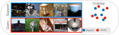
(a) Standard FSL

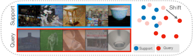
(b) FSL under Support / Query Shift

Figure 1: Illustration of the FSQS problem with a 5-way 1-shot classification task sampled from the miniImageNet dataset [76]. In (a), a standard FSL setting where support and query sets are sampled from the same distribution. In (b), the same task but with shot-noise and contrast perturbations from [16] applied on support and query sets (respectively) that results in a support-query shift. In the latter case, a similarity measure based on the Euclidean metric [73] may become inadequate.

The situation of Distribution Shift (DS) i.e., when training and testing distributions differ, is ubiquitous and has dramatic effects on deep models [16], motivating works in Unsupervised Domain Adaptation [67], Domain Generalization [14] or Test-Time Adaptation [77]. However, the state of the art brings insufficient knowledge on few-shot learners’ behaviours when facing distribution shift. Some pioneering works demonstrate that advanced FSL algorithms do not handle cross-domain generalization better than more naive approaches [42]. Despite its great practical interest, FSL under distribution shift between the support and query sets is an under-investigated problem and attracts a very recent attention [11]. We refer to it as Few-Shot Learning under Support/Query Shift (FSQS) and provide an illustration in Figure 1. It reflects a more realistic situation where the algorithm is fed with a support set at the time of deployment and infers continuously on data subject to shift. The first solution is to re-acquire a support set that follows the data’s evolution. Nevertheless, it implies human intervention to select and annotate data to update an already deployed model, reacting to a potential drop in performances. The second solution consists in designing an algorithm that is robust to the distribution shift encountered during inference. This is the subject of the present work. Our contributions are:

1. FewShiftBed: a testbed for FSQS available at https://github.com/ebennequin/meta-domain-shift. The testbed includes 3 challenging benchmarks along with a protocol for fair and rigorous comparison across methods as well as an implementation of relevant baselines, and an interface to facilitate the implementation of new methods.

2. We conduct extensive experimentation of a representative set of few-shot algorithms. We empirically show that Transductive Batch-Normalization [3] mitigates an important part of the inopportune effect of FSQS.

3. We bridge Unsupervised Domain Adaptation (UDA) with FSL to address FSQS. We introduce Transported Prototypes, an efficient transductive algorithm that couples Optimal Transport (OT) [23] with the celebrated Prototypical Networks [73]. The use of OT follows a long-standing history in UDA for aligning representations between distributions [37, 50]. Our experiments demonstrate that OT shows a remarkable ability to perform this alignment even with only a few samples to compare distributions and provide a simple but strong baseline.

In Section 2 we provide a formal statement of FSQS, and we position this new problem among existing learning paradigms. In Section 3, we present FewShiftBed. We detail the datasets, the chosen baselines, and a protocol that guarantees a rigorous and reproducible evaluation. In Section 3, we present a method that couples Optimal Transport with Prototypical Networks [73]. Finally, in Section 5, we conduct an extensive evaluation of baselines and our proposed method using the testbed.

2 The Support-Query Shift problem

2.1 Statement

Notations.

We consider an input space $\mathcal{X}$, a representation space $\mathcal{Z}\subset\mathbb{R}^{d}$ ($d>0$) and a set of classes $\mathsf{C}$. A representation is a learnable function from $\mathcal{X}$ to $\mathcal{Z}$ and is noted $\varphi(\cdot;\theta)$ with $\theta\in\Theta$ for $\Theta$ a set of parameters. A dataset is a set $\Delta(\mathsf{C},\mathsf{D})$ defined by a set of classes $\mathsf{C}$ and a set of domains $\mathsf{D}$ i.e., a domain $\mathcal{D}\in\mathsf{D}$ is a set of IID realizations from a distribution noted $p_{\mathcal{D}}$. For two domains $\mathcal{D},\mathcal{D}^{\prime}\in\mathsf{D}$, the distribution shift is characterized by $p_{\mathcal{D}}\neq p_{\mathcal{D}^{\prime}}$. For instance, if the data consists of images of letters handwritten by several users, $\mathcal{D}$ can consist of samples from a specific user. Referring to the well known UDA terminology of source / target [67], we define a couple of source-target domains as a couple $(\mathcal{D}_{s},\mathcal{D}_{t})$ with $p_{\mathcal{D}_{s}}\neq p_{\mathcal{D}_{t}}$, thus presenting a distribution shift. Additionally, given $\mathcal{C}\subset\mathsf{C}$ and $\mathcal{D}\in\mathsf{D}$, the restriction of a domain $\mathcal{D}$ to images with a label that belongs to $\mathcal{C}$ is noted $\mathcal{D}^{\mathcal{C}}$.

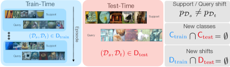
Figure 2: During meta-learning (Train-Time), each episode contains a support and a query set sampled from different distributions (for instance, illustrated by noise and contrasts as in Figure 1(b)) from a set of training domains ($\mathsf{D}_{\mathrm{train}}$), reflecting a situation that may potentially occurs at test-time. When deployed, the FSL algorithm using a trained backbone is fed with a support set sampled from new classes. As the algorithm is subject to infer continuously on data subject to shift (Test-Time), we evaluate the algorithm on data with an unknown shift ($\mathsf{D}_{\mathrm{test}}$). Importantly, both classes (${\mathsf{C}}_{\mathrm{train}}\cap{\mathsf{C}}_{\mathrm{test}}=\emptyset$) and shifts ($\mathsf{D}_{\mathrm{train}}\cap\mathsf{D}_{\mathrm{test}}=\emptyset$) are not seen during training, making the FSQS a challenging problem of generalization.

Dataset splits.

We build a split of $\Delta(\mathsf{C},\mathsf{D})$, by splitting $\mathsf{D}$ (respectively $\mathsf{C}$) into $\mathsf{D}_{\text{train}}$ and $\mathsf{D}_{\text{test}}$ (respectively $\mathsf{C}_{\text{train}}$ and $\mathsf{C}_{\text{test}}$) such that $\mathsf{D}_{\text{train}}\cap\mathsf{D}_{\text{test}}=\emptyset$ and $\mathsf{D}_{\text{train}}\cup\mathsf{D}_{\text{test}}=\mathsf{D}$ (respectively $\mathsf{C}_{\text{train}}\cap\mathsf{C}_{\text{test}}=\emptyset$ and $\mathsf{C}_{\text{train}}\cup\mathsf{C}_{\text{test}}=\mathsf{C}$). This gives us a train/test split with the datasets $\Delta_{\text{train}}=\Delta(\mathsf{C}_{\text{train}},\mathsf{D}_{\text{train}})$ and $\Delta_{\text{test}}=\Delta(\mathsf{C}_{\text{test}},\mathsf{D}_{\text{test}})$. By extension, we build a validation set following the same protocol.

Few-Shot Learning under Support-Query Shift (FSQS).

Given:

• $\mathsf{D}^{\prime}\in\{\mathsf{D}_{\mathrm{train}},\mathsf{D}_{\mathrm{test}}\}$ and $\mathsf{C}^{\prime}\in\{\mathsf{C}_{\mathrm{train}},\mathsf{C}_{\mathrm{test}}\}$,

• a couple of source-target domains $(\mathcal{D}_{s},\mathcal{D}_{t})$ from $\mathsf{D}^{\prime}$,

• a set of classes $\mathcal{C}\subset\mathsf{C}^{\prime}$;

• a small labelled support set $\mathcal{S}={(x_{i},y_{i})}_{i=1,\dots,|\mathcal{S}|}$ (named source support set) such that for all $i$, $y_{i}\in\mathcal{C}$ and $x_{i}\in\mathcal{D}_{s}$ i.e., $\mathcal{S}\subset\mathcal{D}_{s}^{\mathcal{C}}$;

• an unlabelled query set $\mathcal{Q}={(x_{i})}_{i=1,\dots,|\mathcal{Q}|}$ (named target query set) such that for all $i$, $y_{i}\in\mathcal{C}$ and $x_{i}\in\mathcal{D}_{t}$ i.e., $\mathcal{Q}\subset\mathcal{D}_{t}^{\mathcal{C}}$.

The task is to predict the labels of query set instances in $\mathcal{C}$. When $|\mathcal{C}|=n$ and the support set contains $k$ labelled instances for each class, this is called an $n$-way $k$-shot FSQS classification task. Note that this paradigm provides an additional challenge compared to classical Few-shot classification tasks, since at test time, the model is expected to generalize to both new classes and new domains while support set and query set are sampled from different distributions. This paradigm is illustrated in Figure 2.

Episodic training.

We build an episode by sampling some classes $\mathcal{C}\subset\mathsf{C}_{\text{train}}$, and a source and target domain $\mathcal{D}_{s},\mathcal{D}_{t}$ from $\mathsf{D}_{\text{train}}$. We build a support set $\mathcal{S}={(x_{i},y_{i})}_{i=1\dots|\mathcal{S}|}$ of instances from source domain $\mathcal{D}_{s}^{\mathcal{C}}$, and a query set $\mathcal{Q}={(x_{i},y_{i})}_{i=|\mathcal{S}|+1,\dots,|\mathcal{S}|+|\mathcal{Q}|}$ of instances from target domain $\mathcal{D}_{t}^{\mathcal{C}}$, such that $\forall i\in\left[1,|\mathcal{S}|+|\mathcal{Q}|\right]$, $y_{i}\in\mathcal{C}$. Using the labelled examples from $\mathcal{S}$ and unlabelled instances from $\mathcal{Q}$, the model is expected to predict the labels of $\mathcal{Q}$. The parameters of the model are then trained using a cross-entropy loss between the predicted labels and ground truth labels of the query set.

2.2 Positioning and Related Works

To highlight FSQS’s novelty, our discussion revolves around the problem of inferring on a given Query Set provided with the knowledge of a Support Set. We refer to this class of problems as SQ problems. Intrinsically, FSL falls into the category of SQ problems. Interestingly, Unsupervised Domain Adaptation [67] (UDA), defined as labelling a dataset sampled from a target domain based on labelled data sampled from a source domain, is also a SQ problem. Indeed, in this case, the source domain plays the role of support, while the target domain plays the query’s role. Notably, an essential line of study in UDA leverages the target data distribution for aligning source and target domains, reflecting the importance of transduction in a context of adaptation [37, 50] i.e., performing prediction by considering all target samples together. Transductive algorithms also have a special place in FSL [48, 60, 70] and show that leveraging a query set as a whole brings a significant boost in performances. Nevertheless, UDA and FSL exhibit fundamental differences. UDA addresses the problem of distribution shift using important source data and target data (typically thousands of instances) to align distributions. In contrast, FSL focuses on the difficulty of learning from few samples. To this purpose, we frame UDA as both SQ problem with large transductivity and Support / Query Shift, while Few-Shot Learning is a SQ problem, eventually with small transductivity for transductive FSL. Thus, FSQS combines both challenges: distribution shift and small transductivity. This new perspective allows us to establish fruitful connections with related learning paradigms, presented in Table 1, that we review in the following. A thorough review is available in Appendix A.

SQ problems Train-Time Test-Time Support Query Support Query New New Size Labels Size Labels Size Labels Transductivity classes domains   No SQS FSL [73, 49] Few ✓ Few ✓ Few ✓ Point-wise ✓ ✗ TransFSL [70, 60] Few ✓ Few ✓ Few ✓ Small ✓ ✗ CDFSL [42] Few ✓ Few ✓ Few ✓ Point-wise ✓ ✓   SQS UDA [68, 67] Large ✓ Large TTA [74, 72, 77] Large ✓ Small ✓ ARM [82] Large ✓ Few ✓ Small ✓ Ind FSQS Few ✓ Few ✓ Few ✓ Point-wise ✓ ✓ Trans FSQS Few ✓ Few ✓ Few ✓ Small ✓ ✓

Table 1: An overview of SQ problems. We divide SQ problems into two categories, presence or not of Support-Query shift; No SQS vs SQS. We consider three classes of transductivity: point-wise transductivity that is equivalent to inductive inference, small transductivity when inference is performed at batch level (typically in [77, 82]), and large transductivity when inference is performed at dataset level (typically in UDA). New classes (resp. new domains) describe if the model is evaluated at test-time on novel classes (resp. novel domains). Note that we frame UDA as a fully test-time algorithm. Notably, Cross-Domain FSL (CDFSL) [42] assumes that the support set and query set are drawn from the same distribution, thus No SQS.

Adaptation.

Unsupervised Domain Adaptation (UDA) requires a whole target dataset for inference, limiting its applications. Recent pioneering works, referred to as Test-Time Adaptation (TTA), adapt at test-time a model provided with a batch of samples from the target distribution. The proposed methodologies are test-time training by self-supervision [74], updating batch-normalization statistics [72] or parameters [77], or meta-learning to condition predictions on the whole batch of test samples for an Adaptative Risk Minimization (ARM) [82]. Inspired from the principle of invariant representations [37, 50], the seminal work [46] brings Optimal Transport (OT) [23] as an efficient framework for aligning data distributions. OT has been recently applied in a context of transductive FSL [54] and our proposal (TP) is to provide a simple and strong baseline following the principle of OT as it is applied in UDA. In this work, following [3], we also study the role of Batch-Normalization for SQS, that points out the role of transductivity. Our conviction was that the batch-normalization is the first lever for aligning distributions [72, 77].

Few-Shot Classification.

We usually frame Few-Shot Classification methods [42] as either metric-based methods [76, 73], or optimization-based methods that learn to fine-tune by adapting with few gradient steps [49]. A promising line of study leverages transductivity (using the query set as unlabelled data while inductive methods predict individually on each query sample). Transductive Propagation Network [60] meta-learns label propagation from the support to query set concurrently with the feature extractor. Transductive Fine-Tuning [48] minimizes the prediction entropy of all query instances during fine-tuning. Evaluating cross-domain generalization of FSL (FSCD), i.e., a distributional shift between meta-training and meta-testing, attracts the attention of a few recent works [42]. Zhao et al. propose a Domain-Adversarial Prototypical Network [84] in order to both align source and target domains in the feature space while maintaining discriminativeness between classes. Sahoo et al. combine Prototypical Networks with adversarial domain adaptation at the task level [71]. Notably, Cross-Domain Few-Shot Learning [42] (CDFSL) addresses the distributional shift between meta-training and meta-testing assuming that the support set and query set are drawn from the same distribution, not making it a SQ problem with support-query shift. Concerning the novelty of FSQS, we acknowledge the very recent contribution of Du et al. [11] which studies the role of learnable normalization for domain generalization, in particular when support and query sets are sampled from different domains. Note that our statement is more ambitious: we evaluate algorithms on both source and target domains that were unseen during training, while in their setting the source domain has already been seen during training.

Benchmarks in Machine Learning

Releasing benchmark has always been an important factor for progress in the Machine Learning field, the most outstanding example being ImageNet [9] for the Computer Vision community. Recently, DomainBed [14] aims to settle Domain Generalization research into a more rigorous process, where FewShiftBed takes inspiration from it. Meta-Dataset [30] is an other example, this time specific to FSL.

3 FewShiftBed: A Pytorch testbed for FSQS

3.1 Datasets

We designed three new image classification datasets adapted to the FSQS problem. These datasets have two specificities.

1. They are dividable into groups of images, assuming that each group corresponds to a distinct domain. A key challenge is that each group must contain enough images with a sufficient variety of class labels, so that it is possible to sample FSQS episodes.

2. They are delivered with a train/val/test split ($\Delta_{\text{train}},\Delta_{\text{val}},\Delta_{\text{test}}$), along both the class and the domain axis. This split is performed following the principles detailed in Section 2. Therefore, these datasets provide true few-shot tasks at test time, in the sense that the model will not have seen any instances of test classes and domains during training. Note that since we split along two axes, some data may be discarded (for instance images from a domain in $\mathsf{D}_{\text{train}}$ with a label in $\mathsf{C}_{\text{test}}$). Therefore it is crucial to find a split that minimizes this loss of data.

Meta-CIFAR100-Corrupted (MC100-C).

CIFAR-100 [19] is a dataset of 60k three-channel square images of size $32\times 32$, evenly distributed in 100 classes. Classes are evenly distributed in 20 superclasses. We use the same method used to build CIFAR-10-C [16], which makes use of 19 image perturbations, each one being applied with 5 different levels of intensity, to evaluate the robustness of a model to domain shift. We modify their protocol to adapt it to the FSQS problem: (i) we split the classes with respect to the superclass structure, and assign 13 superclasses (65 classes) to the training set, 2 superclasses (10 classes) to the validation set, and 5 superclasses (25 classes) to the testing set; (ii) we also split image perturbations (acting as domains), following the split of [82]. We obtain 2,184k transformed images for training, 114k for validation and 330k for testing. The detailed split is available in the documentation of our code repository.

miniImageNet-Corrupted (mIN-C).

miniImageNet [76] is a popular benchmark for few-shot image classification. It contains 60k images from 100 classes from the ImageNet dataset. 64 classes are assigned to the training set, 16 to the validation set and 20 to the test set. Like MC100-C, we build mIN-C using the image perturbations proposed by [16] to simulate different domains. We use the original split from [76] for classes, and use the same domain split as for MC100-C. Although the original miniImageNet uses $84\times 84$ images, we use $224\times 224$ images. This allows us to re-use the perturbation parameters calibrated in [16] for ImageNet. Finally, we discard the 5 most time-consuming perturbations. We obtain a total of 1.2M transformed images for training, 182k for validation and 228k for testing. The detailed split in the documentation of our code repository.

FEMNIST-FewShot (FEMNIST-FS).

EMNIST [6] is a dataset of images of handwritten digits and uppercase and lowercase characters. Federated-EMNIST [4] is a version of EMNIST where images are sorted by writer (or user). FEMNIST-FS consists in a split of the FEMNIST dataset adapted to few-shot classification. We separate both users and classes between training, validation and test sets. We build each group as the set of images written by one user. The detailed split is available in the code. Note that in FEMNIST, many users provide several instances for each digits, but less than two instance for most letters. Therefore it is hard to find enough samples from a user to build a support set or a query set. As a result, our experiments are limited to classification tasks with only one sample per class in both the support and query sets.

3.2 Algorithms

We implement in FewShiftBed two representative methods of the vast literature of FSL, that are commonly considered as strong baselines: Prototypical Networks (ProtoNet) [73] and Matching Networks (MatchingNet) [76]. Besides, for transductive FSL, we also implement with Transductive Propagation Network (TransPropNet) [60] and Transductive Fine-Tuning (FTNet) [48]. We also implement our novel algorithm Transported Prototypes (TP) which is detailed in Section 3. FewShiftBed is designed for favoring a straightforward implementation of a new algorithm for FSQS. To add a new algorithm, we only need to implement the set_forward method of the class AbstractMetaLearner. We provide an example with our implementation of the Prototypical Network [73] that only requires few line of codes:

⬇

class ProtoNet(AbstractMetaLearner):

def set_forward(self, support_images, support_labels, query_images):

z_support, z_query = self.extract_features(support_images, query_images)

z_proto = self.get_prototypes(z_support, support_labels)

return - euclidean_dist(z_query, z_proto)

3.3 Protocol

To prevent the pitfall of misinterpreting a performance boost, we draw three recommendations to isolate the causes of improvement rigorously.

• How important is episodic training? Despite its wide adoption in meta-learning for FSL, in some situation episodic training does not perform better than more naive approaches [42]. Therefore we recommend to report both the result obtained using episodic training and standard ERM (see the documentation of our code repository).

• How does the algorithm behave in the absence of Support-Query Shift? In order to assess that an algorithm designed for distribution shift does not provide degraded performance in an ordinary concept, and to provide a top-performing baseline, we recommend reporting the model’s performance when we do not observe, at test-time, a support-query shift. Note that it is equivalent to evaluate the performance in cross-domain generalization, as firstly described in [42].

• Is the algorithm transductive? The assumption of transductivity has been responsible of several improvements in FSL [70, 3] while it has been demonstrated in [3] that MAML [49] benefits strongly from the Transductive Batch-Normalization (TBN). Thus, we recommend specifying if the method is transductive and adapting the choice of the batch-normalization accordingly (Conventional Batch Normalization [18] and Transductive Batch Normalization for inductive and transductive methods, respectively) since transductive batch normalization brings a significant boost in performance [3].

4 Transported Prototypes: A baseline for FSQS

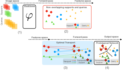
Figure 3: Overview of Transported Prototypes. (1) A support set and a query set are fed to a trained backbone that embeds images into a feature space. (2) Due to the shift between distributions, support and query instances are embedded in non-overlapping areas. (3) We compute the Optimal Transport from support instances to query instances to build the transported support set. Note that we represent the transport plan only for one instance per class to preserve clarity in the schema. (4) Provided with the transported support, we apply the Prototypical Network [73] i.e., $L^{2}$ similarity between transported support and query instances.

4.1 Overall idea

We present a novel method that brings UDA to FSQS. As aforementioned, FSQS presents new challenges since we no longer assume that we sample the support set and the query set from the same distribution. As a result, it is unlikely that the support set and query sets share the same representation space region (non-overlap). In particular, the $L^{2}$ distance, adopted in the celebrated Prototypical Network [73], may not be relevant for measuring similarity between query and support instances, as presented in Figure 1. To overcome this issue, we develop a two-phase approach that combines Optimal Transport (Transportation Phase) and the celebrated Prototypical Network (Prototype Phase). We give some background about Optimal Transport (OT) in Section 4.2 and the whole procedure is presented in Algorithm 1.

4.2 Background

Definition.

We provide some basics about Optimal Transport (OT). A thorough presentation of OT is available at [23]. Let $p_{s}$ and $p_{t}$ be two distributions on $\mathcal{X}$, we note $\Pi(p_{s},p_{t})$ the set of joint probability with marginal $p_{s}$ and $p_{t}$ i.e., $\forall\pi\in\Pi(p_{s},p_{t}),\forall x\in\mathcal{X},\pi(\cdot,x)=p_{s},\pi(x,\cdot)=p_{t}$. The Optimal Transport, associated to cost $c$, between $p_{s}$ and $p_{t}$ is defined as:

$$W_{c}(p_{s},p_{t}):=\min_{\pi\in\Pi(p_{s},p_{t})}\mathbb{E}_{(x_{s},x_{t})\sim\pi}\left[c(x_{s},x_{t})\right]$$ (1)

with $c(\cdot,\cdot)$ any metric. We note $\pi^{\star}(p_{s},p_{t})$ the joint distribution that achieves the minimum in equation 1. It is named the transportation plan from $p_{s}$ to $p_{t}$. When there is no confusion, we simply note $\pi^{\star}$. For our applications, we will use as metric the euclidean distance in the representation space obtained from a representation $\varphi(\cdot;\theta)$ i.e., $c_{\theta}(x_{s},x_{t}):=||\varphi(x_{s};\theta)-\varphi(x_{t};\theta)||_{2}$.

Discrete OT.

When $p_{s}$ and $p_{t}$ are only accessible through a finite set of samples, respectively $(x_{s,1},...,x_{s,n_{s}})$ and $(x_{t,1},...,x_{t,n_{t}})$ we introduce the empirical distributions $\hat{p}_{s}:=\sum_{i=1}^{n_{s}}w_{s,i}\delta_{x_{s,i}},~{}~{}\hat{p}_{t}:=\sum_{j=1}^{n_{t}}w_{t,j}\delta_{x_{t,j}}$, where $w_{s,i}$ ($w_{t,j}$) is the mass probability put in sample $x_{s,i}$ ($x_{t,j}$) i.e., $\sum_{i=1}^{n_{s}}w_{s,i}=1$ ($\sum_{j=1}^{n_{t}}w_{t,j}=1$) and $\delta_{x}$ is the Dirac distribution in $x$. The discrete version of the OT is derived by introducing the set of couplings $\mathbf{\Pi}(p_{s},p_{t}):=\left\{\bm{\pi}\in\mathbb{R}^{n_{s}\times n_{t}},\bm{\pi}\mathbf{1}_{n_{s}}=\mathbf{p}_{s},\bm{\pi}^{\top}\mathbf{1}_{n_{t}}=\mathbf{p}_{t}\right\}$ where $\mathbf{p}_{s}:=(w_{s,1},\cdots,w_{s,n_{s}})$, $\mathbf{p}_{t}:=(w_{t,1},\cdots,w_{1,n_{t}})$, and $\mathbf{1}_{n_{s}}$ (respectively $\mathbf{1}_{n_{t}}$) is the unit vector with dim $n_{s}$ (respectively $n_{t}$). The discrete transportation plan $\bm{\pi}^{\star}_{\theta}$ is then defined as:

$$\bm{\pi}_{\theta}^{\star}:=\underset{\bm{\pi}\in\mathbf{\Pi}(p_{s},p_{t})}{\mathrm{argmin}}\langle\bm{\pi},\mathbf{C}_{\theta}\rangle_{F}$$ (2)

where $\mathbf{C}_{\theta}(i,j):=c_{\theta}(x_{s,i},x_{t,j})$ and $\langle\cdot,\cdot\rangle_{F}$ is the Frobenius dot product. Note that $\bm{\pi}^{\star}_{\theta}$ depends on both $p_{s}$ and $p_{t}$, and $\theta$ since $\mathbf{C}_{\theta}$ depends on $\theta$. In practice, we use Entropic regularization [47] that makes OT easier to solve by promoting smoother transportation plan with a computationally efficient algorithm, based on Sinkhorn-Knopp’s scaling matrix approach (see the Appendix C).

4.3 Method

Algorithm 1 Transported Prototypes. Blue lines highlight the OT’s contribution in the computational graph of an episode compared to the standard Prototypical Network [73].

Input: Support set $\mathcal{S}:=(x_{s,i},y_{s,i})_{1\leq i\leq n_{s}}$, query set $\mathcal{Q}:=(x_{q,j},y_{q,j})_{1\leq j\leq n_{q}}$, classes $\mathcal{C}$, backbone $\varphi_{\theta}$.
Output: Loss $\mathcal{L}(\theta)$ for a randomly sampled episode.

1:$z_{s,i},z_{q,j}\leftarrow\varphi(x_{s,i};\theta),\varphi(x_{q,j};\theta)$, for $i,j$ $\triangleright$ Get representations.

2:$\mathbf{C}_{\theta}(i,j)\leftarrow||z_{s,i}-z_{q,j}||^{2}$, for $i,j$ $\triangleright$ Cost-matrix.

3:$\bm{\pi}_{\theta}^{\star}\leftarrow$ Solve Equation 2 $\triangleright$ Transportation plan.

4:$\hat{\bm{\pi}}_{\theta}^{\star}(i,j)\leftarrow\bm{\pi}^{\star}_{\theta}(i,j)/\sum_{j}\bm{\pi}_{\theta}^{\star}(i,j)$, for $i,j$ $\triangleright$ Normalization.

5:$\hat{\mathbf{S}}=(\hat{z}_{s,i})_{i}\leftarrow$ Given by Equation 3 $\triangleright$ Get transported support set.

6:$\hat{\mathbf{c}}_{k}\leftarrow\frac{1}{|\hat{\mathbf{S}}_{k}|}\sum_{\hat{z}_{s}\in\hat{\mathbf{S}}_{k}}\hat{z}_{s}$, for $k\in\mathcal{C}$. $\triangleright$ Get transported prototypes.

7:$p_{\theta}(y|x_{q,j})\leftarrow$ From Equation 4, for $j$

8:Return: $\mathcal{L}(\theta):=\frac{1}{n_{q}}\sum_{j=1}^{n_{q}}-\log p_{\theta}(y_{q,j}|x_{q,j})$.

Transportation Phase.

At each episode, we are provided with a source support set $\mathcal{S}$ and a target query set $\mathcal{Q}$. We note respectively $\mathbf{S}$ and $\mathbf{Q}$ their representations from a deep network $\varphi(\cdot;\theta)$ i.e., $z_{s}\in\mathbf{S}$ is defined as $z_{s}:=\varphi(x_{s};\theta)$ for $x_{s}\in\mathcal{S}$, respectively $z_{q}\in\mathbf{Q}$ is defined as $z_{q}:=\varphi(x_{q};\theta)$ for $x_{q}\in\mathcal{Q}$. As these two sets are sampled from different distributions, $\mathbf{S}$ and $\mathbf{Q}$ are likely to lie in different regions of the representation space. In order to adapt the source support set $\mathcal{S}$ to the target domain, which is only represented by the target query set $\mathcal{Q}$, we follow [46] to compute $\hat{\mathbf{S}}$ the barycenter mapping of $\mathcal{S}$, that we refer to as the transported support set, defined as follows:

$$\hat{\mathbf{S}}:=\hat{\bm{\pi}}_{\theta}^{\star}\mathbf{Q}$$ (3)

where $\bm{\pi}_{\theta}^{\star}$ is the transportation plan from $\mathbf{S}$ to $\mathbf{Q}$ and $\hat{\bm{\pi}}^{\star}_{\theta}:=\bm{\pi}^{\star}_{\theta}(i,j)/\sum_{j=1}^{n_{t}}\bm{\pi}^{\star}_{\theta}(i,j)$. The transported support set $\hat{\mathbf{S}}$ is an estimation of labelled examples in the target domain using labelled examples in the source domain. The success relies on the fact that transportation conserves labels, i.e., a query instance close to $\hat{z_{s}}\in\hat{\mathbf{S}}$ should share the same label with $x_{s}$, where $\hat{z_{s}}$ is the barycenter mapping of $z_{s}\in\mathbf{S}$. See step (3) of Figure 3 for a visualization of the transportation phase.

Prototype Phase.

For each class $k\in\mathcal{C}$, we compute the transported prototypes $\hat{\mathbf{c}}_{k}:=\frac{1}{|\hat{\mathbf{S}}_{k}|}\sum_{\hat{z}_{s}\in\hat{\mathbf{S}}_{k}}\hat{z}_{s}$ (where $\hat{\mathbf{S}}_{k}$ is the transported support set with class $k$ and $\mathcal{C}$ are classes of current episode). We classify each query $x_{q}$ with representation $z_{q}=\varphi(x_{q};\theta)$ using its euclidean distance to each transported prototypes;

$$p_{\theta}(y=k|x_{q}):=\frac{\exp\left(-||z_{q}-\hat{\mathbf{c}}_{k}||^{2}\right)}{\sum_{k^{\prime}\in\mathcal{C}}\exp\left(-||z_{q}-\hat{\mathbf{c}}_{k^{\prime}}||^{2}\right)}$$ (4)

Crucially, the standard Prototypical Networks [73] computes euclidean distance to each prototypes while we compute the euclidean to each transported prototypes, as presented in step (4) of Figure 3. Note that our formulation involves the query set in the computation of $(\hat{\mathbf{c}}_{k})_{k\in\mathcal{C}}$.

Genericity of OT.

FewShiftBed implements OT as a stand-alone module that can be easily plugged into any FSL algorithm. We report additional baselines in Appendix B where other FSL algorithms are equipped with OT. This technical choice reflects our insight that OT may be ubiquitous for addressing FSQS and makes its usage in the testbed straightforward.

5 Experiments

	Meta-CIFAR100-C		miniImageNet-C		FEMNIST-FS
	1-shot	5-shot	1-shot	5-shot	1-shot
ProtoNet [73]	30.02 $\pm$ 0.40	42.77 $\pm$ 0.47	36.37 $\pm$ 0.50	47.58 $\pm$ 0.57	84.31 $\pm$ 0.73
MatchingNet [76]	30.71 $\pm$ 0.38	41.15 $\pm$ 0.45	35.26 $\pm$ 0.50	44.75 $\pm$ 0.55	84.25 $\pm$ 0.71
TransPropNet${\dagger}$ [60]	34.15 $\pm$ 0.39	47.39 $\pm$ 0.42	24.10 $\pm$ 0.27	27.24 $\pm$ 0.33	86.42 $\pm$ 0.76
FTNet${\dagger}$ [48]	28.91 $\pm$ 0.37	37.28 $\pm$ 0.40	39.02 $\pm$ 0.46	51.27 $\pm$ 0.45	86.13 $\pm$ 0.71
TP${\dagger}$ (ours)	34.00 $\pm$ 0.46	49.71 $\pm$ 0.47	40.49 $\pm$ 0.54	59.85 $\pm$ 0.49	93.63 $\pm$ 0.63
TP w/o OT ${\dagger}$	32.47 $\pm$ 0.41	48.00 $\pm$ 0.44	40.43 $\pm$ 0.49	53.71 $\pm$ 0.50	90.36 $\pm$ 0.58
TP w/o TBN ${\dagger}$	33.74 $\pm$ 0.46	49.18 $\pm$ 0.49	37.32 $\pm$ 0.55	55.16 $\pm$ 0.54	92.31 $\pm$ 0.73
TP w. OT-TT ${\dagger}$	32.81 $\pm$ 0.46	48.62 $\pm$ 0.48	44.77 $\pm$ 0.57	60.46 $\pm$ 0.49	94.92 $\pm$ 0.55
TP w/o ET ${\dagger}$	35.94 $\pm$ 0.45	48.66 $\pm$ 0.46	42.46 $\pm$ 0.53	54.67 $\pm$ 0.48	94.22$\pm$ 0.70
TP w/o SQS ${\dagger}$	85.67 $\pm$ 0.26	88.52 $\pm$ 0.17	64.27 $\pm$ 0.39	75.22 $\pm$ 0.30	99.72 $\pm$ 0.07

Table 2: Top-1 accuracy of few-shot learning models in various datasets and numbers of shots with 8 instances per class in the query set (except for FEMNIST-FS: 1 instance per class in the query set), with 95% confidence intervals. The top half of the table is a comparison between existing few-shot learning methods and Transported Prototypes (TP). The bottom half is an ablation study of TP. OT denotes Optimal Transport, TBN is Transductive Batch-Normalization, OT-TT refers to the setting where Optimal Transport is applied at test time but not during episodic training, and ET means episodic training i.e., w/o ET refers to the setting where training is performed through standard Empirical Risk Minimization. TP w/o SQS reports model’s performance in the absence of support-query shift. ${\dagger}$ flags if the method is transductive. For each setting, the best accuracy among existing methods is shown in bold, as well as the accuracy of an ablation if it improves TP.

We compare the performance of baseline algorithms with Transported Prototypes on various datasets and settings. We also offer an ablation study in order to isolate the source to the success of Transported Prototypes. Extensive results are detailed in Appendix B. Instructions to reproduce these results can be found in the code’s documentation.

Setting and details.

We conduct experiments on all methods and datasets implemented in FewShiftBed. We use a standard 4-layer convolutional network for our experiments on Meta-CIFAR100-C and FEMNIST-FewShot, and a ResNet18 for our experiments on miniImageNet. Transductive methods are equipped with a Transductive Batch-Normalization. All episodic training runs contain 40k episodes, after which we retrieve model state with best validation accuracy. We run each individual experiment on three different random seeds. All results presented in this paper are the average accuracies obtained with these random seeds.

Analysis.

The top half of Table 2 reveals that Transported Prototypes (TP) outperform all baselines by a strong margin on all datasets and settings. Importantly, baselines perform poorly on FSQS, demonstrating they are not equipped to address this challenging problem, stressing our study’s significance. It is also interesting to note that the performance of transductive approaches, which is significantly better in a standard FSL setting [60, 48], is here similar to inductive methods (notably, TransPropNet [60] fails loudly without Transductive Batch-Normalization showing that propagating label with non-overlapping support/query can have a dramatic impact, see Appendix B). Thus, FSQS deserves a fresher look to be solved. Transported Prototypes mitigate a significant part of the performance drop caused by support-query shift while benefiting from the simplicity of combining a popular FSL method with a time-tested UDA method. This gives us strong hopes for future works in this direction.

Ablation study.

Transported Prototypes (TP) combines three components: Optimal Transport (OT), Transductive Batch-Normalization (TBN) and episode training (ET). Which of these components are responsible for the observed gain? Following recommendations from Section 3.3, we ablate those components in the bottom half of Table 2. We observe that both OT and TBN individually improve the performance of ProtoNet for FSQS, and that the best results are obtained when the two of them are combined. Importantly, OT without TBN performs better than TBN without OT (except for 1-shot mIN-C), demonstrating the superiority of OT compared to TBN for aligning distributions in the few samples regime. Note that the use of TaskNorm [3] is beyond the scope of the paper; we encourage future work to dig into that direction and we refer the reader to the very recent work [11]. We observe that there is no clear evidence that using OT at train-time is better than simply applying it at test-time on a ProtoNet trained without OT. Additionally, the value of Episodic Training (ET) compared to standard Empirical Risk Minimization (ERM) is not obvious. For instance, simply training with ERM and applying TP at test-time is better than adding ET on 1-shot MC100-C, 1-shot mIN-C and FEMNIST-FS, making it an another element to add to the study [20] who put into question the value of ET. Understanding why and when we should use ET or only OT at test-time is interesting for future works. Additionally, we compare TP with MAP [54] which implements an OT-based approach for transductive FSL. Their approach includes a power transform to reduce the skew in the distribution, so for fair comparison we also implemented it into Transported Prototypes for these experiments. We also used the OT module only at test-time and compared with two backbones, respectively trained with ET and ERM. Interestingly, our experiments in Table 3 show that MAP is able to handle SQS. Finally, in order to evaluate the performance drop related to Support-Query Shift compared to a setting with support and query instances sampled from the same distribution, we test Transported Prototypes on few-shot classification tasks without SQS (TP w/o SQS in Table 2), making a setup equivalent to CDFSL. Note that in both cases, the model is trained in an episodic fashion on tasks presenting a Support-Query Shift. These results show that SQS presents a significantly harder challenge than CDFSL, while there is considerable room for improvements.

	Meta-CIFAR100-C		miniImageNet-C		FEMNIST-FS
	1-shot	5-shot	1-shot	5-shot	1-shot
TP⋆	36.17 $\pm$ 0.47	50.45 $\pm$ 0.47	45.41 $\pm$ 0.54	57.82 $\pm$ 0.48	93.60 $\pm$ 0.68
MAP⋆	35.96 $\pm$ 0.44	49.55 $\pm$ 0.45	43.51 $\pm$ 0.47	56.10 $\pm$ 0.43	92.86 $\pm$ 0.67
TP†	32.13 $\pm$ 0.45	46.19 $\pm$ 0.47	45.77 $\pm$ 0.58	59.91 $\pm$ 0.48	94.92 $\pm$ 0.56
MAP†	32.38 $\pm$ 0.41	45.96 $\pm$ 0.43	43.81 $\pm$ 0.47	57.70 $\pm$ 0.43	87.15 $\pm$ 0.66

Table 3: Top-1 accuracy with 8 instances per class in the query set when applying Transported Prototypes and MAP on two different backbones: $\star$ is standard ERM (i.e., without Episodic Training) and ${\dagger}$ is ProtoNet [73]. Transported Prototypes performs equally or better than MAP [54]. Here TP includes power transform in the feature space.

6 Conclusion

We release FewShiftBed, a testbed for the under-investigated and crucial problem of Few-Shot Learning when the support and query sets are sampled from related but different distributions, named FSQS. FewShiftBed includes three datasets, relevant baselines and a protocol for reproducible research. Inspired from recent progress of Optimal Transport (OT) to address Unsupervised Domain Adaptation, we propose a method that efficiently combines OT with the celebrated Prototypical Network [73]. Following the protocol of FewShiftBed, we bring compelling experiments demonstrating the advantage of our proposal compared to transductive counterparts. We also isolate factors responsible for improvements. Our findings suggest that Batch-Normalization is ubiquitous, as described in related works [3, 11], while episodic training, even if promising on paper, is questionable. As a lead for future works, FewShiftBed could be improved by using different datasets to model different domains, instead of using artificial transformations. Since we are talking about domain adaptation, we also encourage the study of accuracy as a function of the size of the target domain, i.e., the size of the query set. Moving beyond the transductive algorithm, as well as understanding when meta-learning brings a clear advantage to address FSQS remains an open and exciting problem. FewShiftBed brings the first step towards its progress.

Appendix 0.A Extended positioning

Few-Shot Classification.

Methods to solve the Few-Shot Classification problem [57] are usually put into one of these three categories [42]: metric-based, optimization-based, and hallucination-based. Most metric-learning methods are built on the principle of Siamese Networks [56], while also exploiting the meta-learning paradigm: they learn a feature extractor across training tasks [76]. Prototypical Networks [73] classify queries from their euclidean distances to one prototype embedding per class. Relation Networks [75] add an other deep network on top of Prototype Networks to replace the euclidean distance. Optimization-based methods use an other approach: learning to fine-tune. MAML [49] and Reptile [65] learn a good model initialization, i.e. model parameters that can adapt to a new task (with novel classes) in a small number of gradient steps. Other methods such as Meta-LSTM [69] and Meta-Networks [63] replace standard gradient descent by a meta-learned optimizer. Hallucination-based methods aim at augmenting the scarce labeled data, by hallucinating feature vectors [53], using Generative Adversarial Networks [35], or meta-learning [78]. Recent works also suggest that competitive results in Few-Shot Classification can be achieved with more simple methods based on fine-tuning [42, 51].

Transductive Few-Shot Classification.

Some methods aim at solving few-shot classification tasks by using the query set as unlabeled data. Transductive Propagation Network [60] meta-learns label propagation from the support to query set concurrently with the feature extractor. Antoniou & Storkey [36] proposed to use a meta-learned critic network to further adapt a classifier on the query set in an unsupervised setting. Ren et al. [70] extend Prototypical Networks in order to use the query set in the prototype computation. Transductive Information Maximization [39] aims at maximizing the mutual information between the features extracted from the query set and their predicted labels. Finally, Transductive Fine-Tuning [48] augments standard fine-tuning using the classification entropy of all query instances.

Unsupervised Domain Adaptation.

UDA has a long standing story [67, 68]. The analysis of the role of representations from [37] has led to wide literature based on domain invariant representations [50, 62]. Outstanding progress have been towards learning more domain transferable representations by looking for domain invariance. The tensorial product between representations and prediction promotes conditional domain invariance [61], the use of weights [41, 81, 40, 44] has dramatically improved the problem of label shift theoretically described in [83], hallucinating consistent target samples [59], penalizing high singular values of batch of representations [43] or by enforcing the favorable inductive bias of consistence through various data augmentation in the target domain [66]. Recent works address the problem of adaptation without source data [58, 80]. The seminal work [46], followed by [45, 38], brings Optimal Transport (OT) to UDA by transporting source samples in the target domain.

Test-Time Adaptation.

Test-time Adaptation (TTA) is the subject of recent pioneering works. In [74], adaptation is performed by test-time training of representations through a self-supervision task which consists in predicting the rotation of an image. This leads to a successful adaptation when the gradient of fine-tuning procedure is correlated with the gradient of the cross-entropy between the prediction and the label of the target sample, which is not available. Inspired from UDA methods based on domain invariance of representations, a line of works [64, 72] aims to align the mean and the variance of train and test distribution of representations. This is simply done by updating statistics of the batch-normalization layer. In a similar spirit of leveraging the batch-normalization layer for adaptation, [77] suggests to minimize prediction entropy on a batch of test samples, as suggested in semi-supervised learning [52]. As pointed by authors of [77], updating the whole network is inefficient and exposes to a risk of test batch overfit. To adress this problem, authors suggest to only update batch-normalization parameters for minimizing prediction’s entropy. The paradigm of Adaptative Risk Minimization (ARM) is introduced in [82]. ARM aims to adapt a classifier at test-time by conditioning its prediction on the whole batch of test samples (not only one sample). Authors demonstrate that such classifier is meta-trainable as long as the training data exposes a structure of group. Consequently, [82] is closer work to ours, while we have more ambitious perspectives as we address the problem of few-shot learning i.e., few-shot are available per class while new classes are discovered at test-time.

Few-Shot Classification under Distributional Shift.

Recent works on few-shot classification tackle the problem of distributional shift between the meta-training set and the meta-testing set. Chen et al. [42] compare the performance of state-of-the-art solutions to few-shot classification on a cross-domain setting (meta-training on miniImageNet [76] and meta-testing on Caltech-UCSD Birds 200 [79]). Zhao et al. propose a Domain-Adversarial Prototypical Network [84] in order to both align source and target domains in the feature space and maintain discriminativeness between classes. Considering the problem as a shift in the distribution of tasks (i.e. training and testing tasks are drawn from two distinct distributions), Sahoo et al. combine Prototypical Networks with adversarial domain adaptation at task level [71]. While these works address the key issue of distributional shift between meta-training and meta-testing, they assume that for each task, the support set and query set are always drawn from the same distribution. We find that this assumption rarely holds in practice. In this work we consider a distributional shift both between meta-training and meta-testing and between support and query set.

Appendix 0.B All experimental results

In this section we present the extended results of our experiments. Prototypical Networks, Matching Networks and Transductive Propagation Networks have been declined in 10 distinct versions:

• Original algorithms: episodic training, with Conventional Batch-Normalization (CBN) and not Optimal Transport (Vanilla);

• Episodic training and CBN, with Optimal Transport applied at test time (OT-TT);

• Episodic training and CBN, with Optimal Transport integrated into the algorithm both during training and testing (OT);

• Episodic training, with Transductive Batch-Normalization (TBN) and not Optimal Transport (Vanilla);

• Episodic training and TBN, with OT-TT;

• Episodic training and TBN, with OT;

• Standard Empirical Risk Minimization (ERM) instead of episodic training, with CBN and not Optimal Transport (Vanilla);

• ERM with CBN and OT;

• ERM with TBN and no Optimal Transport (Vanilla);

• ERM with TBN and OT.

Transductive Fine-Tuning (FTNet) is not compatible with episodic training. Also the integration of Optimal Transport into this algorithm is non trivial. Therefore we only applied FTNet with ERM and without OT.

Every result presented in the following tables is the average over three runs with three random seeds (1, 2 and 3). For clarity, we do not report the 95% confidence interval for each result. Keep in mind that this interval is different for each result, but we found that it is always greater than $\pm$ 0.2% and smaller than $\pm$ 0.8%.

Details of the experiments and instructions to reproduce them are available in the code.

	Meta-CIFAR100-C 1-shot 8-target
	Episodic training						Standard ERM
	CBN			TBN			CBN		TBN
	Vanilla	w. OT-TT	w. OT	Vanilla	w. OT-TT	w. OT	Vanilla	w. OT	Vanilla	w. OT
ProtoNet	30.02	32.11	33.74	32.47	32.81	34.00	29.10	35.48	29.79	35.4
MatchingNet	30.71	32.85	34.48	32.97	32.78	35.11	33.50	36.13	33.67	35.87
PropNet	30.26	28.70	26.87	34.15	29.48	27.68	23.33	31.08	22.55	31.20
FTNet							28.91		28.75

Table 4: Ablation for Meta-CIFAR100-C 1-shot 8-target.

	Meta-CIFAR100-C 1-shot 16-target
	Episodic training						Standard ERM
	CBN			TBN			CBN		TBN
	Vanilla	w. OT-TT	w. OT	Vanilla	w. OT-TT	w. OT	Vanilla	w. OT	Vanilla	w. OT
ProtoNet	29.98	32.24	35.63	32.52	31.72	36.20	29.02	35.89	29.61	35.94
MatchingNet	31.1	30.94	35.53	33.08	33.28	36.36	33.49	36.61	33.64	36.54
PropNet	30.82	32.39	31.15	34.83	33.53	31.33	26.81	33.9	27.92	34.10
FTNet							29.01		28.86

Table 5: Ablation for Meta-CIFAR100-C 1-shot 16-target.

	Meta-CIFAR100-C 5-shot 8-target
	Episodic training						Standard ERM
	CBN			TBN			CBN		TBN
	Vanilla	w. OT-TT	w. OT	Vanilla	w. OT-TT	w. OT	Vanilla	w. OT	Vanilla	w. OT
ProtoNet	42.77	47.54	48.37	48.00	48.62	49.71	44.89	48.61	46.59	48.66
MatchingNet	41.15	43.90	44.55	45.05	44.86	45.78	43.00	45.35	43.51	45.10
PropNet	39.13	40.60	25.68	47.39	40.47	27.29	29.32	39.82	29.50	29.82
FTNet							37.28		37.40

Table 6: Ablation of Meta-CIFAR100-C 5-shot 8-target.

	Meta-CIFAR100-C 5-shot 16-target
	Episodic training						Standard ERM
	CBN			TBN			CBN		TBN
	Vanilla	w. OT-TT	w. OT	Vanilla	w. OT-TT	w. OT	Vanilla	w. OT	Vanilla	w. OT
ProtoNet	42.07	48.26	48.25	46.49	48.71	49.94	44.67	48.61	46.48	48.89
MatchingNet	41.74	44.51	45.71	44.91	44.71	47.37	42.97	46.06	46.22	46.37
PropNet	38.73	39.25	37.22	43.91	40.62	40.02	33.06	40.03	33.93	40.03
FTNet							37.51		37.66

Table 7: Ablation of Meta-CIFAR100-C 5-shot 16-target.

	FEMNIST-FewShot 1-shot 1-target
	Episodic training						Standard ERM
	CBN			TBN			CBN		TBN
	Vanilla	w. OT-TT	w. OT	Vanilla	w. OT-TT	w. OT	Vanilla	w. OT	Vanilla	w. OT
ProtoNet	84.31	94.00	92.31	90.36	94.92	93.63	80.20	94.30	86.22	94.22
MatchingNet	84.25	93.66	92.73	91.05	95.37	93.62	85.04	94.34	87.19	94.26
PropNet	31.30	40.60	79.30	86.42	93.08	87.52	45.36	73.64	47.34	79.50
FTNet							86.13		85.92

Table 8: Ablation of FEMNIST-FewShot 1-shot 1-target.

	Meta-CIFAR100-C		miniImageNet-C		FEMNIST-FS
	1-shot	5-shot	1-shot	5-shot	1-shot
MAP	36.58	49.37	43.38	56.25	92.94
TP (ours)	36.51	50.60	45.38	61.46	93.63

Table 9: Top-1 accuracy of MAP [54] compared to Transported Prototypes (ours). Both methods incorporate Optimal Transport into Few-Shot Learning. MAP [54] is originally designed for standard transductive FSL. Interestingly, MAP and TP perform quite similarly demonstrating that OT is a powerful tool for addressing FSQS. Note that MAP leverages a Power-Transform that we also plug in TP for comparison, resulting in a boost of performance. Understanding which learners operate best with Optimal Transport is an exciting question. In particular, by proposing TP, we have shown that we result in a strong, interpretable and theoretically motivated method by following principles when applying OT in UDA.

Appendix 0.C Training details

Entropic regularization for Optimal Transport was proposed in [47] and makes OT easier to solve. It is defined as $\bm{\pi}^{\star}_{\theta}(\hat{p}_{s},\hat{p}_{t}):=\arg\min_{\bm{\pi}\in\mathbf{\Pi}}\langle\bm{\pi},\mathbf{C}_{\theta}\rangle_{F}+\varepsilon\Omega(\bm{\pi})$ with $\varepsilon>0$ and $\Omega(\bm{\pi})=\sum_{i,j=1}^{n_{s},n_{t}}\bm{\pi}(i,j)\log\bm{\pi}(i,j)$ is the negative entropy. It promotes smoother transportation plan while allowing to derive a computationally efficient algorithm, based on Sinkhorn-Knopp’s scaling matrix approach [55]. In our experiment, we set $\varepsilon=0.05$, but it is possible to tune it, eventually meta-learning it.

References

- [1] Dario Amodei et al. “Concrete problems in AI safety” In arXiv preprint arXiv:1606.06565, 2016
- [2] Shai Ben-David, John Blitzer, Koby Crammer and Fernando Pereira “Analysis of representations for domain adaptation” In Advances in neural information processing systems, 2007, pp. 137–144
- [3] John Bronskill et al. “Tasknorm: Rethinking batch normalization for meta-learning” In ICML, 2020, pp. 1153–1164 PMLR
- [4] Sebastian Caldas et al. “Leaf: A benchmark for federated settings” In arXiv preprint arXiv:1812.01097, 2018
- [5] Wei-Yu Chen et al. “A Closer Look at Few-shot Classification” In International Conference on Learning Representations, 2019
- [6] Gregory Cohen, Saeed Afshar, Jonathan Tapson and Andre Van Schaik “EMNIST: Extending MNIST to handwritten letters” In IJCNN, 2017 IEEE
- [7] Nicolas Courty, Rémi Flamary, Devis Tuia and Alain Rakotomamonjy “Optimal transport for domain adaptation” In IEEE transactions on pattern analysis and machine intelligence 39.9 IEEE, 2016, pp. 1853–1865
- [8] Marco Cuturi “Sinkhorn distances: Lightspeed computation of optimal transport” In Advances in neural information processing systems 26, 2013, pp. 2292–2300
- [9] Jia Deng et al. “Imagenet: A large-scale hierarchical image database” In 2009 IEEE conference on computer vision and pattern recognition, 2009, pp. 248–255 Ieee
- [10] Guneet Singh Dhillon, Pratik Chaudhari, Avinash Ravichandran and Stefano Soatto “A Baseline for Few-Shot Image Classification” In ICLR, 2020
- [11] Yingjun Du, Xiantong Zhen, Ling Shao and Cees G.. Snoek “MetaNorm: Learning to Normalize Few-Shot Batches Across Domains” In International Conference on Learning Representations, 2021 URL: https://openreview.net/forum?id=9z_dNsC4B5t
- [12] Chelsea Finn “Model-agnostic meta-learning for fast adaptation of deep networks” In ICML, 2017 JMLR
- [13] Yaroslav Ganin and Victor Lempitsky “Unsupervised Domain Adaptation by Backpropagation” In International Conference on Machine Learning, 2015, pp. 1180–1189
- [14] Ishaan Gulrajani and David Lopez-Paz “In Search of Lost Domain Generalization” In International Conference on Learning Representations, 2021
- [15] Kaiming He, Xiangyu Zhang, Shaoqing Ren and Jian Sun “Deep residual learning for image recognition” In Proceedings of the IEEE conference on computer vision and pattern recognition, 2016, pp. 770–778
- [16] Dan Hendrycks and Thomas Dietterich “Benchmarking Neural Network Robustness to Common Corruptions and Perturbations” In ICLR, 2019
- [17] Yuqing Hu “Leveraging the feature distribution in transfer-based few-shot learning” In arXiv preprint arXiv:2006.03806, 2020
- [18] Sergey Ioffe and Christian Szegedy “Batch normalization: Accelerating deep network training by reducing internal covariate shift” In ICML, 2015 PMLR
- [19] Alex Krizhevsky “Learning multiple layers of features from tiny images” In Citeseer, 2009
- [20] Steinar Laenen and Luca Bertinetto “On Episodes, Prototypical Networks, and Few-shot Learning” In arXiv preprint arXiv:2012.09831, 2020
- [21] Yanbin Liu et al. “Learning to propagate labels: Transductive propagation network for few-shot learning” In ICLR, 2019
- [22] Sinno Jialin Pan and Qiang Yang “A survey on transfer learning” In IEEE Transactions on knowledge and data engineering 22.10 IEEE, 2009, pp. 1345–1359
- [23] Gabriel Peyré “Computational Optimal Transport: With Applications to Data Science” In Foundations and Trends® in Machine Learning 11.5-6 Now Publishers, Inc., 2019, pp. 355–607
- [24] Joaquin Quionero-Candela, Masashi Sugiyama, Anton Schwaighofer and Neil D Lawrence “Dataset shift in machine learning” The MIT Press, 2009
- [25] Mengye Ren et al. “Meta-learning for semi-supervised few-shot classification” In ICLR, 2019
- [26] Doyen Sahoo, Hung Le, Chenghao Liu and Steven C.. Hoi “Meta-Learning with Domain Adaptation for Few-Shot Learning under Domain Shift”, 2019
- [27] Steffen Schneider et al. “Improving robustness against common corruptions by covariate shift adaptation” In Advances in Neural Information Processing Systems 33, 2020
- [28] Jake Snell “Prototypical networks for few-shot learning” In Advances in Neural Information Processing Systems, 2017, pp. 4077–4087
- [29] Yu Sun et al. “Test-time training with self-supervision for generalization under distribution shifts” In ICML, 2020
- [30] Eleni Triantafillou et al. “Meta-dataset: A dataset of datasets for learning to learn from few examples” In ICLR, 2020
- [31] Oriol Vinyals et al. “Matching networks for one shot learning” In NIPS, 2016
- [32] Dequan Wang et al. “Fully test-time adaptation by entropy minimization” In ICLR, 2021
- [33] Marvin Zhang et al. “Adaptive Risk Minimization: A Meta-Learning Approach for Tackling Group Shift” In ICLR, 2021
- [34] An Zhao et al. “Domain-Adaptive Few-Shot Learning” In arXiv preprint arXiv:2003.08626, 2020
- [35] Antreas Antoniou, Amos Storkey and Harrison Edwards “Data augmentation generative adversarial networks” In arXiv preprint arXiv:1711.04340, 2017
- [36] Antreas Antoniou and Amos J Storkey “Learning to learn by self-critique” In Advances in Neural Information Processing Systems, 2019, pp. 9940–9950
- [37] Shai Ben-David, John Blitzer, Koby Crammer and Fernando Pereira “Analysis of representations for domain adaptation” In Advances in neural information processing systems, 2007, pp. 137–144
- [38] Bharath Bhushan Damodaran et al. “Deepjdot: Deep joint distribution optimal transport for unsupervised domain adaptation” In Proceedings of the European Conference on Computer Vision (ECCV), 2018, pp. 447–463
- [39] Malik Boudiaf et al. “Transductive information maximization for few-shot learning” In arXiv preprint arXiv:2008.11297, 2020
- [40] Victor Bouvier et al. “Robust Domain Adaptation: Representations, Weights and Inductive Bias” In arXiv preprint arXiv:2006.13629, 2020
- [41] Zhangjie Cao, Lijia Ma, Mingsheng Long and Jianmin Wang “Partial adversarial domain adaptation” In Proceedings of the European Conference on Computer Vision (ECCV), 2018, pp. 135–150
- [42] Wei-Yu Chen et al. “A Closer Look at Few-shot Classification” In International Conference on Learning Representations, 2019
- [43] Xinyang Chen, Sinan Wang, Mingsheng Long and Jianmin Wang “Transferability vs. discriminability: Batch spectral penalization for adversarial domain adaptation” In International Conference on Machine Learning, 2019, pp. 1081–1090
- [44] Remi Tachet des Combes, Han Zhao, Yu-Xiang Wang and Geoff Gordon “Domain Adaptation with Conditional Distribution Matching and Generalized Label Shift” In arXiv preprint arXiv:2003.04475, 2020
- [45] Nicolas Courty, Rémi Flamary, Amaury Habrard and Alain Rakotomamonjy “Joint distribution optimal transportation for domain adaptation” In Advances in Neural Information Processing Systems, 2017, pp. 3730–3739
- [46] Nicolas Courty, Rémi Flamary, Devis Tuia and Alain Rakotomamonjy “Optimal transport for domain adaptation” In IEEE transactions on pattern analysis and machine intelligence 39.9 IEEE, 2016, pp. 1853–1865
- [47] Marco Cuturi “Sinkhorn distances: Lightspeed computation of optimal transport” In Advances in neural information processing systems 26, 2013, pp. 2292–2300
- [48] Guneet Singh Dhillon, Pratik Chaudhari, Avinash Ravichandran and Stefano Soatto “A Baseline for Few-Shot Image Classification” In ICLR, 2020
- [49] Chelsea Finn “Model-agnostic meta-learning for fast adaptation of deep networks” In ICML, 2017 JMLR
- [50] Yaroslav Ganin and Victor Lempitsky “Unsupervised Domain Adaptation by Backpropagation” In International Conference on Machine Learning, 2015, pp. 1180–1189
- [51] Micah Goldblum et al. “Unraveling meta-learning: Understanding feature representations for few-shot tasks” In International Conference on Machine Learning, 2020, pp. 3607–3616 PMLR
- [52] Yves Grandvalet and Yoshua Bengio “Semi-supervised learning by entropy minimization” In Advances in neural information processing systems, 2005, pp. 529–536
- [53] Bharath Hariharan and Ross Girshick “Low-shot visual recognition by shrinking and hallucinating features” In Proceedings of the IEEE International Conference on Computer Vision, 2017, pp. 3018–3027
- [54] Yuqing Hu “Leveraging the feature distribution in transfer-based few-shot learning” In arXiv preprint arXiv:2006.03806, 2020
- [55] Philip A Knight “The Sinkhorn–Knopp algorithm: convergence and applications” In SIAM Journal on Matrix Analysis and Applications 30.1 SIAM, 2008, pp. 261–275
- [56] Gregory Koch, Richard Zemel and Ruslan Salakhutdinov “Siamese neural networks for one-shot image recognition” In ICML deep learning workshop 2, 2015
- [57] Brenden Lake, Ruslan Salakhutdinov, Jason Gross and Joshua Tenenbaum “One shot learning of simple visual concepts” In Proceedings of the annual meeting of the cognitive science society 33, 2011
- [58] Jian Liang, Dapeng Hu and Jiashi Feng “Do We Really Need to Access the Source Data? Source Hypothesis Transfer for Unsupervised Domain Adaptation” In arXiv preprint arXiv:2002.08546, 2020
- [59] Hong Liu, Mingsheng Long, Jianmin Wang and Michael Jordan “Transferable Adversarial Training: A General Approach to Adapting Deep Classifiers” In International Conference on Machine Learning, 2019, pp. 4013–4022
- [60] Yanbin Liu et al. “Learning to propagate labels: Transductive propagation network for few-shot learning” In ICLR, 2019
- [61] Mingsheng Long, Zhangjie Cao, Jianmin Wang and Michael I Jordan “Conditional adversarial domain adaptation” In Advances in Neural Information Processing Systems, 2018, pp. 1640–1650
- [62] Mingsheng Long, Yue Cao, Jianmin Wang and Michael I Jordan “Learning transferable features with deep adaptation networks” In Proceedings of the 32nd International Conference on International Conference on Machine Learning-Volume 37, 2015, pp. 97–105 JMLR. org
- [63] Tsendsuren Munkhdalai and Hong Yu “Meta networks” In Proceedings of the 34th International Conference on Machine Learning-Volume 70, 2017, pp. 2554–2563 JMLR. org
- [64] Zachary Nado et al. “Evaluating prediction-time batch normalization for robustness under covariate shift” In arXiv preprint arXiv:2006.10963, 2020
- [65] Alex Nichol, Joshua Achiam and John Schulman “On First-Order Meta-Learning Algorithms”, 2018 arXiv:1803.02999 [cs.LG]
- [66] Yassine Ouali, Victor Bouvier, Myriam Tami and Céline Hudelot “Target Consistency for Domain Adaptation: when Robustness meets Transferability” In arXiv preprint arXiv:2006.14263, 2020
- [67] Sinno Jialin Pan and Qiang Yang “A survey on transfer learning” In IEEE Transactions on knowledge and data engineering 22.10 IEEE, 2009, pp. 1345–1359
- [68] Joaquin Quionero-Candela, Masashi Sugiyama, Anton Schwaighofer and Neil D Lawrence “Dataset shift in machine learning” The MIT Press, 2009
- [69] Sachin Ravi and Hugo Larochelle “Optimization as a Model for Few-Shot Learning” In 5th International Conference on Learning Representations, 2017
- [70] Mengye Ren et al. “Meta-learning for semi-supervised few-shot classification” In ICLR, 2019
- [71] Doyen Sahoo, Hung Le, Chenghao Liu and Steven C.. Hoi “Meta-Learning with Domain Adaptation for Few-Shot Learning under Domain Shift”, 2019
- [72] Steffen Schneider et al. “Improving robustness against common corruptions by covariate shift adaptation” In Advances in Neural Information Processing Systems 33, 2020
- [73] Jake Snell “Prototypical networks for few-shot learning” In Advances in Neural Information Processing Systems, 2017, pp. 4077–4087
- [74] Yu Sun et al. “Test-time training with self-supervision for generalization under distribution shifts” In ICML, 2020
- [75] Flood Sung et al. “Learning to Compare: Relation Network for Few-Shot Learning” In The IEEE Conference on Computer Vision and Pattern Recognition (CVPR), 2018
- [76] Oriol Vinyals et al. “Matching networks for one shot learning” In NIPS, 2016
- [77] Dequan Wang et al. “Fully test-time adaptation by entropy minimization” In ICLR, 2021
- [78] Yu-Xiong Wang, Ross Girshick, Martial Hebert and Bharath Hariharan “Low-shot learning from imaginary data” In Proceedings of the IEEE Conference on Computer Vision and Pattern Recognition, 2018, pp. 7278–7286
- [79] P. Welinder et al. “Caltech-UCSD Birds 200”, 2010
- [80] Hao-Wei Yeh, Baoyao Yang, Pong C Yuen and Tatsuya Harada “SoFA: Source-Data-Free Feature Alignment for Unsupervised Domain Adaptation” In Proceedings of the IEEE/CVF Winter Conference on Applications of Computer Vision, 2021, pp. 474–483
- [81] Kaichao You et al. “Universal domain adaptation” In Proceedings of the IEEE Conference on Computer Vision and Pattern Recognition, 2019, pp. 2720–2729
- [82] Marvin Zhang et al. “Adaptive Risk Minimization: A Meta-Learning Approach for Tackling Group Shift” In ICLR, 2021
- [83] Yuchen Zhang, Tianle Liu, Mingsheng Long and Michael I Jordan “Bridging Theory and Algorithm for Domain Adaptation” In arXiv preprint arXiv:1904.05801, 2019
- [84] An Zhao et al. “Domain-Adaptive Few-Shot Learning” In arXiv preprint arXiv:2003.08626, 2020