Automatic Dynamic Parallelotope Bundles for Reachability Analysis of Nonlinear Systems

Abstract

Reachable set computation is an important technique for the verification of safety properties of dynamical systems. In this paper, we investigate reachable set computation for discrete nonlinear systems based on parallelotope bundles. The algorithm relies on computing an upper bound on the supremum of a nonlinear function over a rectangular domain, which has been traditionally done using Bernstein polynomials. We strive to remove the manual step of parallelotope template selection to make the method fully automatic. Furthermore, we show that changing templates dynamically during computations cans improve accuracy. To this end, we investigate two techniques for generating the template directions. The first technique approximates the dynamics as a linear transformation and generates templates using this linear transformation. The second technique uses Principal Component Analysis (PCA) of sample trajectories for generating templates. We have implemented our approach in a Python-based tool called Kaa and improve its performance by two main enhancements. The tool is modular and use two types of global optimization solvers, the first using Bernstein polynomials and the second using NASA’s Kodiak nonlinear optimization library. Second, we leverage the natural parallelism of the reachability algorithm and parallelize the Kaa implementation. We demonstrate the improved accuracy of our approach on several standard nonlinear benchmark systems.

1 Introduction

One of the most widely-used techniques for performing safety analysis of nonlinear dynamical systems is reachable set computation. The reachable set is defined to be the set of states visited by at least one of the trajectories of the system starting from an initial set. Computing the reachable set for nonlinear systems is challenging primarily due to two reasons: First, the tools for performing nonlinear analysis are not very scalable. Second, computing the reachable set using set representations involves wrapping error. That is, the overapproximation acquired at a given step would increase the conservativeness of the overapproximation for all future steps.

One of the techniques for computing the overapproximation of reachable sets for discrete time nonlinear systems is to use parallelotope bundles. Here, the reachable set is represented as a parallelotope bundle, an intersection of several parallelotopes. One of the advantages of this technique is its utilization of a special form of nonlinear optimization problem to overapproximate the reachable set. The usage of a specific form of nonlinear optimization mitigates the drawback involved with the scalability of nonlinear analysis.

However, wrapping error still remains to be a problem for reachability using parallelotope bundles. The template directions for specifying these parallelotopes are provided as an input by the user. Often, these template directions are selected to be either the cardinal axis directions or some directions from octahedral domains. However, it is not clear that the axis directions and octagonal directions are optimal for computing reachable sets. Also, even an expert user of reachable set computation tools may not be able to provide a suitable set of template directions for computing reasonably accurate over-approximations of the reachable set. Picking unsuitable template directions would only cause the wrapping error to increase, thus increasing the conservativeness of the safety analysis.

In this paper, we investigate techniques for generating template directions automatically and dynamically. That is, instead of providing the template directions to compute the parallelotope, the user just specifies the number of templates and the algorithm automatically generates the template directions. We study two techniques for generating the template directions. First, we compute a local linear approximation of the nonlinear dynamics and use the linear approximation to compute the templates. Second, we generate a specific set of sample trajectories from the set and use principal component analysis (PCA) over these trajectories. We observe that the accuracy of the reachable set can be drastically improved by using templates generated using these two techniques. For standard nonlinear benchmark systems, we show that generating templates in a dynamic fashion improves the accuracy of the reachable set by two orders of magnitude. We demonstrate that even when the size of the initial set increases, our template generation technique returns more accurate reachable sets than both manually-specified and random template directions.

2 Related Work

Reachable set computation of nonlinear systems using template polyhedra and Bernstein polynomials has been first proposed in [9]. In [9], Bernstein polynomial representation is used to compute an upper bound of a special type of nonlinear optimization problem [17]. Several improvements to this algorithm were suggested in [10, 27] and [7] extends it for performing parameter synthesis. The representation of parallelotope bundles for reachability was proposed in [13] and the effectiveness of using bundles for reachability was demonstrated in [12, 14]. However, all of these papers used static template directions for computing the reachable set.

Using template directions for reachable set has been proposed in [26] and later improved in [8]. Leveraging the principal component analysis of sample trajectories for computing reachable set has been proposed in [30, 5, 28]. More recently, connections between optimal template directions for reachability of linear dynamical systems and bilinear programming have been highlighted in [19]. For static template directions, octahedral domain directions [6] remain a popular choice.

3 Preliminaries

The state of a system, denoted as $x$, lies in a domain $D\subseteq{\mathbb{R}}^{n}$. A discrete-time nonlinear system is denoted as

$$x^{+}=f(x)$$ (1)

where $f:{\mathbb{R}}^{n}\rightarrow{\mathbb{R}}^{n}$ is a nonlinear function. The trajectory of a system that evolves according to Equation 1, denoted as $\xi(x_{0})$ is a sequence $x_{0},x_{1},\ldots$ where $x_{i+1}=f(x_{i})$. The $k^{th}$ element in this sequence $x_{k}$ is denoted as $\xi(x_{0},k)$. Given an initial set $\Theta\subseteq{\mathbb{R}}^{n}$, the reachable set at step $k$, denoted as $\Theta_{k}$ is defined as

$$\Theta_{k}=\{\xi(x,k)\>|\>x\in\Theta\}$$ (2)

A parallelotope $P$, denoted as a tuple $\langle a,G\rangle$ where $a\in{\mathbb{R}}^{n}$ is called the anchor and $G$ is a set of vectors $\{g_{1},g_{2},\ldots,g_{n}\}$, $\forall_{1\leq i\leq n}~{}g_{i}\in{\mathbb{R}}^{n}$ called generators, represents the set

$$P=\{x\>|\>\exists\alpha_{1},\ldots,\alpha_{n},\mbox{ such that }0\leq\alpha_{i}\leq 1,x=a+\sum_{i=1}^{n}\alpha_{i}g_{i}\}.$$ (3)

We call this representation as the generator representation of the parallelotope. We refer to a generator of a specific parallelotope $P$ using dot notation, for example $P.g_{1}$. For readers familiar with zonotopes [18, 2], a parallelotope is a special form of zonotope where the number of generators $n$ equals the dimensionality of the set. One can also represent the parallelotope as a conjunction of half-space constraints. In half-space representation, a parallelotope is represented as a tuple $\langle{\cal T},c_{l},c_{u}\rangle$ where ${\cal T}\in{\mathbb{R}}^{n\times n}$ are called template directions and $c_{l},c_{u}\in{\mathbb{R}}^{n}$ such that $\forall_{1\leq i\leq n}~{}c_{l}[i]\leq c_{u}[i]$ are called bounds. The half-space representation defines the set of states

$$P=\{\>x\>|\>c_{l}\leq{\cal T}x\leq c_{u}\}.$$

Intuitively, the $i^{th}$ constraint in the parallelotope corresponds to an upper and lower bound on the function ${\cal T}_{i}x$. That is, $c_{l}[i]\leq{\cal T}_{i}x\leq c_{u}[i]$. The half-plane representation of a parallelotope can be converted into the generator representation by computing $n+1$ vertices $v_{1},v_{2},\ldots,v_{n+1}$ of the parallelotope in the following way. The vertex $v_{1}$ is obtained by solving the linear equation $\Lambda x=c_{l}$. The $j+1$ vertex is obtained by solving the linear equation $\Lambda x=\mu_{j}$ where $\mu_{j}[i]=c_{l}[i]$ when $i\neq j$ and $\mu_{j}[j]=c_{u}[j]$. The anchor $a$ of the parallelotope is the vertex $v_{1}$ and the generator $g_{i}=v_{i+1}-v_{1}$.

Example 1

Consider the xy-plane and the parallelotope $P$ given in half-plane representation as $0\leq x-y\leq 1$, $0\leq y\leq 1$. This is a parallelotope with vertices at $(0,0)$, $(1,0)$, $(2,1)$, and $(1,1)$. In the half-space representation, the template directions of the parallelotope $P$ are given by the directions $[1,-1]$ and $[0,1]$. The half-space representation in matrix form is given as follows:

$$\begin{bmatrix}0\\ 0\end{bmatrix}\leq\begin{bmatrix}1&-1\\ 0&1\end{bmatrix}\begin{bmatrix}x\\ y\end{bmatrix}\leq\begin{bmatrix}1\\ 1\end{bmatrix}.$$ (4)

To compute the generator representation of $P$, we need to compute the anchor and the generators. The anchor is obtained by solving the linear equations $x-y=0,y=0$. Therefore, the anchor $a$ is the vertex at origin $(0,0)$ To compute the two generators of the parallelotope, we compute two vertices of the parallelotope. Vertex $v_{1}$ is obtained by solving the linear equations $x-y=1,y=0$. Therefore, vertex $v_{1}$ is the vertex $(1,0)$. Similarly, vertex $v_{2}$ is obtained by solving the linear equations $x-y=0,y=1$. Therefore, $v_{2}$ is the vertex $(1,1)$. The generator $g_{1}$ is the vector $v_{1}-a$, that is $(1,0)-(0,0)=(1,0)$ The generator $g_{2}$ is the vector $v_{2}-a$, that is $(1,1)-(0,0)=(1,1)$. Therefore, all the points in the paralellotope can be written as $(x,y)=(0,0)+\alpha_{1}(1,0)+\alpha_{2}(1,1)$, $0\leq\alpha_{1},\alpha_{2}\leq 1$.

A parallelotope bundle $Q$ is a set of parallelotopes $\{P_{1},\ldots,P_{m}\}$. The set of states represented by a parallelotope bundle is given as the intersection

$$Q=\bigcap_{i=1}^{m}P_{i}.$$ (5)

Often, the various parallelotopes in a bundle share common template directions. In such cases, the conjunction of all the parallelotope constraints in a bundle $Q$ is written as $c_{l}^{Q}\leq T^{Q}x\leq c_{u}^{Q}$. Notice that the number of upper and lower bound half-space constraints in this bundle are stricly more than $n$ in these cases, i.e., $T^{Q}\in R^{m\times n}$ where $m>n$. Each parallelotope in such a bundle is represented as a subset of constraints in $c_{l}^{Q}\leq T^{Q}x\leq c_{u}^{Q}$. These types of bundles are often considered in the literature. [9, 10, 14]

Alternatively, we consider parallelotope bundles where the consisting parallelotopes do not share template directions. We consider such bundles because we generate the $n$ template directions automatically at each step.

The basic building block in this work is a conservative overapproximation to a constrained nonlinear optimization problem with a box domain. Consider a nonlinear function $h:{\mathbb{R}}^{n}\rightarrow{\mathbb{R}}$ and the optimization problem denoted as $\mathsf{optBox(h)}$ as

$$\max~{}h(x)$$ (6)

$$s.t.~{}~{}x\in[0,1]^{n}.$$

For computing the reachable set of a nonlinear system, we need an upper bound for the optimization problem. Several techniques using interval arithmetic and Bernstein polynomials have been developed in the recent past
[1, 17, 22, 29].

4 Reachability Algorithm

In this work, we develop parallelotope reachability algorithms that are automatic with dynamic parallelotopes. The state of the art, in contrast, is manual, where the user specifies a set of parallelotope directions at the beginning. The parallelotopes are also static and do not change during the course of the computation. In this section, we detail the modifications to the algorithm and present their correctness arguments.

4.1 Manual Static Algorithm

We first present the original algorithm[10] where the user manually specifies the number of parallelotopes and a set of static directions for each parallelotope.

Recall the system is $n$-dimensional with dynamics function $f:{\mathbb{R}}^{n}\rightarrow{\mathbb{R}}^{n}$. The parallelotope bundle $Q$ is specified as a collection of $m$ template directions ${\cal T}^{Q}\in{\mathbb{R}}^{m\times n}(m>n)$ and the set of constraints that define each of the member parallelotopes.

Another input to the algorithm is the initial set, given as a parallelotope $P_{0}$. When the initial set is a box, $P_{0}$ consists has axis-aligned template directions. The output of the algorithm is, for each step $k$, the set $\overline{\Theta}_{k}$, which is an overapproximation of the reachable set at step $k$, $\Theta_{k}\subseteq\overline{\Theta}_{k}$.

The high-level pseudo-code is written in Algorithm 1. The algorithm simply calls TransformBundle for each step, producing a new parallelotope bundle computed from the previous step’s bundle. To compute the image of $Q$, the algorithm computes the upper and lower bounds of $f(x)$ with respect to each template direction. Since computing the maximum value of $f(x)$ along each template direction on $Q$ is computationally difficult, the algorithm instead computes the maximum value over each of the constituent parallelotopes and uses the minimum of all these maximum values. The TransformBundle operation works as follows. Consider a parallelotope $P$ in the bundle $Q$. From the definition, it follows that $Q\subseteq P$. Given a template direction ${\cal T}_{i}$, the maximum value of ${\cal T}_{i}f(x)$ for all $x\in Q$ is less than or equal to the maximum value of ${\cal T}_{i}f(x)$ for all $x\in P$. Similar argument holds for the minimum value of $T_{i}f(x)$ for all $x\in Q$. To compute the upper and lower bounds of each template direction ${\cal T}_{i}f(x)$, for all $x\in P$, we perform the following optimization.

$$\max~{}{\cal T}_{i}^{P}\cdot f(x)$$ (7)

$$s.t.~{}~{}x\in P.$$

Given that $P$ is a parallelotope, all the states in $P$ can be expressed as a vector summation of anchor and scaled generators. Let $\langle a,G\rangle$ be the generator representation of $P$. The optimization problem given in Equation 7 would then transform as follows.

$$\max~{}{\cal T}_{i}\cdot f(a+\Sigma_{i=1}^{n}\alpha_{i}g_{i})$$ (8)

$$s.t.~{}~{}\overline{\alpha}\in[0,1]^{n}.$$

Equation 8 is a form of $\mathsf{optBox({\cal T}_{i}\cdot f)}$ over $[0,1]^{n}$. One can compute an upper-bound to the constrained nonlinear optimization by invoking one of the Bernstein polynomial or interval-arithmetic-based methods. Similarly, we compute the lowerbound of ${\cal T}_{i}f(x)$ for all $x\in P$ by computing the upperbound of $-1\times{\cal T}_{i}f(x)$.

We iterate this process (i.e., computing the upper and lower bound of $T_{i}f(x)$) for each parallelotope in the bundle $Q$. Therefore, the tightest upper bound on $T_{i}f(x)$ over $Q$ is the least of the upper bounds computed from each of the parallelotopes. A similar argument holds for lower bounds of $T_{i}f(x)$ over $Q$. Therefore, the image of the bundle $Q$ will be the bundle $Q^{\prime}$ where the upper and lower bounds for templates directions are obtained by solving several constrained nonlinear optimization problems.

Lemma 1

The parallelotope bundle $Q^{\prime}$ computed using TransformBundle (Algorithm 1) is a sound overapproximation of the image of bundle $Q$ w.r.t the dynamics $x^{+}=f(x)$.

1

2

Input: Dynamics $f$, Initial Parallelotope $P_{0}$, Step Bound $S$, Template Dirs ${\cal T}$, indexes for parallelotopes $I$

Output: Reachable Set Overapproximation $\overline{\Theta}_{k}$ for each step $k$

3 $Q_{0}=\{P_{0}\}$

4 for $k\in[1,2,\ldots,S]$ do

5       $Q_{k}$ = TransformBundle ($f$, $Q_{k-1}$, ${\cal T}$)

6       $\overline{\Theta}_{k}=Q_{k}$

7      

8 end for

9return $\overline{\Theta}_{1}\ldots\overline{\Theta}_{S}$

10

11 Proc TransformBundle($f$, $Q$, ${\cal T}$):

12       $Q^{\prime}\leftarrow\{\}$; $c_{u}\leftarrow+\infty$; $c_{l}\leftarrow-\infty$

13       for each parallelotope $P$ in $Q$ do

14             $\langle a,G\rangle\leftarrow\mathsf{generatorRepresentation}(P)$

15             for each template direction ${\cal T}_{i}$ in the template directions ${\cal T}$  do

16                   $c_{u}^{\prime}[i]\leftarrow\mathsf{min}\{\mathsf{optBox({\cal T}_{i}\cdot f)},c_{u}^{\prime}[i]\}$ (Equation 8)

17                   $c_{l}^{\prime}[i]\leftarrow\mathsf{max}\{-1\times\mathsf{optBox(-1\times{\cal T}_{i}\cdot f)},c_{l}^{\prime}[i]\}$

18                  

19             end for

20            

21       end for

22      Construct parallelotopes $P_{1}^{\prime},\ldots,P_{k}^{\prime}$ from ${\cal T},c_{l}^{\prime},c_{u}^{\prime}$ and indexes from $I$

23       $Q^{\prime}\leftarrow\{P_{1}^{\prime},\ldots,P_{k}^{\prime}\}$

24       return $Q^{\prime}$

25      

26

Algorithm 1 Reachable set computation using manual and static templates.

4.2 Automatic Dynamic Algorithm

The proposed automatic dynamic algorithm does not require the user to provide the set of template directions ${\cal T}$; instead it generates these templates directions automatically at each step. We use two techniques to generate such template directions, first: computing local linear approximations of the dynamics and second, performing principal component analysis (PCA) over sample trajectories. To do this, we first sample a set of points in the parallelotope bundle called support points and propagate them to the next step using the dynamics $f$. Support points are a subset of the vertices of the parallelotope that either maximize or minimize the template directions.

Intuitively, linear approximations can provide good approximations when the dynamics function is a time-discretization of a continuous system. In this case, for small time steps a nonlinear function can be approximated fairly accurately by a linear transformation. We use the support points as a data-driven approach to find the best-fit linear function to use. If the dynamics of a system is linear, i.e., $x^{+}=Ax$, the image of the parallelotope $c_{l}\leq{\cal T}x\leq c_{u}$, is the set $c_{l}\leq{\cal T}\cdot A^{-1}x\leq c_{u}$. Therefore, given the template directions of the initial set as ${\cal T}_{0}$, we compute the local linear approximation of the nonlinear dynamics and change the template directions by multiplying them with the inverse of the approximate linear dynamics. The second technique for generating template directions performs principal component analysis over the images of the support points. Using PCA is a reasonable choice as it produces orthonormal directions that can construct a rotated box for bounding the points.

Observe that in general, the dynamics is nonlinear and therefore, the reachable set could be non-convex. On the other hand, a parallelotope bundle is always a convex set. To mitigate this discrepancy, we can improve accuracy of this representation by considering more template directions. For this purpose, we use a notion of template lifespan, where we use the linear approximation and/or PCA template directions not only from the current step, but also from the previous $L$ steps. We will demonstrate the effectiveness and tune each of the options (PCA / linear approximation as well as lifespan option) in our evaluation.

The new approach is given in Algorithm 2. In this algorithm, instead of fixing the set of templates, we compute one set of templates (that is, a collection of $n$ template directions), using linear approximation of the dynamics and PCA. The algorithm makes use of helper function hstack, which converts column vectors into a matrix (as shown in Equation 4 provided in Example 1). The notation $M_{*,i}$ is used to refer to the $i^{th}$ column of matrix $M$. The Maximize function takes in a parallelotope bundle $Q$ and direction vector $v$ (one of the template directions), and returns the point $p\in Q$ that maximizes the dot product $v\cdot p$ (for computing support points). This can be computed efficiently using linear programming. The ApproxLinearTrans function computes the best approximation of a linear transformation given a list of points before and after the one-step transformation $f$. More specifically, given a matrix $X$ of points before applying the transformation $f$, a matrix of points after the transformation $X^{\prime}$, we perform a least-squares fit for the linear transition matrix $A$ such that $X^{\prime}\approx AX$. This can be computed by $A=X^{\prime}X^{\dagger}$, where $X^{\dagger}$ is the Moore-Penrose pseudoinverse of $X$. The PCA function returns a set of orthogonal directions using principal component analysis of a set of points. Finally, TransformBundle is the same as in Algorithm 1.

1

2

Input: Dynamics $f$, Initial Parallelotope $P_{0}$, Step Bound $S$

Output: Reachable Set Overapproximation $\overline{\Theta}_{k}$ at each step $k$

3

4$Q_{0}=\{P_{0}\}$

5

6${\cal T}=\textnormal{{hstack}}(P_{0}.{\cal T}_{1},\ldots,P_{0}.{\cal T}_{n})$ // Init Template Directions

7

8for $k\in[1,2,\ldots,S]$ do

9       $P_{supp}$ = GetSupportPoints ($Q_{k-1}$) (support points of $Q_{k-1}$)

10       $P_{prop}$ = PropagatePointsOneStep ($P_{supp}$, $f$) (image of support points)

11      

12      $A$ = ApproxLinearTrans ($P_{supp}$, $P_{prop}$)

13       ${\cal T}={\cal T}\cdot A^{-1}$

14      

15      ${\cal T}_{k}^{\text{lin}}=\{\{{\cal T}_{*,1},\ldots,{\cal T}_{*,n}\}\}$

16       ${\cal T}_{k}^{\text{pca}}=\{\textnormal{{PCA}}(P_{prop})\}$

17      

18      ${\cal T}_{k}={\cal T}_{k}^{\text{lin}}\cup{\cal T}_{k}^{\text{pca}}$

19      

20       /* For lifespan $L$, instead call TransformBundle with ${\cal T}_{k}\cup{\cal T}_{k-1}\cup\ldots\cup{\cal T}_{k-L}$ */

21       $Q_{k}$ = TransformBundle ($f$, $Q_{k-1},{\cal T}_{k}$)

22       $\overline{\Theta}_{k}\leftarrow Q_{k}$

23      

24 end for

25return $\overline{\Theta}_{1}\ldots\overline{\Theta}_{S}$

26

27 Proc GetSupportPoints($Q$):

28       $P_{supp}=\emptyset$

29       for $P\in Q$ do

30             for $i\in[1,2,\ldots,n]$ do

31                   $P_{supp}=P_{supp}\cup~{}\textnormal{{Maximize}}(Q,P.T_{i})\cup~{}\textnormal{{Maximize}}(Q,-P.T_{i})$

32             end for

33            

34       end for

35      

36      return $P_{supp}$

37

38

Algorithm 2 Automatic, Dynamic Reachability Algorithm

Algorithm 2 computes the dynamic templates for each time step $k$. Line 2 computes the linear approximation of the nonlinear dynamics and this linear approximation is used to compute the new template directions according to this linear transformation in Line 2. The PCA directions of the images of support points is computed in line 2. For the time step $k$, the linear and PCA templates are given as ${\cal T}_{k}^{lin}$ and ${\cal T}_{k}^{pca}$, respectively. To improve the accuracy of the reachable set, we compute the overapproximation of the reachable set with respect to not just the template directions at the current step, but with respect to other template directions for time steps that are within the lifespan $L$.

5 Evaluation

We evaluate the efficacy of our dynamic parallelotope bundle strategies with our tool, Kaa [21]. Kaa is written in Python and relies on the numpy library for matrix computations, sympy library for all symbolic subsitution, and scipy, matplotlib for plotting the reachable sets and computing the volume for lower-dimensional systems. The optimization procedure for finding the direction offets is performed through the Kodiak library. Finally, parallelization of the offset calculation procedures is implemented through the multiprocessing module. To estimate volume of reachable sets, we employ two techniques for estimating volume of individual parallelotope bundles. For systems of dimension fewer than or equal to three, we utilize scipy’s convex hull routine. For higher-dimensional systems, we employ the volume of the tightest enveloping box around the parallelotope bundle. The total volume estimate of the overapproximation will be the sum of all the bundles’ volume estimates.

5.0.1 Model Dynamics

For benchmarking, we select six non-linear models with polynomial dynamics. Benchmarks against more general dynamics can be found in the appendix of the expanded verison. Many of these models are also implemented in Sapo [12], a previous tool exploring reachability with static parallelotope bundles. In these cases, we directly compare the performance of our dynamic strategies with the Sapo’s static parallelotopes. To provide meaningful comparisions, we set the number of dynamic parallelotopes to be equal to the number of static ones excluding the initial box. Here, diagonal directions are defined to be vectors created by adding and subtracting distinct pairs of unit axis-aligned vectors from each other. By diagonal parallelotopes, we refer to parallelotopes defined only by axis-aligned and diagonal directions. Similarly, diagonal parallelotope bundles are parallelotope bundles solely consisting of diagonal parallelotopes. Sapo primarily utilizes static diagonal parallelotope bundles to perform its reachability computation. Note that the initial box, which is defined only through the axis-aligned directions, is contained in every bundle. For our experiments, we are concerned with the effects of additional static or dynamic parallelotopes added alongside the initial box. We refer to these parallelotopes as non-axis-aligned parallelotopes.

Example 2

In two dimensions, $\mathbb{R}^{2}$, we have the two unit axis-aligned directions, $[1,0]^{T},[0,1]^{T}$. The diagonal directions will then be

$$[1,1]^{T},\;[1,-1]^{T}$$

Consequently, the diagonal parallelotopes will precisely be defined by unique pairs of these directions, giving us a total ${4\choose 2}=6$ diagonal parallelotopes.

Table 1 summarizes five standard benchmarks used for experimentation. The last seven-dimensional COVID supermodel is explained in the subsequent subsection below.

Model	Dimension	Parameters	# steps	$\Delta$	Initial Box
Vanderpol	2	-	70 steps	0.08	$x\in[0,0.1],y\in[1.99,2]$
Jet Engine	2	-	100 steps	0.2	$x\in[0.8,1.2],y\in[0,8,1.2]$
Neuron [16]	2	-	200 steps	0.2	$x\in[0.9,1.1],y\in[2.4,2.6]$
SIR	3	$\beta=0.05$ $\gamma=0.34$	150 steps	0.1	$s\in[0.79,0.8],i\in[0.19,0.2],r=0$
Coupled Vanderpol	4	-	40 steps	0.08	$x1\in[1.25,2.25],y1\in[1.25,2.25]$ $x2\in[1.25,2.25],y2\in[1.25,2.25]$
COVID	7	$\beta=0.05$ $\gamma=0.0$ $\eta=0.02$	200 steps	0.08	Stated Below

Table 1: Benchmark models and relevant information

COVID Supermodel: We benchmark our dynamic strategies with the recently introduced COVID supermodel [3], [25]. This model is a modified SIR model accounting for the possibility of asymptomatic patients. These patients can infect susceptible members with a fixed probability. The dynamics account for this new group and its interactions with the traditional SIR groups.

$$\begin{split}S_{A}^{\prime}&=S_{A}-(\beta S_{A}(A+I))\cdot\Delta\\ S_{I}^{\prime}&=S_{I}-(\beta S_{I}(A+I))\cdot\Delta\\ A^{\prime}&=A+(\beta S_{I}(A+I)-\gamma I)\cdot\Delta\\ I^{\prime}&=I+(\beta S_{I}(A+I)-\gamma I)\cdot\Delta\\ R_{A}^{\prime}&=R_{A}+(\gamma A)\cdot\Delta\\ R_{I}^{\prime}&=R_{I}+(\gamma I)\cdot\Delta\\ D^{\prime}&=D+(\eta I)\cdot\Delta\end{split}$$ (9)

where the variables denote the fraction of a population of individuals designated as Susceptible to Asymptomatic $(S_{A})$, Susceptible to Symptomatic $(S_{I})$, Asymptomatic (A), Symptomatic (I), Removed from Asymptomatic $(R_{A})$, Removed from Symptomatic $(R_{I})$, and Deceased (D). We choose the parameters ($\beta=0.25,\gamma=0.02,\eta=0.02$) where $\beta$ is the probablity of infection, $\gamma$ is the removal rate, and $\eta$ is the mortality rate. The parameters are set based on figures shown in [3]. The discretization step is chosen to be $\Delta=0.1$ and the initial box is set to be following dimensions: $S_{A}\in[0.69,0.7],\,S_{I}\in[0.09,0.1],\,A\in[0.14,0.15],\,I\in[0.04,0.05],\,R_{A}=0,\,R_{I}=0,\,D=0$.

5.0.2 Accuracy of Dynamic Strategies

The results of testing our dynamic strategies against static ones are summarized in Table 2. For models previously defined in Sapo, we set the static parallelotopes to be exactly those found in Sapo. If a model is not implemented in Sapo, we simply use the static parallelotopes defined in a model of equal dimension. To address the unavailability of a four-dimensional model implemented in Sapo, we sampled random subsets of five static non-axis-aligned parallelotopes and chose the flowpipe with smallest volume. A cursory analysis shows that the number of possible templates with diagonal directions grows with $O(n^{n})$ with the number of dimensions and hence an exhaustive search on optimal template directions is infeasible.

From our experiments, we conclude there is no universal optimal ratio between the number of dynamic parallelotopes defined by PCA and Linear Approxiation directions which perform well on all benchmarks. In Figure 1, we demonstrate two cases where varying the ratio imparts differing effects. Observe that using parallelotopes defined by linear approximation directions is more effective than those defined by PCA directions in the Vanderpol model whereas the Neuron model shows the opposite trend.

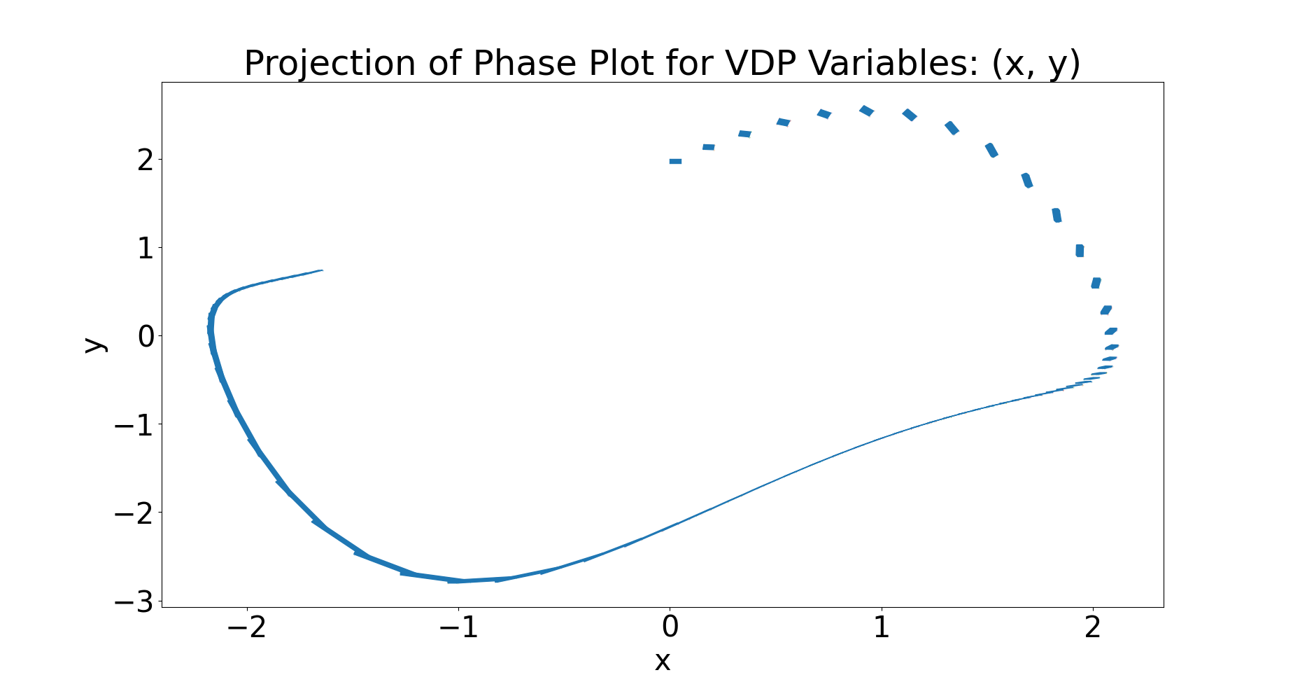
(a) 5 Lin

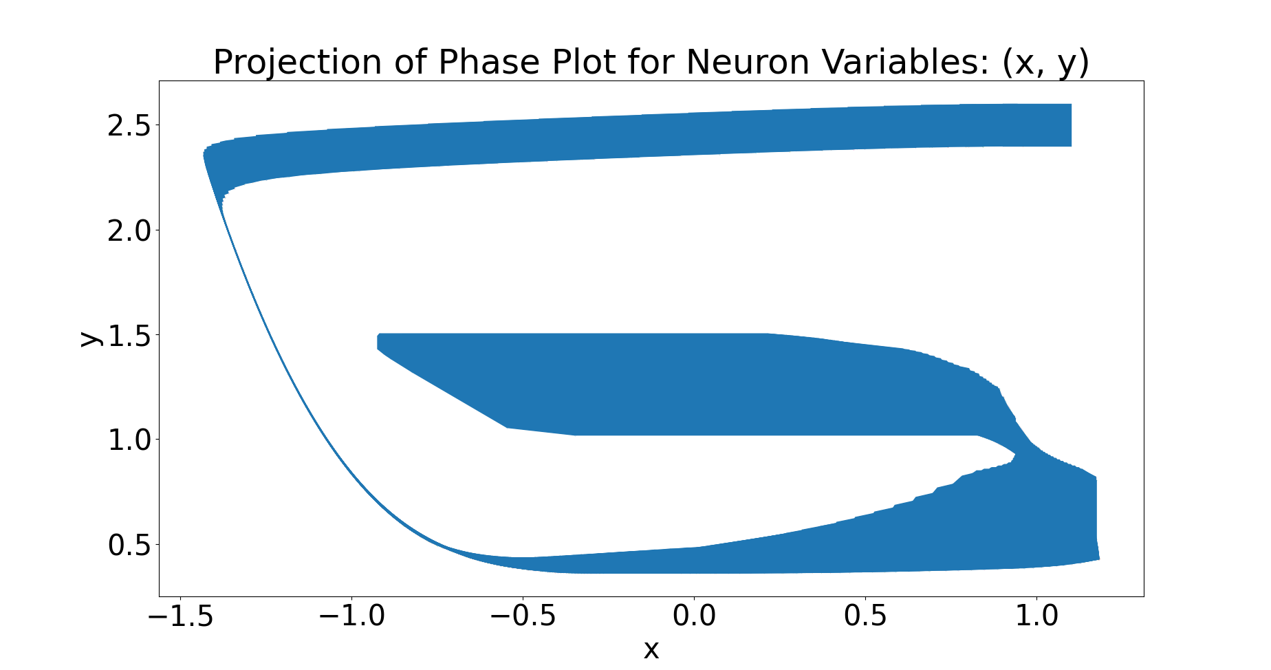
(b) 1 PCA 5 Lin

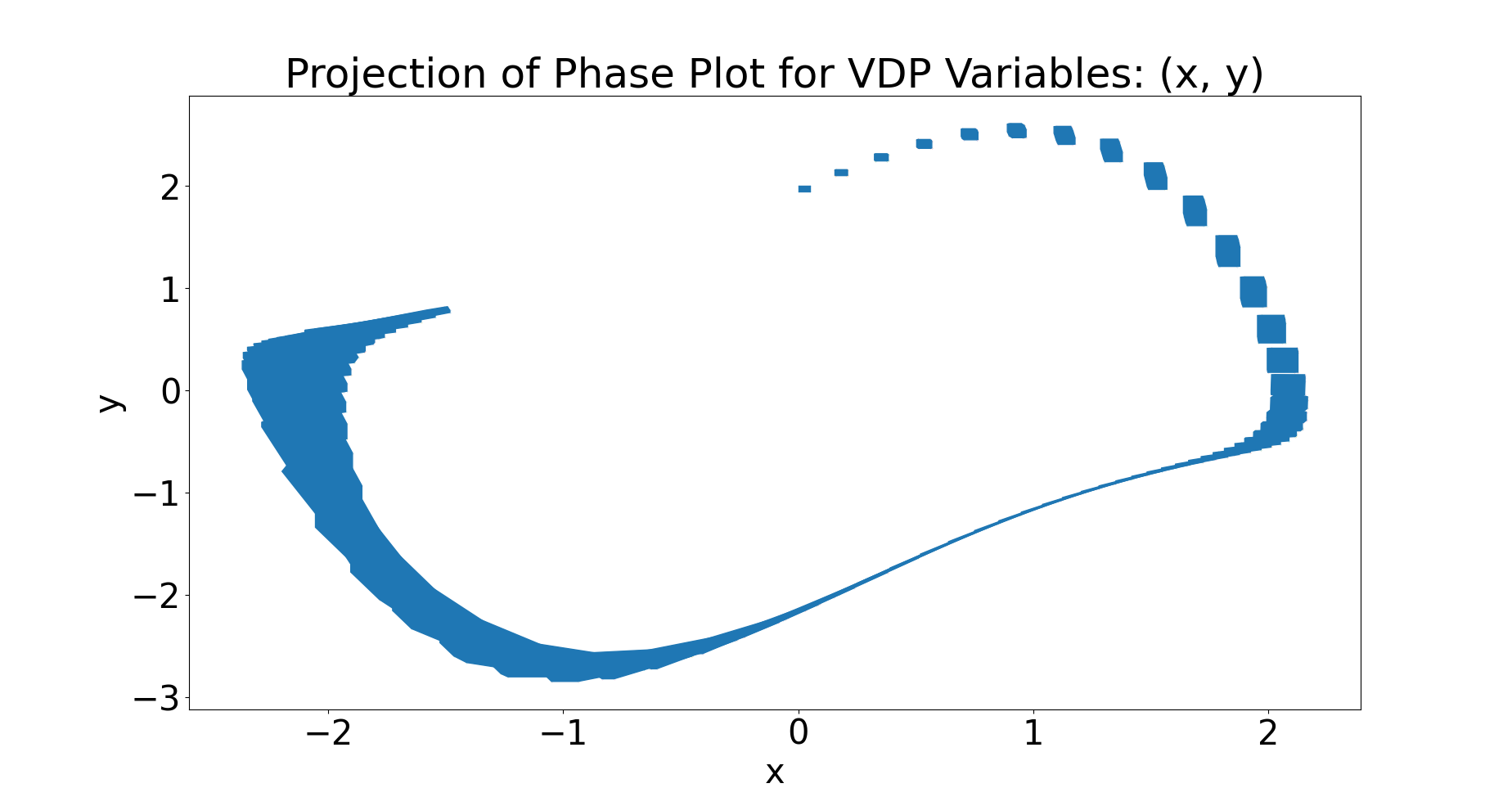
(c) 5 PCA

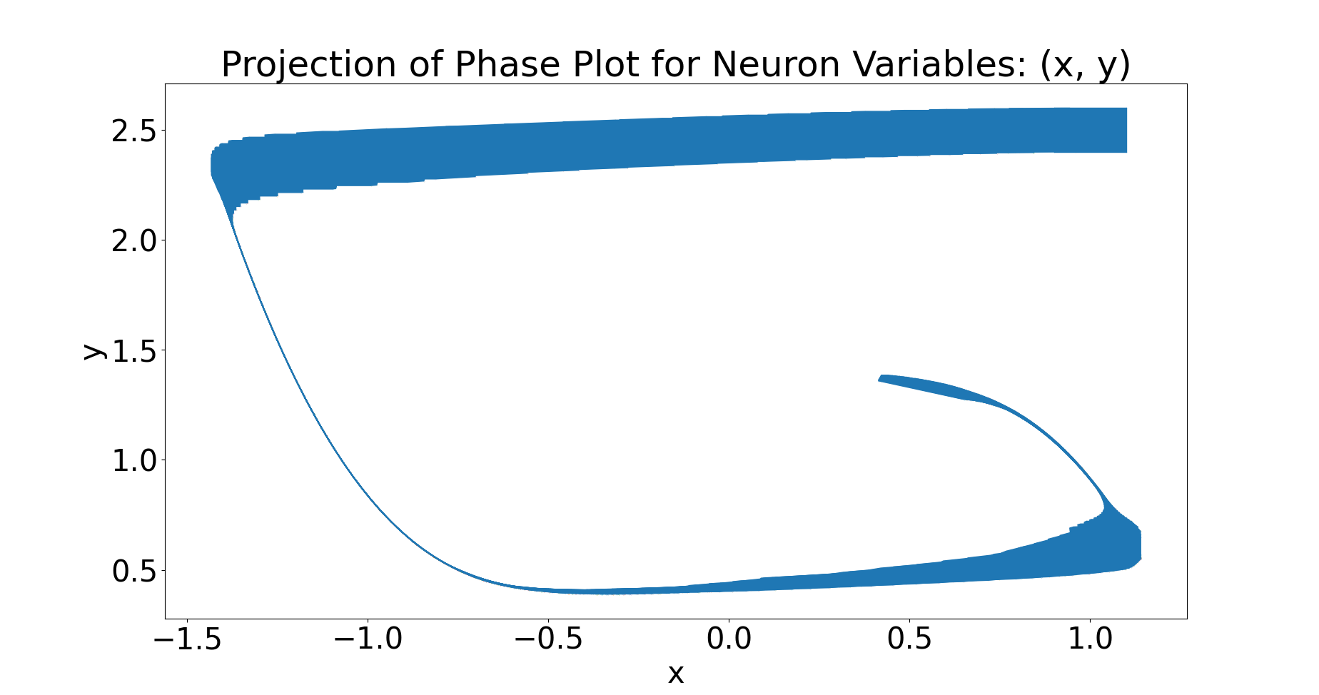
(d) 5 PCA 1 Lin

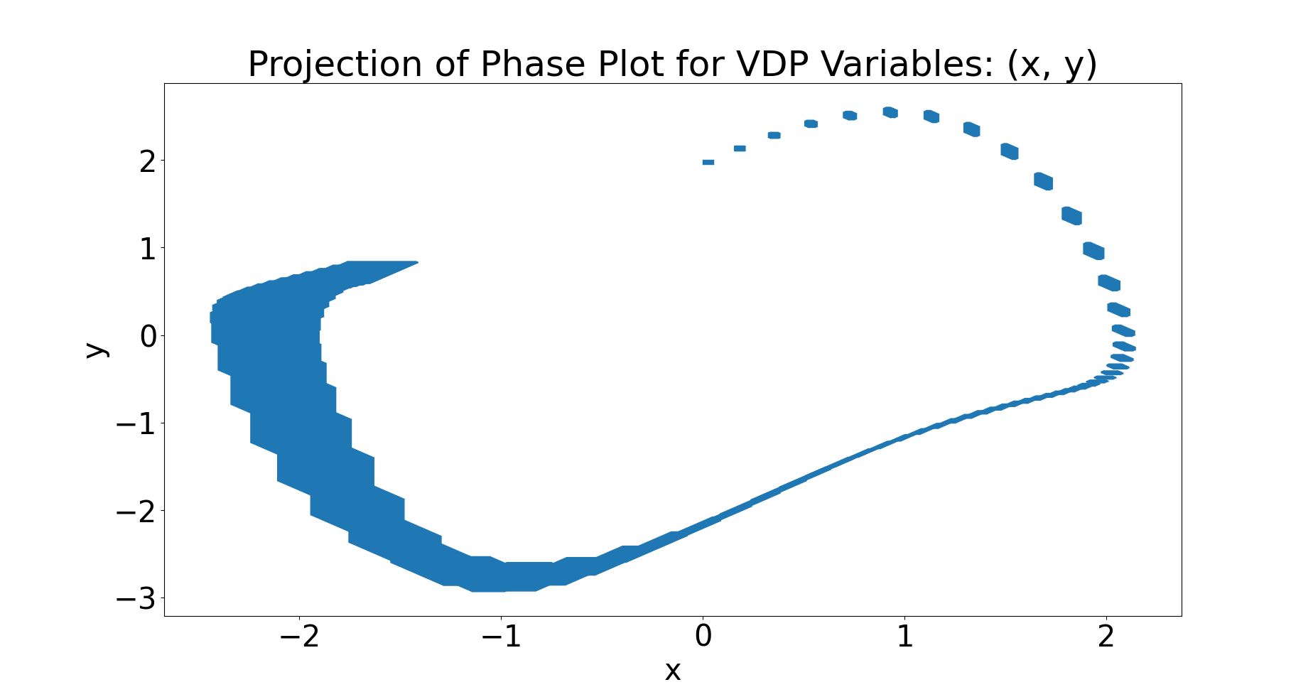
(e) Sapo

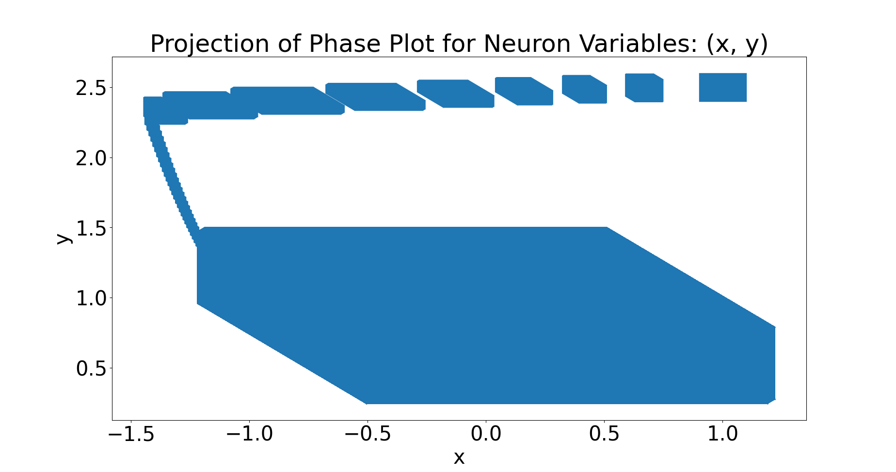
(f) Sapo

Figure 1: Effect of varying ratio between the number of PCA and Linear Approximation parallelotopes. The Vanderpol (left) and the FitzHugh-Nagumo Neuron (right) phase plots are shown to illustrate differing effects of varying the PCA/LinApp ratio. The initial set for the Vanderpol model is set to $x\in[0,0.05],\,y\in[1.95,2]$

5.0.3 Performance under Increasing Initial Sets

A key advantage of our dynamic strategies is the improved ability to control the wrapping error naturally arising from larger initial sets. Figure 2 presents charts showcasing the effect of increasing initial sets on the total flowpipe volume. We vary the initial box dimensions to gradually increase the box’s volume. We then plot the total flowpipe volume after running the benchmark. The same initial boxes are also used in computations using Sapo’s static parallelotopes. The number of parallelotopes defined by PCA and Linear Approximation directions were chosen based on best performance as seen in Table 2. We remark that our dynamic strategies perform better than static ones in controlling the total flowpipe volume as the initial set becomes larger. On the other hand, the performance of static parallelotopes tends to degrade rapidly as we increase the volume of the initial box.

5.0.4 Performance against Random Static Templates

We additionally benchmark our dynamic strategies against static random parallelotope bundles. We sample such parallelotopes in $n$ dimensions by first sampling a set of $n$ directions uniformly on the surface of the unit $(n-1)$-sphere, then defining our parallelotope using these sampled directions. We sample twenty of these parallelotopes for each trial and average the total flowpipe volumes. As shown in Figure 3, our best-performing dynamic strategies consistently outperform static random strategies for all tested benchmarks.

6 Conclusions

In this paper, we investigated two techniques for generating templates dynamically: first using linear approximation of the dynamics, and second using PCA. We demonstrated that these techniques improve the accuracy of reachable set by an order of magnitude when compared to static or random template directions. We also observed that both these techniques improve the accuracy of the reachable sets for different benchamrks. In future, we intend to investigate Koopman linearization techniques for computing alternative linear approximation template directions [4]. We also wish to investigate the use of a massively parallel implementation using HPC hardware such as GPUs for optimizing over an extremely large number of parallelotopes and their template directions. This is inspired by the approach behind the recent tool PIRK [11].

6.1 Acknowledgements

Parasara Sridhar Duggirala and Edward Kim acknowledge the support of the Air Force Office of Scientific Research under award number FA9550-19-1-0288 and FA9550-21-1-0121 and National Science Foundation (NSF) under grant numbers CNS 1935724 and CNS 2038960. Any opinions, findings, and conclusions or recommendations expressed in this material are those of the author(s) and do not necessarily reflect the views of the United States Air Force or the National Science Foundation.

Strategy	Total Volume
5 LinApp	0.227911
1 PCA, 4 LinApp	0.225917
2 PCA, 3 LinApp	0.195573
3 PCA, 2 LinApp	0.188873
4 PCA, 1 LinApp	1.227753
5 PCA	1.509897
5 Static Diagonal(Sapo)	2.863307

(a) Vanderpol

Strategy	Total Volume
5 LinApp	58199.62
1 PCA, 4 LinApp	31486.16
2 PCA, 3 LinApp	5204.09
3 PCA, 2 LinApp	6681.76
4 PCA, 1 LinApp	50505.10
5 PCA	84191.15
5 Static Diagonal (Sapo)	66182.18

(b) Jet Engine

Strategy	Total Volume
5 LinApp	154.078
1 PCA, 4 LinApp	136.089
2 PCA, 3 LinApp	73.420
3 PCA , 2 LinApp	73.126
4 PCA, 1 LinApp	76.33
5 PCA	83.896
5 Static Diagonal (Sapo)	202.406

(c) FitzHugh-Nagumo

Strategy	Total Volume
2 LinApp	0.001423
1 PCA, 1 LinApp	0.106546
2 PCA	0.117347
2 Static Diagonal (Sapo)	0.020894

(d) SIR

Strategy	Total Volume
5 LinApp	5.5171
1 PCA, 4 LinApp	5.2536
2 PCA, 3 LinApp	5.6670
3 PCA, 2 LinApp	5.5824
4 PCA, 1 LinApp	312.2108
5 PCA	388.0513
5 Static Diagonal (Best)	3023.4463

(e) Coupled Vanderpol

Strategy	Total Volume
3 LinApp	$2.95582227*10^{-10}$
1 PCA, 2 LinApp	$2.33007583*10^{-10}$
2 PCA, 1 LinApp	$4.02751770*10^{-9}$
3 PCA	$4.02749571*10^{-9}$
3 Static Diagonal (Sapo)	$4.02749571*10^{-9}$

(f) COVID

Table 2: Tables presenting upper bounds on the total reachable set volume by strategy. The static directions are retrieved and/or inspired from Sapo models of equal dimension for benchmarking. The best performing strategy is highlighted in bold.

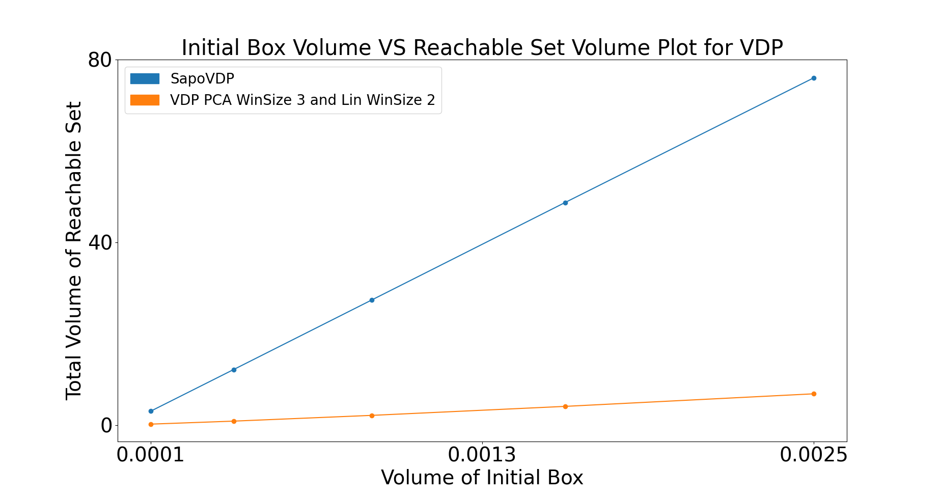
(a) Vanderpol

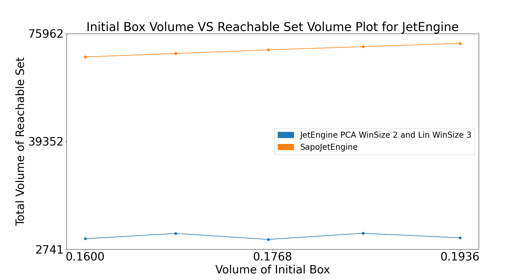
(b) Jet Engine

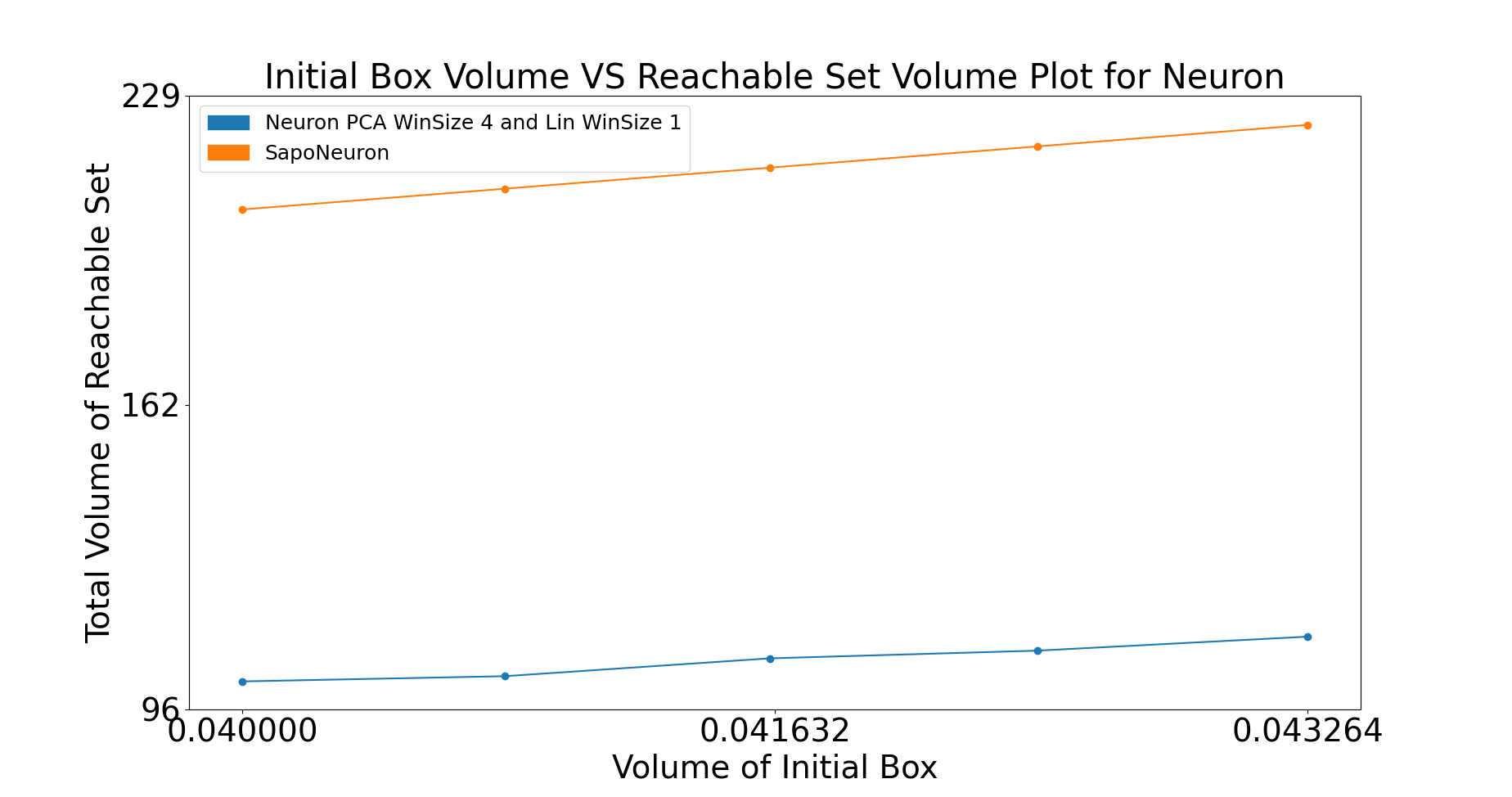
(c) Neuron

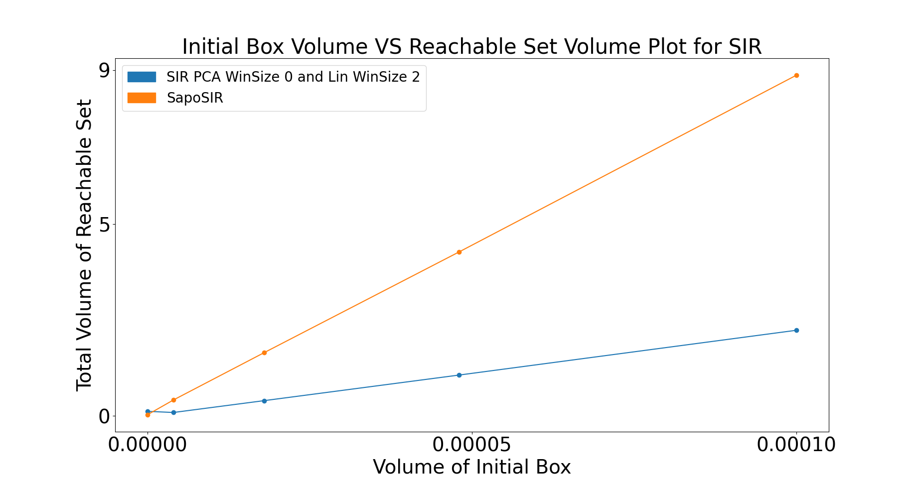
(d) SIR

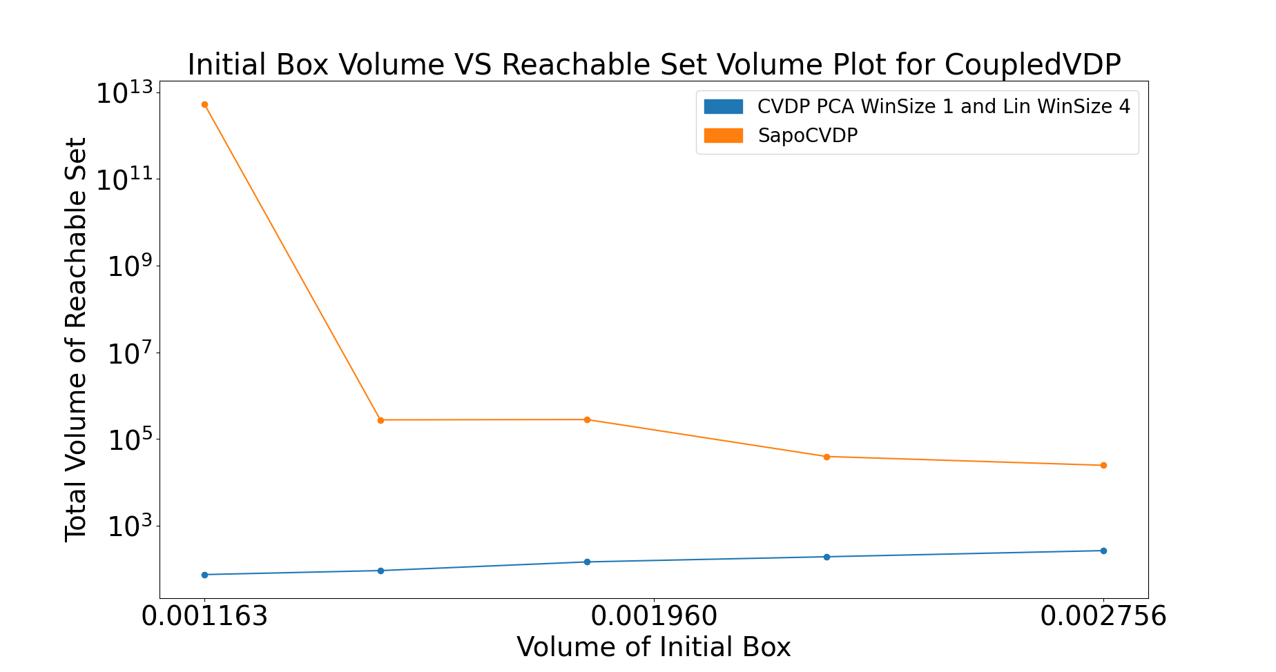
(e) Coupled Vanderpol

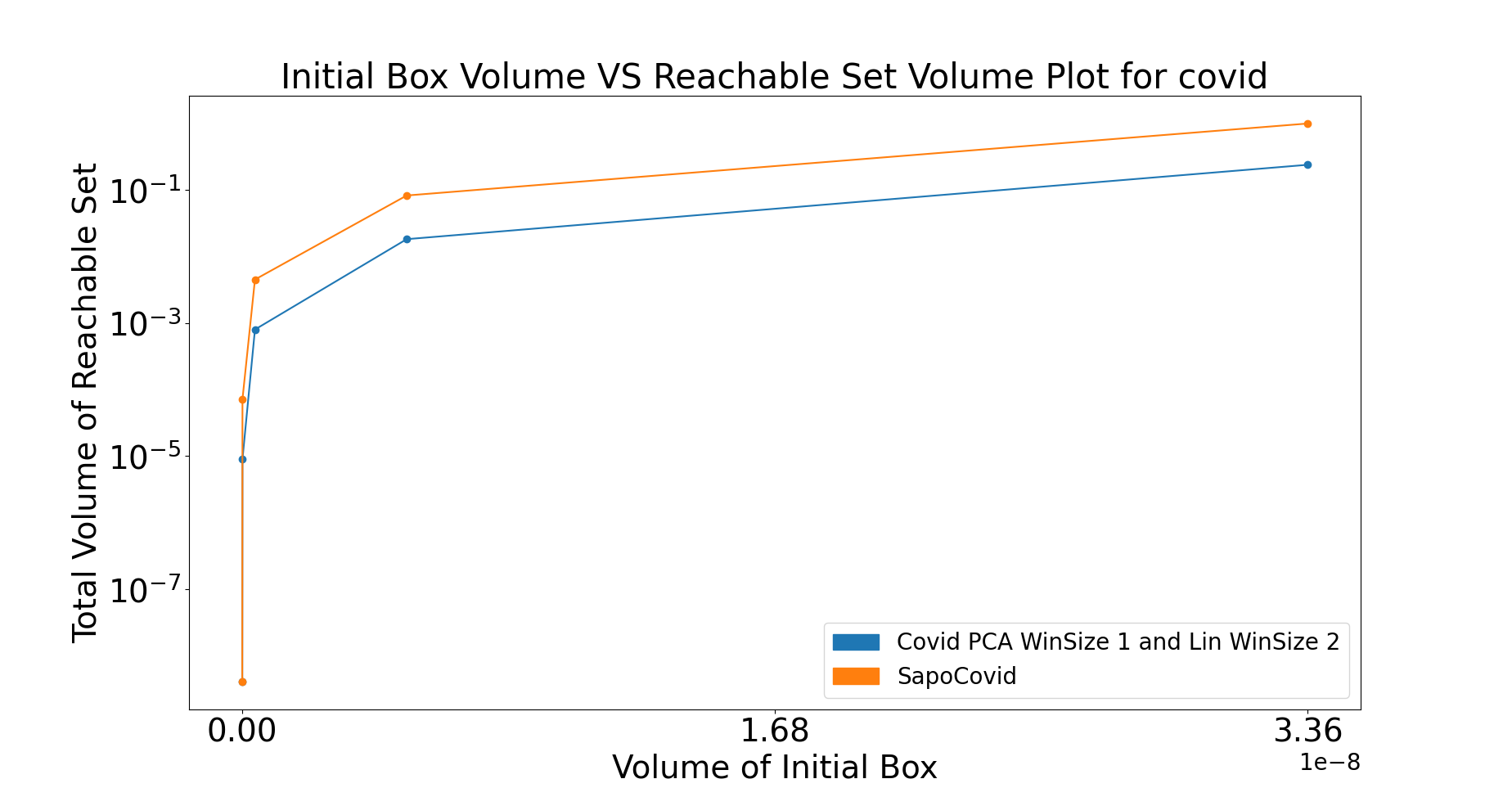
(f) COVID

Figure 2: Comparison between the performance of diagonal static parallelotope bundles and that of the best performing dynamic parallelotope bundles as the volume of the initial set grows.

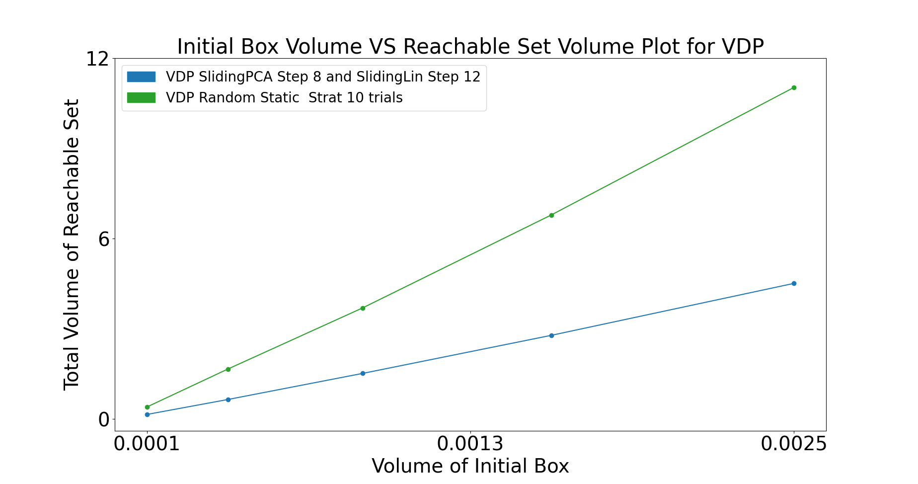
(a) Vanderpol

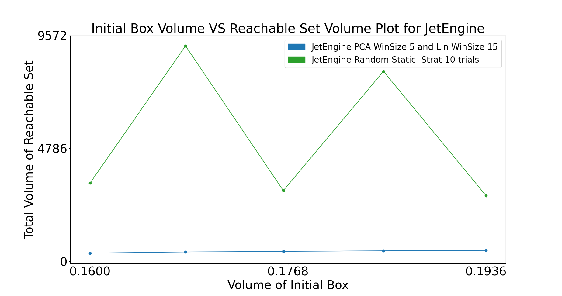
(b) Jet Engine

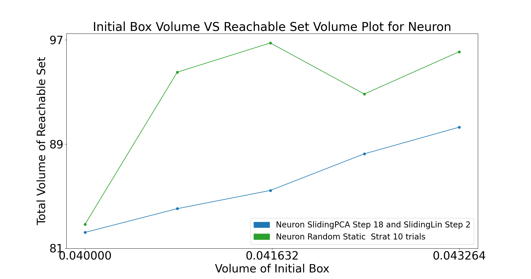
(c) Neuron

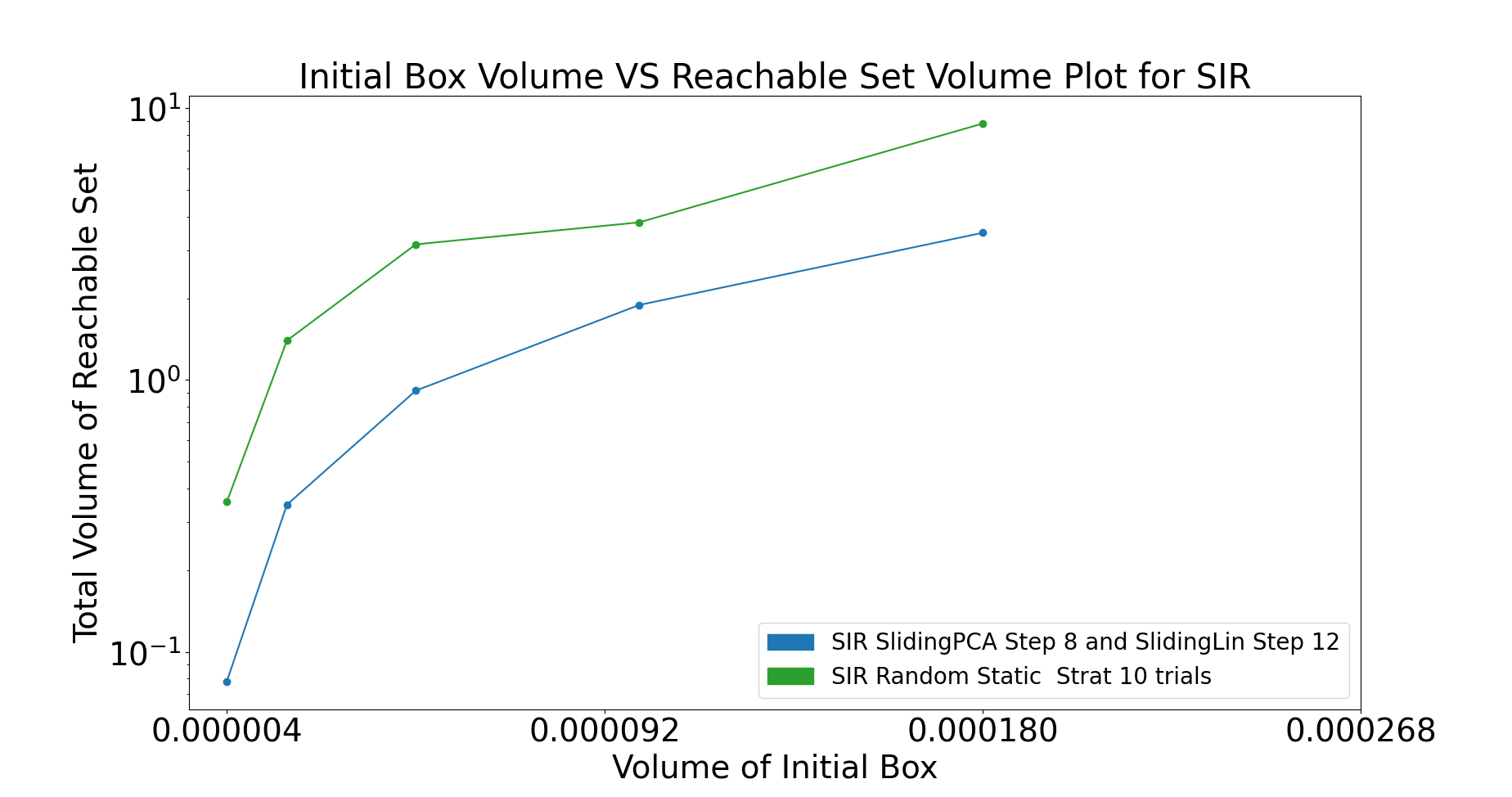
(d) SIR

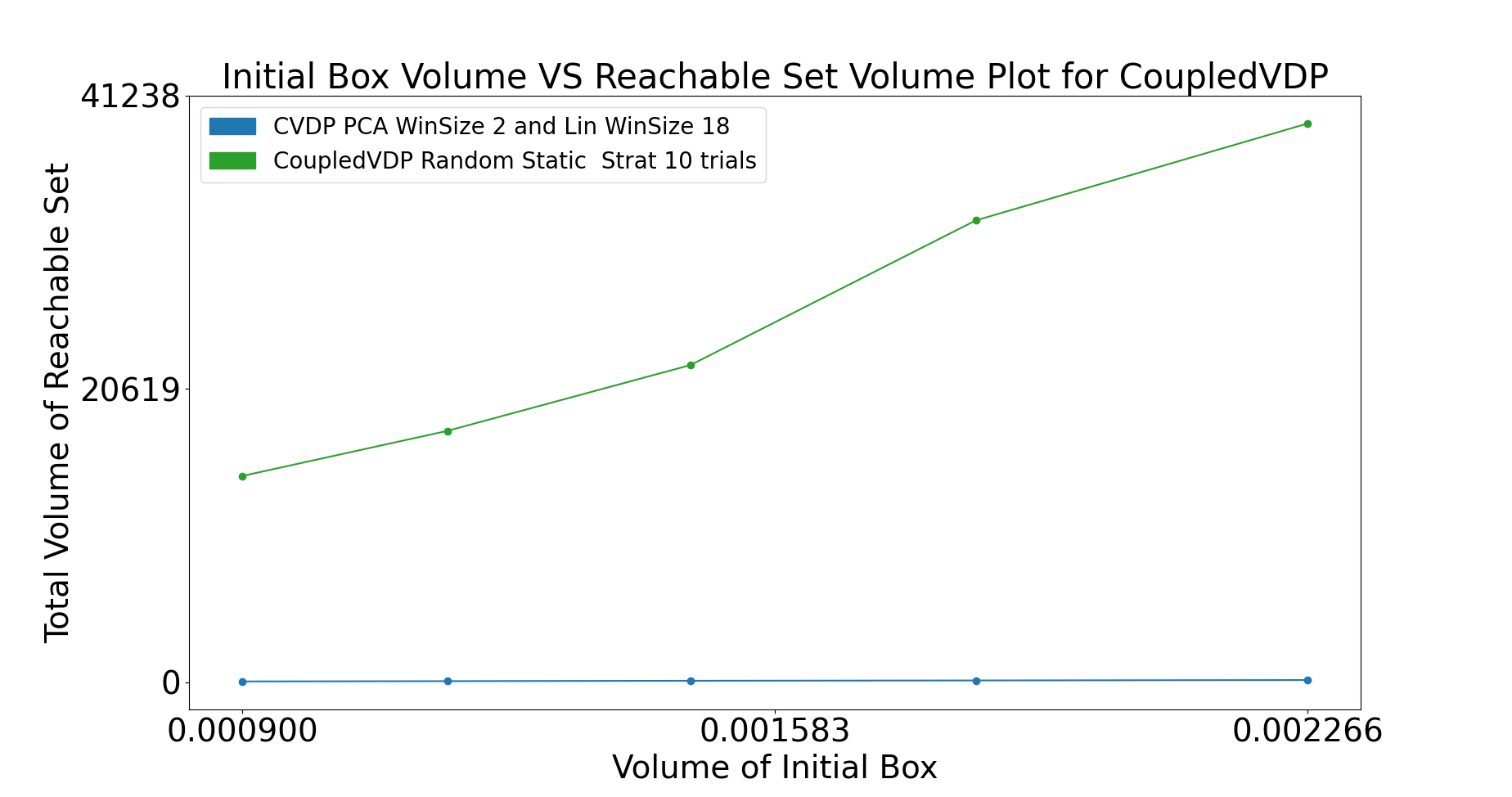
(e) Coupled Vanderpol

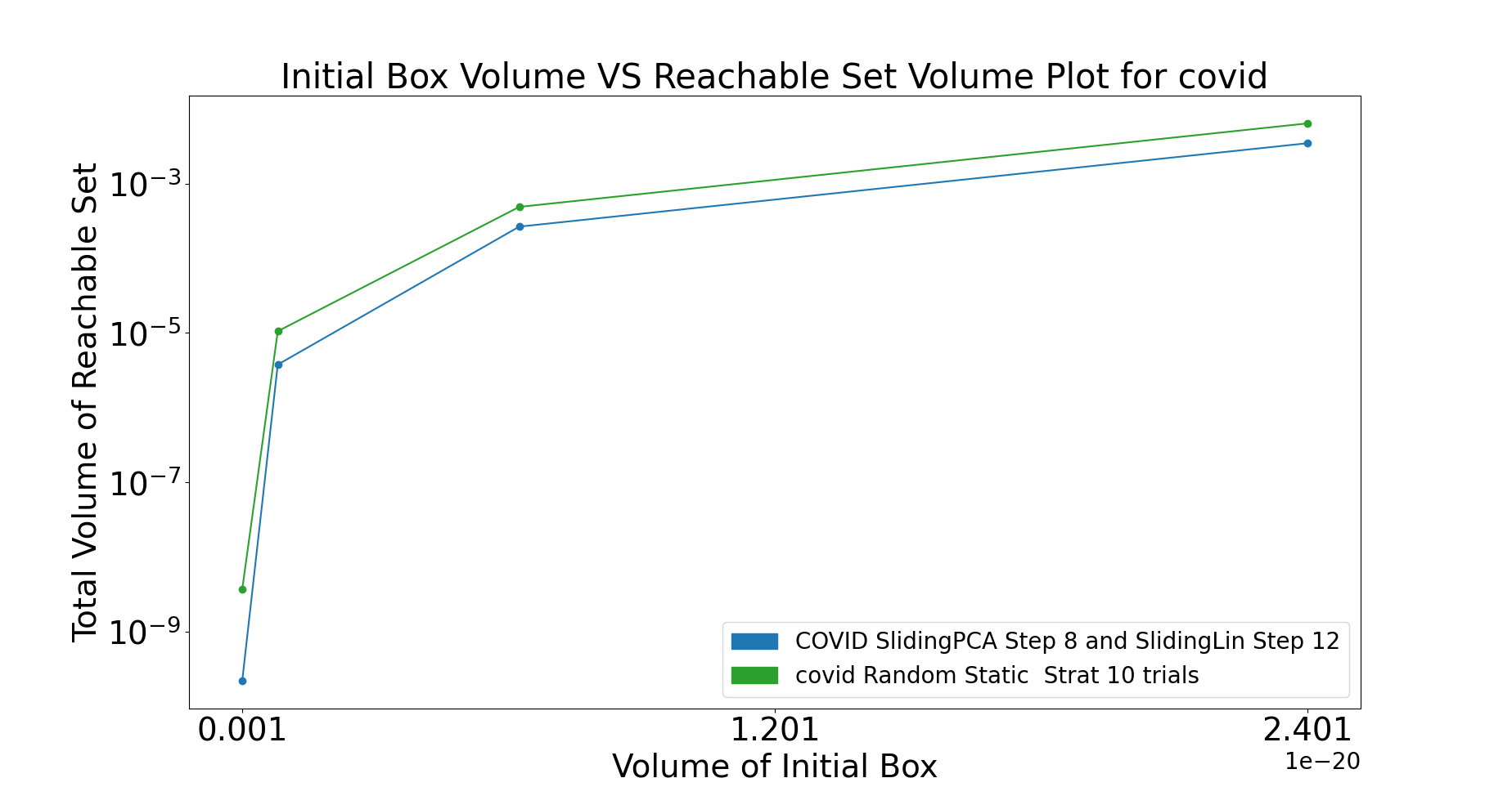
(f) COVID

Figure 3: Comparision between random static strategies and the best performing dynamic strategies as the volume of the initial set grows. The total reachable set volumes for random static strategies are averaged over ten trials for each system.

References

- [1] Kodiak, a C++ library for rigorous branch and bound computation. https://github.com/nasa/Kodiak, Accessed: July 2020.
- [2] M. Althoff, O. Stursberg, and M. Buss. Computing reachable sets of hybrid systems using a combination of zonotopes and polytopes. Nonlinear analysis: hybrid systems, 4(2):233–249, 2010.
- [3] S. Ansumali, S. Kaushal, A. Kumar, M. K. Prakash, and M. Vidyasagar. Modelling a pandemic with asymptomatic patients, impact of lockdown and herd immunity, with applications to sars-cov-2. Annual Reviews in Control, 2020.
- [4] S. Bak, S. Bogomolov, P. S. Duggirala, A. R. Gerlach, and K. Potomkin. Reachability of black-box nonlinear systems after Koopman operator linearization, 2021.
- [5] X. Chen and E. Ábrahám. Choice of directions for the approximation of reachable sets for hybrid systems. In International Conference on Computer Aided Systems Theory, pages 535–542. Springer, 2011.
- [6] R. Clarisó and J. Cortadella. The octahedron abstract domain. In International Static Analysis Symposium, pages 312–327. Springer, 2004.
- [7] T. Dang, T. Dreossi, and C. Piazza. Parameter synthesis using parallelotopic enclosure and applications to epidemic models. In International Workshop on Hybrid Systems Biology, pages 67–82. Springer, 2014.
- [8] T. Dang and T. M. Gawlitza. Template-based unbounded time verification of affine hybrid automata. In Asian Symposium on Programming Languages and Systems, pages 34–49. Springer, 2011.
- [9] T. Dang and D. Salinas. Image computation for polynomial dynamical systems using the Bernstein expansion. In International Conference on Computer Aided Verification, pages 219–232. Springer, 2009.
- [10] T. Dang and R. Testylier. Reachability analysis for polynomial dynamical systems using the Bernstein expansion. Reliable Computing, 17(2):128–152, 2012.
- [11] A. Devonport, M. Khaled, M. Arcak, and M. Zamani. PIRK: Scalable interval reachability analysis for high-dimensional nonlinear systems. In International Conference on Computer Aided Verification, pages 556–568. Springer, 2020.
- [12] T. Dreossi. Sapo: Reachability computation and parameter synthesis of polynomial dynamical systems. In Proceedings of the 20th International Conference on Hybrid Systems: Computation and Control, pages 29–34, 2017.
- [13] T. Dreossi, T. Dang, and C. Piazza. Parallelotope bundles for polynomial reachability. In Proceedings of the 19th International Conference on Hybrid Systems: Computation and Control, pages 297–306, 2016.
- [14] T. Dreossi, T. Dang, and C. Piazza. Reachability computation for polynomial dynamical systems. Formal Methods in System Design, 50(1):1–38, 2017.
- [15] P. S. Duggirala and M. Viswanathan. Parsimonious, simulation based verification of linear systems. In International Conference on Computer Aided Verification, pages 477–494. Springer, 2016.
- [16] R. FitzHugh. Impulses and physiological states in theoretical models of nerve membrane. Biophysical journal, 1(6):445–466, 1961.
- [17] J. Garloff. The Bernstein expansion and its applications. Journal of the American Romanian Academy, 25:27, 2003.
- [18] A. Girard. Reachability of uncertain linear systems using zonotopes. In International Workshop on Hybrid Systems: Computation and Control, pages 291–305. Springer, 2005.
- [19] J. Gronski, M.-A. B. Sassi, S. Becker, and S. Sankaranarayanan. Template polyhedra and bilinear optimization. Formal Methods in System Design, 54(1):27–63, 2019.
- [20] C. Huang, J. Fan, W. Li, X. Chen, and Q. Zhu. Reachnn: Reachability analysis of neural-network controlled systems. ACM Transactions on Embedded Computing Systems (TECS), 18(5s):1–22, 2019.
- [21] E. Kim and P. S. Duggirala. Kaa: A Python implementation of reachable set computation using Bernstein polynomials. EPiC Series in Computing, 74:184–196, 2020.
- [22] C. Muñoz and A. Narkawicz. Formalization of Bernstein polynomials and applications to global optimization. Journal of Automated Reasoning, 51(2):151–196, 2013.
- [23] P. S. Nataraj and M. Arounassalame. A new subdivision algorithm for the Bernstein polynomial approach to global optimization. International journal of automation and computing, 4(4):342–352, 2007.
- [24] P. Nataray and K. Kotecha. An algorithm for global optimization using the Taylor–Bernstein form as inclusion function. Journal of Global Optimization, 24(4):417–436, 2002.
- [25] National Supermodel Committee . Indian Supermodel for Covid-19 Pandemic.
- [26] S. Sankaranarayanan, T. Dang, and F. Ivančić. Symbolic model checking of hybrid systems using template polyhedra. In International Conference on Tools and Algorithms for the Construction and Analysis of Systems, pages 188–202. Springer, 2008.
- [27] M. A. B. Sassi, R. Testylier, T. Dang, and A. Girard. Reachability analysis of polynomial systems using linear programming relaxations. In International Symposium on Automated Technology for Verification and Analysis, pages 137–151. Springer, 2012.
- [28] Y. Seladji. Finding relevant templates via the principal component analysis. In International Conference on Verification, Model Checking, and Abstract Interpretation, pages 483–499. Springer, 2017.
- [29] A. P. Smith. Fast construction of constant bound functions for sparse polynomials. Journal of Global Optimization, 43(2-3):445–458, 2009.
- [30] O. Stursberg and B. H. Krogh. Efficient representation and computation of reachable sets for hybrid systems. In International Workshop on Hybrid Systems: Computation and Control, pages 482–497. Springer, 2003.