Guaranteed a posteriori local error estimation for finite element solutions of boundary value problems

Abstract

This paper considers the finite element solution of the boundary value problem of Poisson’s equation and proposes a guaranteed a posteriori local error estimation based on the hypercircle method. Compared to the existing literature on qualitative error estimation, the proposed error estimation provides an explicit and sharp bound for the approximation error in the subdomain of interest, and its efficiency can be enhanced by further utilizing a non-uniform mesh. Such a result is applicable to problems without $H^{2}$-regularity, since it only utilizes the first order derivative of the solution. The efficiency of the proposed method is demonstrated by numerical experiments for both convex and non-convex 2D domains with uniform or non-uniform meshes.

65N15, 65N30

1 Introduction

This paper studies the finite element solution of the boundary value problem (BVP) of Poisson’s equation, and proposes an a posteriori local error estimation method for finite element solution, based on the hypercircle method, i.e., the Prager–Synge theorem.

The motivation of this research originates from the error analysis of the four-probe method, which has been used for the resistivity measurement of semiconductors over the past century [7]. The image of the four-probe method is illustrated in Figure 1: four probes $A,B,C$, and $D$ are aligned on the surface of the sample; a constant current $I_{AD}$ is applied between $A$ and $D$ and the potential difference $V_{BC}$ between $B$ and $C$ is measured. The resistivity $\rho$ is then calculated by $\rho=F_{c}V_{BC}/I_{AD}$, where $F_{c}$ is the correction factor. As an important quantity for high-precision measurement, $F_{c}$ is evaluated theoretically by considering the governing equation of the distribution of the potential. A well-used model for the potential distribution $u$ is described by the following boundary value problem of Poisson’s equation (see, e.g., [7, 27]):

(1) $$-\Delta u=2\rho\>I_{AD}\>(\delta(A;x)-\delta(D;x))\mbox{ in }\Omega;\quad\frac{\partial u}{\partial\mathbf{n}}=0\mbox{ on }\partial\Omega\>,$$

where $\delta(A;x)$ and $\delta(D;x)$ are Dirac’s delta functions located at $A$ and $D$, respectively. Note that this model regards the current $I_{AD}$ as a point charge on the surface of the sample. By setting $\rho\>I_{AD}=1$, the value of $F_{c}$ can be evaluated by

$$F_{c}=\frac{1}{u(B)-u(C)}\>.$$

The calculation of $F_{c}$ only utilizes the potential $u$ at the probes $B$ and $C$, i.e., the local information of the solution around the probes. To have a sharp estimation of the correction factor $F_{c}$, the local error around the probes is of interest and the local error estimation for the FEM approximation to $u$ is wanted. Note that the right-hand side of (1) does not belong to the $L^{2}$ space. In this study, instead of the equation (1), a model problem $-\Delta u=f$ with $f\in L^{2}(\Omega)$ is considered. The technique to solve equation (1) directly will be discussed in our subsequent papers.

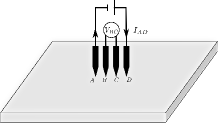
Figure 1: The four-probe method

There is some literature related on local error estimation for finite element solutions (see, e.g.,[18, 23, 25, 14, 5, 3, 4, 24, 21, 22]). The local error estimation was first studied by Nitche and Schatz in [18]. In the studies of [18, 23], for the subdomain $\Omega_{0}$ of interest, an intermediate subdomain $\Omega_{1}$ such that $\Omega_{0}\subset\joinrel\subset\Omega_{1}\subset\joinrel\subset\Omega$ is utilized to deduce the following error estimation: for $u\in H^{l}(\Omega)$,

$$\|u-u_{h}\|_{s,\Omega_{0}}\leq C(h^{l-s}\|u\|_{l,\Omega_{1}}+\|u-u_{h}\|_{-p,\Omega_{1}})\>,$$

for $s=0$ or $1$ and $p$ as a fixed integer. In [18] , an estimation for quasi-uniform meshes was provided. In [25, 26], based on the knowledge of the local error distribution, Xu and Zhou purposed a parallel technique that uses coarse grid to approximate the low frequencies part of the residual error and then uses fine grid for the high frequency part. Discussions on relaxing the assumption in [18] applied to the mesh can be found in [5, 2]. In the field of adaptive finite element methods, error indicators based on the local error estimation have been well studied; see, e.g.,[25, 26, 14, 3, 4].

The above results on local error estimation mainly focus on the qualitative analysis (e.g., convergence rate) of local error terms, while the explicit bound for the local error estimation is not available.

In this paper, we propose a quantitative error estimation method for the local error of the finite element solutions. Such a method is regarded as an extension of the explicit error estimation theorem developed by Liu [15], which inherits the idea of Kikuchi [11] to utilize the hypercircle method. The idea of local error estimation was also introduced in a concise manner in our previous work [16] published in Japanese. Here, thorough discussions along with detailed numerical examples are provided to describe this newly developed local error estimation method.

The application of the hypercircle method to the a posteriori error estimation can also be found in [1, 17]. Instead of developing $\mathbf{p}_{h}\in H(\mbox{div\>};\Omega)$ by processing the discontinuity of $\nabla u_{h}$ across the edges of elements [1, 17], the feature of Kikuchi’s approach and our method is to construct the hypercircle by utilizing $\mathbf{p}_{h}\in H(\mbox{div\>};\Omega)$ such that $\mbox{div\>}{\mathbf{p}}_{h}+f_{h}=0$ holds exactly, where $f_{h}$ is the projection of $f$ to totally discontinuous piecewise polynomials.

The hypercircle method, namely the Prager–Synge theorem, was developed more than fifty years ago by [20] for elastic analysis. Around the same time [20], based on the $T^{*}T$ theory of Kato [8], Fujita developed a method similar to the hypercircle method [6], which has been applied to develop the point-wise estimation method for boundary value problems with specially constructed base functions. The extension of Kato–Fujita’s approach to finite element method for local error estimation will be considered in our succeeding work.

The local error estimation proposed in this paper has the following features.

• As a quantitative result, it provides explicit estimation for the energy error in the subdomain of interest.

• The method deals with domains of general shapes in the natural way and is applicable to non-convex domains where a singularity may appear around the re-entry corner of the boundary.

• There are no constraints on the mesh generation of the domain, compared to the stringent requirement of a uniform mesh in past studies on local error estimation. Also, the proposed local error estimator has an optimal convergence rate for the finite element solutions when non-uniform meshes are utilized to obtain finer solution approximation over the subdomain of interest.

The rest of the paper is organized as follows: In section 2, we provide preliminary information on the problem setting and basic knowledge about the finite element method spaces. In section 3, the global error estimation based on the hypercircle method developed in [15] is introduced. In section 4, the details of the local error estimation are described. In section 5, the qualitative analysis about the convergence rate of the proposed local error estimation is discussed. In section 6, the numerical examples for Poisson’s equation over the square domain and the L-shaped domain are presented. Finally, in section 7, we summarize the conclusions and discuss future studies.

2 Preliminary

2.1 Problem settings

Throughout this study, the domain $\Omega$ is assumed to be a bounded polygonal domain of $\mathbb{R}^{2}$. Thus, $\Omega$ can be completely triangulated without any gap near the boundary. Standard symbols are used for the Sobolev spaces $H^{m}(\Omega)(m>0)$. The norm of $L^{2}(\Omega)$ is written as $\|\cdot\|_{L^{2}(\Omega)}$ or $\|\cdot\|_{\Omega}$ . Symbols $|\cdot|_{H^{m}(\Omega)},\|\cdot\|_{H^{m}(\Omega)}$ denote semi-norm and norm of $H^{m}(\Omega)$, respectively. Let $(\cdot,\cdot)$ be the inner product of $L^{2}(\Omega)$ or $(L^{2}(\Omega))^{2}$. Sobolev space $W^{1,\infty}(\Omega)$ is a function space where weak derivatives up to the first order are essentially bounded on $\Omega$. The standard vector valued function space $H(\mbox{div};\Omega)$ is defined as follows:

$$H(\mbox{div};\Omega):=\left\{\mathbf{q}\in(L^{2}(\Omega))^{2};~{}\mbox{div }\mathbf{q}\in L^{2}(\Omega)\right\}.$$

In this paper, the finite element solution for the following model boundary value problem will be discussed:

(2) $$-\Delta u=f\mbox{ in }\Omega,\quad\displaystyle\frac{\partial u}{\partial\mathbf{n}}=g_{N}\mbox{ on }\Gamma_{N},\quad u=g_{D}\mbox{ on }\Gamma_{D}.$$

Here, $\Gamma_{N}$ and $\Gamma_{D}$ are disjoint subsets of $\partial\Omega$ satisfying $\Gamma_{N}\cup\Gamma_{D}=\partial\Omega$; $\mathbf{n}$ is the unit outer normal direction on the boundary and $\frac{\partial}{\partial\mathbf{n}}$ is the directional derivative along $\mathbf{n}$ on $\partial\Omega$.

Let $S$ be a subdomain of $\Omega$ of interest. Suppose that $u_{h}$ is an approximate solution to the problem (2). The error of $(\nabla u-\nabla u_{h})$ in the subdomain $S$ will be evaluated in this study.

The weak form for the aforementioned problem is given by:

(3) $$\mbox{Find }u\in V\mbox{ s.t. }(\nabla u,\nabla v)=(f,v)+(g_{N},v)_{\Gamma_{N}},\quad\forall v\in V_{0}.$$

where

$$(g_{N},v)_{\Gamma_{N}}:=\int_{\Gamma_{N}}g_{N}v~{}ds.$$

In case $\Gamma_{D}$ is not an empty set, the function space $V$ of the trial function and the function space $V_{0}$ of the test function are defined by

$$V:=\left\{v\in H^{1}(\Omega);v=g_{D}\mbox{ on }\Gamma_{D}\right\},~{}V_{0}:=\left\{v\in H^{1}(\Omega);v=0\mbox{ on }\Gamma_{D}\right\}.$$

For an empty $\Gamma_{D}$, the definition of $V$ and $V_{0}$ are modified as follows:

$$V=V_{0}=\left\{v\in H^{1}(\Omega);\int_{\Omega}v~{}dx=0\right\}.$$

2.2 Finite element space setting

To prepare for the discussion on the newly developed local error estimation in §4, we review the standard FEM approaches to (2). To simplify the discussion, assume $g_{D},g_{N}$ in the boundary conditions of the model problem (2) to be piecewise linear and piecewise constant at the boundary edges of $\mathcal{T}^{h}$, respectively. Let $\mathcal{T}_{h}$ be a proper triangulation of the domain $\Omega$. Given an element $K\in\mathcal{T}_{h}$, let $h_{K}$ denote the length of longest edge of $K$. The mesh size $h$ of $\mathcal{T}_{h}$ is defined as follows:

$$h:=\max_{K\in\mathcal{T}_{h}}h_{K}.$$

On each element $K\in\mathcal{T}_{h}$, the set of polynomials with degree up to $d$ is denoted by $P_{d}(K)$. Let $V_{h},V_{h,0}$ denote the finite element spaces consisting of piecewise linear and continuous functions, the boundary conditions of which follow the settings of $V$ and $V_{0}$, respectively. The conforming finite element formulation of (3) is given by

(4) $$\mbox{Find }u_{h}\in V_{h}\mbox{ s.t. }(\nabla u_{h},\nabla v_{h})=(f,v_{h})+(g_{N},v_{h})_{\Gamma_{N}},\quad\forall v_{h}\in V_{h,0}.$$

To provide the local error estimation for $(\nabla u-\nabla u_{h})$ over the subdomain $S$, let us introduce the following finite element spaces.

• Piecewise constant function space:

  $$X_{h}:=\left\{v_{h}\in L^{2}(\Omega)~{}:~{}v_{h}|_{K}\in P_{0}(K),~{}\forall K\in\mathcal{T}_{h}\right\}.$$

  In case $\Gamma_{D}$ is empty, it is further required that $\int_{\Omega}vdx=0$ for $v_{h}\in X_{h}$.

• The Raviart–Thomas finite element space:

  $$RT_{h}:=\left\{\mathbf{p}_{h}\in H(\mbox{div};\Omega)~{}:~{}\mathbf{p}_{h}|_{K}=(a_{K}+c_{K}x,b_{K}+c_{K}y)\mbox{ for }K\in\mathcal{T}_{h}\right\}.$$

  $$RT_{h,0}=\{\mathbf{p}_{h}\in RT_{h}~{}:~{}\mathbf{p}_{h}\cdot\mathbf{n}=0\mbox{ on }\Gamma_{N}\}\;.$$

  Here, $a_{K},b_{K},c_{K}\in P_{0}(K)$ for $K\in\mathcal{T}_{h}$.

The standard mixed finite element formulation of (2) reads: Find $(\mathbf{p}_{h},\mu_{h})\in RT_{h}\times X_{h},~{}\mathbf{p}_{h}\cdot\mathbf{n}=g_{N}\mbox{ on }\Gamma_{N}$, s.t.

(5) $$(\mathbf{p}_{h},\mathbf{q}_{h})+(\mbox{div }\mathbf{q}_{h},\mu_{h})+(\mbox{div }\mathbf{p}_{h},\eta_{h})=\int_{\Gamma_{D}}g_{D}(\mathbf{q}_{h}\cdot\mathbf{n})~{}ds-(f,\eta_{h})\;,$$

for $(\mathbf{q}_{h},\eta_{h})\in RT_{h,0}\times X_{h}$.

Define the projection $\pi_{h}:L^{2}(\Omega)\to X_{h}$ such that for $f\in L^{2}(\Omega)$,

$$(f-\pi_{h}f,\eta_{h})=0,\quad\forall\eta_{h}\in X_{h}.$$

The following error estimation holds for $\pi_{h}$,

(6) $$\|f-\pi_{h}f\|_{\Omega}\leq C_{0}h|f|_{H^{1}(\Omega)},\quad\forall f\in H^{1}(\Omega).$$

To give a concrete value of $C_{0}$ in (6), let us define $C_{0}(K)$ as a constant that depends on the shape of the triangle $K\in\mathcal{T}_{h}$ and satisfies

$$\|f-\pi_{h}f\|_{K}\leq C_{0}(K)|f|_{H^{1}(K)},\quad\forall f\in H^{1}(K).$$

By using $C_{0}(K)$, the constant $C_{0}$ that depends on triangulation can be defined by

(7) $$C_{0}:=\max_{K\in\mathcal{T}_{h}}\frac{C_{0}(K)}{h}.$$

The previous studies [9, 10, 12] reported that the optimal value of $C_{0}(K)$ is given by $C_{0}(K):=h_{K}/j_{1,1}(\leq 0.261h_{K})$ using positive minimum root $j_{1,1}\approx 3.83171$ of the first kind Bessel’s function $J_{1}$.

3 Global a priori error estimation for the finite element solutions

In this section, we introduce the global error estimation developed in [15, 19, 13], which will be used in Theorem 4.10 for local error estimation. We focus on the global a priori error estimation for problems with homogeneous boundary value conditions, which fits the needs in the proof for Theorem 4.10. For global a priori error estimation of non-homogeneous boundary value problems, refer to [13].

As a preparation for Theorem 4.10, let us consider the following boundary value problem.

(8) $$-\Delta\phi=f\mbox{ in }\Omega,\quad\displaystyle\frac{\partial\phi}{\partial\mathbf{n}}=0\mbox{ on }\Gamma_{N},\quad\phi=0\mbox{ on }\Gamma_{D}.$$

The weak formulation of (8) seeks $\phi\in V_{0}$, s.t.,

(9) $$(\nabla\phi,\nabla v)=(f,v),\quad\forall v\in V_{0}.$$

The Galerkin projection operator $P_{h}:V_{0}\to V_{h,0}$ satisfies, for $v\in V_{0}$

(10) $$(\nabla(v-P_{h}v),\nabla v_{h})=0,\quad\forall v_{h}\in V_{h,0}\>.$$

In [15], the following quantity $\kappa_{h}$ is introduced for the purpose of a priori error estimation to the Galerkin projection $P_{h}\phi$:

$$\kappa_{h}:=\max_{f_{h}\in X_{h}}~{}~{}\min_{\begin{subarray}{c}v_{h}\in V_{h,0},~{}{\mathbf{q}}_{h}\in RT_{h,0},\\ \text{div }{\mathbf{q}}_{h}+f_{h}=0\end{subarray}}\frac{\|\nabla v_{h}-{\mathbf{q}}_{h}\|}{\|f_{h}\|}.$$

The theorem below provides an a priori error estimation using $\kappa_{h}$ and the Prager–Synge theorem.

Theorem 3.1 (Global a priori error estimation [15]).

Given $f\in L^{2}(\Omega)$, let $\phi$ be the solution to (9). Then, the following error estimation holds.

(11) $$|\phi-P_{h}\phi|_{H^{1}(\Omega)}\leq C(h)\|f\|_{\Omega},$$

(12) $$\|\phi-P_{h}\phi\|_{\Omega}\leq C(h)|\phi-P_{h}\phi|_{H^{1}(\Omega)}\leq C(h)^{2}\|f\|_{\Omega}\>,$$

where $C(h):=\sqrt{\kappa_{h}^{2}+(C_{0}h)^{2}}$; $C_{0}$ is the quantity defined in (7).

Remark 3.2.

When the exact solution $\phi$ belongs $H^{2}(\Omega)$, the constant $C(h)$ appearing in (11), (12) can be replaced for the error constant of the Lagrange interpolation. For example, in §6.2, it is possible to use $C_{h}=0.493h$ as $C(h)$ for the right-angled triangle mesh.

Remark 3.3.

Calculation of $\kappa_{h}$: given $f_{h}\in X_{h}$, let $R_{h}:X_{h}\to V_{h}$, $T_{h}:X_{h}\to RT_{h}$ be the linear operators that map $f_{h}$ to the Lagrange FEM approximation of $\nabla\phi$ and the Raviart-Thomas FEM approximation of $\nabla\phi$, respectively. Then, $\kappa_{h}$ is characterized by the following maximum formulation:

$$\kappa_{h}=\max_{f_{h}\in X_{h}}\frac{\|(R_{h}-T_{h})f_{h}\|_{\Omega}}{\|f_{h}\|_{\Omega}}\>,$$

which is determined by a matrix eigenvalue problem. See [15, 13] for a more detailed discussion on the calculation of $\kappa_{h}$.

4 Weighted hypercircle formula and main result

In this section, we propose a posteriori local error estimation for the finite element solutions. Let $S(\subset\Omega)$ be the subdomain of interest. In §4.1, the weighted inner product and weighted norm corresponding to $S$ will be introduced through a cutoff function $\alpha$. In §4.2, we show the weighted hypercircle formula as an extension of Theorem 4.1. The result of the local error estimation will be provided in §4.3.

4.1 The weight function

Let $\Omega^{\prime}$ be the extended domain of $S$ with a band of width $\varepsilon$, that is, $\Omega^{\prime}:=\left\{x\in\Omega~{};~{}\mbox{dist}(x,S)<\varepsilon\right\}$. Denote the band surrounding $S$ by $B_{S}$. Refer to Figure 2-(a),(b) for two examples of $S$ and $B_{S}$. The weight function $\alpha\in W^{1,\infty}(\Omega)$ is defined as a piecewise polynomial with the following property.

$$\alpha(x,y)=\left\{\begin{array}[]{l}1\quad(x,y)\in S\\ 0\quad(x,y)\in(\Omega^{\prime})^{c}\end{array}\right.,\quad 0\leq\alpha(x,y)\leq 1,\mbox{ for }(x,y)\in B_{S}\>.$$

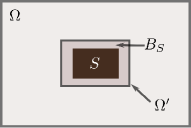
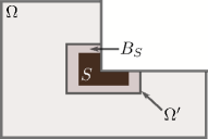
(a) Square domain.    (b) L-shaped domain.   (c) Graph of $\alpha_{(a,b)}(x).$

Figure 2: Definition of the weight function $\alpha$.

To construct a concrete weight function $\alpha(x,y)$, let us define $\alpha_{(a,b)}$ over interval $(a,b)$ as follows.

$$\alpha_{(a,b)}(x):=\left\{\begin{array}[]{ll}1+(x-a)/\varepsilon&x\in(a-\varepsilon,a]\\ 1&x\in(a,b)\\ 1-(x-b)/\varepsilon&x\in[b,b+\varepsilon)\\ 0&\mbox{otherwise}\end{array}\right.\>.$$

Refer to Figure 2-(c) for the graph of $\alpha_{(a,b)}$. For $S$ being a rectangular subdomain constructed by the Cartesian product of two open intervals $(x_{a},x_{b})$, $(y_{a},y_{b})$, the weight function $\alpha$ can be defined by $\alpha(x,y)=\min{\{\alpha_{(x_{a},x_{b})}(x),\alpha_{(y_{a},y_{b})}(y)\}}$.

The weighted inner product and norm are defined by using $\alpha$ as follows.

• Weighted inner product $(\cdot,\cdot)_{\alpha}$:   For $f,g\in L^{2}(\Omega)$ or $f,g\in(L^{2}(\Omega))^{2}$,

  $$(f,g)_{\alpha}:=\int_{\Omega^{\prime}}\alpha f\cdot g~{}dx.$$

• Weighted norm $\|\cdot\|_{\alpha}:~{}$ For $f\in L^{2}(\Omega)$,

  $$\|f\|_{\alpha}:=\sqrt{(f,f)_{\alpha}}=\sqrt{\int_{\Omega^{\prime}}f^{2}\alpha~{}dx}\quad(=\left\|f\sqrt{\alpha}\right\|_{\Omega}).$$

The following inequalities hold.

(14) $$\|f\|_{S}\leq\|f\|_{\alpha}\leq\|f\|_{\Omega^{\prime}}\leq\|f\|_{\Omega}.$$

4.2 Weighted hypercircle formula

In this sub-section, a weighted hypercircle formula is proposed, which can be regarded as an extention to the classical Prager–Synge theorem below.

Theorem 4.1 (Prager–Synge’s theorem[20]).

Let $\phi$ be the solution of (8). For any $v\in V_{0}$ and $\widetilde{\mathbf{p}}\in H(\mbox{\em div};\Omega)$ satisfying

$$\mbox{\em{div} }\widetilde{\mathbf{p}}+f=0,~{}\widetilde{\mathbf{p}}\cdot\mathbf{n}=0\mbox{ on }\Gamma_{N}\>,$$

we have,

(15) $$\|\nabla\phi-\nabla v\|_{\Omega}^{2}+\|\nabla\phi-\widetilde{\mathbf{p}}\|_{\Omega}^{2}=\|\nabla v-\widetilde{\mathbf{p}}\|_{\Omega}^{2}.$$

For weighted norms introduced in the previous section, we have the following extended formulation of the hypercircle (15).

Theorem 4.2.

Let $u$ be the solution of (2). For any $v\in V_{0}$ and $\mathbf{p}\in H(\mbox{\em div};\Omega)$ satisfying

$$\mbox{\em div }\mathbf{p}+f=0\mbox{ in }\Omega,\quad\mathbf{p}\cdot\mathbf{n}=g_{N}\mbox{ on }\Gamma_{N}.$$

Then,

$$\|\nabla u-\nabla v\|_{\alpha}^{2}+\|\nabla u-\mathbf{p}\|_{\alpha}^{2}\leq\|\nabla v-\mathbf{p}\|_{\alpha}^{2}+2\sqrt{2}\|\nabla\alpha\|_{L^{\infty}(\Omega)}\|u-v\|_{\Omega^{\prime}}\|\nabla u-\mathbf{p}\|_{\Omega^{\prime}}.$$

Proof 4.3.

The expansion of $\|\nabla v-\mathbf{p}\|_{\alpha}^{2}=\|(\nabla v-\nabla u)+(\nabla u-\mathbf{p})\|_{\alpha}^{2}$ tells that

(16) $$\|\nabla v-\mathbf{p}\|_{\alpha}^{2}=\|\nabla v-\nabla u\|_{\alpha}^{2}+\|\nabla u-\mathbf{p}\|_{\alpha}^{2}+2(\nabla v-\nabla u,\nabla u-\mathbf{p})_{\alpha}.$$

Let $w:=v-u$. Below, we show the estimation for the cross-term of (16), i.e., $(\nabla w,\nabla u-\mathbf{p})_{\alpha}$.

To deal with $(\nabla w,\nabla u)_{\alpha}$, let us take the test function as $\alpha w$ in (3) and apply the chain rule to $\alpha w$, i.e., $\nabla(\alpha w)=w\nabla\alpha+\alpha\nabla w$. Then we have

(17) $$(\nabla w,\nabla u)_{\alpha}=-\int_{\Omega}w\nabla\alpha\cdot\nabla u~{}dx+\int_{\Omega}f\cdot(\alpha w)~{}dx+\int_{\Gamma_{N}}g_{N}\cdot(\alpha w)ds.$$

For $(\nabla w,\mathbf{p})_{\alpha}$, Green’s formula tells that

(18) $$(\nabla w,\mathbf{p})_{\alpha} = \int_{\Omega}\nabla w\cdot(\alpha\mathbf{p})~{}dx=\int_{\Gamma_{N}}g_{N}\cdot(\alpha w)ds-\int_{\Omega}w\mbox{ div}(\alpha\mathbf{p})~{}dx$$

$$= \int_{\Gamma_{N}}g_{N}\cdot(\alpha w)ds-\int_{\Omega}(\alpha w)\mbox{ div }\mathbf{p}~{}dx-\int_{\Omega}w\nabla\alpha\cdot\mathbf{p}~{}dx.$$

$$= -\int_{\Omega}w\nabla\alpha\cdot\mathbf{p}~{}dx+\int_{\Omega}(\alpha w)f~{}dx+\int_{\Gamma_{N}}g_{N}\cdot(\alpha w)ds.$$

By taking (17)-(18) and noticing that $\alpha=0$ on $\Omega\setminus\Omega^{\prime}$, we have

$$(\nabla v-\nabla u,\nabla u-\mathbf{p})_{\alpha}=-\int_{\Omega}(v-u)\nabla\alpha\cdot(\nabla u-\mathbf{p})~{}dx=-\int_{\Omega^{\prime}}(v-u)\nabla\alpha\cdot(\nabla u-\mathbf{p})~{}dx.$$

By applying Hölder’s inequality, we have

(19) $$|(\nabla v-\nabla u,\nabla u-\mathbf{p})_{\alpha}|\leq\sqrt{2}\|\nabla\alpha\|_{L^{\infty}(\Omega)}\|u-v\|_{\Omega^{\prime}}\|\nabla u-\mathbf{p}\|_{\Omega^{\prime}}.$$

From (16) and (19), we draw the conclusion.

Remark 4.4.

Theorem 4.2 holds no matter $\partial S\cap\partial\Omega=\emptyset$ or not, as can be confirmed in the proof.

4.3 A posteriori local error estimation for finite element solutions

As a preparation to the argument of the main result, let us follow the idea of Kikuchi [11] to introduce auxiliary functions $\overline{u}\in V$ and $\overline{u}_{h}\in V_{h}$ as the solutions to the following equations.

(20) $$(\nabla\overline{u},\nabla v) = (\pi_{h}f,v)+(g_{N},v)_{\Gamma_{N}},~{}\forall v\in V_{0}\>;$$

(21) $$(\nabla\overline{u}_{h},\nabla v_{h}) = (\pi_{h}f,v_{h})+(g_{N},v_{h})_{\Gamma_{N}},~{}\forall v_{h}\in V_{h,0}\>.$$

Both the functions are introduced only for error analysis in a theoretical way, and the above equations do not need to be solved explicitly.

Lemma 4.5.

For $\overline{u}$ of (20) and $\overline{u}_{h}$ of (21), the following estimations hold.

(22) $$|u-\overline{u}|_{H^{1}(\Omega)}\leq C_{0}h\|f-\pi_{h}f\|_{\Omega},$$

(23) $$|u_{h}-\overline{u}_{h}|_{H^{1}(\Omega)}\leq C_{0}h\|f-\pi_{h}f\|_{\Omega}.$$

Here, $C_{0}$ is the projection error constant defined in (7).

Proof 4.6.

According to the definitions of $u$ and $\overline{u}$,

$$(\nabla(u-\overline{u}),\nabla v)=(f-\pi_{h}f,v)=(f-\pi_{h}f,v-\pi_{h}v),\quad v\in V_{0}.$$

By taking $v=u-\overline{u}$ in the above equation and using the error estimation of projection $\pi_{h}$ in (6), we have

$$|u-\overline{u}|_{H^{1}(\Omega)}^{2}=|(\nabla(u-\overline{u}),\nabla(u-\overline{u}))|\leq\|f-\pi_{h}f\|_{\Omega}\cdot C_{0}h|u-\overline{u}|_{H^{1}(\Omega)}.$$

Hence,

$$|u-\overline{u}|_{H^{1}(\Omega)}\leq C_{0}h\|f-\pi_{h}f\|_{\Omega}.$$

Estimation (23) is obtained in the same way.

With the selected $\pi_{h}f\in X_{h}$, the property $\mbox{div}(RT_{h})=X_{h}$ makes it possible to find $\mathbf{p}_{h}\in RT_{h}$ such that

(24) $$\mbox{div }\mathbf{p}_{h}+\pi_{h}f=0,~{}\mathbf{p}_{h}\cdot\mathbf{n}=g_{N}\mbox{ on }\Gamma_{N}\>.$$

In this case, the following hypercircle equation holds:

(25) $$\|\nabla\overline{u}-\nabla v_{h}\|^{2}_{\Omega}+\|\nabla\overline{u}-\mathbf{p}_{h}\|^{2}_{\Omega}=\|\nabla v_{h}-\mathbf{p}_{h}\|^{2}_{\Omega}\>.$$

Remark 4.7.

The estimation (22) along with the hypercircle (25) leads to an a posteriori estimation of the global error.

(26) $$\|\nabla(u-u_{h})\|_{\Omega}\leq\|\nabla u_{h}-\mathbf{p}_{h}\|_{\Omega}+C_{0}h\|f-\pi_{h}f\|_{\Omega}\>.$$

Here, $\mathbf{p}_{h}$ can be chosen freely to approximate $\nabla u$ under the condition (24).

Below, we apply Theorem 4.2 to the current function settings.

Lemma 4.8.

Let $\overline{u}$ and $\overline{u}_{h}$ be the solutions of (20) and (21), respectively. For $\mathbf{p}_{h}\in RT_{h}$ satisfying (24), the following estimation holds,

$$\|\nabla(\overline{u}-\overline{u}_{h})\|_{\alpha}^{2}\leq\|\nabla\overline{u}_{h}-\mathbf{p}_{h}\|_{\alpha}^{2}+2\sqrt{2}\|\nabla\alpha\|_{L^{\infty}(\Omega)}\|\overline{u}-\overline{u}_{h}\|_{\Omega}~{}\|\nabla\overline{u}-\mathbf{p}_{h}\|_{\Omega}.$$

Proof 4.9.

Take $f:=\pi_{h}f,~{}\mathbf{p}:=\mathbf{p}_{h},~{}u:=\overline{u}$ and $v:=\overline{u}_{h}$ in Theorem 4.2, then the following inequality holds.

$$\|\nabla(\overline{u}-\overline{u}_{h})\|_{\alpha}^{2}+\|\nabla\overline{u}-\mathbf{p}_{h}\|_{\alpha}^{2}\leq\|\nabla\overline{u}_{h}-\mathbf{p}_{h}\|_{\alpha}^{2}+2\sqrt{2}\|\nabla\alpha\|_{L^{\infty}(\Omega)}\|\overline{u}-\overline{u}_{h}\|_{\Omega^{\prime}}~{}\|\nabla\overline{u}-\mathbf{p}_{h}\|_{\Omega^{\prime}}.$$

Because $\Omega^{\prime}\subset\Omega$, we conclude by replacing $\|\cdot\|_{\Omega^{\prime}}$ with $\|\cdot\|_{\Omega}$.

To state the results in Theorem 4.10 and 4.12, let us define the following four computable quantities $\overline{E}_{1},~{}\overline{E}_{2},~{}E_{1}$ and $E_{2}$.

$$\overline{E}_{1}:=\|\nabla\overline{u}_{h}-\mathbf{p}_{h}\|_{\alpha},\quad E_{1}:=\|\nabla u_{h}-\mathbf{p}_{h}\|_{\alpha}+C_{0}h\|f-\pi_{h}f\|_{\Omega},$$

$$\overline{E}_{2}:=\left\{2\sqrt{2}C(h)\cdot\|\nabla\alpha\|_{L^{\infty}(\Omega)}\right\}^{1/2}\cdot\|\nabla\overline{u}_{h}-\mathbf{p}_{h}\|_{\Omega},$$

$$E_{2}:=\left\{2\sqrt{2}C(h)\cdot\|\nabla\alpha\|_{L^{\infty}(\Omega)}\right\}^{1/2}\cdot\|\nabla u_{h}-\mathbf{p}_{h}\|_{\Omega}\>.~{}$$

Theorem 4.10 (A posteriori local error estimation for $\overline{u}$).

Let $u$ and $\overline{u}_{h}$ be the solutions of (3), (21), respectively. For $\mathbf{p}_{h}\in RT_{h}$ satisfying

$$\mbox{\em{div} }\mathbf{p}_{h}+\pi_{h}f=0,~{}\mathbf{p}_{h}\cdot\mathbf{n}=g_{N}\mbox{ on }\Gamma_{N}~{},$$

the following local error estimation holds.

(27) $$\|\nabla u-\nabla\overline{u}_{h}\|_{S}\leq\sqrt{\overline{E}_{1}^{2}+\overline{E}_{2}^{2}}+C_{0}h\|f-\pi_{h}f\|_{\Omega}.$$

Proof 4.11.

With $\overline{u}$ defined in (20) and the triangle inequality, we obtain:

$$\|\nabla(u-\overline{u}_{h})\|_{S}\leq\|\nabla(u-\overline{u})\|_{S}+\|\nabla(\overline{u}-\overline{u}_{h})\|_{S}\leq\|\nabla(u-\overline{u})\|_{\Omega}+\|\nabla(\overline{u}-\overline{u}_{h})\|_{\alpha}.$$

By applying the estimation of $\|\nabla(u-\overline{u})\|_{\Omega}$ in Lemma 4.5 and the estimation of $\|\nabla(\overline{u}-\overline{u}_{h})\|_{\alpha}$ in Lemma 4.8, the following estimation holds.

(28) $$\|\nabla(u-\overline{u}_{h})\|_{S} \leq \left\{\|\nabla\overline{u}_{h}-\mathbf{p}_{h}\|_{\alpha}^{2}+2\sqrt{2}\|\nabla\alpha\|_{\infty}\|\overline{u}-\overline{u}_{h}\|_{\Omega}~{}\|\nabla\overline{u}-\mathbf{p}_{h}\|_{\Omega}\right\}^{\frac{1}{2}}$$

$$+C_{0}h\|f-\pi_{h}f\|_{\Omega}\>.$$

Next, we give the estimation for $\|\overline{u}-\overline{u}_{h}\|_{\Omega},~{}\|\nabla\overline{u}-\mathbf{p}_{h}\|_{\Omega}$ in (28).

(a) From Theorem 4.1, the hypercircle below is available for $\overline{u}$ defined in (20),

(29) $$\|\nabla\overline{u}-\nabla v_{h}\|_{\Omega}^{2}+\|\nabla\overline{u}-\mathbf{p}_{h}\|_{\Omega}^{2}=\|\nabla v_{h}-\mathbf{p}_{h}\|_{\Omega}^{2},\quad\forall v_{h}\in V_{h}\>.$$

By taking $v_{h}:=\overline{u}_{h}$, we obtain the estimation of $\|\nabla\overline{u}-\mathbf{p}_{h}\|_{\Omega}$:

(30) $$\|\nabla\overline{u}-\mathbf{p}_{h}\|_{\Omega}\leq\|\nabla\overline{u}_{h}-\mathbf{p}_{h}\|_{\Omega}\>.$$

(b) To give the estimation of $\|\overline{u}-\overline{u}_{h}\|_{\Omega}$, let us define the dual problem.

$$\mbox{Find }\phi\in V_{0}\mbox{ s.t. }(\nabla\phi,\nabla v)=(\overline{u}-\overline{u}_{h},v),\quad\forall v\in V_{0}.$$

By applying $P_{h}$ defined in (10) along with the a priori estimation (11) in Theorem 3.1, we have,

$$\|\overline{u}-\overline{u}_{h}\|_{\Omega}^{2} \leq \|\nabla(\phi-P_{h}\phi)\|_{\Omega}\cdot\|\nabla(\overline{u}-\overline{u}_{h})\|_{\Omega}.$$

$$\leq C(h)\>\|\overline{u}-\overline{u}_{h}\|_{\Omega}\cdot\|\nabla(\overline{u}-\overline{u}_{h})\|_{\Omega}.$$

Notice that (29) with $v_{h}:=\overline{u}_{h}$ implies

$$\|\nabla\overline{u}-\nabla\overline{u}_{h}\|_{\Omega}\leq\|\nabla\overline{u}_{h}-\mathbf{p}_{h}\|_{\Omega}\>.$$

Thus, we have the estimation of $\|\overline{u}-\overline{u}_{h}\|_{\Omega}$:

(31) $$\|\overline{u}-\overline{u}_{h}\|_{\Omega}\leq C(h)\|\nabla(\overline{u}-\overline{u}_{h})\|_{\Omega}\leq C(h)\|\nabla\overline{u}_{h}-\mathbf{p}_{h}\|_{\Omega}.$$

Apply (30) and (31) to the first term of the right-hand side of (28),

$$\|\nabla\overline{u}_{h}-\mathbf{p}_{h}\|_{\alpha}^{2}+2\sqrt{2}\>\|\nabla\alpha\|_{\infty}\|\overline{u}-\overline{u}_{h}\|_{\Omega}~{}\|\nabla\overline{u}-\mathbf{p}_{h}\|_{\Omega}$$

$$\leq\|\nabla\overline{u}_{h}-\mathbf{p}_{h}\|_{\alpha}^{2}+2\sqrt{2}\>\|\nabla\alpha\|_{\infty}\>C(h)\>\|\nabla\overline{u}_{h}-\mathbf{p}_{h}\|_{\Omega}^{2}$$

$$={\overline{E}_{1}^{2}+\overline{E}_{2}^{2}}.$$

Now, we draw the conclusion by sorting the estimation of (28).

Theorem 4.12.

Under the assumptions of Theorem 4.10, the following estimation holds.

(32) $$\|\nabla u-\nabla u_{h}\|_{S}\leq\sqrt{E_{1}^{2}+E_{2}^{2}}+2C_{0}h\|f-\pi_{h}f\|_{\Omega}\>.$$

Proof 4.13.

First, we apply the triangle inequality to $(u-\overline{u}_{h})+(\overline{u}_{h}-{u}_{h})$ and the estimation (23) in Lemma 4.5 to have,

$$\|\nabla(u-{u}_{h})\|_{S}\leq\|\nabla(u_{h}-\overline{u}_{h})\|_{S}+\|\nabla(u-\overline{u}_{h})\|_{S}\leq C_{0}h\|f-\pi_{h}f\|_{\Omega}+\|\nabla({u}-\overline{u}_{h})\|_{S}\>.$$

Next, we apply the result in Theorem 4.10 to $\|\nabla({u}-\overline{u}_{h})\|_{S}$ and process the term $\overline{u}_{h}$ in $\overline{E}_{1}$ and $\overline{E}_{2}$. Because $\overline{u}_{h}$ is the best approximation to $\overline{u}$ in $V_{h}$, the hypercircle (25) with respect to $\pi_{h}f$ leads to

$$\|\nabla\overline{u}_{h}-\mathbf{p}_{h}\|_{\Omega}\leq\|\nabla u_{h}-\mathbf{p}_{h}\|_{\Omega}\>.$$

For the term $\|\nabla\overline{u}_{h}-\mathbf{p}_{h}\|_{\alpha}$ in $\overline{E}_{2}$ , apply the triangle inequality and (23) to obtain

$$\|\nabla\overline{u}_{h}-\mathbf{p}_{h}\|_{\alpha}\leq\|\nabla(\overline{u}_{h}-u_{h})\|_{\alpha}+\|\nabla u_{h}-\mathbf{p}_{h}\|_{\alpha}\leq C_{0}h\|f-\pi_{h}f\|_{\Omega}+\|\nabla u_{h}-\mathbf{p}_{h}\|_{\alpha}\>.$$

Now, we can conclude as in (32).

5 Convergence analysis and application to non-uniform mesh

In this section, we have an analysis on the convergence behavior for the proposed a posteriori error estimation and show its application in efficient computing with non-uniform meshes.

For a solution $u\in H^{2}$ solved by FEM over a uniform mesh with mesh size $h$, the global error terms $\|\nabla u_{h}-\mathbf{p}_{h}\|_{\Omega}$ and $C(h)$ have the convergence rate as $O(h)$. Thus, the following convergence rate is available in Theorem 4.12 .

(33) $$E_{1}=O(h),~{}E_{2}=O(h^{1.5});~{}~{}\|\nabla u-\nabla u_{h}\|_{S}\leq O(h)$$

Note that the order of $E_{2}$ can be further improved by selecting the Raviart-Thomas FEM space with higher degree and theoretically $E_{2}$ can be arbitrarily small by selecting a good approximation of $\mathbf{p}_{h}$ to $\overline{u}$ using an independent quite refined mesh. Below is a detailed argument for this property.

Improving convergence rate of the global error term. Let $V_{h}^{k},~{}RT_{h}^{k-1}$ $(k\geq 1)$ be the conforming finite element space of degree $k$ and the Raviart-Thomas FEM space of degree $k-1$, respectively. Suppose $\overline{u}$ defined in (20) has $H^{2}$-regularity. Let us consider the following FEM solutions corresponding to $\overline{u}$:

• $\overline{w}_{h}\in V_{h}^{k}$ as the best approximation to $\overline{u}$ under $|\cdot|_{1}$ norm ;

• $\widetilde{\mathbf{p}}_{h}\in RT_{h}^{k-1}$ as the best approximation to $\nabla\overline{u}$ under $L^{2}$ norm, subject to the condition (24).

Then the following hypercircle equation holds.

$$\|\nabla\overline{u}-\nabla\overline{w}_{h}\|_{\Omega}^{2}+\|\nabla\overline{u}-\widetilde{\mathbf{p}}_{h}\|_{\Omega}^{2}=\|\nabla\overline{w}_{h}-\widetilde{\mathbf{p}}_{h}\|_{\Omega}^{2}\>.$$

Since for a smooth enough solution $\overline{u}$, both $\|\nabla\overline{u}-\nabla\overline{w}_{h}\|_{\Omega}$ and $\|\nabla\overline{u}-\widetilde{\mathbf{p}}_{h}\|_{\Omega}$ have the convergence rate as $O(h^{k})$, we have

$$(\|\nabla\overline{u}-\widetilde{\mathbf{p}}_{h}\|_{\Omega}\leq)\|\nabla\overline{w}_{h}-\widetilde{\mathbf{p}}_{h}\|_{\Omega}=O(h^{k})~{}~{}(k\geq 2)\>.$$

By replacing the estimation of (30) with $\|\nabla\overline{u}-\widetilde{\mathbf{p}}_{h}\|_{\Omega}\leq\|\nabla\overline{w}_{h}-\widetilde{\mathbf{p}}_{h}\|_{\Omega}$, the global error terms $E_{2},\overline{E}_{2}$ in Theorem 4.10 and 4.12 become

$$\overline{E}_{2}:=\left\{2\sqrt{2}C(h)\cdot\|\nabla\alpha\|_{L^{\infty}(\Omega)}\cdot\|\nabla\overline{u}_{h}-\widetilde{\mathbf{p}}_{h}\|_{\Omega}\cdot\|\nabla\overline{w}_{h}-\widetilde{\mathbf{p}}_{h}\|_{\Omega}\>\right\}^{1/2},~{}$$

$$E_{2}:=\left\{2\sqrt{2}C(h)\cdot\|\nabla\alpha\|_{L^{\infty}(\Omega)}\cdot\|\nabla u_{h}-\widetilde{\mathbf{p}}_{h}\|_{\Omega}\cdot\|\nabla\overline{w}_{h}-\widetilde{\mathbf{p}}_{h}\|_{\Omega}\>\right\}^{1/2}.~{}$$

Note that both $\|\nabla\overline{u}_{h}-\widetilde{\mathbf{p}}_{h}\|_{\Omega}$ and $\|\nabla u_{h}-\widetilde{\mathbf{p}}_{h}\|_{\Omega}$ have the convergence rate as $O(h)$, which can be confirmed by utilizing the hypercircle involving $\overline{u},\overline{u}_{h}$ and $\mathbf{p}_{h}$. Therefore we have the convergence rate as

(34) $$E_{2},\overline{E}_{2}=O(h^{(1+k/2)})\>(k\geq 1).$$

It is worth to point out the selection of $\overline{w}_{h}$ and $\mathbf{p}_{h}$ is independent on the objective FEM solution $u_{h}$. Thus, a large value of $k(\geq 2)$ will result in an improved convergence rate for global error terms; see numerical results in Figure 8, 10 of §6.2. Application to non-uniform mesh. Theoretical analysis on local error estimation tells that for $u\in H^{2}(\Omega)$ ([25, 26]):

(35) $$\|u-u_{h}\|_{1,S}=O(h_{\Omega^{\prime}}+h_{G}^{2}).$$

Here, $h_{\Omega^{\prime}}$ denotes the mesh size of $\Omega^{\prime}$; $h_{G}$ the one for the mesh outside of $\Omega^{\prime}$. Estimation (35) implies an asymptotically optimal error with rate $O(h_{\Omega^{\prime}})$ in $H^{1}$ norm locally by taking $h_{G}=O(\sqrt{h_{\Omega^{\prime}}})$.

Such a priori estimation motivates us to apply our proposed a posteriori error estimator to non-uniform meshes to have more efficient computation and error estimation. Here, the local error estimator in Theorem 4.12 is denoted by

$$\widehat{E}_{L}:=\sqrt{E_{1}^{2}+E_{2}^{2}}+2C_{0}h_{G}\|f-\pi_{h}f\|_{\Omega}\>.$$

For $f\in H^{1}(\Omega)$, the convergence rate of the projection error term $C_{0}h\|f-\pi_{h}f\|$ in $E_{1}$ is $O(h_{G}^{2})$. For the error term $E_{1}$, it is expected that the local term $\|\nabla u_{h}-\mathbf{p}_{h}\|_{\alpha}=O(h_{\Omega^{\prime}}+h_{G}^{2})$. However, such a result is not discussed yet in the existing literature. In this paper, rather than theoretical analysis, by numerical experiment in §6.2, we confirm the asymptotic behavior of $E_{1}=O(h_{\Omega^{\prime}})$ over a non-uniform mesh when the mesh size is selected as $h_{G}=\sqrt{h_{\Omega^{\prime}}}$. With analogous argument to the one for (34), it is easy to see that the convergence rate of the global error term $E_{2}$ and $\overline{E}_{2}$ are dominated by the global mesh size $h_{G}$:

(36) $$E_{2},\overline{E}_{2}=O(h_{G}^{(1+k/2)})\>(k\geq 1).$$

In §6.2, by numerical examples, we investigate the the convergence rate of error estimators when the mesh size is chosen as $h_{G}=\sqrt{h_{\Omega^{\prime}}}$. In case that only $u_{h}\in V_{h}^{(1)}$ and $\mathbf{p}_{h}\in RT_{h}^{(0)}$ are used in the local error estimation, it is validated that

$$E_{1}=O(h_{\Omega^{\prime}}),~{}E_{2}=O(h_{G}^{1.5});~{}~{}\widehat{E}_{L}\leq O(h_{\Omega^{\prime}}+h_{G}^{1.5}).$$

In case that $\overline{w}_{h}\in V_{h}^{(k)}$ and $\widetilde{\mathbf{p}}_{h}\in RT_{h}^{(k-1)}~{}(k\geq 2)$ along with (36) are also used in the local error estimation, we have

$$E_{1}=O(h_{\Omega^{\prime}}),~{}E_{2}=O(h_{G}^{(1+k/2)});~{}~{}\widehat{E}_{L}\leq O(h_{\Omega^{\prime}}+h_{G}^{(1+k/2)}).$$

6 Numerical experiments

6.1 Preparation

The selection of bandwidth of the $B_{S}$ is important in the local error estimation. A large bandwidth of $B_{S}$ leads to a large value of $E_{1}$, while a small bandwidth of $B_{S}$ results in a large value of $\|\nabla\alpha\|_{L^{\infty}(\Omega)}$ in $E_{2}$. Therefore, in each example, we first investigate the impact of the bandwidth of $B_{S}$, and then take an appropriate width of $B_{S}$ for subsequent computation.

Besides the symbols $E_{1},E_{2}$ in (32), we introduce new symbols as follows:

• The local error is denoted by

  $$E_{L}:=\|\nabla u-\nabla u_{h}\|_{S}.\quad\widehat{E}_{L}:=\sqrt{E_{1}^{2}+E_{2}^{2}}+2C_{0}h\|f-\pi_{h}f\|_{\Omega}\>.$$

• The global error and its estimation in (26) are denoted by

  $$E_{G}:=\|\nabla u-\nabla u_{h}\|_{\Omega},\quad\widehat{E}_{G}:=\|\nabla u_{h}-\mathbf{p}_{h}\|_{\Omega}+C_{0}h\|f-\pi_{h}f\|_{\Omega}.$$

Here, $u_{h}\in V_{h}$ and $\mathbf{p}_{h}\in RT_{h}$ are finite element solutions of the objective problems; $\mathbf{p}_{h}$ also satisfies the condition (24).

6.2 Square domain

The error estimation proposed in this paper is applicable to problems with different boundary conditions. To illustrate this feature, let us consider the following Poisson equations over the unit square domain $\Omega=(0,1)^{2}$, where the subdomain is selected as $S=(0.375,0.625)^{2}$.

1. Dirichlet boundary condition (exact solution $u=\sin(\pi x)\sin(\pi y)$).

   (37) $$-\Delta u=2\pi^{2}\sin(\pi x)\sin(\pi y)\mbox{ in }\Omega,\quad u=0\mbox{ on }\partial\Omega.$$

2. Neumann boundary condition (exact solution $u=\cos(\pi x)\cos(\pi y)$).

   (38) $$-\Delta u=2\pi^{2}\cos(\pi x)\cos(\pi y)\mbox{ in }\Omega,\quad\frac{\partial u}{\partial\mathbf{n}}=0\mbox{ on }\partial\Omega,\quad\int_{\Omega}udx=0\>.$$

The finite element solutions $u_{h},\mathbf{p}_{h}$ are computed with uniform meshes, and the mesh size $h$ here is chosen as the leg length of the triangle element for an uniform mesh.

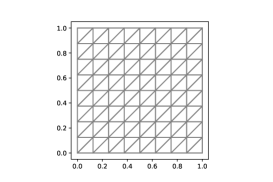
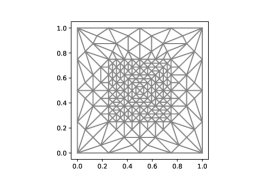
Figure 3: Uniform and non-uniform mesh (Rectangle domain).

Figure 4: Dependency of local error estimation on the bandwidth of $B_{S}$ (Dirichlet BVP and square domain, uniform mesh).

Figure 5: Dependency of local error estimation on the bandwidth of $B_{S}$ (Neumann BVP and square domain, uniform mesh).

Asymptotic behavior of the proposed local error estimator over a uniform mesh. For Dirichlet and Neumann boundary conditions, the dependencies of the local error estimator $\widehat{E}_{L}$ on the bandwidth of $B_{S}$ are shown in Figure 5 and Figure 5, respectively. The relative variation of local error estimator with respect to bandwidth selection is displayed for two problems. It is noteworthy that the local error estimation is not significantly sensitive to variations in bandwidth. For example, in Figure 5, for $h=1/64$, the relative variation in error estimation with respect to a bandwidth in the range $[0.125,0.275]$ is less than 5%.

In the following discussion, the bandwidth of $B_{S}$ is selected as $0.15$ for the Dirichlet boundary condition and $0.10$ for the Neumann boundary condition.

Figure 6: Error estimators for Dirichlet BVP (square domain, uniform mesh).

Figure 7: Error estimators for Neumann BVP (square domain, uniform mesh).

Table 1: Error estimate for Dirichlet BVP (square domain , uniform mesh)

$h$	$\kappa_{h}$	$C(h)$	$E_{L}$	$E_{1}$	$E_{2}$	$\widehat{E}_{L}$	$\widehat{E}_{G}$
1/16	0.030	0.036	0.060	0.106	0.206	0.258	0.264
1/32	0.015	0.018	0.030	0.049	0.074	0.095	0.129
1/64	0.008	0.009	0.015	0.024	0.026	0.037	0.064
1/128	0.004	0.005	0.007	0.012	0.009	0.015	0.032
1/256	0.002	0.002	0.004	0.006	0.003	0.007	0.016

Table 2: Error estimate for Neumann BVP (square domain, uniform mesh).

$h$	$\kappa_{h}$	$C(h)$	$E_{L}$	$E_{1}$	$E_{2}$	$\widehat{E}_{L}$	$\widehat{E}_{G}$
1/16	0.030	0.036	0.084	0.153	0.252	0.320	0.263
1/32	0.015	0.018	0.042	0.073	0.090	0.122	0.129
1/64	0.008	0.009	0.021	0.036	0.032	0.049	0.064
1/128	0.004	0.005	0.011	0.018	0.011	0.021	0.032
1/256	0.002	0.002	0.005	0.010	0.004	0.010	0.016

A detailed discussion on each component of the error estimators is also presented; see Table 1 and Figure 7 for Dirichlet boundary condition, Table 2 and Figure 7 for Neumann boundary condition. From the numerical results, we confirm that for both the problems the main term $E_{1}$ of the error estimation (32) becomes dominant when $h\leq 1/128$, which agrees with the analysis in §5.

Improved convergence rate of the global error term $E_{2}$. Here, we confirm the improvement of the local error estimator discussed in §5, when the approximation $\mathbf{p}_{h}$ to $\nabla u$ is obtained in a higher degree Raviart-Thomas FEM space. Table 3 and Figure 8 show that the global error term $E_{2}$ has an improved convergence rate as $O(h^{2})$ by using $\mathbf{p}_{h}\in RT_{h}^{1}$. The numerical results support the theoretical result (34).

Figure 8: Improved convergence rate of the local error estimator (34) with $\overline{w}_{h}\in V_{h}^{2}$, $\mathbf{p}_{h}\in RT_{h}^{1}$ (uniform mesh for squared domain).

Table 3: Convergence rate of $E_{2}$ w.r.t. the selection of $\mathbf{p_{h}}\in RT_{h}^{k-1}$.

$h$	$E_{2}$ $(k=1)$	Order	$E_{2}(k=2)$	Order
1/16	0.206	-	0.036	-
1/32	0.074	1.484	0.009	1.982
1/64	0.026	1.493	0.002	1.992
1/128	0.009	1.497	5.7e-4	1.997
1/256	0.003	1.499	1.4e-4	1.999

Convergence behavior for non-uniform meshes. Based on numerical results, we investigate the behavior of our proposed estimator (32) for non-uniform meshes under the setting $h_{G}=O(\sqrt{h_{\Omega^{\prime}}})$; see a sample non-uniform mesh in Figure 3. The subdomain $S$ and the bandwidth $B_{S}$ are set to $(0.375,0.625)^{2}$ and $0.125$, respectively.

Figure 9: Local error estimator for lowest order FEM over non-uniform mesh (squared domain).

Figure 10: Improvement of the local error estimator (32) for FEM of higher degree over non-uniform meshes (squared domain).

Table 4: Convergence rate of $\|\nabla u_{h}-\mathbf{p}_{h}\|_{\alpha}$ over non-uniform mesh (squared domain).

$h_{\Omega^{\prime}}$	$\|\nabla u_{h}-\mathbf{p}_{h}\|_{\alpha}$	Order
0.177	0.221	-
0.044	0.059	0.957
0.011	0.015	1.007
0.003	0.004	0.997

The numerical results in Figure 9 and Table 4 show that the convergence rates of $\|\nabla u_{h}-\mathbf{p}_{h}\|_{\alpha}$ and $E_{1}$ are almost $O(h_{\Omega^{\prime}})$. The numerical results support the expectation that $\|\nabla u_{h}-\mathbf{p}_{h}\|_{\alpha}=O(h_{\Omega^{\prime}})$ under current mesh configuration (i.e., $h_{G}=\sqrt{h_{\Omega^{\prime}}}$). In case that the lowest degree Raviart-Thomas FEM employed to compute the global term $E_{2}$, the convergence rate of the estimator $\widehat{E}_{L}$ is approximately $O(h_{\Omega^{\prime}}^{0.75})$. When $\tilde{p}_{h}$ is selected from $RT^{(1)}$, the convergence rate of $E_{2}$ and $\widehat{E}_{L}$ is improved to be $O(h_{\Omega^{\prime}})$; see Figure 10. The theoretical convergence rate of $\|\nabla u_{h}-\mathbf{p}_{h}\|_{\alpha}$ will be considered in our succeeding research.

As a conclusion, our proposed local error estimator is dominated by the local error term $E_{1}=O(h_{\Omega^{\prime}})$. Thus, it is possible to increase the efficiency of computation by using a non-uniform mesh with a raw triangulation for the subdomain outside of the part of interest.

6.3 L-shaped domain

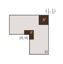
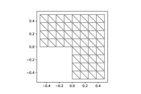
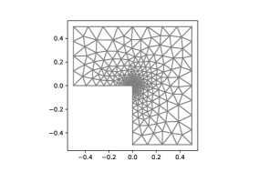
Figure 11: Uniform and non-uniform mesh for an L-shaped domain $\Omega$ with two subdomains $S$, $S^{\prime}$.

The proposed error estimation (32) is applicable to problems with a singular solution and the even case in which the subdomain $S$ and $\Omega$ share a common part of the boundary. In this sub-section, we consider the boundary value problem over an L-shaped domain $\Omega:=(-0.5,0.5)^{2}\setminus[-0.5,0]^{2}$; see Figure 11. The error estimation on two subdomains $S=\Omega\cap(-0.125,0.125)^{2}$ and $S^{\prime}=(0.25,~{}0.5)^{2}$ will be considered.

Let $u=r^{\frac{2}{3}}\sin{\left(\frac{2}{3}(\theta+\frac{\pi}{2})\right)}\cos{(\pi x)}\cos{(\pi y)}$, where $r$ and $\theta$ are the variables under the polar coordinates. Define $f=-\Delta u$. Then $u$ is the solution of the following equation.

(39) $$-\Delta u=f\mbox{ in }\Omega,\quad u=0\mbox{ on }\partial\Omega.$$

It is easy to confirm that $u\notin H^{2}(\Omega)$ due to the singularity around the re-entry corner point of the domain.

Selection of the bandwidth of $B_{S}$. The dependency of $\widehat{E}_{L}$ on the bandwidth of the $B_{S}$ is shown in Figure 12. In the following computation, the bandwidth of $B_{S},B_{S^{\prime}}$ is selected as $0.375$, $0.25$, respectively.

Figure 12: Dependency of local error estimation on the bandwidth of $B_{S}$ (L-shaped domain).

For subdomain $S$, the asymptotic behavior of $\widehat{E}_{L}$ with respect to mesh size $h$ is shown in the Table 5 and Figure 13. The numerical results tell that the local error component $E_{1}$ in $\widehat{E}_{L}$ gradually becomes dominant as the mesh is refined.

Table 5: Error estimators for subdomain $S$ (uniform mesh of L-shaped domain).

$h$	$\kappa_{h}$	$C(h)$	$E_{L}$	$E_{1}$	$E_{2}$	$\widehat{E}_{L}$	$\widehat{E}_{G}$
1/16	0.046	0.050	0.080	0.139	0.108	0.192	0.172
1/32	0.028	0.029	0.050	0.081	0.047	0.098	0.095
1/64	0.017	0.018	0.032	0.049	0.021	0.054	0.055
1/128	0.011	0.011	0.020	0.030	0.030	0.032	0.032
1/256	0.007	0.006	0.013	0.018	0.005	0.019	0.020

Figure 13: Error estimators for subdomain $S$ (uniform mesh of L-shaped domain).

We also compare $E_{L}$, $\widehat{E}_{L}$ with $E_{G}$, $\widehat{E}_{G}$ in Table 6. Denote $\beta:=E_{L}/E_{G}$ and $\hat{\beta}:=\widehat{E}_{L}$/$\widehat{E}_{G}$. It is observed that the approximation error concentrates in the subdomain $S$ around the re-entry corner as the mesh is refined. For $h=1/256$, the local error in $S$ is about $91\%$ of the global error in the whole domain.

Table 6: Comparison of the estimated local error on $S$ and $S^{\prime}$.

	subdomain $S$		subdomain $S^{\prime}$
$h$	$\beta$(%)	$\hat{\beta}$(%)	$E_{L}$	$\widehat{E}_{L}$	$\beta$(%)	$\hat{\beta}$(%)
1/16	64	112	0.041	0.160	33	93
1/32	73	103	0.021	0.069	30	72
1/64	80	100	0.010	0.031	26	57
1/128	86	99	0.005	0.014	22	45
1/256	91	99	0.003	0.007	18	35

Finally, we consider the local error estimation for a non-uniform mesh; see computation results Table 7 and Figure 14. It is observed that for the subdomain $S$, both $\beta$ and $\hat{\beta}$ become smaller compared to the results in the case of uniform meshes, which implies that a denser mesh around the re-entry corner improves the quality of local approximation.

Table 7: Error estimators for subdomain $S$ (non-uniform mesh of L-shaped domain)

$h$	$\kappa_{h}$	$C(h)$	$E_{L}$	$E_{1}$	$E_{2}$	$\widehat{E}_{L}$	$\widehat{E}_{G}$	$\beta$(%)	$\hat{\beta}$(%)
0.141	0.039	0.054	0.023	0.083	0.106	0.168	0.166	21	101
0.081	0.021	0.030	0.012	0.039	0.040	0.067	0.081	21	82
0.041	0.011	0.015	0.007	0.019	0.015	0.027	0.040	23	67
0.020	0.006	0.008	0.004	0.010	0.005	0.012	0.020	46	60
0.010	0.003	0.004	0.002	0.005	0.002	0.006	0.010	30	57

Figure 14: Error estimators for subdomain $S$ (non-uniform mesh of L-shaped domain).

7 Conclusion and future work

In this study, we proposed an explicit local a posterior error estimation for the finite element solutions and performed numerical experiments on the boundary value problem of the Poisson equation, defined on the square and L-shaped domains. The numerical results show that the proposed method provides an efficient estimation of the local error, especially compared to the general overestimated global error estimation.

In future, we will further apply the local error estimation to the four-probe method used in resistivity measurement. Another promising approach for the explicit point-wise error estimation needed by the four-probe method is to apply the idea of [6] and the hypercircle method to the finite element method.

References

- [1] D. Braess, Finite Elements. Theory, Fast Solvers and Applications in Solid Mechanics, Cambridge University Press, 2007, https://doi.org/10.1017/CBO9780511618635.
- [2] A. Demlow, Local a posteriori estimates for pointwise gradient errors in finite element methods for elliptic problems, Math. Comp., 76 (2007), pp. 19–42, https://doi.org/10.1090/S0025-5718-06-01879-5.
- [3] A. Demlow, Convergence of an adaptive finite element method for controlling local energy error, SIAM J. Numer. Anal., 48 (2010), pp. 470–497.
- [4] A. Demlow, Quasi-optimality of adaptive finite element methods for controlling local energy errors, Numer. Math., 134 (2016), pp. 27–60.
- [5] A. Demlow, J. Guzman, and H. A. Schatz, Local energy estimates for the finite element method on sharply varying grids, Math. Comp., 80 (2011), pp. 1–9, https://doi.org/10.1090/S0025-5718-2010-02353-1.
- [6] H. Fujita, Contribution to the theory of upper and lower bounds in boundary value problems, J. Phys. Soc. Japan, 10 (1955), pp. 1–8, https://doi.org/10.1143/JPSJ.10.1.
- [7] F. E. I. Miccoli, H. Pfnür, and C. Tegenkamp, The 100th anniversary of the four-point probe technique: the role of probe geometries in isotropic and anisotropic systems, J. Phys. Condens. Matter, 27 (2015), p. 223201, https://doi.org/10.1088/0953-8984/27/22/223201, https://doi.org/10.1088/0953-8984/27/22/223201.
- [8] T. Kato, On some approximate methods concerning the operators , Mathematische Annalen, 126 (1953), pp. 253–262.
- [9] F. Kikuchi and X. Liu, Determination of the Babuška-Aziz constant for the linear triangular finite element, Jpn. J. Ind. Appl. Math., 23 (2006), pp. 75–82.
- [10] F. Kikuchi and X. Liu, Estimation of interpolation error constants for the and triangular finite elements, Comput. Methods. Appl. Mech. Eng., 196 (2007), pp. 3750–3758, https://doi.org/https://doi.org/10.1016/j.cma.2006.10.029, https://www.sciencedirect.com/science/article/pii/S0045782507001028.
- [11] F. Kikuchi and H. Saito, Remarks on a posteriori error estimation for finite element solutions, J. Comput. Appl. Mech., 199 (2007), pp. 329–336, https://doi.org/https://doi.org/10.1016/j.cam.2005.07.031, https://www.sciencedirect.com/science/article/pii/S0377042705007685.
- [12] R. S. Laugesen and B. A. Siudeja, Minimizing neumann fundamental tones of triangles: An optimal poincaré inequality, J. Differ. Equ., 249 (2010), pp. 118–135, https://doi.org/https://doi.org/10.1016/j.jde.2010.02.020, https://www.sciencedirect.com/science/article/pii/S0022039610000823.
- [13] Q. Li and X. Liu, Explicit finite element error estimates for nonhomogeneous neumann problems, Appl. Math., 63 (2018), pp. 1–13, https://doi.org/10.21136/AM.2018.0095-18.
- [14] X. Liao and R. Notchetto, Local a posteriori error estimates and adaptive control of pollution effects, Numer. Methods Partial Differential Equations, 19 (2003), pp. 421–442.
- [15] X. Liu and S. Oishi, Verified eigenvalue evaluation for the laplacian over polygonal domains of arbitrary shape, SIAM J. Numer. Anal., 51 (2013), pp. 1634–1654, https://doi.org/10.1137/120878446.
- [16] T. Nakano and X. Liu, Explicit a posteriori local error estimation for finite element solutions, Transactions of the Japan Society for Industrial and Applied Mathematics, 29 (2019), pp. 362–382. (in Japanese).
- [17] P. Neittaanmäki and S. Repin, Reliable methods for computer simulation: error control and a posteriori estimates, Elsevier. Amsterdam, 2004.
- [18] J. A. Nitsche and A. H. Schatz, Interior estimates for ritz-galerkin methods, Math Comput, 28 (1974), pp. 937–958, http://www.jstor.org/stable/2005356.
- [19] S. Oishi, T. Ogita, M. Kashiwagi, X. Liu, et al., Principle of Verified Numerical Computations, CORONA publisher, 2018. (in Japanese).
- [20] W. Prager and J. L. Synge, Approximations in elasticity based on the concept of function space, Q. Appl. Math., 5 (1947), pp. 241–269, http://www.jstor.org/stable/43633616.
- [21] A. H. Schatz, Pointwise error estimates and asymptotic error expansion inequalities for the finite element method on irregular grids: Part i. global estimates, Math. Comp., 67 (1998), pp. 877–899, http://www.jstor.org/stable/2585162.
- [22] A. H. Schatz and L. B. Wahlbin, Interior maximum-norm estimates for finite element methods, part ii, Mathematics of Computation, 64 (1995), pp. 907–928, http://www.jstor.org/stable/2153476.
- [23] L. B. Wahlbin, Local behavior in finite element methods, vol. 2 of Handbook of Numerical Analysis, Elsevier, 1991, pp. 353–522, https://doi.org/https://doi.org/10.1016/S1570-8659(05)80040-7, https://www.sciencedirect.com/science/article/pii/S1570865905800407.
- [24] L. B. Wahlbin, Superconvergence in Galerkin Finite Element Methods, Series Abbreviated Title Lecture Notes in Mathematics, Springer, Berlin, Heidelberg, 1995, https://doi.org/https://doi.org/10.1007/BFb0096835.
- [25] J. Xu and A. Zhou, Local and parallel finite element algorithms based on two-grid discretizations, Math. Comp., 69 (2000), pp. 881–909.
- [26] J. Xu and A. Zhou, Local and parallel finite element algorithms based on two-grid discretizations for nonlinear problems, Adv. Comput. Math., 14 (2001), pp. 293–327.
- [27] M. Yamashita and M. Agu, Geometrical correction factor for semiconductor resistivity measurements by four-point probe method, Jpn. J. Appl. Phys., 23 (1984), pp. 1499–1504, https://doi.org/10.1143/jjap.23.1499, https://doi.org/10.1143/jjap.23.1499.