Kernel Knockoffs Selection for

Nonparametric Additive Models

Xiaowu Dai, Xiang Lyu, and Lexin Li
University of California, Berkeley
To appear in Journal of the American Statistical Association: Theory and Method

11footnotetext: Address for correspondence: Lexin Li, Department of Biostatistics and Epidemiology, University of California, Berkeley, 2121 Berkeley Way, Berkeley, CA 94720, USA. E-mail: lexinli@berkeley.edu. The first two authors contribute equally to the paper.
Abstract

Thanks to its fine balance between model flexibility and interpretability, the nonparametric additive model has been widely used, and variable selection for this type of model has been frequently studied. However, none of the existing solutions can control the false discovery rate (FDR) unless the sample size tends to infinity. The knockoff framework is a recent proposal that can address this issue, but few knockoff solutions are directly applicable to nonparametric models. In this article, we propose a novel kernel knockoffs selection procedure for the nonparametric additive model. We integrate three key components: the knockoffs, the subsampling for stability, and the random feature mapping for nonparametric function approximation. We show that the proposed method is guaranteed to control the FDR for any sample size, and achieves a power that approaches one as the sample size tends to infinity. We demonstrate the efficacy of our method through intensive simulations and comparisons with the alternative solutions. Our proposal thus makes useful contributions to the methodology of nonparametric variable selection, FDR-based inference, as well as knockoffs.


Key Words: False discovery rate; Knockoffs; Nonparametric additive models; Reproducing kernel Hilbert space; Subsampling; Variable selection.

1 Introduction

In the past decades, the nonparametric additive model has been widely used in statistics and machine learning, thanks to its fine balance between model flexibility and model interpretability (Stone, 1985; Hastie and Tibshirani, 1990; Wood, 2017). For a univariate response variable Y𝑌Y\in\mathbb{R} and p𝑝p predictor variables 𝑿=(X1,,Xp)T𝒳pp𝑿superscriptsubscript𝑋1subscript𝑋𝑝Tsuperscript𝒳𝑝superscript𝑝\bm{X}=(X_{1},\ldots,X_{p})^{\mbox{\tiny{\sf T}}}\in\mathcal{X}^{p}\subseteq\mathbb{R}^{p}, the model postulates that,

Y=μ+j=1pfj(Xj)+ϵ,𝑌𝜇superscriptsubscript𝑗1𝑝subscript𝑓𝑗subscript𝑋𝑗italic-ϵY=\mu+\sum_{j=1}^{p}f_{j}(X_{j})+\epsilon, (1)

where μ𝜇\mu is the intercept, fj:𝒳:subscript𝑓𝑗maps-to𝒳f_{j}:\mathcal{X}\mapsto\mathbb{R}, with 𝔼Xj[fj(Xj)]=0subscript𝔼subscript𝑋𝑗delimited-[]subscript𝑓𝑗subscript𝑋𝑗0\mathbb{E}_{X_{j}}[f_{j}(X_{j})]=0, j=1,,p𝑗1𝑝j=1,\ldots,p, are the component functions that are modeled nonparametrically, and ϵ𝒩(0,σ2)similar-toitalic-ϵ𝒩0superscript𝜎2\epsilon\sim\mathcal{N}(0,\sigma^{2}) is the random error, with unknown σ𝜎\sigma. Furthermore, we assume throughout this article that the component functions fjsubscript𝑓𝑗f_{j}’s reside in a reproducing kernel Hilbert space (RKHS, Aronszajn, 1950; Wahba, 1990).

Variable selection for the nonparametric additive model dates back to Lin and Zhang (2006), and has seen substantial developments ever since (Meier et al., 2009; Ravikumar et al., 2009; Huang et al., 2010; Koltchinskii and Yuan, 2010; Wood, 2017, among others). In particular, Lin and Zhang (2006) proposed a component selection and smoothing operator (COSSO) penalty that extends the Lasso penalty to the nonparametric additive model, and penalized the sum of the reproducing kernel Hilbert space norms of the component functions. Meanwhile, Meier et al. (2009) and Ravikumar et al. (2009) both employed basis expansion, and penalized the sparsity and smoothness seminorms. Huang et al. (2010) employed the group Lasso penalty to obtain an initial estimator and to reduce the dimension of the problem, then employed the adaptive group Lasso to select nonzero components. This family of methods guarantee the asymptotic optimality of the function estimation and the selection consistency as the sample size tends to infinity. However, none has achieved the control of false discovery rate (FDR) unless the sample size tends to infinity. There has been another family of solutions that target simultaneous testing of multiple hypotheses and concentrate on controlling some forms of false discovery (see, e.g., Benjamini and Hochberg, 1995; Efron et al., 2001; Storey, 2007; Sun and Cai, 2007, 2009, among others); see also Cai and Sun (2017) for a review. Nevertheless, none of the existing solutions in this family directly addresses the problem of variable selection for the nonparametric additive model while controlling the false discovery at the same time.

More recently, Barber and Candès (2015) proposed a powerful framework called knockoffs that effectively controls the FDR for variable selection in the linear model under the finite-sample setting, in the sense that the sample size does not have to go to infinity. The key idea is to construct a set of so-called “knockoff variables” that are not associated with the response conditioning on the original variables, while the structure of the knockoff variables mimics that of the original ones. It then computes an importance score for each variable, and selects those that have considerably higher scores than their knockoff counterparts. There have then been numerous generalizations of this work; see Barber et al. (2020) and many references therein. Related to our target of high-dimensional nonparametric additive model, Barber and Candès (2019) considered the high-dimensional fixed design, and focused on the linear model only. Dai and Barber (2016) developed an “expansion first” strategy that performs feature expansion first then constructs the knockoffs based on the expanded features, and proposed to employ a group Lasso penalty for subsequent variable selection. They actually still studied the linear regression setting; however, their proposal can, in principle, be extended to the nonparametric additive model. Candès et al. (2018) proposed a model-X knockoffs extension that works for random designs of predictors and allows the conditional distribution of the response given the predictors to be arbitrary and unknown, though they mostly focused on the step of how to generate the knockoff variables. Fan et al. (2020) further built on the model-X knockoffs framework, and developed a knockoffs-based variable selection procedure that is applicable to the nonparametric additive model. It employs data splitting, uses half of the data to estimate the predictor precision matrix and screen the predictors, and uses the other half to perform knockoffs based on some empirical norm of the estimated component functions. These pioneering works have opened the door for knockoffs-based selection for the nonparametric additive model. However, some may be difficult to extend beyond the linear model, and others suffer a limited power or expensive computation. In addition, there is generally a lack of theoretical power analysis for the existing knockoffs-based methods, except for Fan et al. (2020) and Weinstein et al. (2020), who made important first steps, but only studied the power behavior for the linear model.

In this article, we propose a novel kernel knockoffs selection procedure for the nonparametric additive model (1). We build on and integrate three key components: the knockoffs, the subsampling for stability, and the random feature mapping for nonparametric function approximation in RKHS. Specifically, we employ the random feature mapping (Rahimi and Recht, 2007) to approximate the component function fjsubscript𝑓𝑗f_{j}, and construct a projection operator between the RKHS and the original predictor space. Such a projection allows us to define an analog of the effect size of the individual predictor in the setting of nonparametric additive model. We then construct the importance score based on the projected component function fjsubscript𝑓𝑗f_{j}, instead of the original predictor Xjsubscript𝑋𝑗X_{j} or its knockoff. Moreover, we note that the random features may introduce additional stochastic errors, which can disturb the order of the variables entering the model and lead to both false positives and false negatives. We thus further employ the subsampling strategy to improve the selection stability (Meinshausen and Bühlmann, 2010). That is, we subsample the data and apply the random feature mapping multiple times, and compute the importance score as the difference of selection frequencies over subsampling replications between each predictor and its knockoff counterpart. We show that the proposed method is guaranteed to control the FDR below the nominal level under any sample size, and achieves a power that approaches one as the sample size tends to infinity.

Our proposal makes useful contributions to the methodology and theory of nonparametric variable selection, FDR-based inference, as well as knockoffs.

First, whereas the methods such as Lin and Zhang (2006); Ravikumar et al. (2009) have obtained the variable selection consistency asymptotically, there has been no existing method that controls the FDR in the setting of nonparametric additive model for the finite-sample setting. A low FDR in such a setting assures that most of the discoveries are indeed true under any given sample size. By contrast, the asymptotic control is valid only when the sample size goes to infinity, which can be problematic for the applications with limited sample sizes. In those cases, the asymptotic control may provide little guidance on quantifying the threshold of variable selection (Barber and Candès, 2015), and it is possible that the selected variables may still include many unrelated ones (Su et al., 2017). On the other hand, the classical reproducing kernel methods usually involve non-separable variables and their knockoffs, which renders the FDR control infeasible. To address this challenge, we employ the random feature mapping to ensure the exchangeability of the null variables and their knockoffs, and in turn achieve the finite-sample FDR control. The random feature mapping nevertheless introduces an extra layer of randomness. We further resort to subsampling, construct an importance score by averaging over multiple subsampling replications, and show these techniques can handle the extra randomness; see Section A.2 of the Appendix for more technical details. In short, the finite-sample FDR control for nonparametric variable selection has been a long-standing and open question, and our proposal is among the first solutions for this type of question.

Second, we employ the subsampling strategy, but it is different from the existing subsampling based methods for FDR control. Specifically, Bach (2008) proposed a selection method based on bootstrap replications, which may suffer from a limited power when the sample size does not go to infinity. Meinshausen and Bühlmann (2010) proposed a stability-based procedure to select the variables with the selection frequencies exceeding a threshold level over the entire solution path, which guarantees the control of the expected number of false positives, but may fail to control the FDR. Li et al. (2013) proposed to use a mixture model for the distribution of selection frequencies, whereas Ahmed et al. (2011); He et al. (2016) suggested to estimate this distribution via permutations. However, such a distribution estimation requires either strict parametric assumptions, or expensive computations. By contrast, our method does not require estimation of the distribution of selection frequencies, but uses subsampling to tackle the extra randomness introduced by random feature mapping and to achieve the FDR control.

Last but not least, our method expands the scope of the currently fast growing area of knockoffs. Compared to Barber and Candès (2019) who focused on the high-dimensional linear model only, we generalize the knockoffs to the high-dimensional nonparametric additive model. Such an extension is far from incremental, as it has to deal with nonlinear dependency between the response and predictors, as well as the non-separability of variables of the usual reproducing kernel methods. Compared to Dai and Barber (2016) who did “expansion first”, we adopt a “knockoffs first” strategy, which leads to an easier construction of the knockoff variables, ensures a good statistical power, and is computationally more economical. Compared to Candès et al. (2018) who developed the model-X framework, but can not handle the nonparametric additive model directly, and did not provide any formal theoretical justification for the model-X knockoffs beyond the generalized linear model setting, we propose a new and effective importance score based on random feature mapping and resampling, and we explicitly study the power behavior in the nonparametric setting. Finally, compared to Fan et al. (2020) who extended the model-X framework, and proposed a novel importance score based on the basis functions and some empirical norm of the estimated component functions, but only studied the power for the linear model, we again develop a new importance score that is built on the selection probability of the variables and their knockoffs. As a result, we show that our solution is more powerful and also more robust to the data distribution. Moreover, we establish the power guarantee for the nonparametric additive model, which is more challenging than the linear model case as it involves nonlinear associations. Toward that end, we employ some functional data analysis techniques and concentration inequalities for functional empirical processes to study the spectral properties; see Section A.4 of the Appendix for more technical details. We also briefly comment that, our theoretical tools are applicable to the FDR control for more general nonparametric models, e.g., the functional analysis of variance type models that involve higher-order interactions (Wahba et al., 1995; Lin and Zhang, 2006). Moreover, in Section 5, we further compare with some of these key alternative knockoff solutions numerically, and demonstrate the advantages of our proposed method empirically as well.

The rest of the article is organized as follows. Section 2 formulates the problem. Section 3 develops the kernel knockoffs procedure. Section 4 establishes the theoretical guarantees on the FDR and power. Section 5 presents the simulations, and also an analysis of brain imaging data. The Supplementary Appendix collects all proofs and some additional numerical results.

2 Problem Setup

2.1 Kernel learning

Throughout this article, we consider regression functions that reside in an infinite-dimensional reproducing kernel Hilbert space. We begin with a Mercer kernel K:𝒳×𝒳:𝐾𝒳𝒳K:\mathcal{X}\times\mathcal{X}\to\mathbb{R},

K(X,X)=ν=1λ~νψ~ν(X)ψ~ν(X),𝐾𝑋superscript𝑋superscriptsubscript𝜈1subscript~𝜆𝜈subscript~𝜓𝜈𝑋subscript~𝜓𝜈superscript𝑋K(X,X^{\prime})=\sum_{\nu=1}^{\infty}\widetilde{\lambda}_{\nu}\widetilde{\psi}_{\nu}(X)\widetilde{\psi}_{\nu}(X^{\prime}),

where {ψ~ν}ν=1superscriptsubscriptsubscript~𝜓𝜈𝜈1\{\widetilde{\psi}_{\nu}\}_{\nu=1}^{\infty} are eigenfunctions, {λ~ν}ν=1superscriptsubscriptsubscript~𝜆𝜈𝜈1\{\widetilde{\lambda}_{\nu}\}_{\nu=1}^{\infty} are eigenvalues of the integral operator defined by the kernel function, and λ~νψ~ν(X)=𝒳K(X,X)ψ~ν(X)𝑑Xsubscript~𝜆𝜈subscript~𝜓𝜈𝑋subscript𝒳𝐾𝑋superscript𝑋subscript~𝜓𝜈superscript𝑋differential-dsuperscript𝑋\widetilde{\lambda}_{\nu}\widetilde{\psi}_{\nu}(X)=\int_{\mathcal{X}}K(X,X^{\prime})\widetilde{\psi}_{\nu}(X^{\prime})dX^{\prime} (Mercer, 1909). The domain 𝒳𝒳\mathcal{X}\subseteq\mathbb{R} can be either a compact or an unbounded space. We consider the RKHS 1subscript1\mathcal{H}_{1} generated by this kernel, which is defined as the closure of linear combinations of the basis functions {ψ~ν}ν=1superscriptsubscriptsubscript~𝜓𝜈𝜈1\{\widetilde{\psi}_{\nu}\}_{\nu=1}^{\infty} as follows, where {}¯¯\overline{\{\cdot\}} denotes the closure of a function space,

1={f:𝒳|f(X)=𝚿~(X)T𝒄~, and fK< with fK2=ν=1c~ν2λ~ν}¯.subscript1¯conditional-set𝑓formulae-sequence𝒳conditional𝑓𝑋~𝚿superscript𝑋T~𝒄evaluated-at and subscriptnorm𝑓𝐾bra with 𝑓𝐾2superscriptsubscript𝜈1superscriptsubscript~𝑐𝜈2subscript~𝜆𝜈\mathcal{H}_{1}=\overline{\left\{f:\mathcal{X}\to\mathbb{R}|f(X)=\widetilde{\bm{\Psi}}(X)^{\mbox{\tiny{\sf T}}}\widetilde{\bm{c}},\text{ and }\|f\|_{K}<\infty\text{ with }\|f\|_{K}^{2}=\sum_{\nu=1}^{\infty}\frac{\widetilde{c}_{\nu}^{2}}{\widetilde{\lambda}_{\nu}}\right\}}.

Here 𝚿~(X)~𝚿𝑋\widetilde{\bm{\Psi}}(X) is an infinite-dimensional vector with the ν𝜈\nuth element equal to λ~νψ~ν(X)subscript~𝜆𝜈subscript~𝜓𝜈𝑋\sqrt{\widetilde{\lambda}_{\nu}}\widetilde{\psi}_{\nu}(X), and 𝒄~~𝒄\widetilde{\bm{c}} is an infinite-dimensional coefficient vector with the ν𝜈\nuth element c~νsubscript~𝑐𝜈\widetilde{c}_{\nu}, ν=1,2,𝜈12\nu=1,2,\ldots.

Next, define the kernel Kp:𝒳p×𝒳p:subscript𝐾𝑝superscript𝒳𝑝superscript𝒳𝑝K_{p}:\mathcal{X}^{p}\times\mathcal{X}^{p}\to\mathbb{R},

Kp((X1,,Xp)T,(X1,,Xp)T)=K(X1,X1)++K(Xp,Xp).subscript𝐾𝑝superscriptsubscript𝑋1subscript𝑋𝑝Tsuperscriptsubscriptsuperscript𝑋1superscriptsubscript𝑋𝑝T𝐾subscript𝑋1superscriptsubscript𝑋1𝐾subscript𝑋𝑝superscriptsubscript𝑋𝑝K_{p}\Big{(}(X_{1},\ldots,X_{p})^{\mbox{\tiny{\sf T}}},(X^{\prime}_{1},\ldots,X_{p}^{\prime})^{\mbox{\tiny{\sf T}}}\Big{)}=K(X_{1},X_{1}^{\prime})+\ldots+K(X_{p},X_{p}^{\prime}).

The RKHS psubscript𝑝\mathcal{H}_{p} generated by Kpsubscript𝐾𝑝K_{p} is of the form (Aronszajn, 1950),

p=11={f:𝒳p|f(𝑿)=f(X1,,Xp)=f1(X1)++fp(Xp),\displaystyle\mathcal{H}_{p}=\mathcal{H}_{1}\oplus\ldots\oplus\mathcal{H}_{1}=\Big{\{}f:\mathcal{X}^{p}\to\mathbb{R}\;|\;f(\bm{X})=f(X_{1},\ldots,X_{p})=f_{1}(X_{1})+\ldots+f_{p}(X_{p}),
fj1, and 𝔼[fj(Xj)]=0,j=1,,p}.\displaystyle f_{j}\in\mathcal{H}_{1},\text{ and }\mathbb{E}[f_{j}(X_{j})]=0,\;j=1,\ldots,p\Big{\}}.

Suppose the observed training data {(𝒙i,yi)}i=1nsuperscriptsubscriptsubscript𝒙𝑖subscript𝑦𝑖𝑖1𝑛\{(\bm{x}_{i},y_{i})\}_{i=1}^{n} consist of n𝑛n i.i.d. copies of (𝑿,Y)𝑿𝑌(\bm{X},Y) following the nonparametric additive model (1), with 𝒙ip,yiformulae-sequencesubscript𝒙𝑖superscript𝑝subscript𝑦𝑖\bm{x}_{i}\in\mathbb{R}^{p},y_{i}\in\mathbb{R}. The representer theorem (Wahba, 1990) shows that the solution to the kernel learning problem when restricting fp𝑓subscript𝑝f\in\mathcal{H}_{p},

minfp[n1i=1n(f(𝒙i),yi)+λfKp2],𝑓subscript𝑝delimited-[]superscript𝑛1superscriptsubscript𝑖1𝑛𝑓subscript𝒙𝑖subscript𝑦𝑖𝜆superscriptsubscriptnorm𝑓subscript𝐾𝑝2\underset{f\in\mathcal{H}_{p}}{\min}\left[n^{-1}\sum_{i=1}^{n}\mathcal{L}(f(\bm{x}_{i}),y_{i})+\lambda\|f\|_{K_{p}}^{2}\right],

for some loss function \mathcal{L}, the kernel Kpsubscript𝐾𝑝K_{p}, and the penalty parameter λ𝜆\lambda, is of the form,

f~(𝑿)=i=1nαiKp(𝑿,𝒙i),~𝑓𝑿superscriptsubscript𝑖1𝑛subscript𝛼𝑖subscript𝐾𝑝𝑿subscript𝒙𝑖\widetilde{f}(\bm{X})=\sum_{i=1}^{n}\alpha_{i}K_{p}(\bm{X},\bm{x}_{i}),

where 𝜶=(α1,,αn)Tn𝜶superscriptsubscript𝛼1subscript𝛼𝑛Tsuperscript𝑛\bm{\alpha}=(\alpha_{1},\ldots,\alpha_{n})^{\mbox{\tiny{\sf T}}}\in\mathbb{R}^{n} are the corresponding coefficients. This in effect turns an infinity-dimensional optimization problem to an optimization problem over n𝑛n parameters. This minimizer can be further written as, for any 𝑿𝒳p𝑿superscript𝒳𝑝\bm{X}\in\mathcal{X}^{p},

f~(𝑿)=𝚿~p(𝑿)T𝒄~p,~𝑓𝑿subscript~𝚿𝑝superscript𝑿Tsubscript~𝒄𝑝\widetilde{f}(\bm{X})=\widetilde{\bm{\Psi}}_{p}(\bm{X})^{\mbox{\tiny{\sf T}}}\widetilde{\bm{c}}_{p}, (2)

where 𝚿~p(𝑿)=[𝚿~(X1)T,,𝚿~(Xp)T]Tsubscript~𝚿𝑝𝑿superscript~𝚿superscriptsubscript𝑋1T~𝚿superscriptsubscript𝑋𝑝TT\widetilde{\bm{\Psi}}_{p}(\bm{X})=\left[\widetilde{\bm{\Psi}}(X_{1})^{\mbox{\tiny{\sf T}}},\ldots,\widetilde{\bm{\Psi}}(X_{p})^{\mbox{\tiny{\sf T}}}\right]^{\mbox{\tiny{\sf T}}} assembles 𝚿~(Xj)~𝚿subscript𝑋𝑗\widetilde{\bm{\Psi}}(X_{j})’s and is an infinite-dimensional vector, and 𝒄~p=[𝚿~p(𝒙1),,𝚿~p(𝒙n)]𝜶subscript~𝒄𝑝subscript~𝚿𝑝subscript𝒙1subscript~𝚿𝑝subscript𝒙𝑛𝜶\widetilde{\bm{c}}_{p}=\Big{[}\widetilde{\bm{\Psi}}_{p}(\bm{x}_{1}),\ldots,\widetilde{\bm{\Psi}}_{p}(\bm{x}_{n})\Big{]}\bm{\alpha} is the infinite-dimensional coefficient vector.

2.2 Variable selection for nonparametric additive models

Next, we formally frame variable selection in the context of nonparametric additive models. We say a variable Xjsubscript𝑋𝑗X_{j} is null if and only if Y𝑌Y is independent of Xjsubscript𝑋𝑗X_{j} conditional on all other variables 𝑿j={X1,,Xp}\{Xj}subscript𝑿𝑗\subscript𝑋1subscript𝑋𝑝subscript𝑋𝑗\bm{X}_{-j}=\{X_{1},\ldots,X_{p}\}\backslash\{X_{j}\}, i.e., YXj|𝑿jperpendicular-toabsentperpendicular-to𝑌conditionalsubscript𝑋𝑗subscript𝑿𝑗Y\mathchoice{\mathrel{\hbox to0.0pt{$\displaystyle\perp$\hss}\mkern 2.0mu{\displaystyle\perp}}}{\mathrel{\hbox to0.0pt{$\textstyle\perp$\hss}\mkern 2.0mu{\textstyle\perp}}}{\mathrel{\hbox to0.0pt{$\scriptstyle\perp$\hss}\mkern 2.0mu{\scriptstyle\perp}}}{\mathrel{\hbox to0.0pt{$\scriptscriptstyle\perp$\hss}\mkern 2.0mu{\scriptscriptstyle\perp}}}X_{j}|\bm{X}_{-j}, and say Xjsubscript𝑋𝑗X_{j} is non-null otherwise (Li et al., 2005). Let 𝒮{1,,p}𝒮1𝑝{\mathcal{S}}\subseteq\{1,\ldots,p\} denote the indices of all the non-null variables, and 𝒮{1,,p}superscript𝒮perpendicular-to1𝑝{\mathcal{S}}^{\perp}\subseteq\{1,\ldots,p\} the indices of all the null variables, or equivalently, the complement set of 𝒮𝒮{\mathcal{S}}. Let |||\cdot| denote the cardinality, and 𝒮^^𝒮\widehat{\mathcal{S}} the indices of variables selected by some selection procedure. Our goal is to discover as many non-null variables as possible while controlling the FDR, which is defined as,

FDR=𝔼[|𝒮^𝒮||𝒮^|1].FDR𝔼delimited-[]^𝒮superscript𝒮perpendicular-to^𝒮1\text{FDR}=\mathbb{E}\left[\frac{|\widehat{\mathcal{S}}\cap\mathcal{S}^{\perp}|}{|\widehat{\mathcal{S}}|\vee 1}\right].

We next establish the identifiability of the problem under the following condition.

Assumption 1 (Irrepresentable Condition in RKHS).

For any j{1,,p}𝑗1𝑝j\in\{1,\ldots,p\}, and any functions gk1,kjformulae-sequencesubscript𝑔𝑘subscript1𝑘𝑗g_{k}\in\mathcal{H}_{1},k\neq j, fj(Xj)k=1;kjpgk(Xk)subscript𝑓𝑗subscript𝑋𝑗superscriptsubscriptformulae-sequence𝑘1𝑘𝑗𝑝subscript𝑔𝑘subscript𝑋𝑘f_{j}(X_{j})\neq\sum_{k=1;k\neq j}^{p}g_{k}(X_{k}).

This condition simply says that the component function fj(Xj)subscript𝑓𝑗subscript𝑋𝑗f_{j}(X_{j}) in model (1) can not be strictly written as a linear combination of some functions of other variables Xk,kjsubscript𝑋𝑘𝑘𝑗X_{k},k\neq j. This is a fairly mild condition, and its parametric counterpart that Xjk=1;kjpβkXksubscript𝑋𝑗superscriptsubscriptformulae-sequence𝑘1𝑘𝑗𝑝subscript𝛽𝑘subscript𝑋𝑘X_{j}\neq\sum_{k=1;k\neq j}^{p}\beta_{k}X_{k} for any βksubscript𝛽𝑘\beta_{k}\in\mathbb{R} has been commonly imposed in the linear model scenario (Candès et al., 2018).

Under this condition, we establish the equivalence between variable selection and selection of the component functions fjsubscript𝑓𝑗f_{j} in model (1). In other words, testing the hypothesis that Xjsubscript𝑋𝑗X_{j} is null is the same as testing whether fj=0subscript𝑓𝑗0f_{j}=0.

Proposition 1.

Suppose the nonparametric additive model (1) and Assumption 1 hold. Then j𝒮𝑗superscript𝒮perpendicular-toj\in\mathcal{S}^{\perp} if and only if fj=0subscript𝑓𝑗0f_{j}=0, for j=1,,p𝑗1𝑝j=1,\ldots,p.

Proposition 1 makes the variable selection in a nonparametric additive model comparable to that in a linear model, and is to serve as the foundation for the new kernel knockoffs procedure in Section 3, and the finite-sample FDR control in Section 4, both of which are built upon the selection of the component functions fjsubscript𝑓𝑗f_{j}’s. We next develop the selection procedure for model (1) that is capable of controlling the FDR below any given nominal level q(0,1)𝑞01q\in(0,1) under any sample size, while achieving a good power at the same time.

3 Kernel Knockoffs Procedure

3.1 Algorithm

Our kernel knockoffs selection procedure consists of six main steps. Step 1 is to generate the knockoff variables. Step 2 is to subsample without replacement half of the sample observations. Step 3 is to construct the random features for both the original and knockoff variables. Step 4 is to solve the coefficient vector through a group Lasso penalized regression based on the subsamples, which in effect leads to the selection of a set of important variables. In addition, Steps 2 to 4 are carried out repeatedly over a number of subsampling replications. Step 5 is to compute the importance score for each original variable, which is defined as the empirical selection frequency based on multiple subsampling replications. Finally, Step 6 is to apply a knockoff filter to the importance scores to produce the final set of selected variables under the given FDR level, as well as the final estimate of the component functions. We summarize our procedure in Algorithm 1 first, then discuss each step in detail.

3.2 Knockoff variable construction

A random vector 𝑿~p~𝑿superscript𝑝\widetilde{\bm{X}}\in\mathbb{R}^{p} is said to be a knockoff copy of 𝑿p𝑿superscript𝑝\bm{X}\in\mathbb{R}^{p} (Candès et al., 2018) if

(𝑿,𝑿~)=𝑑(𝑿,𝑿~)swap(𝒜), for any 𝒜{1,,p}, and Y𝑿~|𝑿,formulae-sequence𝑿~𝑿𝑑subscript𝑿~𝑿swap𝒜 for any 𝒜1𝑝perpendicular-toabsentperpendicular-to and 𝑌conditional~𝑿𝑿(\bm{X},\widetilde{\bm{X}})\overset{d}{=}(\bm{X},\widetilde{\bm{X}})_{\text{swap}(\mathcal{A})},\;\text{ for any }\;\mathcal{A}\subseteq\{1,\ldots,p\},\quad\textrm{ and }\quad Y\mathchoice{\mathrel{\hbox to0.0pt{$\displaystyle\perp$\hss}\mkern 2.0mu{\displaystyle\perp}}}{\mathrel{\hbox to0.0pt{$\textstyle\perp$\hss}\mkern 2.0mu{\textstyle\perp}}}{\mathrel{\hbox to0.0pt{$\scriptstyle\perp$\hss}\mkern 2.0mu{\scriptstyle\perp}}}{\mathrel{\hbox to0.0pt{$\scriptscriptstyle\perp$\hss}\mkern 2.0mu{\scriptscriptstyle\perp}}}\widetilde{\bm{X}}\ |\ \bm{X}, (3)

where the symbol =𝑑𝑑\overset{d}{=} denotes the equality in distribution, and swap(j)swap𝑗\text{swap}(j) is the operator swapping Xjsubscript𝑋𝑗X_{j} with X~jsubscript~𝑋𝑗\widetilde{X}_{j}. For instance, if p=3𝑝3p=3 and 𝒜={1,3}𝒜13\mathcal{A}=\{1,3\}, then (X1,X2,X3,X~1,X~2,X~3)swap(𝒜)subscriptsubscript𝑋1subscript𝑋2subscript𝑋3subscript~𝑋1subscript~𝑋2subscript~𝑋3swap𝒜(X_{1},X_{2},X_{3},\widetilde{X}_{1},\widetilde{X}_{2},\widetilde{X}_{3})_{\text{swap}(\mathcal{A})} becomes (X~1,X2,X~3,X1,X~2,X3)subscript~𝑋1subscript𝑋2subscript~𝑋3subscript𝑋1subscript~𝑋2subscript𝑋3(\widetilde{X}_{1},X_{2},\widetilde{X}_{3},X_{1},\widetilde{X}_{2},X_{3}). In the variable selection literature, there are alternative methods that add pseudo-variables to help control the false positives in selection, e.g., by generating independent features, or permuting entries of the existing features (Miller, 2002; Wu et al., 2007). Different from those methods, the knockoff framework has a unique property of exchangeability as given by (3).

Algorithm 1 Kernel knockoffs selection procedure for nonparametric additive models
1:  Input: Training data {(xi,yi)}i=1nsuperscriptsubscriptsubscript𝑥𝑖subscript𝑦𝑖𝑖1𝑛\{(x_{i},y_{i})\}_{i=1}^{n}, the number of random features r𝑟r, the number of subsampling replications L𝐿L, and the nominal FDR level q[0,1]𝑞01q\in[0,1].
2:  Step 1: Construct the knockoff variables {𝒙~i}i=1nsuperscriptsubscriptsubscript~𝒙𝑖𝑖1𝑛\{\widetilde{\bm{x}}_{i}\}_{i=1}^{n} to augment the original variables {𝒙i}i=1nsuperscriptsubscriptsubscript𝒙𝑖𝑖1𝑛\{\bm{x}_{i}\}_{i=1}^{n} using the second-order knockoffs or the deep knockoffs machine.
3:  for =11\ell=1 to L𝐿L do
4:     Step 2: Draw without replacement to obtain a subsample I{1,,n}subscript𝐼1𝑛I_{\ell}\subset\{1,\ldots,n\} of size n/2𝑛2\lfloor n/2\rfloor.
5:     Step 3: Sample 2p2𝑝2p of i.i.d. r𝑟r-dimensional random features {wν,bν}ν=1rsuperscriptsubscriptsubscript𝑤𝜈subscript𝑏𝜈𝜈1𝑟\{w_{\nu},b_{\nu}\}_{\nu=1}^{r} by (5), and construct the augmented random feature vector 𝚿2p(𝑿)subscript𝚿2𝑝𝑿\bm{\Psi}_{2p}(\bm{X}) by (6).
6:     Step 4: Solve the coefficient vector 𝒄^2p(I)subscript^𝒄2𝑝subscript𝐼\widehat{\bm{c}}_{2p}(I_{\ell}) by (8), and record the selected variables.
7:  end for
8:  Step 5: Compute the importance score by (10), i.e., the empirical selection frequency, {Π^j}j[2p]subscriptsubscript^Π𝑗𝑗delimited-[]2𝑝\{\widehat{\Pi}_{j}\}_{j\in[2p]} based on the L𝐿L estimates of {𝒄^2p(I)}[L]subscriptsubscript^𝒄2𝑝subscript𝐼delimited-[]𝐿\{\widehat{\bm{c}}_{2p}(I_{\ell})\}_{\ell\in[L]}.
9:  Step 6: Apply the knockoff filter by (11) at the nominal FDR level q𝑞q.
10:  Output: the set of selected variables 𝒮^^𝒮\widehat{\mathcal{S}}, and the function estimate f^RF(𝑿)superscript^𝑓RF𝑿\widehat{f}^{\text{RF}}(\bm{X}).

There have been numerous ways proposed to construct the knockoff variables. We adopt two particular constructions, depending on the data.

The first is the second-order knockoffs construction (Candès et al., 2018), which generates the knockoffs by matching only the first two moments of the two distributions. In this case, 𝑿~~𝑿\widetilde{\bm{X}} is a second-order knockoff copy of 𝑿𝑿\bm{X} if

𝔼[𝑿]=𝔼[𝑿~], and cov[(𝑿,𝑿~)]=[𝚺𝚺diag(𝒔)𝚺diag(𝒔)𝚺],formulae-sequence𝔼delimited-[]𝑿𝔼delimited-[]~𝑿 and covdelimited-[]𝑿~𝑿matrix𝚺𝚺diag𝒔𝚺diag𝒔𝚺\mathbb{E}[\bm{X}]=\mathbb{E}[\widetilde{\bm{X}}],\quad\text{ and }\quad\text{cov}[(\bm{X},\widetilde{\bm{X}})]=\begin{bmatrix}\bm{\Sigma}&\bm{\Sigma}-\text{diag}(\bm{s})\\ \bm{\Sigma}-\text{diag}(\bm{s})&\bm{\Sigma}\end{bmatrix},

where 𝚺𝚺\bm{\Sigma} is the covariance matrix of 𝑿𝑿\bm{X}, and 𝒔𝒔\bm{s} is a p𝑝p-dimensional vector such that cov[(𝑿,𝑿~)]covdelimited-[]𝑿~𝑿\text{cov}[(\bm{X},\widetilde{\bm{X}})] is positive semi-definite. To ensure a good statistical power, 𝒔𝒔\bm{s} should be chosen as large as possible, so that the original and knockoff variables are differentiable (Candès et al., 2018). This strategy is implemented in practice by approximating the distribution of 𝑿𝑿\bm{X} as the multivariate normal, and is employed in numerous knockoffs-based applications (Barber et al., 2020).

The second is the deep knockoffs machine (Romano et al., 2019), which generates the knockoff variables using deep generative models. The key idea is to iteratively refine a knockoff sampling mechanism until a criterion measuring the validity of the produced knockoffs is optimized. This strategy is shown to be able to match higher-order moments, and also achieve a better approximation of exchangeability.

In our construction of knockoff variables, we employ the second-order knockoffs when there is clear evidence that the predictor variables approximately follow a multivariate normal distribution, and employ the deep knockoffs machine otherwise. Given the training samples {(𝒙i,yi)}i=1nsuperscriptsubscriptsubscript𝒙𝑖subscript𝑦𝑖𝑖1𝑛\left\{(\bm{x}_{i},y_{i})\right\}_{i=1}^{n}, we first augment with the knockoff samples {𝒙~i}i=1nsuperscriptsubscriptsubscript~𝒙𝑖𝑖1𝑛\left\{\widetilde{\bm{x}}_{i}\right\}_{i=1}^{n}, and form the data {(𝒙i,𝒙~i,yi)}i=1nsuperscriptsubscriptsubscript𝒙𝑖subscript~𝒙𝑖subscript𝑦𝑖𝑖1𝑛\left\{(\bm{x}_{i},\widetilde{\bm{x}}_{i},y_{i})\right\}_{i=1}^{n}, where 𝒙i=(xi,1,,xi,p)T𝒳psubscript𝒙𝑖superscriptsubscript𝑥𝑖1subscript𝑥𝑖𝑝Tsuperscript𝒳𝑝\bm{x}_{i}=(x_{i,1},\ldots,x_{i,p})^{\mbox{\tiny{\sf T}}}\in\mathcal{X}^{p}, and 𝒙~i=(x~i,1,,x~i,p)Tpsubscript~𝒙𝑖superscriptsubscript~𝑥𝑖1subscript~𝑥𝑖𝑝Tsuperscript𝑝\widetilde{\bm{x}}_{i}=(\widetilde{x}_{i,1},\ldots,\widetilde{x}_{i,p})^{\mbox{\tiny{\sf T}}}\in\mathbb{R}^{p}.

3.3 Random feature mapping

We next construct the random features for both original and knockoff variables. The key idea is to employ the random feature mapping (Rahimi and Recht, 2007; Băzăvan et al., 2012) to approximate the kernel function, which enables us to construct a projection operator between the RKHS and the original predictor space. Specifically, if the kernel functions that generate 1subscript1\mathcal{H}_{1} are shift-invariant, i.e., K(X,X)=K(XX)𝐾𝑋superscript𝑋𝐾𝑋superscript𝑋K(X,X^{\prime})=K(X-X^{\prime}), and integrate to one, i.e., 𝒳K(XX)d(XX)=1subscript𝒳𝐾𝑋superscript𝑋𝑑𝑋superscript𝑋1\int_{\mathcal{X}}K(X-X^{\prime})d(X-X^{\prime})=1, then the Bochner’s theorem (Bochner, 1934) states that such kernel functions satisfy the Fourier expansion:

K(XX)𝐾𝑋superscript𝑋\displaystyle K(X-X^{\prime}) =p(w)exp{1w(XX)}𝑑w,absentsubscript𝑝𝑤1𝑤𝑋superscript𝑋differential-d𝑤\displaystyle=\int_{\mathbb{R}}p(w)\exp\left\{\sqrt{-1}w(X-X^{\prime})\right\}dw,

where p(w)𝑝𝑤p(w) is a probability density defined by

p(w)=𝒳K(X)e2π1wX𝑑X.𝑝𝑤subscript𝒳𝐾𝑋superscript𝑒2𝜋1𝑤𝑋differential-d𝑋p(w)=\int_{\mathcal{X}}K(X)e^{-2\pi\sqrt{-1}wX}dX.

We note that many kernel functions are shift-invariant and integrate to one. Examples include the Laplacian kernel, K(X,X)=c1e|XX|/b1𝐾𝑋superscript𝑋subscript𝑐1superscript𝑒𝑋superscript𝑋subscript𝑏1K(X,X^{\prime})=c_{1}e^{-|X-X^{\prime}|/b_{1}}, the Gaussian kernel, K(X,X)=c2eb22|XX|2/2𝐾𝑋superscript𝑋subscript𝑐2superscript𝑒superscriptsubscript𝑏22superscript𝑋superscript𝑋22K(X,X^{\prime})=c_{2}e^{-b_{2}^{2}|X-X^{\prime}|^{2}/2}, and the Cauchy kernel, K(X,X)=c3(1+b32|XX|2)1𝐾𝑋superscript𝑋subscript𝑐3superscript1superscriptsubscript𝑏32superscript𝑋superscript𝑋21K(X,X^{\prime})=c_{3}(1+b_{3}^{2}|X-X^{\prime}|^{2})^{-1}, where c1,c2,c3subscript𝑐1subscript𝑐2subscript𝑐3c_{1},c_{2},c_{3} are the normalization constants, and b1,b2,b3subscript𝑏1subscript𝑏2subscript𝑏3b_{1},b_{2},b_{3} are the scaling parameters. It is then shown that (Rahimi and Recht, 2007; Băzăvan et al., 2012) the minimizer in (2) can be approximated by,

f^RF(𝑿)=𝚿p(𝑿)T𝒄p,superscript^𝑓RF𝑿subscript𝚿𝑝superscript𝑿Tsubscript𝒄𝑝\widehat{f}^{\text{RF}}(\bm{X})=\bm{\Psi}_{p}(\bm{X})^{\mbox{\tiny{\sf T}}}\bm{c}_{p}, (4)

where 𝚿p(𝑿)=[𝚿(X1)T,,𝚿(Xp)T]Tprsubscript𝚿𝑝𝑿superscript𝚿superscriptsubscript𝑋1T𝚿superscriptsubscript𝑋𝑝TTsuperscript𝑝𝑟\bm{\Psi}_{p}(\bm{X})=\left[\bm{\Psi}(X_{1})^{\mbox{\tiny{\sf T}}},\ldots,\bm{\Psi}(X_{p})^{\mbox{\tiny{\sf T}}}\right]^{\mbox{\tiny{\sf T}}}\in\mathbb{R}^{pr}, and 𝚿(Xj)=[ψ1(Xj),,ψr(Xj)]Tr𝚿subscript𝑋𝑗superscriptsubscript𝜓1subscript𝑋𝑗subscript𝜓𝑟subscript𝑋𝑗Tsuperscript𝑟\bm{\Psi}(X_{j})=\left[\psi_{1}(X_{j}),\ldots,\psi_{r}(X_{j})\right]^{\mbox{\tiny{\sf T}}}\in\mathbb{R}^{r} is a vector of r𝑟r Fourier bases with the frequencies drawn from the density p(w)𝑝𝑤p(w), i.e.,

ωj,νi.i.d.p(ω),bj,νi.i.d.Uniform[0,2π],subscript𝜔𝑗𝜈i.i.d.similar-to𝑝𝜔subscript𝑏𝑗𝜈i.i.d.similar-toUniform02𝜋\displaystyle\omega_{j,\nu}\overset{\text{i.i.d.}}{\sim}p(\omega),\quad\quad b_{j,\nu}\overset{\text{i.i.d.}}{\sim}\textrm{Uniform}[0,2\pi], (5)
ψν(Xj)=2rcos(Xjωj,ν+bj,ν),j=1,,p,ν=1,,r.formulae-sequencesubscript𝜓𝜈subscript𝑋𝑗2𝑟subscript𝑋𝑗subscript𝜔𝑗𝜈subscript𝑏𝑗𝜈formulae-sequence𝑗1𝑝𝜈1𝑟\displaystyle\psi_{\nu}(X_{j})=\sqrt{\frac{2}{r}}\cos(X_{j}\omega_{j,\nu}+b_{j,\nu}),\quad\quad j=1,\ldots,p,\;\nu=1,\ldots,r.

The use of random feature mapping achieves potentially substantially dimension reduction. More specifically, the estimator in (4) only requires to learn the pr𝑝𝑟pr-dimensional coefficient 𝒄psubscript𝒄𝑝\bm{c}_{p}, compared to the estimator in (2) that involves an infinite-dimensional vector 𝒄~psubscript~𝒄𝑝\widetilde{\bm{c}}_{p}. Rudi and Rosasco (2017) showed that the random feature mapping obtains an optimal bias-variance tradeoff if r𝑟r scales at a certain rate and r/n0𝑟𝑛0r/n\to 0 when n𝑛n grows. They further proved that the estimator in (4) can achieve the minimax optimal estimation error. Beyond the estimation optimality, we note that the random feature mapping also efficiently reduces the computational complexity. That is, the computation complexity of the estimator in (4) is only O(nr2)𝑂𝑛superscript𝑟2O(nr^{2}), compared to the computation complexity of the kernel estimator in (2) that is O(n3)𝑂superscript𝑛3O(n^{3}). The saving of the computation is substantial if r/n0𝑟𝑛0r/n\to 0 as n𝑛n grows.

In our setting of kernel knockoffs selection, we construct the random features for both original and knockoff variables and obtain the augmented random feature vector as,

𝚿2p(𝑿)=(𝚿(X1)T,,𝚿(Xp)T,𝚿(X~1)T,,𝚿(X~p)T)T2pr,subscript𝚿2𝑝𝑿superscript𝚿superscriptsubscript𝑋1T𝚿superscriptsubscript𝑋𝑝T𝚿superscriptsubscript~𝑋1T𝚿superscriptsubscript~𝑋𝑝TTsuperscript2𝑝𝑟\bm{\Psi}_{2p}(\bm{X})=\left(\bm{\Psi}(X_{1})^{\mbox{\tiny{\sf T}}},\ldots,\bm{\Psi}(X_{p})^{\mbox{\tiny{\sf T}}},\bm{\Psi}(\widetilde{X}_{1})^{\mbox{\tiny{\sf T}}},\ldots,\bm{\Psi}(\widetilde{X}_{p})^{\mbox{\tiny{\sf T}}}\right)^{\mbox{\tiny{\sf T}}}\in\mathbb{R}^{2pr}, (6)

where 𝚿(Xj)=[ψ1(Xj),,ψr(Xj)]Tr𝚿subscript𝑋𝑗superscriptsubscript𝜓1subscript𝑋𝑗subscript𝜓𝑟subscript𝑋𝑗Tsuperscript𝑟\bm{\Psi}(X_{j})=\left[\psi_{1}(X_{j}),\ldots,\psi_{r}(X_{j})\right]^{\mbox{\tiny{\sf T}}}\in\mathbb{R}^{r}, and 𝚿(X~j)=[ψ1(X~j),,ψr(X~j)]Tr𝚿subscript~𝑋𝑗superscriptsubscript𝜓1subscript~𝑋𝑗subscript𝜓𝑟subscript~𝑋𝑗Tsuperscript𝑟\bm{\Psi}(\widetilde{X}_{j})=\left[\psi_{1}(\widetilde{X}_{j}),\ldots,\psi_{r}(\widetilde{X}_{j})\right]^{\mbox{\tiny{\sf T}}}\in\mathbb{R}^{r}, j=1,,p𝑗1𝑝j=1,\ldots,p, are two sets of r𝑟r-dimensional random features that are independently sampled from (5). Then the minimizer in (2) can be approximated by,

f^(𝑿)=Ψ2p(𝑿)T𝒄2p.^𝑓𝑿subscriptΨ2𝑝superscript𝑿Tsubscript𝒄2𝑝\widehat{f}(\bm{X})=\Psi_{2p}(\bm{X})^{\mbox{\tiny{\sf T}}}\bm{c}_{2p}. (7)

Meanwhile, we note that the randomness of the features generated from (5) may alter the ranking of variable significances. As such, we couple the random feature mapping with knockoffs and subsampling to achieve the desired FDR control and power.

3.4 Resampling, importance score, and knockoff filtering

We adopt the subsampling scheme similarly as that in Meinshausen and Bühlmann (2010); Dümbgen et al. (2013). Specifically, we subsample a subset of the training samples without replacement with size nssubscript𝑛𝑠n_{s}, and let I𝐼I denote the corresponding subsample indices out of {1,,n}1𝑛\{1,\ldots,n\}. We set ns=n/2subscript𝑛𝑠𝑛2n_{s}=\lfloor n/2\rfloor, where n/2𝑛2\lfloor n/2\rfloor is the largest integer no greater than n/2𝑛2n/2. We then estimate the coefficient vector 𝒄2p=(c1T,,c2pT)T2prsubscript𝒄2𝑝superscriptsuperscriptsubscript𝑐1Tsuperscriptsubscript𝑐2𝑝TTsuperscript2𝑝𝑟\bm{c}_{2p}=(c_{1}^{\mbox{\tiny{\sf T}}},\ldots,c_{2p}^{\mbox{\tiny{\sf T}}})^{\mbox{\tiny{\sf T}}}\in\mathbb{R}^{2pr} in (7), in which each cjrsubscript𝑐𝑗superscript𝑟c_{j}\in\mathbb{R}^{r} for j=1,,2p𝑗12𝑝j=1,\ldots,2p, via a group Lasso penalized regression based on the subsample I𝐼I of the observations,

mincjrj=1,,2p1|I|iI[yiy¯(I)j=1p𝚿(xi,j)Tcjj=p+12p𝚿(x~i,jp)Tcj]2+τj=12pcj2,𝑗12𝑝subscript𝑐𝑗superscript𝑟1𝐼subscript𝑖𝐼superscriptdelimited-[]subscript𝑦𝑖¯𝑦𝐼superscriptsubscript𝑗1𝑝𝚿superscriptsubscript𝑥𝑖𝑗Tsubscript𝑐𝑗superscriptsubscript𝑗𝑝12𝑝𝚿superscriptsubscript~𝑥𝑖𝑗𝑝Tsubscript𝑐𝑗2𝜏superscriptsubscript𝑗12𝑝subscriptnormsubscript𝑐𝑗2\displaystyle\underset{\underset{j=1,\ldots,2p}{c_{j}\in\mathbb{R}^{r}}}{\min}~{}\frac{1}{|I|}\sum_{i\in I}\left[y_{i}-\bar{y}(I)-\sum_{j=1}^{p}\bm{\Psi}(x_{i,j})^{\mbox{\tiny{\sf T}}}c_{j}-\sum_{j=p+1}^{2p}\bm{\Psi}(\widetilde{x}_{i,j-p})^{\mbox{\tiny{\sf T}}}c_{j}\right]^{2}+\tau\sum_{j=1}^{2p}\|c_{j}\|_{2}, (8)

where y¯(I)=iIyi/|I|¯𝑦𝐼subscript𝑖𝐼subscript𝑦𝑖𝐼\bar{y}(I)=\sum_{i\in I}y_{i}/|I| is the empirical mean, and τ0𝜏0\tau\geq 0 is the penalty parameter. Let 𝒄^2p(I)=(c^1T(I),,c^2pT(I))Tsubscript^𝒄2𝑝𝐼superscriptsuperscriptsubscript^𝑐1T𝐼superscriptsubscript^𝑐2𝑝T𝐼T\widehat{\bm{c}}_{2p}(I)=\left(\widehat{c}_{1}^{\mbox{\tiny{\sf T}}}(I),\ldots,\widehat{c}_{2p}^{\mbox{\tiny{\sf T}}}(I)\right)^{\mbox{\tiny{\sf T}}} denote the minimizer of (8). We remark that the group Lasso penalty in (8) encourages the entire vector cjrsubscript𝑐𝑗superscript𝑟c_{j}\in\mathbb{R}^{r} to be shrunk to zero, for j=1,,2p𝑗12𝑝j=1,\ldots,2p. Consequently, estimating 𝒄2psubscript𝒄2𝑝\bm{c}_{2p} via (8) in effect leads to the selection of important variables among all 2p2𝑝2p candidate variables (X1,,Xp,X~1,,X~p)subscript𝑋1subscript𝑋𝑝subscript~𝑋1subscript~𝑋𝑝(X_{1},\ldots,X_{p},\widetilde{X}_{1},\ldots,\widetilde{X}_{p}). We also remark that, our use of the group Lasso penalty in (8) is different from Huang et al. (2010). Specifically, Huang et al. (2010) used the B-spline basis for nonparametric function approximation, and used the group Lasso twice, first for obtaining an initial estimator and reducing the dimension of the problem, then for selecting the nonzero components. By contrast, we use the random feature mapping for nonparametric function approximation, and apply group Lasso for selection and finite-sample FDR control. These differences have different theoretical implications; for instance, the B-spline basis is usually orthonormal, whereas the random feature mapping is generally not orthogonal. Our group Lasso penalty is also different from the COSSO penalty used in Lin and Zhang (2006), which takes the form j=1p𝚿(xi,j)TcjK+j=p+12p𝚿(x~i,jp)TcjKsuperscriptsubscript𝑗1𝑝subscriptnorm𝚿superscriptsubscript𝑥𝑖𝑗Tsubscript𝑐𝑗𝐾superscriptsubscript𝑗𝑝12𝑝subscriptnorm𝚿superscriptsubscript~𝑥𝑖𝑗𝑝Tsubscript𝑐𝑗𝐾\sum_{j=1}^{p}\|\bm{\Psi}(x_{i,j})^{\mbox{\tiny{\sf T}}}c_{j}\|_{K}+\sum_{j=p+1}^{2p}\|\bm{\Psi}(\widetilde{x}_{i,j-p})^{\mbox{\tiny{\sf T}}}c_{j}\|_{K}. Since the random feature mapping generally cannot form an orthogonal basis, there is no closed-form representation of the RKHS norms 𝚿(xi,j)TcjKsubscriptnorm𝚿superscriptsubscript𝑥𝑖𝑗Tsubscript𝑐𝑗𝐾\|\bm{\Psi}(x_{i,j})^{\mbox{\tiny{\sf T}}}c_{j}\|_{K} and 𝚿(x~i,jp)TcjKsubscriptnorm𝚿superscriptsubscript~𝑥𝑖𝑗𝑝Tsubscript𝑐𝑗𝐾\|\bm{\Psi}(\widetilde{x}_{i,j-p})^{\mbox{\tiny{\sf T}}}c_{j}\|_{K} in our setting. As a result, the COSSO penalty is difficult to implement, and instead we adopt the group Lasso penalty in (8) that also yields the desired theoretical properties.

Given the penalized estimate 𝒄^2p(I)subscript^𝒄2𝑝𝐼\widehat{\bm{c}}_{2p}(I), we obtain an estimate of the selected variable indices 𝒮^(I){1,,2p}^𝒮𝐼12𝑝\widehat{\mathcal{S}}(I)\subseteq\{1,\ldots,2p\}. That is, for each j{1,,p}𝑗1𝑝j\in\{1,\ldots,p\}, j𝒮^(I)𝑗^𝒮𝐼j\in\widehat{\mathcal{S}}(I) if c^j(I)𝟎subscript^𝑐𝑗𝐼0\widehat{c}_{j}(I)\neq\mathbf{0} and the original variable Xjsubscript𝑋𝑗X_{j} is selected, and (j+p)𝒮^(I)𝑗𝑝^𝒮𝐼(j+p)\in\widehat{\mathcal{S}}(I) if c^j+p(I)𝟎subscript^𝑐𝑗𝑝𝐼0\widehat{c}_{j+p}(I)\neq\mathbf{0} and the knockoff variable X~jsubscript~𝑋𝑗\widetilde{X}_{j} is selected. Then the probability of being in the selected set 𝒮^(I)^𝒮𝐼\widehat{\mathcal{S}}(I) is

Π^j={j𝒮^(I)}, for j=1,,2p,formulae-sequencesubscript^Π𝑗𝑗^𝒮𝐼 for 𝑗12𝑝\widehat{\Pi}_{j}=\mathbb{P}\{j\in\widehat{\mathcal{S}}(I)\},\;\;\text{ for }\;j=1,\ldots,2p, (9)

where \mathbb{P} is with respect to both subsampling I𝐼I and the random features. We note that Π^jsubscript^Π𝑗\widehat{\Pi}_{j} can be estimated accurately using the empirical selection frequencies (Meinshausen and Bühlmann, 2010). Specifically, we repeat the above subsampling and coefficient estimation procedure L𝐿L times, each time for a subsample I,=1,,Lformulae-sequencesubscript𝐼1𝐿I_{\ell},\ell=1,\ldots,L. We then obtain the selected variable indices 𝒮^(I)^𝒮subscript𝐼\widehat{{\mathcal{S}}}(I_{\ell}) for Isubscript𝐼I_{\ell}, and compute (9) using the empirical selection frequency as the percentage of times the j𝑗jth variable, j=1,,2p𝑗12𝑝j=1,\ldots,2p, is included in {𝒮^(I)}=1Lsuperscriptsubscript^𝒮subscript𝐼1𝐿\{\widehat{{\mathcal{S}}}(I_{\ell})\}_{\ell=1}^{L}.

Next, we define the importance score for the original variable Xjsubscript𝑋𝑗X_{j}, j=1,,p𝑗1𝑝j=1,\ldots,p, as,

Δj=Π^jΠ^j+p.subscriptΔ𝑗subscript^Π𝑗subscript^Π𝑗𝑝\Delta_{j}=\widehat{\Pi}_{j}-\widehat{\Pi}_{j+p}. (10)

We comment that ΔjsubscriptΔ𝑗\Delta_{j} in (10) is calculated for only one run of the knockoffs procedure, i.e., we generate the knockoffs only once. This is different from the derandomized knockoffs method recently proposed by Ren et al. (2020), which aggregates the selection results across multiple runs of knockoffs to reduce the randomness of the knockoff generation.

Finally, given the target nominal FDR level q𝑞q, we apply a knockoff filter (Barber and Candès, 2015) to the importance scores to produce the final set of selected variables,

T=min{t{|Δj|:|Δj|>0}:#{j:Δjt}#{j:Δjt}q}(knockoffs).T=\min\left\{t\in\{|\Delta_{j}|:|\Delta_{j}|>0\}:\frac{\#\{j:\Delta_{j}\leq-t\}}{\#\{j:\Delta_{j}\geq t\}}\leq q\right\}\quad(\text{knockoffs}). (11)

Set T=𝑇T=\infty if the above set is empty. Another commonly used but slightly more conservative knockoff filter (Barber and Candès, 2015; Candès et al., 2018) is,

T+=min{t{|Δj|:|Δj|>0}:#{j:Δjt}+1#{j:Δjt}q}(knockoffs+).T_{+}=\min\left\{t\in\{|\Delta_{j}|:|\Delta_{j}|>0\}:\frac{\#\{j:\Delta_{j}\leq-t\}+1}{\#\{j:\Delta_{j}\geq t\}}\leq q\right\}\quad(\text{knockoffs+}). (12)

In our simulations, we have experimented with both filers, which produce very similar results, so we only present the results based on T𝑇T.

Given the threshold value T𝑇T, the final set of selected variables is,

𝒮^={j{1,,p}:ΔjT}.^𝒮conditional-set𝑗1𝑝subscriptΔ𝑗𝑇\widehat{\mathcal{S}}=\Big{\{}j\in\{1,\ldots,p\}:\Delta_{j}\geq T\Big{\}}. (13)

We then reestimate 𝒄psubscript𝒄𝑝\bm{c}_{p} in (4) using all the sample observations as,

𝒄^pRF=((c^1RF)T,,(c^pRF)T)T=argmincjr,j𝒮^1ni=1n[yi1ni=1nyij𝒮^𝚿(xi,j)Tcj]2.superscriptsubscript^𝒄𝑝RFsuperscriptsuperscriptsuperscriptsubscript^𝑐1RFTsuperscriptsuperscriptsubscript^𝑐𝑝RFTTformulae-sequencesubscript𝑐𝑗superscript𝑟𝑗^𝒮1𝑛superscriptsubscript𝑖1𝑛superscriptdelimited-[]subscript𝑦𝑖1𝑛superscriptsubscript𝑖1𝑛subscript𝑦𝑖subscript𝑗^𝒮𝚿superscriptsubscript𝑥𝑖𝑗Tsubscript𝑐𝑗2\widehat{\bm{c}}_{p}^{\text{RF}}=\left((\widehat{c}_{1}^{\text{RF}})^{\mbox{\tiny{\sf T}}},\ldots,(\widehat{c}_{p}^{\text{RF}})^{\mbox{\tiny{\sf T}}}\right)^{\mbox{\tiny{\sf T}}}=\underset{{c_{j}\in\mathbb{R}^{r},j\in\widehat{{\mathcal{S}}}}}{\arg\min}~{}\frac{1}{n}\sum_{i=1}^{n}\left[y_{i}-\frac{1}{n}\sum_{i=1}^{n}y_{i}-\sum_{j\in\widehat{{\mathcal{S}}}}\bm{\Psi}(x_{i,j})^{\mbox{\tiny{\sf T}}}c_{j}\right]^{2}.

We obtain the final knockoffs-based kernel regression estimator as,

f^RF(𝑿)=𝚿p(𝑿)T𝒄^pRF.superscript^𝑓RF𝑿subscript𝚿𝑝superscript𝑿Tsuperscriptsubscript^𝒄𝑝RF\widehat{f}^{\text{RF}}(\bm{X})=\bm{\Psi}_{p}(\bm{X})^{\mbox{\tiny{\sf T}}}\widehat{\bm{c}}_{p}^{\text{RF}}. (14)

3.5 Parameter tuning

We next discuss the parameter tuning. We further carry out a sensitivity analysis in Section B.2, and a parallelization experiment in Section B.5 of the Appendix.

For the number of random features r𝑟r, we start with an initial set ΞΞ\Xi of candidate values for r𝑟r. For each working rank rΞ𝑟Ξr\in\Xi, we calculate the selection frequencies {Π^j,r}j[2p],rΞsubscriptsubscript^Π𝑗𝑟formulae-sequence𝑗delimited-[]2𝑝𝑟Ξ\big{\{}\widehat{\Pi}_{j,r}\big{\}}_{j\in[2p],r\in\Xi}, and the standard deviation σ^r=sd({Π^j,r}j[2p])subscript^𝜎𝑟sdsubscriptsubscript^Π𝑗𝑟𝑗delimited-[]2𝑝\widehat{\sigma}_{r}={\rm sd}\left(\big{\{}\widehat{\Pi}_{j,r}\big{\}}_{j\in[2p]}\right), with a relatively small number for the subsampling replications. We then choose the value of rΞ𝑟Ξr\in\Xi that maximizes the following criterion that balances the selection standard deviation and model complexity,

r^=argmaxrΞ2pσ^rln(r).^𝑟subscriptargmax𝑟Ξ2𝑝subscript^𝜎𝑟𝑟\widehat{r}=\mathop{\mathrm{argmax}}_{r\in\Xi}2p\widehat{\sigma}_{r}-\ln(r).

We have observed through our numerical simulations that, when we start from a small value of r𝑟r, the selection frequencies of both original variables and their knockoffs counterparts are close to zero. As r𝑟r increases, it starts to separate the truly important variables from the null variables and knockoffs, where the selection frequencies of those truly important variables grow positively, and correspondingly, the standard deviation σ^rsubscript^𝜎𝑟\widehat{\sigma}_{r} increases. Meanwhile, the log penalty term helps balance the model complexity.

For the regularization parameter τ𝜏\tau in (8), we choose it by minimizing the BIC criterion,

τ^=argminτ0log[RSS(τ)]+rlognn|𝒮^(τ)|,^𝜏subscriptargmin𝜏0RSS𝜏𝑟𝑛𝑛^𝒮𝜏\widehat{\tau}=\mathop{\mathrm{argmin}}_{\tau\geq 0}\log[{\rm RSS}(\tau)]+r\frac{\log n}{n}|\widehat{{\mathcal{S}}}(\tau)|,

where RSS(τ)RSS𝜏\rm{RSS}(\tau) is the cross-validation residual sum of squares, and |𝒮^(τ)|^𝒮𝜏|\widehat{{\mathcal{S}}}(\tau)| is the cardinality.

For the number of subsampling replications L𝐿L, our numerical experiments have found that L=100𝐿100L=100 results in a competitive performance in FDR control and power. For the subsampling sample size nssubscript𝑛𝑠n_{s}, we have found that, when nssubscript𝑛𝑠n_{s} is no smaller than n/2𝑛2\lfloor n/2\rfloor, the method performs well. We also comment that, the computation of our method can be easily parallelized, since it requires no information sharing across different subsamples.

4 Theoretical Guarantees

4.1 FDR Control

We show that our proposed procedure controls the FDR under any given nominal level and any given sample size. Due to the intrinsic difficulty of the nonparametric additive model, we employ the random feature mapping to approximate the component function fjsubscript𝑓𝑗f_{j}, and construct a projection operator between the RKHS and the original predictor space. By construction, the random features of the knockoff variables have a similar structure mimicking the random features of the original variables, even though the knockoffs are not associated with the response conditioning on the original ones. Since the random features may introduce additional stochastic errors, which can disturb the order of the variables entering the model, we further employ the subsampling strategy to improve the selection stability. Finally, we compute the importance score for each variable based on the projected component function fjsubscript𝑓𝑗f_{j}, and select the variables that have considerably higher scores than their knockoff counterparts. Intuitively, such a procedure enjoys the finite-sample FDR control, similarly as the existing knockoff solutions (Barber and Candès, 2015; Candès et al., 2018).

We first show that the importance score ΔjsubscriptΔ𝑗\Delta_{j} in (10) has a symmetric distribution for a null variable Xj𝒮subscript𝑋𝑗superscript𝒮perpendicular-toX_{j}\in{\mathcal{S}}^{\perp}, and is equally likely to be positive or negative. The symmetric property of the null variables is crucial for the knockoffs procedure, which then chooses a data-dependent threshold while having the FDR under control (Barber and Candès, 2015).

Theorem 1.

Suppose Assumption 1 holds. Let (s1,,sp)subscript𝑠1subscript𝑠𝑝(s_{1},\ldots,s_{p}) be a set of independent random variables, such that sj=±1subscript𝑠𝑗plus-or-minus1s_{j}=\pm 1 with probability 1/2121/2 if j𝒮𝑗superscript𝒮perpendicular-toj\in\mathcal{S}^{\perp}, and sj=1subscript𝑠𝑗1s_{j}=1 if j𝒮𝑗𝒮j\in\mathcal{S}. Then,

(Δ1,,Δp)=𝑑(Δ1s1,,Δpsp).subscriptΔ1subscriptΔ𝑝𝑑subscriptΔ1subscript𝑠1subscriptΔ𝑝subscript𝑠𝑝(\Delta_{1},\ldots,\Delta_{p})\overset{d}{=}(\Delta_{1}\cdot s_{1},\ldots,\Delta_{p}\cdot s_{p}).

Next, we show that our selection procedure successfully controls the false discovery under any sample size. The result holds regardless of the distribution or the number of predictors, and does not require any knowledge of the noise level. The false discovery here is measured by both the FDR, and the modified FDR, which is defined as,

mFDR=𝔼[|𝒮^𝒮||𝒮^|+1/q].mFDR𝔼delimited-[]^𝒮superscript𝒮perpendicular-to^𝒮1𝑞\text{mFDR}=\mathbb{E}\left[\frac{|\widehat{\mathcal{S}}\cap\mathcal{S}^{\perp}|}{|\widehat{\mathcal{S}}|+1/q}\right].

The definition of mFDR follows the knockoffs literature (Barber and Candès, 2015), with 1 replaced by 1/q1𝑞1/q in the denominator compared to FDR. Meanwhile, it is close to FDR in the setting when there are a large number of variables selected, i.e., when |𝒮^|^𝒮|\widehat{\mathcal{S}}| is large, and it is less conservative than FDR, in that mFDR is always under control if FDR is.

Theorem 2.

For any q[0,1]𝑞01q\in[0,1] and any sample size n𝑛n, the selected set 𝒮^^𝒮\widehat{\mathcal{S}} in (13) based on the knockoff filter T𝑇T in (11) satisfies that mFDRqmFDR𝑞\text{mFDR}\leq q. Meanwhile, the selected set 𝒮^^𝒮\widehat{\mathcal{S}} based on the knockoff filter T+subscript𝑇T_{+} in (12) satisfies that FDRqFDR𝑞\text{FDR}\leq q.

We remark that, Theorem 2 achieves the valid FDR control with no restriction on the dimension p𝑝p relative to the sample size n𝑛n. As such, the proposed method works for both settings of p<n𝑝𝑛p<n and p>n𝑝𝑛p>n. In particular, the FDR control under p>n𝑝𝑛p>n is achieved by building upon the model-X knockoffs (Candès et al., 2018), which treats the variables as random and utilizes the stochasticity of the random variables. This is different from the original knockoff solution (Barber and Candès, 2015), which treats the variables as fixed and relies on specific stochastic properties of the linear model, and thus excludes the setting of p>n𝑝𝑛p>n or nonlinear models.

4.2 Power Analysis

Next, we show that our proposed kernel knockoffs selection procedure achieves a power that approaches one as the sample size tends to infinity. We first note that, the theoretical power analysis for the knockoff methods is largely missing in the current literature, with a few exceptions such as Fan et al. (2020) and Weinstein et al. (2020). Fan et al. (2020) studied the power for linear regressions under the model-X knockoff framework. Weinstein et al. (2020) studied the power of knockoffs with thresholded Lasso for linear models. By contrast, we study the power for nonparametric models. We also remark that, as is common for all knockoffs selection methods, the power of our knockoffs-based method is usually no greater than that of the group Lasso-based selection. This is because the proposed knockoffs procedure is built on top of the group Lasso selection in (8). In a sense, the knockoffs procedure further selects variables from the set of variables that are identified by group Lasso for the augmented predictors. Therefore, the key of our power analysis is to investigate how much power loss that the knockoffs procedure would induce. We introduce some regularity conditions.

Assumption 2.

The number of nonzero component functions, i.e., |𝒮|𝒮|{\mathcal{S}}|, is bounded.

Assumption 3.

Suppose there exists a constant Cmin>0subscript𝐶0C_{\min}>0, such that the minimal eigenvalue of matrix 𝔼[n1𝚺𝒮T𝚺𝒮]𝔼delimited-[]superscript𝑛1superscriptsubscript𝚺𝒮Tsubscript𝚺𝒮\mathbb{E}[n^{-1}\bm{\Sigma}_{{\mathcal{S}}}^{\mbox{\tiny{\sf T}}}\bm{\Sigma}_{{\mathcal{S}}}] satisfies that,

Λmin(𝔼[1n𝚺𝒮T𝚺𝒮])12Cmin,subscriptΛ𝔼delimited-[]1𝑛superscriptsubscript𝚺𝒮Tsubscript𝚺𝒮12subscript𝐶\Lambda_{\min}\left(\mathbb{E}\left[\frac{1}{n}\bm{\Sigma}_{{\mathcal{S}}}^{\mbox{\tiny{\sf T}}}\bm{\Sigma}_{{\mathcal{S}}}\right]\right)\geq\frac{1}{2}C_{\min},

where the expectation is taken over the random features and 𝚺𝒮n×2r|𝒮|subscript𝚺𝒮superscript𝑛2𝑟𝒮\bm{\Sigma}_{\mathcal{S}}\in\mathbb{R}^{n\times 2r|{\mathcal{S}}|} is the design matrix with the i𝑖ith row equal to [𝚿(xi,j1)T,,𝚿(xi,j|𝒮|)T,𝚿(x~i,j1)T,,𝚿(x~i,j|𝒮|)T]𝚿superscriptsubscript𝑥𝑖subscript𝑗1T𝚿superscriptsubscript𝑥𝑖subscript𝑗𝒮T𝚿superscriptsubscript~𝑥𝑖subscript𝑗1T𝚿superscriptsubscript~𝑥𝑖subscript𝑗𝒮T\left[\bm{\Psi}(x_{i,j_{1}})^{\mbox{\tiny{\sf T}}},\ldots,\bm{\Psi}(x_{i,j_{|{\mathcal{S}}|}})^{\mbox{\tiny{\sf T}}},\bm{\Psi}(\widetilde{x}_{i,j_{1}})^{\mbox{\tiny{\sf T}}},\ldots,\bm{\Psi}(\widetilde{x}_{i,j_{|{\mathcal{S}}|}})^{\mbox{\tiny{\sf T}}}\right], i=1,,n𝑖1𝑛i=1,\ldots,n, 𝒮={j1,,j|𝒮|}𝒮subscript𝑗1subscript𝑗𝒮{\mathcal{S}}=\{j_{1},\ldots,j_{|{\mathcal{S}}|}\}.

Assumption 4.

Suppose p<en𝑝superscript𝑒𝑛p<e^{n}. Let ηRcη{nβ/(2β+1)+[(logp)/n]1/2}subscript𝜂𝑅subscript𝑐𝜂superscript𝑛𝛽2𝛽1superscriptdelimited-[]𝑝𝑛12\eta_{R}\equiv c_{\eta}\left\{n^{-\beta/(2\beta+1)}+[(\log p)/n]^{1/2}\right\} for some constant cη>0subscript𝑐𝜂0c_{\eta}>0. Suppose minj𝒮fj(Xj)L2(Xj)κnηRsubscript𝑗𝒮subscriptnormsubscript𝑓𝑗subscript𝑋𝑗subscript𝐿2subscript𝑋𝑗subscript𝜅𝑛subscript𝜂𝑅\min_{j\in{\mathcal{S}}}\|f_{j}(X_{j})\|_{L_{2}(X_{j})}\geq\kappa_{n}\eta_{R}, for some slowly diverging sequence κnsubscript𝜅𝑛\kappa_{n}\to\infty, as n𝑛n\to\infty, where the RKHS 1subscript1\mathcal{H}_{1} is embedded to a β𝛽\betath order Sobolev space with β>1𝛽1\beta>1.

Assumption 5.

Suppose there exists a constant 0ξ𝚺<10subscript𝜉𝚺10\leq\xi_{\bm{\Sigma}}<1 such that,

maxj𝒮{𝚺j(I)}T𝚺𝒮(I)[𝚺𝒮(I)T𝚺𝒮(I)]12ξ𝚺, and ξ𝚺|𝒮|+1τηR+ξ𝚺|𝒮|<1.formulae-sequencesubscript𝑗𝒮subscriptnormsuperscriptsubscript𝚺𝑗𝐼Tsubscript𝚺𝒮𝐼superscriptdelimited-[]subscript𝚺𝒮superscript𝐼Tsubscript𝚺𝒮𝐼12subscript𝜉𝚺 and subscript𝜉𝚺𝒮1𝜏subscript𝜂𝑅subscript𝜉𝚺𝒮1\max_{j\not\in{\mathcal{S}}}\left\|\{\bm{\Sigma}_{j}(I)\}^{\mbox{\tiny{\sf T}}}\bm{\Sigma}_{{\mathcal{S}}}(I)[\bm{\Sigma}_{{\mathcal{S}}}(I)^{\mbox{\tiny{\sf T}}}\bm{\Sigma}_{{\mathcal{S}}}(I)]^{-1}\right\|_{2}\leq\xi_{\bm{\Sigma}},\quad\textrm{ and }\quad\frac{\xi_{\bm{\Sigma}}\sqrt{|{\mathcal{S}}|}+1}{\tau}\eta_{R}+\xi_{\bm{\Sigma}}\sqrt{|{\mathcal{S}}|}<1.

All these conditions are reasonable and are commonly imposed in the literature. Specifically, Assumption 2 concerns the overall complexity in that it upper bounds the total number of nonzero component functions. Similar conditions have been commonly adopted in sparse additive models over RKHS (e.g., Koltchinskii and Yuan, 2010; Raskutti et al., 2012; Yuan and Zhou, 2016; Dai and Li, 2021). Moreover, we carry out a numerical experiment in Section B.4 of the Appendix, and show empirically that our method still works reasonably well when the number of nonzero components |𝒮|𝒮|{\mathcal{S}}| increases along with the sample size. We speculate that it is possible to allow |𝒮|𝒮|{\mathcal{S}}| to diverge, but leave the full theoretical investigation as future research. Assumption 3 ensures the identifiability among the |𝒮|𝒮|{\mathcal{S}}| submatrices of 𝚺𝒮subscript𝚺𝒮\bm{\Sigma}_{{\mathcal{S}}}. The same condition has been used in Zhao and Yu (2006); Ravikumar et al. (2010). Assumption 4 imposes some regularity on the minimum regulatory effect. Similar conditions have been used in Lasso regressions (Ravikumar et al., 2010; Raskutti et al., 2012; Fan et al., 2020). In addition, similar to the treatment of high-dimensional linear and additive models (Raskutti et al., 2011; Yuan and Zhou, 2016), we assume that p<en𝑝superscript𝑒𝑛p<e^{n} to ensure nontrivial probabilistic bounds. In other words, we allow the dimension p𝑝p to diverge at the exponential order of the sample size n𝑛n. Assumption 5 reflects the intuition that the large number of irrelevant variables cannot exert an overly strong effect on the relevant variables. Besides, the second inequality characterizes the relationship between ξ𝚺subscript𝜉𝚺\xi_{\bm{\Sigma}}, the sparse tuning parameter τ𝜏\tau, and the sparsity level |𝒮|𝒮|{\mathcal{S}}|. This condition is again standard for Lasso regressions (Zhao and Yu, 2006; Ravikumar et al., 2010).

Next, we characterize the statistical power of the proposed kernel knockoffs procedure. For the true set 𝒮𝒮{\mathcal{S}} and the selected set 𝒮^^𝒮\widehat{{\mathcal{S}}}, the power is defined as

Power(𝒮^)=𝔼[|𝒮^𝒮||𝒮|1].Power^𝒮𝔼delimited-[]^𝒮𝒮𝒮1\text{Power}(\widehat{\mathcal{S}})=\mathbb{E}\left[\frac{|\widehat{\mathcal{S}}\cap\mathcal{S}|}{|\mathcal{S}|\vee 1}\right].
Theorem 3.

Suppose Assumptions 15 hold, and the number of random features rcrn2β/(2β+1)𝑟subscript𝑐𝑟superscript𝑛2𝛽2𝛽1r\geq c_{r}n^{2\beta/(2\beta+1)} for some cr>0subscript𝑐𝑟0c_{r}>0. Then, the selected set 𝒮^^𝒮\widehat{{\mathcal{S}}} in (13) satisfies that, Power(𝒮^)1Power^𝒮1\text{Power}(\widehat{{\mathcal{S}}})\to 1, as n𝑛n\to\infty.

We again remark that, Theorem 3 holds for both settings of p<n𝑝𝑛p<n and p>n𝑝𝑛p>n, or more specifically, n<p<en𝑛𝑝superscript𝑒𝑛n<p<e^{n}, which is implied by Assumption 4. The power property under p>n𝑝𝑛p>n is achieved by integrating Rademacher processes and the concentration inequalities for empirical processes (van de Geer, 2002; Yuan and Zhou, 2016) with the deviation conditions for nonparametric regressions (Loh and Wainwright, 2012; Dai and Li, 2021).

Together, Theorems 2 and 3 show that our proposed selection method is able to achieve both the finite-sample FDR control and the asymptotic power that approaches one.

5 Numerical Studies

We carry out intensive simulations to examine the empirical performance of our proposed method under the varying signal strength, the predictor distribution, the nonparametric component function, the sample size and the number of predictors. We compare with several alternative solutions. We also illustrate our method with an analysis of brain imaging data for Alzheimer’s disease. We report additional simulation results in Section B of the Appendix.

5.1 Alternative methods for comparison

We abbreviate our proposed kernel knockoffs selection method as KKO. We solve the group Lasso penalized problem in (8) using the R package grpreg. We employ the Laplacian kernel with rΞ={2,3,4}𝑟Ξ234r\in\Xi=\{2,3,4\}, and tune the hyperparameters following Section 3.5. We set the target FDR level at q=0.2𝑞0.2q=0.2 following Fan et al. (2020). We also briefly comment that, in addition to the reproducing kernel approach, the spline basis expansion is another commonly used approach in the nonparametric additive modeling. But it involves a totally different set of methodological tools and theoretical analysis, and we leave it as future research.

We compare our method with three main competitors. The first competitor is the nonparametric selection method for sparse additive models (SPAM) of Ravikumar et al. (2009), which combines B-spline basis expansion with grouped Lasso. We set the number of B-spline expansions at n1/5superscript𝑛15\lceil n^{1/5}\rceil, i.e., the largest integer no greater than n1/5superscript𝑛15n^{1/5}, and tune the sparsity penalty by generalized cross-validation. We implement the method using the R package SAM. We did not compare with the COSSO method of Lin and Zhang (2006), due to that the code is not available, and SPAM usually achieves a similar and sometimes more competitive performance than COSSO. The second competitor is the linear knockoffs (LKO) selection method, and we implement it using the R package knockoffs. The third competitor is the graphical nonlinear knockoffs (RANK) selection method of Fan et al. (2020). We follow the same parameter setup as in Fan et al. (2020), and implement their method based on the R package gamsel.

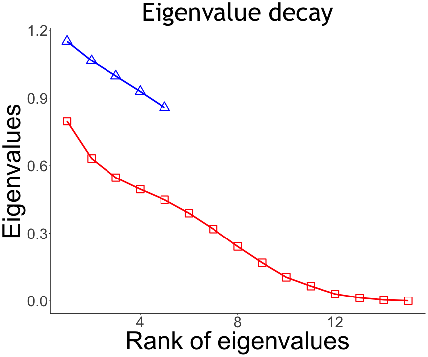
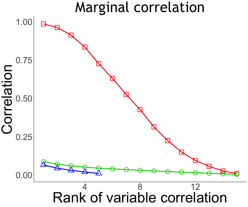
We also compare our method with that of Dai and Barber (2016). More specifically, Dai and Barber (2016) adopted an “expansion first” strategy, which first performs feature expansion 𝚿~(Xj)~𝚿subscript𝑋𝑗\widetilde{\bm{\Psi}}(X_{j}), j=1,,p𝑗1𝑝j=1,\ldots,p, then constructs the knockoffs based on the expanded features. By contrast, we adopt the “knockoffs first” approach, which constructs the knockoffs directly for the variables {Xj}j=1psuperscriptsubscriptsubscript𝑋𝑗𝑗1𝑝\{X_{j}\}_{j=1}^{p}, then performs the random feature expansion on both original variables and their knockoffs. There are two advantages of doing the knockoffs first. First, it ensures a better knockoffs construction and eventually a better statistical power. That is, to construct a good knockoff variable using either the second-order knockoffs or the deep knockoffs, it requires a reasonably slow eigenvalue decay of the covariance 𝚺𝚺\bm{\Sigma}, so that the original variables and their knockoffs are differentiable (Candès et al., 2018). We consider a simulation example replicated 200 times, where the predictors follow a multivariate normal distribution with the zero mean and the identity covariance matrix, n=500,p=5formulae-sequence𝑛500𝑝5n=500,p=5, and we employ the Laplacian kernel with r=3𝑟3r=3. Figure 1(a) shows the eigenvalue decay of the sample covariance matrix (blue line), and the random kernel expansion (red line). It is seen that the former decays more slowly than the latter, and therefore it is better to construct the knockoffs based on the original variables. Second, the “expansion first” leads to larger correlations between the original variables and their knockoffs, compared to the “knockoffs first”, as shown in Figure 1(b), which would in turn make the subsequent group Lasso selection harder. Finally, the “expansion first” is computationally more expensive. This is because the “expansion first” approach requires generating the knockoffs for pr𝑝𝑟pr-dimensional variables, whereas our “knockoffs first” approach only requires generating the knockoffs for p𝑝p-dimensional variables.

Refer to caption
Refer to caption
Figure 1: Comparison between the “expansion first” strategy and the “knockoffs first” strategy. Left panel: the eigenvalue decay of the sample covariance matrix (blue line) and the random kernel expansion (red line). Right panel: the marginal sample correlations between the original variables and the knockoff variables (blue line), between the random kernel expansion and the “expansion first” knockoff variables (red line), and between the random kernel expansion and the “knockoffs first” knockoff variables (green line).

5.2 Varying signal strength, predictor design, and component functions

We first study the performance with the varying signal strength and the predictor distribution.

Multivariate normal predictor distribution
Refer to caption Refer to caption
Mixutre of multivariate normal predictor distribution
Refer to caption Refer to caption
Uniform predictor distribution
Refer to caption Refer to caption
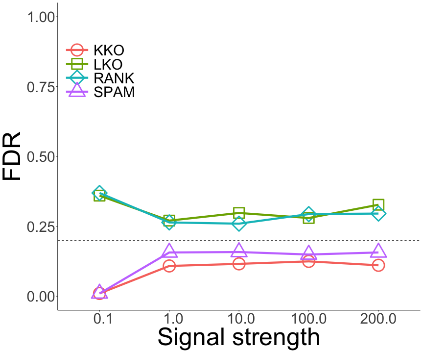
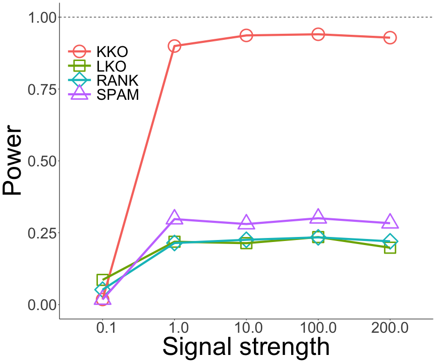
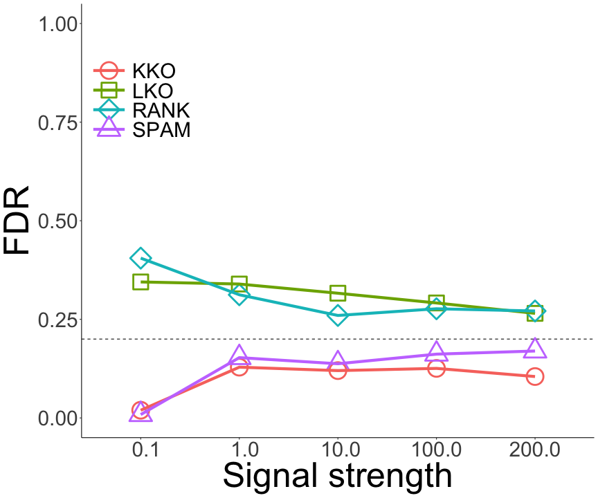
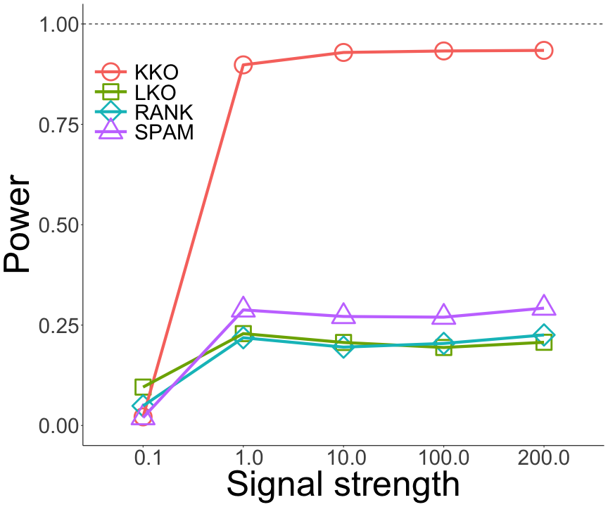
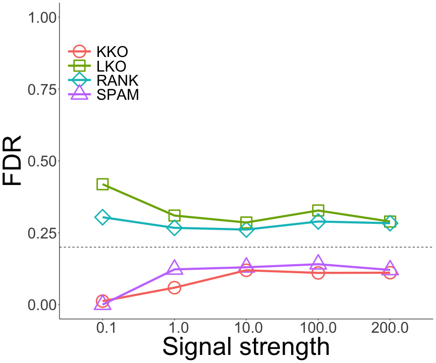
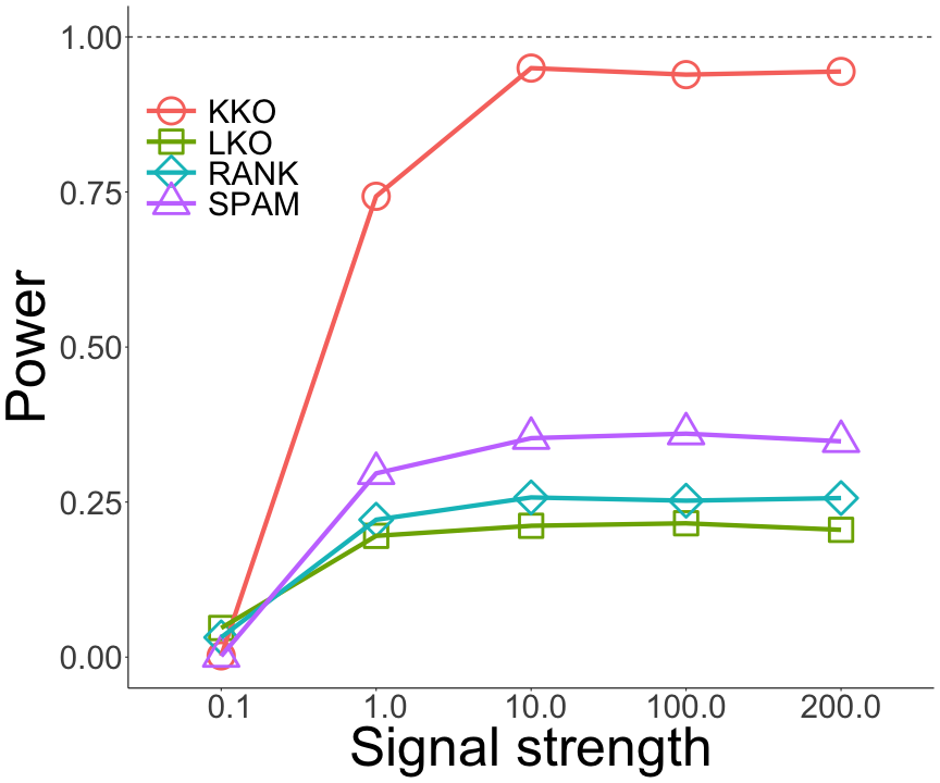
Figure 2: Empirical performance and comparison in terms of FDR and power with the varying signal strength and predictor distribution. Four methods are compared: the nonparametric selection method for sparse additive models (SPAM) of Ravikumar et al. (2009), the linear knockoffs (LKO) of Barber and Candès (2015), the graphical nonlinear knockoffs (RANK) of Fan et al. (2020), and our proposed kernel knockoffs (KKO).

We simulate the response, Y=j𝒮θjfj(Xj)+ϵ𝑌subscript𝑗𝒮subscript𝜃𝑗subscript𝑓𝑗subscript𝑋𝑗italic-ϵY=\sum_{j\in{\mathcal{S}}}\theta_{j}f_{j}(X_{j})+\epsilon, where 𝒮𝒮{\mathcal{S}} is the set of relevant predictors with |𝒮|=10𝒮10|{\mathcal{S}}|=10, and ϵitalic-ϵ\epsilon is a standard normal error. We sample θjsubscript𝜃𝑗\theta_{j} independently from a uniform distribution (θ,θ)𝜃𝜃(-\theta,\theta) for some positive constant θ𝜃\theta. The magnitude of θ𝜃\theta reflects the strength of the signal, and we vary θ={0.1,1,10,100,200}𝜃0.1110100200\theta=\{0.1,1,10,100,200\}. We simulate the predictors independently from three different distributions, a multivariate normal distribution with mean zero and covariance Σij=0.3|ij|subscriptΣ𝑖𝑗superscript0.3𝑖𝑗\Sigma_{ij}=0.3^{|i-j|}, a mixture normal distribution, with an equal probability from three multivariate normal distributions, all with mean zero, and different covariances where Σ1,ij=0.1|ij|subscriptΣ1𝑖𝑗superscript0.1𝑖𝑗\Sigma_{1,ij}=0.1^{|i-j|}, Σ2,ij=0.3|ij|subscriptΣ2𝑖𝑗superscript0.3𝑖𝑗\Sigma_{2,ij}=0.3^{|i-j|}, and Σ3,ij=0.5|ij|subscriptΣ3𝑖𝑗superscript0.5𝑖𝑗\Sigma_{3,ij}=0.5^{|i-j|}, and a uniform [2,2]22[-2,2] distribution. We employ the second-order knockoffs when the predictor distribution is normal, and the deep knockoffs otherwise, to generate the knockoff variables. We first consider a trigonometric polynomial component function, and fix the number of predictors at p=50𝑝50p=50, and the sample size at n=900𝑛900n=900. We later consider other forms of component functions, and different (p,n)𝑝𝑛(p,n).

fj(x)=uj,1sin(cj,1x)+uj,2cos(cj,2x)+uj,3sin2(cj,3x)+uj,4cos2(cj,4x),subscript𝑓𝑗𝑥subscript𝑢𝑗1subscript𝑐𝑗1𝑥subscript𝑢𝑗2subscript𝑐𝑗2𝑥subscript𝑢𝑗3superscript2subscript𝑐𝑗3𝑥subscript𝑢𝑗4superscript2subscript𝑐𝑗4𝑥f_{j}(x)=u_{j,1}\sin(c_{j,1}x)+u_{j,2}\cos(c_{j,2}x)+u_{j,3}\sin^{2}(c_{j,3}x)+u_{j,4}\cos^{2}(c_{j,4}x), (15)

where uj,ksubscript𝑢𝑗𝑘u_{j,k} follows a uniform (1,2)12(1,2) distribution, and cj,ksubscript𝑐𝑗𝑘c_{j,k} follows a uniform (1,10)110(1,10), for k=1,2,3,4𝑘1234k=1,2,3,4. Figure 2 reports the FDR and power over 200 data replications for the four methods with the varying signal strength θ𝜃\theta and three different predictor distributions. It is seen that our method successfully controls the FDR blow the expected level, and at the same time achieves the best power. Besides, the performance is robust with respect to different predictor distributions. By comparison, the alternative methods are much more sensitive in terms of the FDR control, and the powers are consistently lower. Moreover, the linear knockoffs method often fails to control the FDR.

Sin-ratio component function
Refer to caption Refer to caption
Mixture of trigonometric polynomial and sin-raito component function
Refer to caption Refer to caption
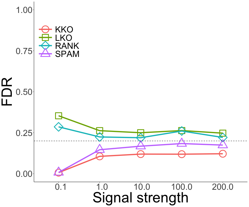
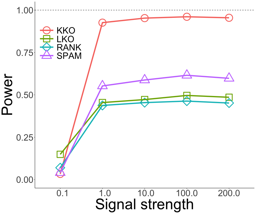
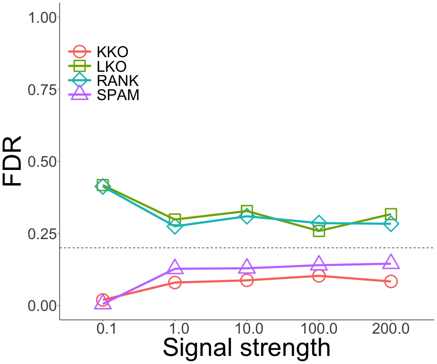
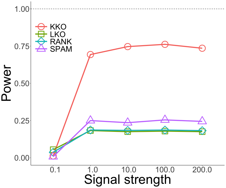
Figure 3: Empirical performance and comparison in terms of FDR and power with the varying signal strength and component function. The same four methods as in Figure 2 are compared.

Next, we consider more forms of component functions. The first is a sin-ratio function,

fj(x)=sin(cj,1x)2sin(cj,2x),subscript𝑓𝑗𝑥subscript𝑐𝑗1𝑥2subscript𝑐𝑗2𝑥f_{j}(x)=\frac{\sin(c_{j,1}x)}{2-\sin(c_{j,2}x)}, (16)

where cj,ksubscript𝑐𝑗𝑘c_{j,k} follows a uniform (1,10)110(1,10) distribution for k=1,2𝑘12k=1,2, and |𝒮|=10𝒮10|{\mathcal{S}}|=10. We note that it is generally more difficult to estimate the sin-ratio function (16) compared to the trigonometric polynomial function (15). The second is a mixed additive model, where we sample the component function with an equal probability from (15) or (16). We fix the predictor distribution as the multivariate normal, p=50𝑝50p=50 and n=900𝑛900n=900. We continue to vary the signal strength θ={0.1,1,10,100,200}𝜃0.1110100200\theta=\{0.1,1,10,100,200\}. Figure 3 reports the FDR and power based on 200 data replications. It is seen again that our method achieves the best power while controlling the FDR under the nominal level for the new component functions.

5.3 Varying sample size and dimension

Next, we investigate the empirical performance with the varying n𝑛n and p𝑝p.

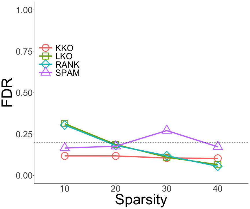
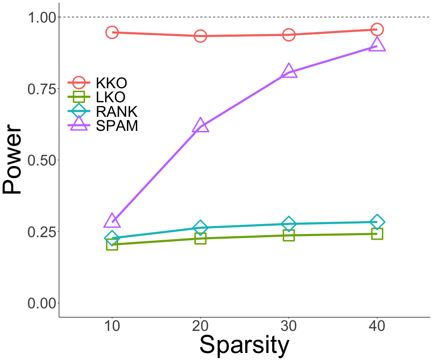
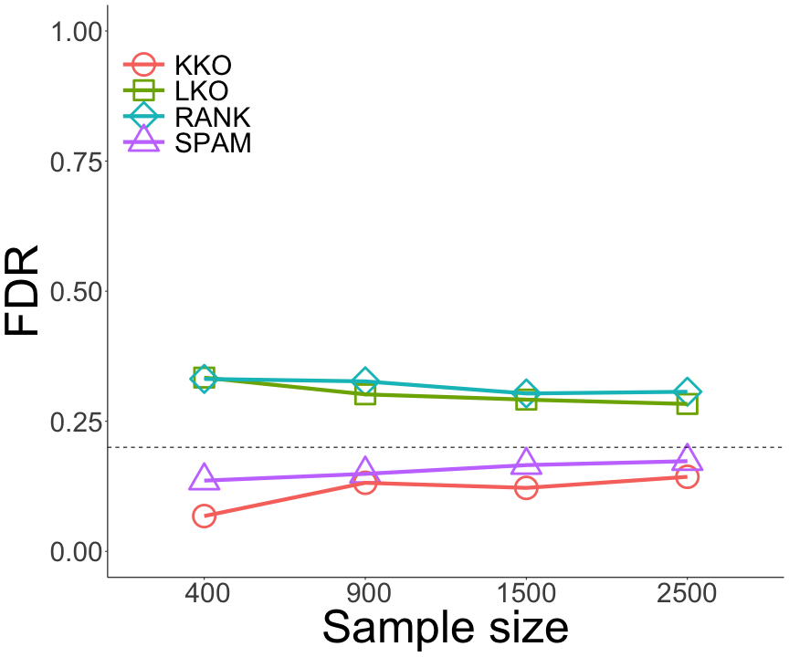
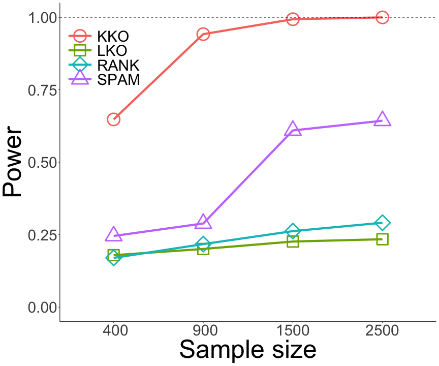
For the varying n𝑛n, we consider the trigonometric polynomial function (15) with p=50,|𝒮|=10,θ=100formulae-sequence𝑝50formulae-sequence𝒮10𝜃100p=50,|{\mathcal{S}}|=10,\theta=100, and the multivariate normal predictor distribution with mean zero and covariance Σij=0.3|ij|subscriptΣ𝑖𝑗superscript0.3𝑖𝑗\Sigma_{ij}=0.3^{|i-j|}. We vary the sample size n={400,900,1500,2500}𝑛40090015002500n=\{400,900,1500,2500\}. Figure 4 reports the FDR and power based on 200 data replications. It is seen that our method successfully control the FDR at all sample sizes, while its power quickly increases as n𝑛n increases, and dominates the powers of all the competitive methods considerably. Besides, both LKO and RANK have an inflated FDR especially when the sample size is small.
Refer to caption
Refer to caption
Figure 4: Empirical performance and comparison in terms of FDR and power with the varying sample size n𝑛n. The same four methods as in Figure 2 are compared.

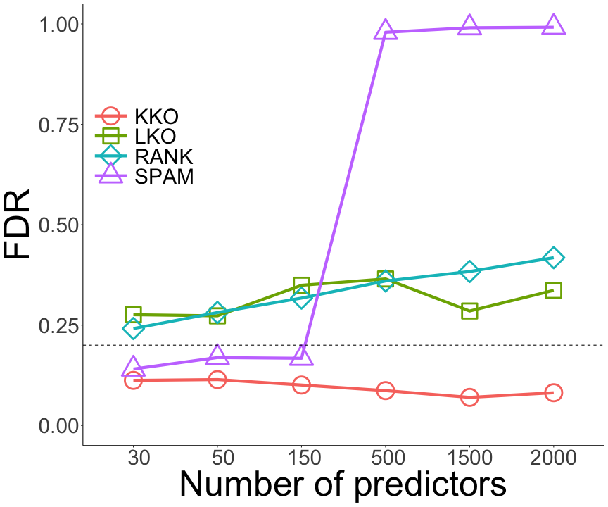
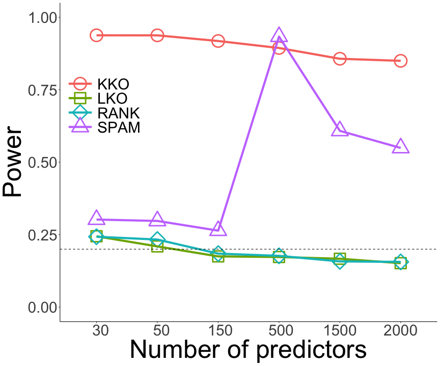
For the varying p𝑝p, we consider the trigonometric polynomial function (15) with n=900,|𝒮|=10,θ=100formulae-sequence𝑛900formulae-sequence𝒮10𝜃100n=900,|{\mathcal{S}}|=10,\theta=100, and the multivariate normal predictor distribution with mean zero and covariance Σij=0.3|ij|subscriptΣ𝑖𝑗superscript0.3𝑖𝑗\Sigma_{ij}=0.3^{|i-j|}. We vary the number of predictors p={30,50,150,500,1500,2000}𝑝305015050015002000p=\{30,50,150,500,1500,2000\}. As such, we have considered both cases that p<n𝑝𝑛p<n and p>n𝑝𝑛p>n. Recall that the proposed method can handle both the low-dimensional and high-dimensional regimes, and the theoretical guarantees in Section 4 are established for both p<n𝑝𝑛p<n and p>n𝑝𝑛p>n. Moreover, for the p>n𝑝𝑛p>n case, we construct the knockoff variables for all the original variables; i.e., we construct the p𝑝p-dimensional knockoffs 𝑿~~𝑿\widetilde{\bm{X}} for the p𝑝p-dimensional 𝑿𝑿\bm{X}. This follows a similar strategy as in Fan et al. (2020), but is different from Barber and Candès (2019), where a precedent step of feature screening is carried out first, and the knockoff variables are constructed only for those selected variables. Our approach avoids to require the sure screening property; see also the discussion in Fan et al. (2020). Figure 5 reports the FDR and power based on 200 data replications. It is seen that our method again achieves the best performance in terms of FDR and power in both regimes. By contrast, LKO and RANK have a low power and inflated FDR. Although SPAM sometimes obtains a power similar to ours, its FDR is much inflated and is far above the nominal level.
Refer to caption
Refer to caption
Figure 5: Empirical performance and comparison in terms of FDR and power with the varying number of predictors p𝑝p in both regimes where p<n𝑝𝑛p<n and p>n𝑝𝑛p>n with n=900𝑛900n=900. The same four methods as in Figure 2 are compared.

5.4 Brain imaging data analysis

We illustrate the proposed method with a brain imaging data analysis to study the Alzheimer’s disease (AD). AD is an irreversible neurodegenerative disorder, and is characterized by progressive impairment of cognitive and memory functions, loss of bodily functions, and ultimately death. It is the leading form of dementia in elderly subjects, and is the sixth leading cause of death in the United States. Over 5.5 million Americans were affected by AD in 2018, and without any effective treatment or prevention, this number is projected to triple by 2050 (Alzheimer’s Association, 2020). Brain atrophy as reflected by brain grey matter cortical thickness is a well-known biomarker for AD. We study a dataset with n=697𝑛697n=697 subjects, each of whom received an anatomical magnetic resonance imaging (MRI) scan that measures cortical thickness. The data is publicly available at http://adni.loni.usc.edu/. The MRI image has been preprocessed by the standard pipeline, and is summarized in the form of a vector of cortical thickness measurements for a set of parcellated brain regions-of-interest. There are p=68𝑝68p=68 regions in total. Brain parcellation is particularly useful to facilitate the interpretation, and has been frequently employed in brain imaging analysis (Fornito et al., 2013; Kang et al., 2016). In addition to the MRI image, for each subject, the data also records a composite cognitive score, which combines numerous tests that assess episodic memory, timed executive function, and global cognition (Donohue et al., 2014). Our goal is to study the association between the composite cognitive score and the vector of brain cortical thickness, and identify individual brain regions with strong associations. A linear model is inadequate to capture such an association, and we turn to the nonparametric additive model instead. We apply the proposed kernel knockoffs selection procedure. As the distribution of the predictors is not necessarily normal, we employ the deep knockoffs machine to generate the knockoff variables. We continue to set the target FDR level at q=0.2𝑞0.2q=0.2.

l-middletemporal l-superiorparietal r-fusiform r-inferiorparietal l-entorhinal
l-fusiform l-inferiorparietal l-precuneus l-superiortemporal r-entorhinal
Table 1: Brain regions identified by the kernel knockoffs selection procedure. “l-” stands for the left hemisphere, and “r-” stands for the right hemisphere.

Table 1 reports the ten brain regions selected by our method. These findings agree with and support the current literature on AD research. Particularly, the middle temporal gyrus is located on the temporal lobe, and is associated with processes of recognition of known faces and accessing word meaning while reading. Middle temporal lobe atrophy is common in AD as well as its prodromal stage, mild cognitive impairment (Visser et al., 2002). The superior parietal lobe is involved with attention, visuospatial perception, and spatial orientation. Damage to the parietal lobe is common in AD, and leads to problems with performing gestures and skilled movements (Pini et al., 2016). The fusiform is linked with various neural pathways related to recognition. The inferior parietal lobe is involved in perception of emotions. The superior temporal gyrus is involved in auditory processing, and has also been implicated as a critical structure in social cognition. Numerous studies have found involvement of these brain regions in the development of AD (Convit et al., 2000; Du et al., 2007; Pini et al., 2016). The precuneus is associated with episodic memory, visuospatial processing, reflections upon self, and aspects of consciousness, and is found to be an AD-signature region (Bakkour et al., 2013). Finally, the entorhinal cortex functions as a hub in a widespread network for memory, navigation and the perception of time. It is found implicated in the early stages of AD, and is one of the most heavily damaged cortices in AD (van Hoesen et al., 1991).

Acknowledgments

The authors thank the Editor, the Associate Editor, and three referees for their constructive comments and insightful suggestions. Li’s research was partially supported by the NSF grant CIF-2102227, and the NIH grants R01AG061303, R01AG062542, and R01AG034570.

References

  • Ahmed et al. (2011) Ahmed, I., Hartikainen, A.-L., Järvelin, M.-R. and Richardson, S. (2011). False discovery rate estimation for stability selection: application to genome-wide association studies. Statistical Applications in Genetics and Molecular Biology 10.
  • Alzheimer’s Association (2020) Alzheimer’s Association (2020). 2020 Alzheimer’s disease facts and figures. Alzheimer’s & Dementia 16 391–460.
  • Aronszajn (1950) Aronszajn, N. (1950). Theory of reproducing kernels. Transactions of the American Mathematical Society 68 337–404.
  • Bach (2017) Bach, F. (2017). On the equivalence between kernel quadrature rules and random feature expansions. The Journal of Machine Learning Research 18 714–751.
  • Bach (2008) Bach, F. R. (2008). Bolasso: model consistent lasso estimation through the bootstrap. In Proceedings of the 25th International Conference on Machine Learning.
  • Bakkour et al. (2013) Bakkour, A., Morris, J. C., Wolk, D. A. and Dickerson, B. C. (2013). The effects of aging and alzheimer’s disease on cerebral cortical anatomy: Specificity and differential relationships with cognition. NeuroImage 76 332–344.
  • Barber and Candès (2015) Barber, R. F. and Candès, E. J. (2015). Controlling the false discovery rate via knockoffs. The Annals of Statistics 43 2055–2085.
  • Barber and Candès (2019) Barber, R. F. and Candès, E. J. (2019). A knockoff filter for high-dimensional selective inference. The Annals of Statistics 47 2504–2537.
  • Barber et al. (2020) Barber, R. F., Candès, E. J. and Samworth, R. J. (2020). Robust inference with knockoffs. The Annals of Statistics 48 1409–1431.
  • Băzăvan et al. (2012) Băzăvan, E. G., Li, F. and Sminchisescu, C. (2012). Fourier Kernel Learning. New York: Springer.
  • Benjamini and Hochberg (1995) Benjamini, Y. and Hochberg, Y. (1995). Controlling the false discovery rate: a practical and powerful approach to multiple testing. Journal of the Royal statistical Society: Series B (Methodological) 57 289–300.
  • Bochner (1934) Bochner, S. (1934). A theorem on fourier-stieltjes integrals. Bulletin of the American Mathematical Society 40 271–276.
  • Cai and Sun (2017) Cai, T. T. and Sun, W. (2017). Large-scale global and simultaneous inference: Estimation and testing in very high dimensions. Annual Review of Economics 9 411–439.
  • Candès et al. (2018) Candès, E., Fan, Y., Janson, L. and Lv, J. (2018). Panning for gold: ‘model-x’ knockoffs for high dimensional controlled variable selection. Journal of the Royal Statistical Society Series B 80 551–577.
  • Convit et al. (2000) Convit, A., de Asis, J. et al. (2000). Atrophy of the medial occipitotemporal, inferior, and middle temporal gyri in non-demented elderly predict decline to alzheimer’s disease. Neurobiology of Aging 21 19–26.
  • Dai and Barber (2016) Dai, R. and Barber, R. (2016). The knockoff filter for fdr control in group-sparse and multitask regression. In International Conference on Machine Learning. PMLR.
  • Dai and Li (2021) Dai, X. and Li, L. (2021). Kernel ordinary differential equations. Journal of the American Statistical Association 1–35.
  • Donohue et al. (2014) Donohue, M. C., Sperling, R. A. and Others (2014). The Preclinical Alzheimer Cognitive Composite: Measuring Amyloid-Related Decline. Journal of the American Medical Association: Neurology 71 961–970.
  • Du et al. (2007) Du, A.-T., Schuff, N., Kramer, J. H., Rosen, H. J., Gorno-Tempini, M. L., Rankin, K., Miller, B. L. and Weiner, M. W. (2007). Different regional patterns of cortical thinning in Alzheimer’s disease and frontotemporal dementia. Brain 130 1159–1166.
  • Dümbgen et al. (2013) Dümbgen, L., Samworth, R. J., Schuhmacher, D. et al. (2013). Stochastic search for semiparametric linear regression models. In From Probability to Statistics and Back: High-Dimensional Models and Processes–A Festschrift in Honor of Jon A. Wellner. Institute of Mathematical Statistics, 78–90.
  • Efron et al. (2001) Efron, B., Tibshirani, R., Storey, J. D. and Tusher, V. (2001). Empirical bayes analysis of a microarray experiment. Journal of the American Statistical Association 96 1151–1160.
  • Fan et al. (2020) Fan, Y., Demirkaya, E., Li, G. and Lv, J. (2020). Rank: large-scale inference with graphical nonlinear knockoffs. Journal of the American Statistical Association 115 362–379.
  • Fornito et al. (2013) Fornito, A., Zalesky, A. and Breakspear, M. (2013). Graph analysis of the human connectome: Promise, progress, and pitfalls. NeuroImage 80 426–444.
  • Hastie and Tibshirani (1990) Hastie, T. J. and Tibshirani, R. J. (1990). Generalized Additive Models, vol. 43. London: Chapman and Hall.
  • He et al. (2016) He, K., Li, Y., Zhu, J., Liu, H., Lee, J. E., Amos, C. I., Hyslop, T., Jin, J., Lin, H. and Wei, Q. (2016). Component-wise gradient boosting and false discovery control in survival analysis with high-dimensional covariates. Bioinformatics 32 50–57.
  • Huang et al. (2010) Huang, J., Horowitz, J. L. and Wei, F. (2010). Variable selection in nonparametric additive models. Annals of Statistics 38 2282.
  • Kang et al. (2016) Kang, J., Bowman, F. D., Mayberg, H. and Liu, H. (2016). A depression network of functionally connected regions discovered via multi-attribute canonical correlation graphs. NeuroImage 141 431–441.
  • Koltchinskii and Yuan (2010) Koltchinskii, V. and Yuan, M. (2010). Sparsity in multiple kernel learning. The Annals of Statistics 38 3660–3695.
  • Li et al. (2005) Li, L., Cook, R. D. and Nachtsheim, C. J. (2005). Model-free variable selection. Journal of the Royal Statistical Society. Series B (Statistical Methodology) 67 285–299.
  • Li et al. (2013) Li, S., Hsu, L., Peng, J. and Wang, P. (2013). Bootstrap inference for network construction with an application to a breast cancer microarray study. The Annals of Applied Statistics 7 391.
  • Lin and Zhang (2006) Lin, Y. and Zhang, H. H. (2006). Component selection and smoothing in multivariate nonparametric regression. The Annals of Statistics 34 2272–2297.
  • Loh and Wainwright (2012) Loh, P.-L. and Wainwright, M. J. (2012). High-dimensional regression with noisy and missing data: Provable guarantees with nonconvexity. Annals of Statistics 40 1637–1664.
  • Meier et al. (2009) Meier, L., Van de Geer, S. and Bühlmann, P. (2009). High-dimensional additive modeling. The Annals of Statistics 37 3779–3821.
  • Meinshausen and Bühlmann (2010) Meinshausen, N. and Bühlmann, P. (2010). Stability selection. Journal of the Royal Statistical Society: Series B (Statistical Methodology) 72 417–473.
  • Mercer (1909) Mercer, J. (1909). Functions of positive and negative type and their connection with the theory of integral equations. Philosophical Transactions of the Royal Society, London A 415–446.
  • Miller (2002) Miller, A. (2002). Subset Selection in Regression. CRC Press.
  • Pini et al. (2016) Pini, L., Pievani, M., Bocchetta, M., Altomare, D., Bosco, P., Cavedo, E., Galluzzi, S., Marizzoni, M. and Frisoni, G. B. (2016). Brain atrophy in alzheimer’s disease and aging. Aging Research Reviews 30 25–48. Brain Imaging and Aging.
  • Rahimi and Recht (2007) Rahimi, A. and Recht, B. (2007). Random features for large-scale kernel machines. Advances in Neural Information Processing systems 20 1177–1184.
  • Raskutti et al. (2012) Raskutti, G., J Wainwright, M. and Yu, B. (2012). Minimax-optimal rates for sparse additive models over kernel classes via convex programming. Journal of Machine Learning Research 13.
  • Raskutti et al. (2011) Raskutti, G., Wainwright, M. J. and Yu, B. (2011). Minimax rates of estimation for high-dimensional linear regression over qsubscript𝑞\ell_{q}-balls. IEEE Transactions on Information Theory 57 6976–6994.
  • Ravikumar et al. (2009) Ravikumar, P., Lafferty, J., Liu, H. and Wasserman, L. (2009). Sparse additive models. Journal of the Royal Statistical Society: Series B (Statistical Methodology) 71 1009–1030.
  • Ravikumar et al. (2010) Ravikumar, P., Wainwright, M. J. and Lafferty, J. D. (2010). High-dimensional ising model selection using l1subscript𝑙1l_{1}-regularized logistic regression. The Annals of Statistics 38 1287–1319.
  • Ren et al. (2020) Ren, Z., Wei, Y. and Candès, E. (2020). Derandomizing knockoffs. arXiv preprint arXiv:2012.02717 .
  • Romano et al. (2019) Romano, Y., Sesia, M. and Candès, E. (2019). Deep knockoffs. Journal of the American Statistical Association 1–12.
  • Rudi and Rosasco (2017) Rudi, A. and Rosasco, L. (2017). Generalization properties of learning with random features. In NIPS.
  • Schölkopf and Smola (2002) Schölkopf, B. and Smola, A. J. (2002). Learning with Kernels: Support Vector Machines, Regularization, Optimization, and Beyond. MIT press.
  • Stone (1985) Stone, C. J. (1985). Additive regression and other nonparametric models. The Annals of Statistics 689–705.
  • Storey (2007) Storey, J. D. (2007). The optimal discovery procedure: a new approach to simultaneous significance testing. Journal of the Royal Statistical Society: Series B (Statistical Methodology) 69 347–368.
  • Su et al. (2017) Su, W., Bogdan, M. and Candes, E. (2017). False discoveries occur early on the lasso path. The Annals of statistics 2133–2150.
  • Sun and Cai (2007) Sun, W. and Cai, T. T. (2007). Oracle and adaptive compound decision rules for false discovery rate control. Journal of the American Statistical Association 102 901–912.
  • Sun and Cai (2009) Sun, W. and Cai, T. T. (2009). Large-scale multiple testing under dependence. Journal of the Royal Statistical Society: Series B (Statistical Methodology) 71 393–424.
  • van de Geer (2000) van de Geer, S. (2000). Empirical Processes in M𝑀M-Estimation. Cambridge University Press.
  • van de Geer (2002) van de Geer, S. A. (2002). On hoeffding’s inequality for dependent random variables. In Empirical process techniques for dependent data. Springer, 161–169.
  • van Hoesen et al. (1991) van Hoesen, G. W., Hyman, B. T. and Damasio, A. R. (1991). Entorhinal cortex pathology in alzheimer’s disease. Hippocampus 1 1–8.
  • Visser et al. (2002) Visser, P. J., Verhey, F. R. J., Hofman, P. A. M., Scheltens, P. and Jolles, J. (2002). Medial temporal lobe atrophy predicts alzheimer’s disease in patients with minor cognitive impairment. Journal of Neurology, Neurosurgery & Psychiatry 72 491–497.
  • Wahba (1990) Wahba, G. (1990). Spline Models for Observational Data. SIAM.
  • Wahba et al. (1995) Wahba, G., Wang, Y., Gu, C., Klein, R. and Klein, B. (1995). Smoothing spline anova for exponential families, with application to the wisconsin epidemiological study of diabetic retinopathy. The Annals of Statistics 23 1865–1895.
  • Weinstein et al. (2020) Weinstein, A., Su, W. J., Bogdan, M., Barber, R. F. and Candès, E. J. (2020). A power analysis for knockoffs with the lasso coefficient-difference statistic. arXiv preprint arXiv:2007.15346 .
  • Wood (2017) Wood, S. N. (2017). Generalized Additive Models: An Introduction With R. CRC press.
  • Wu et al. (2007) Wu, Y., Boos, D. D. and Stefanski, L. A. (2007). Controlling variable selection by the addition of pseudovariables. Journal of the American Statistical Association 102 235–243.
  • Yuan and Zhou (2016) Yuan, M. and Zhou, D.-X. (2016). Minimax optimal rates of estimation in high dimensional additive models. Annals of Statistics 44 2564–2593.
  • Zhao and Yu (2006) Zhao, P. and Yu, B. (2006). On model selection consistency of lasso. Journal of Machine Learning Research 7 2541–2563.

Appendix A Proofs

A.1 Proof of Proposition 1

Proof.

Recall that, in the nonparametric additive model (1), the conditional distribution of Y𝑌Y given 𝑿𝒳p𝑿superscript𝒳𝑝\bm{X}\in{\mathcal{X}}^{p} follows a normal distribution, i.e.,

pY|𝑿(y|x1,,xp)=1σ2πexp{12σ2[yj=1pfj(xj)]2}.subscript𝑝conditional𝑌𝑿conditional𝑦subscript𝑥1subscript𝑥𝑝1𝜎2𝜋12superscript𝜎2superscriptdelimited-[]𝑦superscriptsubscript𝑗1𝑝subscript𝑓𝑗subscript𝑥𝑗2p_{Y|\bm{X}}(y|x_{1},\ldots,x_{p})=\frac{1}{\sigma\sqrt{2\pi}}\exp\left\{-\frac{1}{2\sigma^{2}}\left[y-\sum_{j=1}^{p}f_{j}(x_{j})\right]^{2}\right\}.

Let 𝒙j={x1,,xp}\{xj}subscript𝒙𝑗\subscript𝑥1subscript𝑥𝑝subscript𝑥𝑗\bm{x}_{-j}=\{x_{1},\ldots,x_{p}\}\backslash\{x_{j}\}. Note that

pY,Xj|𝑿j(y,xj|𝒙j)=pY|Xj,𝑿j(y|xj,𝒙j)pXj|𝑿j(xj|𝒙j).subscript𝑝𝑌conditionalsubscript𝑋𝑗subscript𝑿𝑗𝑦conditionalsubscript𝑥𝑗subscript𝒙𝑗subscript𝑝conditional𝑌subscript𝑋𝑗subscript𝑿𝑗conditional𝑦subscript𝑥𝑗subscript𝒙𝑗subscript𝑝conditionalsubscript𝑋𝑗subscript𝑿𝑗conditionalsubscript𝑥𝑗subscript𝒙𝑗\displaystyle p_{Y,X_{j}|\bm{X}_{-j}}(y,x_{j}|\bm{x}_{-j})=p_{Y|X_{j},\bm{X}_{-j}}(y|x_{j},\bm{x}_{-j})p_{X_{j}|\bm{X}_{-j}}(x_{j}|\bm{x}_{-j}).

Now if fj=0subscript𝑓𝑗0f_{j}=0 for j{1,,p}𝑗1𝑝j\in\{1,\ldots,p\}, then

pY|Xj,𝑿j(y|xj,𝒙j)subscript𝑝conditional𝑌subscript𝑋𝑗subscript𝑿𝑗conditional𝑦subscript𝑥𝑗subscript𝒙𝑗\displaystyle p_{Y|X_{j},\bm{X}_{-j}}(y|x_{j},\bm{x}_{-j}) =pY|𝑿j(y|𝒙j).absentsubscript𝑝conditional𝑌subscript𝑿𝑗conditional𝑦subscript𝒙𝑗\displaystyle=p_{Y|\bm{X}_{-j}}(y|\bm{x}_{-j}).

Henceforth,

pY,Xj|𝑿j(y,xj|𝒙j)=pY|𝑿j(y|𝒙j)pXj|𝑿j(xj|𝒙j).subscript𝑝𝑌conditionalsubscript𝑋𝑗subscript𝑿𝑗𝑦conditionalsubscript𝑥𝑗subscript𝒙𝑗subscript𝑝conditional𝑌subscript𝑿𝑗conditional𝑦subscript𝒙𝑗subscript𝑝conditionalsubscript𝑋𝑗subscript𝑿𝑗conditionalsubscript𝑥𝑗subscript𝒙𝑗\displaystyle p_{Y,X_{j}|\bm{X}_{-j}}(y,x_{j}|\bm{x}_{-j})=p_{Y|\bm{X}_{-j}}(y|\bm{x}_{-j})p_{X_{j}|\bm{X}_{-j}}(x_{j}|\bm{x}_{-j}). (17)

That is, the conditional distribution pY,Xj|𝑿j(y,xj|𝒙j)subscript𝑝𝑌conditionalsubscript𝑋𝑗subscript𝑿𝑗𝑦conditionalsubscript𝑥𝑗subscript𝒙𝑗p_{Y,X_{j}|\bm{X}_{-j}}(y,x_{j}|\bm{x}_{-j}) factorizes. Consequently, YXj|𝑿jperpendicular-toabsentperpendicular-to𝑌conditionalsubscript𝑋𝑗subscript𝑿𝑗Y\mathchoice{\mathrel{\hbox to0.0pt{$\displaystyle\perp$\hss}\mkern 2.0mu{\displaystyle\perp}}}{\mathrel{\hbox to0.0pt{$\textstyle\perp$\hss}\mkern 2.0mu{\textstyle\perp}}}{\mathrel{\hbox to0.0pt{$\scriptstyle\perp$\hss}\mkern 2.0mu{\scriptstyle\perp}}}{\mathrel{\hbox to0.0pt{$\scriptscriptstyle\perp$\hss}\mkern 2.0mu{\scriptscriptstyle\perp}}}X_{j}|\bm{X}_{-j} and thus, j𝒮𝑗superscript𝒮perpendicular-toj\in{\mathcal{S}}^{\perp}.

On the other hand, suppose that j𝒮𝑗superscript𝒮perpendicular-toj\in{\mathcal{S}}^{\perp}. By definition, YXj|𝑿jperpendicular-toabsentperpendicular-to𝑌conditionalsubscript𝑋𝑗subscript𝑿𝑗Y\mathchoice{\mathrel{\hbox to0.0pt{$\displaystyle\perp$\hss}\mkern 2.0mu{\displaystyle\perp}}}{\mathrel{\hbox to0.0pt{$\textstyle\perp$\hss}\mkern 2.0mu{\textstyle\perp}}}{\mathrel{\hbox to0.0pt{$\scriptstyle\perp$\hss}\mkern 2.0mu{\scriptstyle\perp}}}{\mathrel{\hbox to0.0pt{$\scriptscriptstyle\perp$\hss}\mkern 2.0mu{\scriptscriptstyle\perp}}}X_{j}|\bm{X}_{-j}. Then the likelihood pY,Xj|𝑿j(y,xj|𝒙j)subscript𝑝𝑌conditionalsubscript𝑋𝑗subscript𝑿𝑗𝑦conditionalsubscript𝑥𝑗subscript𝒙𝑗p_{Y,X_{j}|\bm{X}_{-j}}(y,x_{j}|\bm{x}_{-j}) need to factorize and satisfy (17). Note that pY,Xj|𝑿j(y,xj|𝒙j)subscript𝑝𝑌conditionalsubscript𝑋𝑗subscript𝑿𝑗𝑦conditionalsubscript𝑥𝑗subscript𝒙𝑗p_{Y,X_{j}|\bm{X}_{-j}}(y,x_{j}|\bm{x}_{-j}) has an interaction term,

1σ2πexp(1σ2fj(xj)(yk=1;kjpfk(xk))).1𝜎2𝜋1superscript𝜎2subscript𝑓𝑗subscript𝑥𝑗𝑦superscriptsubscriptformulae-sequence𝑘1𝑘𝑗𝑝subscript𝑓𝑘subscript𝑥𝑘\frac{1}{\sigma\sqrt{2\pi}}\exp\left(\frac{1}{\sigma^{2}}f_{j}(x_{j})\left(y-\sum_{k=1;k\neq j}^{p}f_{k}(x_{k})\right)\right). (18)

Since pY,Xj|𝑿j(y,xj|𝒙j)subscript𝑝𝑌conditionalsubscript𝑋𝑗subscript𝑿𝑗𝑦conditionalsubscript𝑥𝑗subscript𝒙𝑗p_{Y,X_{j}|\bm{X}_{-j}}(y,x_{j}|\bm{x}_{-j}) satisfies (17), (18) needs to be a constant that is independent of 𝒙𝒙\bm{x} and y𝑦y. Under Assumption 1, this is true only if fj=0subscript𝑓𝑗0f_{j}=0. This completes the proof of Proposition 1. ∎

A.2 Proof of Theorem 1

Proof.

Recall that the selected set 𝒮^(I)^𝒮𝐼\widehat{\mathcal{S}}(I) is obtained by (8). Then 𝒮^(I)^𝒮𝐼\widehat{\mathcal{S}}(I) is a function of

𝚺(I)[𝚿(xi1,1)T𝚿(xi1,p)T𝚿(x~i1,1)T𝚿(x~i1,p)T𝚿(xi|I|,1)T𝚿(xi|I|,p)T𝚿(x~i|I|,1)T𝚿(x~i|I|,p)T]|I|×2pr,𝚺𝐼matrix𝚿superscriptsubscript𝑥subscript𝑖11T𝚿superscriptsubscript𝑥subscript𝑖1𝑝T𝚿superscriptsubscript~𝑥subscript𝑖11T𝚿superscriptsubscript~𝑥subscript𝑖1𝑝Tmissing-subexpressionmissing-subexpression𝚿superscriptsubscript𝑥subscript𝑖𝐼1T𝚿superscriptsubscript𝑥subscript𝑖𝐼𝑝T𝚿superscriptsubscript~𝑥subscript𝑖𝐼1T𝚿superscriptsubscript~𝑥subscript𝑖𝐼𝑝Tsuperscript𝐼2𝑝𝑟\bm{\Sigma}(I)\equiv\begin{bmatrix}\bm{\Psi}(x_{i_{1},1})^{\mbox{\tiny{\sf T}}}&\cdots&\bm{\Psi}(x_{i_{1},p})^{\mbox{\tiny{\sf T}}}&\bm{\Psi}(\widetilde{x}_{i_{1},1})^{\mbox{\tiny{\sf T}}}&\cdots&\bm{\Psi}(\widetilde{x}_{i_{1},p})^{\mbox{\tiny{\sf T}}}\\ \vdots&&\vdots&\vdots&&\vdots\\ \bm{\Psi}(x_{i_{|I|},1})^{\mbox{\tiny{\sf T}}}&\cdots&\bm{\Psi}(x_{i_{|I|},p})^{\mbox{\tiny{\sf T}}}&\bm{\Psi}(\widetilde{x}_{i_{|I|},1})^{\mbox{\tiny{\sf T}}}&\cdots&\bm{\Psi}(\widetilde{x}_{i_{|I|},p})^{\mbox{\tiny{\sf T}}}\end{bmatrix}\in\mathbb{R}^{|I|\times 2pr}, (19)

where I=(i1,,i|I|)𝐼subscript𝑖1subscript𝑖𝐼I=(i_{1},\ldots,i_{|I|}), and the feature vectors 𝚿(xi,j)=[ψ1(xi,j),,ψr(xi,j)]Tr𝚿subscript𝑥𝑖𝑗superscriptsubscript𝜓1subscript𝑥𝑖𝑗subscript𝜓𝑟subscript𝑥𝑖𝑗Tsuperscript𝑟\bm{\Psi}(x_{i,j})=\left[\psi_{1}(x_{i,j}),\ldots,\psi_{r}(x_{i,j})\right]^{\mbox{\tiny{\sf T}}}\in\mathbb{R}^{r}, 𝚿(x~i,j)𝚿subscript~𝑥𝑖𝑗\bm{\Psi}(\widetilde{x}_{i,j}) =[ψ1(x~i,j),,ψr(x~i,j)]Trabsentsuperscriptsubscript𝜓1subscript~𝑥𝑖𝑗subscript𝜓𝑟subscript~𝑥𝑖𝑗Tsuperscript𝑟=\left[\psi_{1}(\widetilde{x}_{i,j}),\ldots,\psi_{r}(\widetilde{x}_{i,j})\right]^{\mbox{\tiny{\sf T}}}\in\mathbb{R}^{r} with i=i1,,i|I|𝑖subscript𝑖1subscript𝑖𝐼i=i_{1},\ldots,i_{|I|}, and j=1,,p𝑗1𝑝j=1,\ldots,p. Moreover, 𝒮^(I)^𝒮𝐼\widehat{\mathcal{S}}(I) is a function of the response vector 𝒚(I)=(y1,,y|I|)T|I|𝒚𝐼superscriptsubscript𝑦1subscript𝑦𝐼Tsuperscript𝐼\bm{y}(I)=(y_{1},\ldots,y_{|I|})^{\mbox{\tiny{\sf T}}}\in\mathbb{R}^{|I|}. Since the importance score Δj=Π^jΠ^j+psubscriptΔ𝑗subscript^Π𝑗subscript^Π𝑗𝑝\Delta_{j}=\widehat{\Pi}_{j}-\widehat{\Pi}_{j+p} with Π^j={j𝒮^(I)}subscript^Π𝑗𝑗^𝒮𝐼\widehat{\Pi}_{j}=\mathbb{P}\{j\in\widehat{\mathcal{S}}(I)\}, ΔjsubscriptΔ𝑗\Delta_{j} is a function of 𝚺(I)𝚺𝐼\bm{\Sigma}(I) and 𝒚(I)𝒚𝐼\bm{y}(I). That is,

Δj=Δj(𝚺(I),𝒚(I)).subscriptΔ𝑗subscriptΔ𝑗𝚺𝐼𝒚𝐼\Delta_{j}=\Delta_{j}\left(\bm{\Sigma}(I),\bm{y}(I)\right).

Next, we complete the proof of Theorem 1 in three steps.

Step 1.

We show the flip sign property that, for any 𝒜1{1,,p}subscript𝒜11𝑝{\mathcal{A}}_{1}\subseteq\{1,\ldots,p\}, the importance score satisfies that,

Δj({𝚺(I)}swap(𝒜1),𝒚(I))={Δj(𝚺(I),𝒚(I)),j𝒜1,Δj(𝚺(I),𝒚(I)),j𝒜1,subscriptΔ𝑗subscript𝚺𝐼swapsubscript𝒜1𝒚𝐼casessubscriptΔ𝑗𝚺𝐼𝒚𝐼𝑗subscript𝒜1subscriptΔ𝑗𝚺𝐼𝒚𝐼𝑗subscript𝒜1\Delta_{j}\left(\{\bm{\Sigma}(I)\}_{\text{swap}({\mathcal{A}}_{1})},\bm{y}(I)\right)=\begin{cases}\Delta_{j}\left(\bm{\Sigma}(I),\bm{y}(I)\right),&j\not\in{\mathcal{A}}_{1},\\ -\Delta_{j}\left(\bm{\Sigma}(I),\bm{y}(I)\right),&j\in{\mathcal{A}}_{1},\end{cases} (20)

where swap(j)swap𝑗\text{swap}(j) is an operator that swaps the submatrix

[𝚿(xi1,j)T𝚿(xi|I|,j)T]|I|×r with [𝚿(x~i1,j)T𝚿(x~i|I|,j)T]|I|×rformulae-sequencematrix𝚿superscriptsubscript𝑥subscript𝑖1𝑗T𝚿superscriptsubscript𝑥subscript𝑖𝐼𝑗Tsuperscript𝐼𝑟 with matrix𝚿superscriptsubscript~𝑥subscript𝑖1𝑗T𝚿superscriptsubscript~𝑥subscript𝑖𝐼𝑗Tsuperscript𝐼𝑟\begin{bmatrix}\bm{\Psi}(x_{i_{1},j})^{\mbox{\tiny{\sf T}}}\\ \vdots\\ \bm{\Psi}(x_{i_{|I|},j})^{\mbox{\tiny{\sf T}}}\end{bmatrix}\in\mathbb{R}^{|I|\times r}\quad\text{ with }\quad\begin{bmatrix}\bm{\Psi}(\widetilde{x}_{i_{1},j})^{\mbox{\tiny{\sf T}}}\\ \vdots\\ \bm{\Psi}(\widetilde{x}_{i_{|I|},j})^{\mbox{\tiny{\sf T}}}\end{bmatrix}\in\mathbb{R}^{|I|\times r}

Note that after the operation swap(𝒜1)swapsubscript𝒜1\text{swap}({\mathcal{A}}_{1}), the selection probability Π^jnewsuperscriptsubscript^Π𝑗new\widehat{\Pi}_{j}^{\text{new}} obtained by (9) satisfies

Π^jnew={Π^jj𝒜1,Π^j+p or Π^jpj𝒜1,subscriptsuperscript^Πnew𝑗casessubscript^Π𝑗𝑗subscript𝒜1subscript^Π𝑗𝑝 or subscript^Π𝑗𝑝𝑗subscript𝒜1\widehat{\Pi}^{\text{new}}_{j}=\begin{cases}\widehat{\Pi}_{j}\quad&j\not\in{\mathcal{A}}_{1},\\ \widehat{\Pi}_{j+p}\text{ or }\widehat{\Pi}_{j-p}\quad&j\in{\mathcal{A}}_{1},\end{cases}

Since Δj=Π^jΠ^j+psubscriptΔ𝑗subscript^Π𝑗subscript^Π𝑗𝑝\Delta_{j}=\widehat{\Pi}_{j}-\widehat{\Pi}_{j+p} is an asymmetric function, we have (20) holds.

Step 2.

We show that the exchangeability holds, in that

({𝚺(I)}swap(𝒜2),𝒚(I))=𝑑(𝚺(I),𝒚(I)),subscript𝚺𝐼swapsubscript𝒜2𝒚𝐼𝑑𝚺𝐼𝒚𝐼\left(\{\bm{\Sigma}(I)\}_{\text{swap}({\mathcal{A}}_{2})},\bm{y}(I)\right)\overset{d}{=}\left(\bm{\Sigma}(I),\bm{y}(I)\right), (21)

where 𝒜2𝒮subscript𝒜2superscript𝒮perpendicular-to{\mathcal{A}}_{2}\subseteq{\mathcal{S}}^{\perp} is any set of null variables. Without loss of generality, assume that 𝒜2={1,2,,|𝒮|}subscript𝒜212superscript𝒮perpendicular-to{\mathcal{A}}_{2}=\{1,2,\ldots,|{\mathcal{S}}^{\perp}|\}. Since the rows of (𝚺(I),𝒚(I))|I|×(2pr+1)𝚺𝐼𝒚𝐼superscript𝐼2𝑝𝑟1(\bm{\Sigma}(I),\bm{y}(I))\in\mathbb{R}^{|I|\times(2pr+1)} are independent, it suffices to show that

({𝚿2p(𝑿)T}swap(𝒜2),Y)=𝑑(𝚿2p(𝑿)T,Y),subscriptsubscript𝚿2𝑝superscript𝑿Tswapsubscript𝒜2𝑌𝑑subscript𝚿2𝑝superscript𝑿T𝑌\left(\{\bm{\Psi}_{2p}(\bm{X})^{\mbox{\tiny{\sf T}}}\}_{\text{swap}({\mathcal{A}}_{2})},Y\right)\overset{d}{=}\left(\bm{\Psi}_{2p}(\bm{X})^{\mbox{\tiny{\sf T}}},Y\right),

where 𝚿2p(𝑿)Tsubscript𝚿2𝑝superscript𝑿T\bm{\Psi}_{2p}(\bm{X})^{\mbox{\tiny{\sf T}}} is a row of the matrix 𝚺(I)𝚺𝐼\bm{\Sigma}(I), i.e.,

𝚿2p(𝑿)T[𝚿(X1)T,,𝚿(Xp)T,𝚿(X~1)T,,𝚿(X~p)T]1×2pr.subscript𝚿2𝑝superscript𝑿T𝚿superscriptsubscript𝑋1T𝚿superscriptsubscript𝑋𝑝T𝚿superscriptsubscript~𝑋1T𝚿superscriptsubscript~𝑋𝑝Tsuperscript12𝑝𝑟\bm{\Psi}_{2p}(\bm{X})^{\mbox{\tiny{\sf T}}}\equiv\left[\bm{\Psi}(X_{1})^{\mbox{\tiny{\sf T}}},\ldots,\bm{\Psi}(X_{p})^{\mbox{\tiny{\sf T}}},\bm{\Psi}(\widetilde{X}_{1})^{\mbox{\tiny{\sf T}}},\ldots,\bm{\Psi}(\widetilde{X}_{p})^{\mbox{\tiny{\sf T}}}\right]\in\mathbb{R}^{1\times 2pr}.

Furthermore, since {𝚿2pT(𝑿)}swap(𝒜2)=𝑑𝚿2pT(𝑿)subscriptsubscriptsuperscript𝚿T2𝑝𝑿swapsubscript𝒜2𝑑subscriptsuperscript𝚿T2𝑝𝑿\{\bm{\Psi}^{\mbox{\tiny{\sf T}}}_{2p}(\bm{X})\}_{\text{swap}({\mathcal{A}}_{2})}\overset{d}{=}\bm{\Psi}^{\mbox{\tiny{\sf T}}}_{2p}(\bm{X}), we only need to establish that

Y|{𝚿2pT(𝑿)}swap(𝒜2)=𝑑Y|𝚿2pT(𝑿).𝑌subscriptsubscriptsuperscript𝚿T2𝑝𝑿swapsubscript𝒜2𝑑𝑌subscriptsuperscript𝚿T2𝑝𝑿Y|\{\bm{\Psi}^{\mbox{\tiny{\sf T}}}_{2p}(\bm{X})\}_{\text{swap}({\mathcal{A}}_{2})}\overset{d}{=}Y|\bm{\Psi}^{\mbox{\tiny{\sf T}}}_{2p}(\bm{X}). (22)

Let 𝚿p(𝑿~)=[𝚿(X~1)T,,𝚿(X~p)T]Tprsubscript𝚿𝑝~𝑿superscript𝚿superscriptsubscript~𝑋1T𝚿superscriptsubscript~𝑋𝑝TTsuperscript𝑝𝑟\bm{\Psi}_{p}(\widetilde{\bm{X}})=\left[\bm{\Psi}(\widetilde{X}_{1})^{\mbox{\tiny{\sf T}}},\ldots,\bm{\Psi}(\widetilde{X}_{p})^{\mbox{\tiny{\sf T}}}\right]^{\mbox{\tiny{\sf T}}}\in\mathbb{R}^{pr} and 𝚿p(𝑿)=[𝚿(X1)T,,𝚿(Xp)T]Tprsubscript𝚿𝑝𝑿superscript𝚿superscriptsubscript𝑋1T𝚿superscriptsubscript𝑋𝑝TTsuperscript𝑝𝑟\bm{\Psi}_{p}(\bm{X})=\left[\bm{\Psi}(X_{1})^{\mbox{\tiny{\sf T}}},\ldots,\bm{\Psi}(X_{p})^{\mbox{\tiny{\sf T}}}\right]^{\mbox{\tiny{\sf T}}}\in\mathbb{R}^{pr}. Here for each j=1,,p𝑗1𝑝j=1,\ldots,p, 𝚿(Xj)=[ψ1(Xj),,ψr(Xj)]Tr𝚿subscript𝑋𝑗superscriptsubscript𝜓1subscript𝑋𝑗subscript𝜓𝑟subscript𝑋𝑗Tsuperscript𝑟\bm{\Psi}(X_{j})=\left[\psi_{1}(X_{j}),\ldots,\psi_{r}(X_{j})\right]^{\mbox{\tiny{\sf T}}}\in\mathbb{R}^{r}, where ψk(Xj)1subscript𝜓𝑘subscript𝑋𝑗subscript1\psi_{k}(X_{j})\in{\mathcal{H}}_{1}, with k=1,,r𝑘1𝑟k=1,\ldots,r. Since Y𝑿~|𝑿perpendicular-toabsentperpendicular-to𝑌conditional~𝑿𝑿Y\mathchoice{\mathrel{\hbox to0.0pt{$\displaystyle\perp$\hss}\mkern 2.0mu{\displaystyle\perp}}}{\mathrel{\hbox to0.0pt{$\textstyle\perp$\hss}\mkern 2.0mu{\textstyle\perp}}}{\mathrel{\hbox to0.0pt{$\scriptstyle\perp$\hss}\mkern 2.0mu{\scriptstyle\perp}}}{\mathrel{\hbox to0.0pt{$\scriptscriptstyle\perp$\hss}\mkern 2.0mu{\scriptscriptstyle\perp}}}\widetilde{\bm{X}}|\bm{X}, by Proposition 1, we have that,

Y𝚿p(𝑿~)|𝚿p(𝑿),perpendicular-toabsentperpendicular-to𝑌conditionalsubscript𝚿𝑝~𝑿subscript𝚿𝑝𝑿Y\mathchoice{\mathrel{\hbox to0.0pt{$\displaystyle\perp$\hss}\mkern 2.0mu{\displaystyle\perp}}}{\mathrel{\hbox to0.0pt{$\textstyle\perp$\hss}\mkern 2.0mu{\textstyle\perp}}}{\mathrel{\hbox to0.0pt{$\scriptstyle\perp$\hss}\mkern 2.0mu{\scriptstyle\perp}}}{\mathrel{\hbox to0.0pt{$\scriptscriptstyle\perp$\hss}\mkern 2.0mu{\scriptscriptstyle\perp}}}\bm{\Psi}_{p}(\widetilde{\bm{X}})|\bm{\Psi}_{p}(\bm{X}), (23)

The conditional distribution of Y𝑌Y satisfies,

pY|{𝚿2p(𝑿)}swap(𝒜2)T(y|𝚿2p(𝒙)T)subscript𝑝conditional𝑌subscriptsubscript𝚿2𝑝𝑿swapsuperscriptsubscript𝒜2Tconditional𝑦subscript𝚿2𝑝superscript𝒙T\displaystyle p_{Y|\{\bm{\Psi}_{2p}(\bm{X})\}_{\text{swap}({\mathcal{A}}_{2})^{\mbox{\tiny{\sf T}}}}}\left(y|\bm{\Psi}_{2p}(\bm{x})^{\mbox{\tiny{\sf T}}}\right) =pY|𝚿2p(𝑿)T(y|{𝚿2p(𝒙)T}swap(𝒜2))absentsubscript𝑝conditional𝑌subscript𝚿2𝑝superscript𝑿Tconditional𝑦subscriptsubscript𝚿2𝑝superscript𝒙Tswapsubscript𝒜2\displaystyle=p_{Y|\bm{\Psi}_{2p}(\bm{X})^{\mbox{\tiny{\sf T}}}}\left(y|\{\bm{\Psi}_{2p}(\bm{x})^{\mbox{\tiny{\sf T}}}\}_{\text{swap}({\mathcal{A}}_{2})}\right)
=pY|𝚿p(𝑿)T(y|𝚿p(𝒙)T),absentsubscript𝑝conditional𝑌subscript𝚿𝑝superscript𝑿Tconditional𝑦subscript𝚿𝑝superscriptsuperscript𝒙T\displaystyle=p_{Y|\bm{\Psi}_{p}(\bm{X})^{\mbox{\tiny{\sf T}}}}\left(y|\bm{\Psi}_{p}(\bm{x}^{\prime})^{\mbox{\tiny{\sf T}}}\right),

where 𝒙=(x1,,xp)psuperscript𝒙superscriptsubscript𝑥1superscriptsubscript𝑥𝑝superscript𝑝\bm{x}^{\prime}=(x_{1}^{\prime},\ldots,x_{p}^{\prime})\in\mathbb{R}^{p} is a vector defined as xj=x~jsuperscriptsubscript𝑥𝑗subscript~𝑥𝑗x_{j}^{\prime}=\widetilde{x}_{j} if j𝒜2𝑗subscript𝒜2j\in{\mathcal{A}}_{2} and xj=xjsuperscriptsubscript𝑥𝑗subscript𝑥𝑗x_{j}^{\prime}=x_{j} otherwise. The second equality above comes from (23), and the assumption that 𝒜2subscript𝒜2{\mathcal{A}}_{2} is a set of null variables. Since X1𝒜2subscript𝑋1subscript𝒜2X_{1}\in{\mathcal{A}}_{2}, YX1Y\perp\!\!\!\perp X_{1} given the rest of variables X2subscript𝑋2X_{2} to Xpsubscript𝑋𝑝X_{p}. Then, by Proposition 1, we have,

Y𝚿(X1)|[𝚿(X2)T,,𝚿(Xp)T].perpendicular-toabsentperpendicular-to𝑌conditional𝚿subscript𝑋1𝚿superscriptsubscript𝑋2T𝚿superscriptsubscript𝑋𝑝TY\mathchoice{\mathrel{\hbox to0.0pt{$\displaystyle\perp$\hss}\mkern 2.0mu{\displaystyle\perp}}}{\mathrel{\hbox to0.0pt{$\textstyle\perp$\hss}\mkern 2.0mu{\textstyle\perp}}}{\mathrel{\hbox to0.0pt{$\scriptstyle\perp$\hss}\mkern 2.0mu{\scriptstyle\perp}}}{\mathrel{\hbox to0.0pt{$\scriptscriptstyle\perp$\hss}\mkern 2.0mu{\scriptscriptstyle\perp}}}\bm{\Psi}(X_{1})|[\bm{\Psi}(X_{2})^{\mbox{\tiny{\sf T}}},\ldots,\bm{\Psi}(X_{p})^{\mbox{\tiny{\sf T}}}].

Then

pY|𝚿pT(𝑿)(y|[𝚿(x~1)T,𝚿(x2)T,,𝚿(xp)T])=subscript𝑝conditional𝑌subscriptsuperscript𝚿T𝑝𝑿conditional𝑦𝚿superscriptsubscript~𝑥1T𝚿superscriptsubscriptsuperscript𝑥2T𝚿superscriptsubscriptsuperscript𝑥𝑝Tabsent\displaystyle p_{Y|\bm{\Psi}^{\mbox{\tiny{\sf T}}}_{p}(\bm{X})}\left(y|[\bm{\Psi}(\widetilde{x}_{1})^{\mbox{\tiny{\sf T}}},\bm{\Psi}(x^{\prime}_{2})^{\mbox{\tiny{\sf T}}},\ldots,\bm{\Psi}(x^{\prime}_{p})^{\mbox{\tiny{\sf T}}}]\right)= pY|[𝚿(X2)T,,𝚿(Xp)T](y|[𝚿(x2)T,,𝚿(xp)T])subscript𝑝conditional𝑌𝚿superscriptsubscript𝑋2T𝚿superscriptsubscript𝑋𝑝Tconditional𝑦𝚿superscriptsubscriptsuperscript𝑥2T𝚿superscriptsubscriptsuperscript𝑥𝑝T\displaystyle p_{Y|[\bm{\Psi}(X_{2})^{\mbox{\tiny{\sf T}}},\ldots,\bm{\Psi}(X_{p})^{\mbox{\tiny{\sf T}}}]}\left(y|[\bm{\Psi}(x^{\prime}_{2})^{\mbox{\tiny{\sf T}}},\ldots,\bm{\Psi}(x^{\prime}_{p})^{\mbox{\tiny{\sf T}}}]\right)
=\displaystyle= pY|𝚿pT(𝑿)(y|[𝚿(x1)T,𝚿(x2)T,,𝚿(xp)T]).subscript𝑝conditional𝑌subscriptsuperscript𝚿T𝑝𝑿conditional𝑦𝚿superscriptsubscript𝑥1T𝚿superscriptsubscriptsuperscript𝑥2T𝚿superscriptsubscriptsuperscript𝑥𝑝T\displaystyle p_{Y|\bm{\Psi}^{\mbox{\tiny{\sf T}}}_{p}(\bm{X})}\left(y|[\bm{\Psi}(x_{1})^{\mbox{\tiny{\sf T}}},\bm{\Psi}(x^{\prime}_{2})^{\mbox{\tiny{\sf T}}},\ldots,\bm{\Psi}(x^{\prime}_{p})^{\mbox{\tiny{\sf T}}}]\right).

This shows that

Y|{𝚿2pT(𝑿)}swap(𝒜2)=𝑑Y|{𝚿2pT(𝑿)}swap(𝒜2\{1}).𝑌subscriptsubscriptsuperscript𝚿T2𝑝𝑿swapsubscript𝒜2𝑑𝑌subscriptsubscriptsuperscript𝚿T2𝑝𝑿swap\subscript𝒜21Y|\{\bm{\Psi}^{\mbox{\tiny{\sf T}}}_{2p}(\bm{X})\}_{\text{swap}({\mathcal{A}}_{2})}\overset{d}{=}Y|\{\bm{\Psi}^{\mbox{\tiny{\sf T}}}_{2p}(\bm{X})\}_{\text{swap}({\mathcal{A}}_{2}\backslash\{1\})}.

By repeating the argument with swap(𝒜2\{1,2})swap\subscript𝒜212\text{swap}({\mathcal{A}}_{2}\backslash\{1,2\}), swap(𝒜2\{1,2,3})swap\subscript𝒜2123\text{swap}({\mathcal{A}}_{2}\backslash\{1,2,3\}), and so on, until 𝒜2subscript𝒜2{\mathcal{A}}_{2} is empty, completes the proof of (22).

Remark 1.

For the kernel learning based on the original variables in Section 2, without using the random feature mapping, the representer theorem (Wahba, 1990) suggests that the estimator satisfies

f~(𝑿)=i=1nαiKp(𝑿,𝒙i)+i=1nαi+nKp(𝑿,𝒙~i).~𝑓𝑿superscriptsubscript𝑖1𝑛subscript𝛼𝑖subscript𝐾𝑝𝑿subscript𝒙𝑖superscriptsubscript𝑖1𝑛subscript𝛼𝑖𝑛subscript𝐾𝑝𝑿subscript~𝒙𝑖\widetilde{f}(\bm{X})=\sum_{i=1}^{n}\alpha_{i}K_{p}(\bm{X},\bm{x}_{i})+\sum_{i=1}^{n}\alpha_{i+n}K_{p}(\bm{X},\widetilde{\bm{x}}_{i}).

Then the selected set 𝒮^(I)^𝒮𝐼\widehat{\mathcal{S}}(I) by (8) is a function of

𝚺ˇ(I)[Kp(𝒙i1,𝒙i1)Kp(𝒙i1,𝒙i|I|)Kp(𝒙i1,𝒙~i1)Kp(𝒙i1,𝒙~i|I|)Kp(𝒙i|I|,𝒙i1)Kp(𝒙i|I|,𝒙i|I|)Kp(𝒙i|I|,𝒙~i1)Kp(𝒙i|I|,𝒙~i|I|)]|I|×2|I|,ˇ𝚺𝐼matrixsubscript𝐾𝑝subscript𝒙subscript𝑖1subscript𝒙subscript𝑖1subscript𝐾𝑝subscript𝒙subscript𝑖1subscript𝒙subscript𝑖𝐼subscript𝐾𝑝subscript𝒙subscript𝑖1subscript~𝒙subscript𝑖1subscript𝐾𝑝subscript𝒙subscript𝑖1subscript~𝒙subscript𝑖𝐼missing-subexpressionmissing-subexpressionsubscript𝐾𝑝subscript𝒙subscript𝑖𝐼subscript𝒙subscript𝑖1subscript𝐾𝑝subscript𝒙subscript𝑖𝐼subscript𝒙subscript𝑖𝐼subscript𝐾𝑝subscript𝒙subscript𝑖𝐼subscript~𝒙subscript𝑖1subscript𝐾𝑝subscript𝒙subscript𝑖𝐼subscript~𝒙subscript𝑖𝐼superscript𝐼2𝐼\widecheck{\bm{\Sigma}}(I)\equiv\begin{bmatrix}K_{p}(\bm{x}_{i_{1}},\bm{x}_{i_{1}})&\cdots&K_{p}(\bm{x}_{i_{1}},\bm{x}_{i_{|I|}})&K_{p}(\bm{x}_{i_{1}},\widetilde{\bm{x}}_{i_{1}})&\cdots&K_{p}(\bm{x}_{i_{1}},\widetilde{\bm{x}}_{i_{|I|}})\\ \vdots&&\vdots&\vdots&&\vdots\\ K_{p}(\bm{x}_{i_{|I|}},\bm{x}_{i_{1}})&\cdots&K_{p}(\bm{x}_{i_{|I|}},\bm{x}_{i_{|I|}})&K_{p}(\bm{x}_{i_{|I|}},\widetilde{\bm{x}}_{i_{1}})&\cdots&K_{p}(\bm{x}_{i_{|I|}},\widetilde{\bm{x}}_{i_{|I|}})\end{bmatrix}\in\mathbb{R}^{|I|\times 2|I|},

where I=(i1,,i|I|)𝐼subscript𝑖1subscript𝑖𝐼I=(i_{1},\ldots,i_{|I|}). For a general kernel function Kpsubscript𝐾𝑝K_{p}, both the response Y𝑌Y and the kernel function Kp(𝐗,𝐗~)subscript𝐾𝑝𝐗~𝐗K_{p}(\bm{X},\widetilde{\bm{X}}) are dependent on 𝐗𝐗\bm{X}. Therefore,

Y⟂̸Kp(𝑿,𝑿~)|𝑿,Y\not\perp\!\!\!\perp K_{p}(\bm{X},\widetilde{\bm{X}})|\bm{X},

which violates the conditional independence in (23). Consequently, the exchangeability result (21) may not hold without using the random feature mapping.

We tackle this problem explicitly by adopting the feature expansion for the kernel Kpsubscript𝐾𝑝K_{p}. The feature expansion ensures the estimator to follow a finite linear combination of basis functions as in (7). As we show in the proof above, the conditional independence (23) holds.

Step 3.

We next combine the results in the previous two steps to complete the proof. Let a sequence of independent random variables 𝒔=(s1,,sp)𝒔subscript𝑠1subscript𝑠𝑝\bm{s}=(s_{1},\ldots,s_{p}) satisfy sj=±1subscript𝑠𝑗plus-or-minus1s_{j}=\pm 1 with probability 1/2121/2 if j𝒮𝑗superscript𝒮perpendicular-toj\in{\mathcal{S}}^{\perp}, and sj=1subscript𝑠𝑗1s_{j}=1 otherwise. Let 𝒜3={j:sj=1}subscript𝒜3conditional-set𝑗subscript𝑠𝑗1{\mathcal{A}}_{3}=\{j:s_{j}=-1\}. Then 𝒜3subscript𝒜3{\mathcal{A}}_{3} only consists of some null variables. Define the swapped importance score as,

Δswap(𝒜3)Δ({𝚺(I)}swap(𝒜3),𝒚(I))p.subscriptΔswapsubscript𝒜3Δsubscript𝚺𝐼swapsubscript𝒜3𝒚𝐼superscript𝑝\Delta_{\text{swap}({\mathcal{A}}_{3})}\equiv\Delta\left(\{\bm{\Sigma}(I)\}_{\text{swap}({\mathcal{A}}_{3})},\bm{y}(I)\right)\in\mathbb{R}^{p}.

By the flip sign property in Step 1,

Δswap(𝒜3)=𝒔Δ(𝚺(I),𝒚(I)),subscriptΔswapsubscript𝒜3direct-product𝒔Δ𝚺𝐼𝒚𝐼\Delta_{\text{swap}({\mathcal{A}}_{3})}=\bm{s}\odot\Delta\left(\bm{\Sigma}(I),\bm{y}(I)\right),

where 𝒔Δ(s1Δ1,,spΔp)direct-product𝒔Δsubscript𝑠1subscriptΔ1subscript𝑠𝑝subscriptΔ𝑝\bm{s}\odot\Delta\equiv(s_{1}\Delta_{1},\ldots,s_{p}\Delta_{p}). Moreover, by the exchangeability in Step 2,

Δswap(𝒜3)=𝑑Δ(𝚺(I),𝒚(I)).subscriptΔswapsubscript𝒜3𝑑Δ𝚺𝐼𝒚𝐼\Delta_{\text{swap}({\mathcal{A}}_{3})}\overset{d}{=}\Delta\left(\bm{\Sigma}(I),\bm{y}(I)\right).

Therefore, we have that,

Δ(𝚺(I),𝒚(I))=𝑑𝒔Δ(𝚺(I),𝒚(I)).direct-productΔ𝚺𝐼𝒚𝐼𝑑𝒔Δ𝚺𝐼𝒚𝐼\Delta\left(\bm{\Sigma}(I),\bm{y}(I)\right)\overset{d}{=}\bm{s}\odot\Delta\left(\bm{\Sigma}(I),\bm{y}(I)\right). (24)

This completes the proof of Theorem 1. ∎

A.3 Proof of Theorem 2

Proof.

The proof follows that of Theorems 1 and 2 in Barber and Candès (2015). ∎

A.4 Proof of Theorem 3

We first present the main proof in Section A.4.1, then give three auxiliary lemmas that are useful for the proof of this theorem in Section A.4.2.

A.4.1 Main proof

Proof.

We begin with some notation. For any given set 𝒜{1,,p}𝒜1𝑝\mathcal{A}\subset\{1,\ldots,p\} and a matrix 𝑮2p×2p𝑮superscript2𝑝2𝑝\bm{G}\in\mathbb{R}^{2p\times 2p}, let 𝑮𝒜,𝒜2|𝒜|×2|𝒜|subscript𝑮𝒜𝒜superscript2𝒜2𝒜\bm{G}_{\mathcal{A},\mathcal{A}}\in\mathbb{R}^{2|\mathcal{A}|\times 2|\mathcal{A}|} denote the submatrix formed by the columns and rows in the set {j:j𝒜 or jp𝒜}conditional-set𝑗𝑗𝒜 or 𝑗𝑝𝒜\{j:j\in\mathcal{A}\text{ or }j-p\in\mathcal{A}\}, and 𝑮𝒜subscript𝑮𝒜\bm{G}_{\mathcal{A}} the submatrix by the columns in the set 𝒜𝒜\mathcal{A}. Similarly, for a vector 𝒂2p𝒂superscript2𝑝\bm{a}\in\mathbb{R}^{2p}, let 𝒂𝒜2|𝒜|subscript𝒂𝒜superscript2𝒜\bm{a}_{\mathcal{A}}\in\mathbb{R}^{2|\mathcal{A}|} denote the subvector formed by components in the set {j:j𝒜 or jp𝒜}conditional-set𝑗𝑗𝒜 or 𝑗𝑝𝒜\{j:j\in\mathcal{A}\text{ or }j-p\in\mathcal{A}\}. Define

𝑮~(I)=1|I|𝚺(I)T𝚺(I)2pr×2prandϱ~(I)=1|I|𝚺(I)T𝒛I2pformulae-sequence~𝑮𝐼1𝐼𝚺superscript𝐼T𝚺𝐼superscript2𝑝𝑟2𝑝𝑟and~bold-italic-ϱ𝐼1𝐼𝚺superscript𝐼Tsubscript𝒛𝐼superscript2𝑝\widetilde{\bm{G}}(I)=\frac{1}{|I|}\bm{\Sigma}(I)^{\mbox{\tiny{\sf T}}}\bm{\Sigma}(I)\in\mathbb{R}^{2pr\times 2pr}\quad\text{and}\quad\widetilde{\bm{\varrho}}(I)=\frac{1}{|I|}\bm{\Sigma}(I)^{\mbox{\tiny{\sf T}}}\bm{z}_{I}\in\mathbb{R}^{2p}

where 𝒛I|I|subscript𝒛𝐼superscript𝐼\bm{z}_{I}\in\mathbb{R}^{|I|} has the i𝑖ith element equal to (yijIyj/|I|)subscript𝑦𝑖subscript𝑗𝐼subscript𝑦𝑗𝐼(y_{i}-\sum_{j\in I}y_{j}/|I|), and the matrix 𝚺(I)|I|×2pr𝚺𝐼superscript𝐼2𝑝𝑟\bm{\Sigma}(I)\in\mathbb{R}^{|I|\times 2pr} is as defined in (19). Set 𝒄^(I)=[c^1(I)T,,c^2p(I)T]T^𝒄𝐼superscriptsubscript^𝑐1superscript𝐼Tsubscript^𝑐2𝑝superscript𝐼TT\widehat{\bm{c}}(I)=\left[\widehat{c}_{1}(I)^{\mbox{\tiny{\sf T}}},\ldots,\widehat{c}_{2p}(I)^{\mbox{\tiny{\sf T}}}\right]^{\mbox{\tiny{\sf T}}}, where c^j(I)=𝟎rsubscript^𝑐𝑗𝐼0superscript𝑟\widehat{c}_{j}(I)=\mathbf{0}\in\mathbb{R}^{r} for j𝒮𝑗𝒮j\not\in{\mathcal{S}}, and 𝒄^𝒮(I)subscript^𝒄𝒮𝐼\widehat{\bm{c}}_{{\mathcal{S}}}(I) is the minimizer of the partial penalized likelihood,

𝒄^𝒮(I)=argmin𝒄2r{𝒄T𝑮~𝒮,𝒮(I)𝒄ϱ~𝒮(I)T𝒄+τj𝒮cj(I)2}.subscript^𝒄𝒮𝐼𝒄superscript2𝑟conditional-setsuperscript𝒄Tsubscript~𝑮𝒮𝒮𝐼𝒄subscript~bold-italic-ϱ𝒮superscript𝐼T𝒄𝜏subscript𝑗𝒮evaluated-atsubscript𝑐𝑗𝐼2\widehat{\bm{c}}_{{\mathcal{S}}}(I)=\underset{\bm{c}\in\mathbb{R}^{2r}}{\arg\min}\left\{\bm{c}^{\mbox{\tiny{\sf T}}}\widetilde{\bm{G}}_{{\mathcal{S}},{\mathcal{S}}}(I)\bm{c}-\widetilde{\bm{\varrho}}_{\mathcal{S}}(I)^{\mbox{\tiny{\sf T}}}\bm{c}+\tau\sum_{j\in{\mathcal{S}}}\|c_{j}(I)\|_{2}\right\}.

By Lemma 2 in Section A.4.2, 𝒮^(I)={j:c^j(I)𝟎}^𝒮𝐼conditional-set𝑗subscript^𝑐𝑗𝐼0\widehat{{\mathcal{S}}}(I)=\{j:\widehat{c}_{j}(I)\neq\mathbf{0}\}. Recall the definition of Π^jsubscript^Π𝑗\widehat{\Pi}_{j} in (9) that Π^j={j𝒮^(I)}subscript^Π𝑗𝑗^𝒮𝐼\widehat{\Pi}_{j}=\mathbb{P}\{j\in\widehat{\mathcal{S}}(I)\}, j=1,,2p𝑗12𝑝j=1,\ldots,2p. Let Πj=𝟏{j𝒮}superscriptsubscriptΠ𝑗1𝑗𝒮\Pi_{j}^{*}=\mathbf{1}\{j\in{\mathcal{S}}\}. Then Lemma 2 implies that,

sup𝒮j=12p|Π^jΠj|=op(1),subscriptsupremum𝒮superscriptsubscript𝑗12𝑝subscript^Π𝑗superscriptsubscriptΠ𝑗subscript𝑜𝑝1\sup_{{\mathcal{S}}}\sum_{j=1}^{2p}|\widehat{\Pi}_{j}-\Pi_{j}^{*}|=o_{p}(1), (25)

Let Δj𝒮superscriptsubscriptΔ𝑗𝒮\Delta_{j}^{{\mathcal{S}}} be the importance score based on the above 𝒄^(I)^𝒄𝐼\widehat{\bm{c}}(I). Let |Δ(1)𝒮||Δ(p)𝒮|superscriptsubscriptΔ1𝒮superscriptsubscriptΔ𝑝𝒮|\Delta_{(1)}^{\mathcal{S}}|\geq\cdots\geq|\Delta_{(p)}^{{\mathcal{S}}}| be the ordered importance scores by their magnitudes. Denote by jsuperscript𝑗j^{*} the index such that |Δ(j)𝒮|=TsuperscriptsubscriptΔsuperscript𝑗𝒮𝑇|\Delta_{(j^{*})}^{{\mathcal{S}}}|=T, where T𝑇T is the knockoff threshold defined in (11). By the definition of T𝑇T, we have T<Δ(j+1)𝒮0𝑇superscriptsubscriptΔsuperscript𝑗1𝒮0-T<\Delta_{(j^{*}+1)}^{{\mathcal{S}}}\leq 0. We consider two scenarios, T<Δ(j+1)𝒮<0𝑇superscriptsubscriptΔsuperscript𝑗1𝒮0-T<\Delta_{(j^{*}+1)}^{{\mathcal{S}}}<0, and Δ(j+1)𝒮=0superscriptsubscriptΔsuperscript𝑗1𝒮0\Delta_{(j^{*}+1)}^{{\mathcal{S}}}=0, respectively.

Step 1.

For the scenario when T<Δ(j+1)𝒮<0𝑇superscriptsubscriptΔsuperscript𝑗1𝒮0-T<\Delta_{(j^{*}+1)}^{\mathcal{S}}<0, we have, by the definition of T𝑇T,

|{j:Δj𝒮T}+2||{j:Δj𝒮T}|>q,conditional-set𝑗superscriptsubscriptΔ𝑗𝒮𝑇2conditional-set𝑗superscriptsubscriptΔ𝑗𝒮𝑇𝑞\frac{|\{j:\Delta_{j}^{{\mathcal{S}}}\leq-T\}+2|}{|\{j:\Delta_{j}^{\mathcal{S}}\geq T\}|}>q, (26)

which is true, because otherwise, |Δ(j+1)𝒮|superscriptsubscriptΔsuperscript𝑗1𝒮|\Delta_{(j^{*}+1)}^{\mathcal{S}}| would be the new smaller threshold for knockoffs. We next bound T𝑇T. By (26) and Lemma 2, with probability approaching one, we have,

|{j:Δj𝒮T}|>q|{j:Δj𝒮T}|2qcq|𝒮|2,conditional-set𝑗superscriptsubscriptΔ𝑗𝒮𝑇𝑞conditional-set𝑗superscriptsubscriptΔ𝑗𝒮𝑇2𝑞subscript𝑐𝑞𝒮2|\{j:\Delta_{j}^{\mathcal{S}}\leq-T\}|>q|\{j:\Delta_{j}^{\mathcal{S}}\geq T\}|-2\geq qc_{q}|{\mathcal{S}}|-2,

for some cq1subscript𝑐𝑞1c_{q}\geq 1. Moreover, when Δj𝒮TsuperscriptsubscriptΔ𝑗𝒮𝑇\Delta_{j}^{\mathcal{S}}\leq-T, we have Π^jΠ^j+pTsubscript^Π𝑗subscript^Π𝑗𝑝𝑇\widehat{\Pi}_{j}-\widehat{\Pi}_{j+p}\leq-T, and thus Π^j+pTsubscript^Π𝑗𝑝𝑇\widehat{\Pi}_{j+p}\geq T. By (25), we have that,

op(1)=j=12p|Π^jΠj|j{j:Δj𝒮T}|Π^j+p|T|{j:Δj𝒮T}|.subscript𝑜𝑝1superscriptsubscript𝑗12𝑝subscript^Π𝑗superscriptsubscriptΠ𝑗subscript𝑗conditional-set𝑗superscriptsubscriptΔ𝑗𝒮𝑇subscript^Π𝑗𝑝𝑇conditional-set𝑗superscriptsubscriptΔ𝑗𝒮𝑇\displaystyle o_{p}(1)=\sum_{j=1}^{2p}|\widehat{\Pi}_{j}-\Pi_{j}^{*}|\geq\sum_{j\in\{j:\Delta_{j}^{\mathcal{S}}\leq-T\}}|\widehat{\Pi}_{j+p}|\geq T|\{j:\Delta_{j}^{\mathcal{S}}\leq-T\}|. (27)

Henceforth,

Tj=12p|Π^jΠj|qcq|𝒮|2=op(1),asn.formulae-sequence𝑇superscriptsubscript𝑗12𝑝subscript^Π𝑗superscriptsubscriptΠ𝑗𝑞subscript𝑐𝑞𝒮2subscript𝑜𝑝1as𝑛T\leq\frac{\sum_{j=1}^{2p}|\widehat{\Pi}_{j}-\Pi_{j}^{*}|}{qc_{q}|{\mathcal{S}}|-2}=o_{p}(1),\quad\text{as}\quad n\to\infty. (28)

We next consider the type II error. By (25), we have that,

op(1)subscript𝑜𝑝1\displaystyle o_{p}(1) =j=12p|Π^jΠj|=j=1p[|Π^jΠj|+Π^j+p]absentsuperscriptsubscript𝑗12𝑝subscript^Π𝑗superscriptsubscriptΠ𝑗superscriptsubscript𝑗1𝑝delimited-[]subscript^Π𝑗superscriptsubscriptΠ𝑗subscript^Π𝑗𝑝\displaystyle=\sum_{j=1}^{2p}|\widehat{\Pi}_{j}-\Pi_{j}^{*}|=\sum_{j=1}^{p}\left[|\widehat{\Pi}_{j}-\Pi_{j}^{*}|+\widehat{\Pi}_{j+p}\right]
j𝒮(𝒮^)c[|Π^jΠj|+Π^j+p]j𝒮(𝒮^)c[|Π^jΠj|+Π^jT],absentsubscript𝑗𝒮superscript^𝒮𝑐delimited-[]subscript^Π𝑗superscriptsubscriptΠ𝑗subscript^Π𝑗𝑝subscript𝑗𝒮superscript^𝒮𝑐delimited-[]subscript^Π𝑗superscriptsubscriptΠ𝑗subscript^Π𝑗𝑇\displaystyle\geq\sum_{j\in{\mathcal{S}}\cap(\widehat{{\mathcal{S}}})^{c}}\left[|\widehat{\Pi}_{j}-\Pi_{j}^{*}|+\widehat{\Pi}_{j+p}\right]\geq\sum_{j\in{\mathcal{S}}\cap(\widehat{{\mathcal{S}}})^{c}}\left[|\widehat{\Pi}_{j}-\Pi_{j}^{*}|+\widehat{\Pi}_{j}-T\right],

where the last inequality is due to the fact that Π^j+pΠ^jTsubscript^Π𝑗𝑝subscript^Π𝑗𝑇\widehat{\Pi}_{j+p}\geq\widehat{\Pi}_{j}-T when j(𝒮^)c𝑗superscript^𝒮𝑐j\in(\widehat{{\mathcal{S}}})^{c}. By the triangle inequality and that Πj=1superscriptsubscriptΠ𝑗1\Pi_{j}^{*}=1 for j𝒮𝑗𝒮j\in{\mathcal{S}}, we have that,

op(1)j𝒮(𝒮^)c(ΠjT)=(1T)|𝒮(𝒮^)c|.subscript𝑜𝑝1subscript𝑗𝒮superscript^𝒮𝑐superscriptsubscriptΠ𝑗𝑇1𝑇𝒮superscript^𝒮𝑐o_{p}(1)\geq\sum_{j\in{\mathcal{S}}\cap(\widehat{{\mathcal{S}}})^{c}}(\Pi_{j}^{*}-T)=(1-T)\left|{\mathcal{S}}\cap(\widehat{{\mathcal{S}}})^{c}\right|.

By (28), we obtain that,

|𝒮^𝒮||𝒮|1^𝒮𝒮𝒮1\displaystyle\frac{|\widehat{{\mathcal{S}}}\cap{\mathcal{S}}|}{|{\mathcal{S}}|\vee 1} =1|(𝒮^)c𝒮||𝒮|111(1T)|𝒮|op(1)=1op(1).absent1superscript^𝒮𝑐𝒮𝒮1111𝑇𝒮subscript𝑜𝑝11subscript𝑜𝑝1\displaystyle=1-\frac{|(\widehat{{\mathcal{S}}})^{c}\cap{\mathcal{S}}|}{|{\mathcal{S}}|\vee 1}\geq 1-\frac{1}{(1-T)|{\mathcal{S}}|}o_{p}(1)=1-o_{p}(1).
Step 2.

For the scenario when Δ(j+1)𝒮=0superscriptsubscriptΔsuperscript𝑗1𝒮0\Delta_{(j^{*}+1)}^{\mathcal{S}}=0, we have that,

𝒮^={j:Δj𝒮>0},^𝒮conditional-set𝑗superscriptsubscriptΔ𝑗𝒮0\widehat{{\mathcal{S}}}=\{j:\Delta_{j}^{\mathcal{S}}>0\},

and {j:Δj𝒮<T}={j:Δj𝒮<0}conditional-set𝑗superscriptsubscriptΔ𝑗𝒮𝑇conditional-set𝑗superscriptsubscriptΔ𝑗𝒮0\{j:\Delta_{j}^{\mathcal{S}}<-T\}=\{j:\Delta_{j}^{\mathcal{S}}<0\}. Let r~n=j=12p|Π^jΠj|subscript~𝑟𝑛superscriptsubscript𝑗12𝑝subscript^Π𝑗superscriptsubscriptΠ𝑗\widetilde{r}_{n}=\sum_{j=1}^{2p}|\widehat{\Pi}_{j}-\Pi_{j}^{*}|, where both Π^jsubscript^Π𝑗\widehat{\Pi}_{j} and ΠjsuperscriptsubscriptΠ𝑗\Pi_{j}^{*} depend on n𝑛n. By Lemma 2, r~n0subscript~𝑟𝑛0\widetilde{r}_{n}\to 0 as n𝑛n\to\infty. Define the sequence {q~n}subscript~𝑞𝑛\{\widetilde{q}_{n}\} with q~n=r~nsubscript~𝑞𝑛subscript~𝑟𝑛\widetilde{q}_{n}=\sqrt{\widetilde{r}_{n}}, n1𝑛1n\geq 1. Then q~n0subscript~𝑞𝑛0\widetilde{q}_{n}\to 0 as n𝑛n\to\infty.

If |{j:Δj𝒮<0}|>q~n|𝒮|conditional-set𝑗superscriptsubscriptΔ𝑗𝒮0subscript~𝑞𝑛𝒮|\{j:\Delta_{j}^{\mathcal{S}}<0\}|>\widetilde{q}_{n}|{\mathcal{S}}|, then similar to (27), we have that,

j=12p|Π^jΠj|j{j:Δj𝒮<T}|Π^j+p|T|{j:Δj𝒮<T}|.superscriptsubscript𝑗12𝑝subscript^Π𝑗superscriptsubscriptΠ𝑗subscript𝑗conditional-set𝑗superscriptsubscriptΔ𝑗𝒮𝑇subscript^Π𝑗𝑝𝑇conditional-set𝑗superscriptsubscriptΔ𝑗𝒮𝑇\displaystyle\sum_{j=1}^{2p}|\widehat{\Pi}_{j}-\Pi_{j}^{*}|\geq\sum_{j\in\{j:\Delta_{j}^{\mathcal{S}}<-T\}}|\widehat{\Pi}_{j+p}|\geq T|\{j:\Delta_{j}^{\mathcal{S}}<-T\}|.

Henceforth,

Tj=12p|Π^jΠj||{j:Δj𝒮<T}|=j=12p|Π^jΠj||{j:Δj𝒮<0}|<r~nq~n|𝒮|=r~n|𝒮|=op(1),asn.formulae-sequence𝑇superscriptsubscript𝑗12𝑝subscript^Π𝑗superscriptsubscriptΠ𝑗conditional-set𝑗superscriptsubscriptΔ𝑗𝒮𝑇superscriptsubscript𝑗12𝑝subscript^Π𝑗superscriptsubscriptΠ𝑗conditional-set𝑗superscriptsubscriptΔ𝑗𝒮0subscript~𝑟𝑛subscript~𝑞𝑛𝒮subscript~𝑟𝑛𝒮subscript𝑜𝑝1as𝑛T\leq\frac{\sum_{j=1}^{2p}|\widehat{\Pi}_{j}-\Pi_{j}^{*}|}{|\{j:\Delta_{j}^{\mathcal{S}}<-T\}|}=\frac{\sum_{j=1}^{2p}|\widehat{\Pi}_{j}-\Pi_{j}^{*}|}{|\{j:\Delta_{j}^{\mathcal{S}}<0\}|}<\frac{\widetilde{r}_{n}}{\widetilde{q}_{n}|{\mathcal{S}}|}=\frac{\sqrt{\widetilde{r}_{n}}}{|{\mathcal{S}}|}=o_{p}(1),\quad\text{as}\quad n\to\infty.

Therefore it reduces to Step 1, and the arguments therein follow.

If |{j:Δj𝒮<0}|q~n|𝒮|conditional-set𝑗superscriptsubscriptΔ𝑗𝒮0subscript~𝑞𝑛𝒮|\{j:\Delta_{j}^{\mathcal{S}}<0\}|\leq\widetilde{q}_{n}|{\mathcal{S}}|, then, by noting 𝒮^=supp(Δ𝒮)\{j:Δj𝒮<0}^𝒮\suppsuperscriptΔ𝒮conditional-set𝑗superscriptsubscriptΔ𝑗𝒮0\widehat{{\mathcal{S}}}=\text{supp}(\Delta^{\mathcal{S}})\backslash\{j:\Delta_{j}^{\mathcal{S}}<0\}, we have that,

|𝒮^𝒮|=|supp(Δ𝒮)𝒮||{j:Δj𝒮<0}𝒮||supp(Δ𝒮)𝒮|q~n|𝒮|.^𝒮𝒮suppsuperscriptΔ𝒮𝒮conditional-set𝑗superscriptsubscriptΔ𝑗𝒮0𝒮suppsuperscriptΔ𝒮𝒮subscript~𝑞𝑛𝒮\displaystyle\left|\widehat{{\mathcal{S}}}\cap{\mathcal{S}}\right|=\left|\text{supp}(\Delta^{\mathcal{S}})\cap{\mathcal{S}}\right|-\left|\{j:\Delta_{j}^{\mathcal{S}}<0\}\cap{\mathcal{S}}\right|\geq\left|\text{supp}(\Delta^{\mathcal{S}})\cap{\mathcal{S}}\right|-\widetilde{q}_{n}|{\mathcal{S}}|. (29)

Define 𝒮1={1jp:c^j(I)=𝟎}subscript𝒮1conditional-set1𝑗𝑝subscript^𝑐𝑗𝐼0{\mathcal{S}}_{1}=\{1\leq j\leq p:\widehat{c}_{j}(I)=\mathbf{0}\}. Note that,

{1,,p}\𝒮1supp(Δ𝒮),\1𝑝subscript𝒮1suppsuperscriptΔ𝒮\{1,\ldots,p\}\backslash{\mathcal{S}}_{1}\subset\text{supp}(\Delta^{\mathcal{S}}), (30)

By (25), we have that,

op(1)=j=12p|Π^jΠj|j𝒮1𝒮|Π^jΠj|=j𝒮1𝒮Πj|𝒮1𝒮|minj𝒮Πj.subscript𝑜𝑝1superscriptsubscript𝑗12𝑝subscript^Π𝑗superscriptsubscriptΠ𝑗subscript𝑗subscript𝒮1𝒮subscript^Π𝑗superscriptsubscriptΠ𝑗subscript𝑗subscript𝒮1𝒮subscriptsuperscriptΠ𝑗subscript𝒮1𝒮subscript𝑗𝒮superscriptsubscriptΠ𝑗\displaystyle o_{p}(1)=\sum_{j=1}^{2p}|\widehat{\Pi}_{j}-\Pi_{j}^{*}|\geq\sum_{j\in{\mathcal{S}}_{1}\cap{\mathcal{S}}}|\widehat{\Pi}_{j}-\Pi_{j}^{*}|=\sum_{j\in{\mathcal{S}}_{1}\cap{\mathcal{S}}}\Pi^{*}_{j}\geq|{\mathcal{S}}_{1}\cap{\mathcal{S}}|\min_{j\in{\mathcal{S}}}\Pi_{j}^{*}.

Note that Πj=1superscriptsubscriptΠ𝑗1\Pi_{j}^{*}=1 for j𝒮𝑗𝒮j\in{\mathcal{S}}. Then the inequality above implies that,

|𝒮1𝒮|=op(1).subscript𝒮1𝒮subscript𝑜𝑝1\left|{\mathcal{S}}_{1}\cap{\mathcal{S}}\right|=o_{p}(1).

Henceforth, |({1,,p}\𝒮1)𝒮|=|𝒮|[1op(1)]\1𝑝subscript𝒮1𝒮𝒮delimited-[]1subscript𝑜𝑝1\left|\left(\{1,\ldots,p\}\backslash{\mathcal{S}}_{1}\right)\cap{\mathcal{S}}\right|=|{\mathcal{S}}|[1-o_{p}(1)]. Combining this result with (30) yields that,

|supp(Δ𝒮)𝒮||({1,,p}\𝒮1)𝒮|=|𝒮|[1op(1)].suppsuperscriptΔ𝒮𝒮\1𝑝subscript𝒮1𝒮𝒮delimited-[]1subscript𝑜𝑝1\left|\text{supp}(\Delta^{\mathcal{S}})\cap{\mathcal{S}}\right|\geq\left|\left(\{1,\ldots,p\}\backslash{\mathcal{S}}_{1}\right)\cap{\mathcal{S}}\right|=|{\mathcal{S}}|[1-o_{p}(1)]. (31)

By (29) and (31), it holds that

|𝒮^𝒮||𝒮|11op(1).^𝒮𝒮𝒮11subscript𝑜𝑝1\frac{|\widehat{{\mathcal{S}}}\cap{\mathcal{S}}|}{|{\mathcal{S}}|\vee 1}\geq 1-o_{p}(1).
Step 3.

Combining the two scenarios, we obtain that, with probability approaching one,

|𝒮^𝒮||𝒮|11op(1),^𝒮𝒮𝒮11subscript𝑜𝑝1\frac{|\widehat{{\mathcal{S}}}\cap{\mathcal{S}}|}{|{\mathcal{S}}|\vee 1}\geq 1-o_{p}(1),

which further implies that,

Power(𝒮^)=𝔼[|𝒮^𝒮||𝒮|1]1o(1).Power^𝒮𝔼delimited-[]^𝒮𝒮𝒮11𝑜1\displaystyle\text{Power}(\widehat{{\mathcal{S}}})=\mathbb{E}\left[\frac{|\widehat{{\mathcal{S}}}\cap{\mathcal{S}}|}{|{\mathcal{S}}|\vee 1}\right]\geq 1-o(1).

This completes the proof of Theorem 3. ∎

A.4.2 Auxiliary lemmas for Theorem 3

For any g𝑔g\in{\mathcal{H}}, define the norm, g(x(t))n=(1/n)i=1ng2(x(ti))subscriptnorm𝑔𝑥𝑡𝑛1𝑛superscriptsubscript𝑖1𝑛superscript𝑔2𝑥subscript𝑡𝑖\|g(x(t))\|_{n}=\sqrt{(1/n)\sum_{i=1}^{n}g^{2}(x(t_{i}))}. The next lemma gives a useful concentration bound for functional empirical processes.

Lemma 1.

Suppose that g=j=1pgjp𝑔superscriptsubscript𝑗1𝑝subscript𝑔𝑗subscript𝑝g=\sum_{j=1}^{p}g_{j}\in{\mathcal{H}}_{p}, and the errors {ϵi}i=1nsuperscriptsubscriptsubscriptitalic-ϵ𝑖𝑖1𝑛\{\mathbf{\epsilon}_{i}\}_{i=1}^{n} are i.i.d. normal. Then there exists some constant C>0𝐶0C>0, such that, for any c1>0subscript𝑐10c_{1}>0 and c2>1subscript𝑐21c_{2}>1, with probability at least 12pc112superscript𝑝subscript𝑐11-2p^{-c_{1}},

1ni=1nϵig(xi)1𝑛superscriptsubscript𝑖1𝑛subscriptitalic-ϵ𝑖𝑔subscript𝑥𝑖absent\displaystyle\frac{1}{n}\sum_{i=1}^{n}\epsilon_{i}g(x_{i})\leq C{c24β2β1gL22+(c24β2β1+c24β4β+1)n2β2β+1\displaystyle C\Bigg{\{}c_{2}^{-\frac{4\beta}{2\beta-1}}\|g\|_{L_{2}}^{2}+\left(c_{2}^{-\frac{4\beta}{2\beta-1}}+c_{2}^{\frac{4\beta}{4\beta+1}}\right)n^{-\frac{2\beta}{2\beta+1}}
+(c24β2β1+c1+1)logpn+(c1+1)logpngL2+n1/2ep}.\displaystyle\quad\quad+\left(c_{2}^{-\frac{4\beta}{2\beta-1}}+c_{1}+1\right)\frac{\log p}{n}+\sqrt{(c_{1}+1)\frac{\log p}{n}}\|g\|_{L_{2}}+n^{-1/2}e^{-p}\Bigg{\}}.
Proof.

We first note that, the ν𝜈\nuth eigenvalue of the reproducing kernel of RKHS 1subscript1{\mathcal{H}}_{1} is of order ν2βsuperscript𝜈2𝛽\nu^{-2\beta}, for ν1𝜈1\nu\geq 1 (see, e.g., Bach, 2017). Since {ϵi}i=1nsuperscriptsubscriptsubscriptitalic-ϵ𝑖𝑖1𝑛\{\epsilon_{i}\}_{i=1}^{n} are i.i.d. normal, by Lemma 2.2 of Yuan and Zhou (2016) and Corollary 8.3 of van de Geer (2000), we have that, for any c1>0subscript𝑐10c_{1}>0, with probability at least 1pc11superscript𝑝subscript𝑐11-p^{-c_{1}},

1ni=1nϵig(xi)1𝑛superscriptsubscript𝑖1𝑛subscriptitalic-ϵ𝑖𝑔subscript𝑥𝑖absent\displaystyle\frac{1}{n}\sum_{i=1}^{n}\epsilon_{i}g(x_{i})\leq 2C1n1/2j=1pgj(x)n112βgj(x)K12β2subscript𝐶1superscript𝑛12superscriptsubscript𝑗1𝑝superscriptsubscriptnormsubscript𝑔𝑗𝑥𝑛112𝛽superscriptsubscriptnormsubscript𝑔𝑗𝑥𝐾12𝛽\displaystyle 2C_{1}n^{-1/2}\sum_{j=1}^{p}\|g_{j}(x)\|_{n}^{1-\frac{1}{2\beta}}\|g_{j}(x)\|_{K}^{\frac{1}{2\beta}} (32)
+2C1n1/2(c1+1)logpj=1pgj(x)n+2C1n1/2epj=1pgj(x)K2subscript𝐶1superscript𝑛12subscript𝑐11𝑝superscriptsubscript𝑗1𝑝subscriptnormsubscript𝑔𝑗𝑥𝑛2subscript𝐶1superscript𝑛12superscript𝑒𝑝superscriptsubscript𝑗1𝑝subscriptnormsubscript𝑔𝑗𝑥𝐾\displaystyle+2C_{1}n^{-1/2}\sqrt{(c_{1}+1)\log p}\sum_{j=1}^{p}\|g_{j}(x)\|_{n}+2C_{1}n^{-1/2}e^{-p}\sum_{j=1}^{p}\|g_{j}(x)\|_{K}
\displaystyle\equiv 2C1(Δ1+Δ2+Δ3),2subscript𝐶1subscriptΔ1subscriptΔ2subscriptΔ3\displaystyle 2C_{1}(\Delta_{1}+\Delta_{2}+\Delta_{3}),

for some constant C1subscript𝐶1C_{1}. Next, we bound the three terms Δ1,Δ2,Δ3subscriptΔ1subscriptΔ2subscriptΔ3\Delta_{1},\Delta_{2},\Delta_{3} in (32), respectively.

For Δ1subscriptΔ1\Delta_{1}, by the Young’s inequality, for any c2>1subscript𝑐21c_{2}>1, we have,

Δ1subscriptΔ1absent\displaystyle\Delta_{1}\leq c24β2β1j=1pgj(x)n2+c24β4β+1n2β2β+1j=1pgjK22β+1.superscriptsubscript𝑐24𝛽2𝛽1superscriptsubscript𝑗1𝑝superscriptsubscriptnormsubscript𝑔𝑗𝑥𝑛2superscriptsubscript𝑐24𝛽4𝛽1superscript𝑛2𝛽2𝛽1superscriptsubscript𝑗1𝑝superscriptsubscriptnormsubscript𝑔𝑗𝐾22𝛽1\displaystyle c_{2}^{-\frac{4\beta}{2\beta-1}}\sum_{j=1}^{p}\|g_{j}(x)\|_{n}^{2}+c_{2}^{\frac{4\beta}{4\beta+1}}n^{-\frac{2\beta}{2\beta+1}}\sum_{j=1}^{p}\|g_{j}\|_{K}^{\frac{2}{2\beta+1}}.

Note that

j=1pgjK22β+1C2j=1p(gjK)0C2,superscriptsubscript𝑗1𝑝superscriptsubscriptnormsubscript𝑔𝑗𝐾22𝛽1subscriptsuperscript𝐶2superscriptsubscript𝑗1𝑝superscriptsubscriptnormsubscript𝑔𝑗𝐾0subscript𝐶2\sum_{j=1}^{p}\|g_{j}\|_{K}^{\frac{2}{2\beta+1}}\leq C^{\prime}_{2}\sum_{j=1}^{p}\left(\|g_{j}\|_{K}\right)^{0}\leq C_{2},

for some constants C2,C2superscriptsubscript𝐶2subscript𝐶2C_{2}^{\prime},C_{2}, where the last inequality is due to Assumption 2 that the number of nonzero functional components of {g1,,gp}subscript𝑔1subscript𝑔𝑝\{g_{1},\ldots,g_{p}\} is bounded. Henceforth,

n1/2j=1pgj(x)n112βgjK12βc24β2β1j=1pgj(x(t))n2+c24β4β+1n2β2β2+1C2.superscript𝑛12superscriptsubscript𝑗1𝑝superscriptsubscriptnormsubscript𝑔𝑗𝑥𝑛112𝛽superscriptsubscriptnormsubscript𝑔𝑗𝐾12𝛽superscriptsubscript𝑐24𝛽2𝛽1superscriptsubscript𝑗1𝑝superscriptsubscriptnormsubscript𝑔𝑗𝑥𝑡𝑛2superscriptsubscript𝑐24𝛽4𝛽1superscript𝑛2𝛽2𝛽21subscript𝐶2\displaystyle n^{-1/2}\sum_{j=1}^{p}\|g_{j}(x)\|_{n}^{1-\frac{1}{2\beta}}\|g_{j}\|_{K}^{\frac{1}{2\beta}}\leq\;c_{2}^{-\frac{4\beta}{2\beta-1}}\sum_{j=1}^{p}\|g_{j}(x(t))\|_{n}^{2}+c_{2}^{\frac{4\beta}{4\beta+1}}n^{-\frac{2\beta}{2\beta 2+1}}C_{2}. (33)

By Theorem 4 of Koltchinskii and Yuan (2010), there exists some constant C3>0subscript𝐶30C_{3}>0, such that, with probability at least 1pc11superscript𝑝subscript𝑐11-p^{-c_{1}},

j=1pgj(x)n22C32j=1pgj(x)L22+2C32{n2β2β+1+(c1+1)logpn}j=1pgjK2.superscriptsubscript𝑗1𝑝superscriptsubscriptnormsubscript𝑔𝑗𝑥𝑛22superscriptsubscript𝐶32superscriptsubscript𝑗1𝑝superscriptsubscriptnormsubscript𝑔𝑗𝑥subscript𝐿222superscriptsubscript𝐶32superscript𝑛2𝛽2𝛽1subscript𝑐11𝑝𝑛superscriptsubscript𝑗1𝑝superscriptsubscriptnormsubscript𝑔𝑗𝐾2\displaystyle\sum_{j=1}^{p}\|g_{j}(x)\|_{n}^{2}\leq 2C_{3}^{2}\sum_{j=1}^{p}\|g_{j}(x)\|_{L_{2}}^{2}+2C_{3}^{2}\left\{n^{-\frac{2\beta}{2\beta+1}}+\frac{(c_{1}+1)\log p}{n}\right\}\sum_{j=1}^{p}\|g_{j}\|_{K}^{2}.

Note that there exists some constant c3>1subscript𝑐31c_{3}>1, such that j=1pgjL22c3gL22superscriptsubscript𝑗1𝑝superscriptsubscriptnormsubscript𝑔𝑗subscript𝐿22subscript𝑐3superscriptsubscriptnorm𝑔subscript𝐿22\sum_{j=1}^{p}\|g_{j}\|_{L_{2}}^{2}\leq c_{3}\|g\|_{L_{2}}^{2}, and j=1pgjK2j=1pgjK0C2superscriptsubscript𝑗1𝑝superscriptsubscriptnormsubscript𝑔𝑗𝐾2superscriptsubscript𝑗1𝑝superscriptsubscriptnormsubscript𝑔𝑗𝐾0subscript𝐶2\sum_{j=1}^{p}\|g_{j}\|_{K}^{2}\leq\sum_{j=1}^{p}\|g_{j}\|_{K}^{0}\leq C_{2}. Then, we have

j=1pgj(x)n22C32c3g(x)L22+2C2C32{n2β2β+1+(c1+1)logpn}.superscriptsubscript𝑗1𝑝superscriptsubscriptnormsubscript𝑔𝑗𝑥𝑛22superscriptsubscript𝐶32subscript𝑐3superscriptsubscriptnorm𝑔𝑥subscript𝐿222subscript𝐶2superscriptsubscript𝐶32superscript𝑛2𝛽2𝛽1subscript𝑐11𝑝𝑛\displaystyle\sum_{j=1}^{p}\|g_{j}(x)\|_{n}^{2}\leq 2C_{3}^{2}c_{3}\|g(x)\|_{L_{2}}^{2}+2C_{2}C_{3}^{2}\left\{n^{-\frac{2\beta}{2\beta+1}}+\frac{(c_{1}+1)\log p}{n}\right\}.

Inserting into (33) yields that

Δ12C32c3c24β2β1gL22+2C2C32c24β2β1{n2β2β+1+(c1+1)logpn}+C2c24β4β+1n2β2β2+1.subscriptΔ12superscriptsubscript𝐶32subscript𝑐3superscriptsubscript𝑐24𝛽2𝛽1superscriptsubscriptnorm𝑔subscript𝐿222subscript𝐶2superscriptsubscript𝐶32superscriptsubscript𝑐24𝛽2𝛽1superscript𝑛2𝛽2𝛽1subscript𝑐11𝑝𝑛subscript𝐶2superscriptsubscript𝑐24𝛽4𝛽1superscript𝑛2𝛽2𝛽21\displaystyle\Delta_{1}\leq 2C_{3}^{2}c_{3}c_{2}^{-\frac{4\beta}{2\beta-1}}\|g\|_{L_{2}}^{2}+2C_{2}C_{3}^{2}c_{2}^{-\frac{4\beta}{2\beta-1}}\left\{n^{-\frac{2\beta}{2\beta+1}}+\frac{(c_{1}+1)\log p}{n}\right\}+C_{2}c_{2}^{\frac{4\beta}{4\beta+1}}n^{-\frac{2\beta}{2\beta 2+1}}. (34)

For Δ2subscriptΔ2\Delta_{2}, by Theorem 4 of Koltchinskii and Yuan (2010) again, there exists a constant C4>0subscript𝐶40C_{4}>0, such that

j=1pgj(x)nsuperscriptsubscript𝑗1𝑝subscriptnormsubscript𝑔𝑗𝑥𝑛absent\displaystyle\sum_{j=1}^{p}\|g_{j}(x)\|_{n}\leq C4j=1pgj(x)L2+C4{nβ2β+1+(c1+1)logpn}j=1pgjKsubscript𝐶4superscriptsubscript𝑗1𝑝subscriptnormsubscript𝑔𝑗𝑥subscript𝐿2subscript𝐶4superscript𝑛𝛽2𝛽1subscript𝑐11𝑝𝑛superscriptsubscript𝑗1𝑝subscriptnormsubscript𝑔𝑗𝐾\displaystyle C_{4}\sum_{j=1}^{p}\|g_{j}(x)\|_{L_{2}}+C_{4}\left\{n^{-\frac{\beta}{2\beta+1}}+\sqrt{\frac{(c_{1}+1)\log p}{n}}\right\}\sum_{j=1}^{p}\|g_{j}\|_{K}
\displaystyle\leq C4j=1pgj(x)L2+C2C4{nβ2β+1+(c1+1)logpn}.subscript𝐶4superscriptsubscript𝑗1𝑝subscriptnormsubscript𝑔𝑗𝑥subscript𝐿2subscript𝐶2subscript𝐶4superscript𝑛𝛽2𝛽1subscript𝑐11𝑝𝑛\displaystyle C_{4}\sum_{j=1}^{p}\|g_{j}(x)\|_{L_{2}}+C_{2}C_{4}\left\{n^{-\frac{\beta}{2\beta+1}}+\sqrt{\frac{(c_{1}+1)\log p}{n}}\right\}.

Define the set 𝒬1{j=1,,p:gj(x)L2>n1logp}subscript𝒬1conditional-set𝑗1𝑝subscriptnormsubscript𝑔𝑗𝑥subscript𝐿2superscript𝑛1𝑝\mathcal{Q}_{1}\equiv\left\{j=1,\ldots,p:\|g_{j}(x)\|_{L_{2}}>\sqrt{n^{-1}\log p}\right\}. By the Cauchy-Schwartz inequality, we have,

j𝒬1gj(x)L2|𝒬1|1/2(j𝒬1gj(x(t))L22)1/2j=1pgj0(j=1pgjL22)1/2C2c4g(x)L2,subscript𝑗subscript𝒬1subscriptnormsubscript𝑔𝑗𝑥subscript𝐿2superscriptsubscript𝒬112superscriptsubscript𝑗subscript𝒬1subscriptsuperscriptnormsubscript𝑔𝑗𝑥𝑡2subscript𝐿212superscriptsubscript𝑗1𝑝superscriptsubscriptnormsubscript𝑔𝑗0superscriptsuperscriptsubscript𝑗1𝑝subscriptsuperscriptnormsubscript𝑔𝑗2subscript𝐿212subscript𝐶2subscript𝑐4subscriptnorm𝑔𝑥subscript𝐿2\displaystyle\sum_{j\in\mathcal{Q}_{1}}\|g_{j}(x)\|_{L_{2}}\leq|\mathcal{Q}_{1}|^{1/2}\ \left(\sum_{j\in\mathcal{Q}_{1}}\|g_{j}(x(t))\|^{2}_{L_{2}}\right)^{1/2}\leq\sum_{j=1}^{p}\|g_{j}\|_{\mathcal{H}}^{0}\cdot\left(\sum_{j=1}^{p}\|g_{j}\|^{2}_{L_{2}}\right)^{1/2}\leq C_{2}c_{4}\|g(x)\|_{L_{2}},

where c4>1subscript𝑐41c_{4}>1 satisfies that j=1pgj(x)L22c42g(x)L22superscriptsubscript𝑗1𝑝subscriptsuperscriptnormsubscript𝑔𝑗𝑥2subscript𝐿2subscriptsuperscript𝑐24subscriptsuperscriptnorm𝑔𝑥2subscript𝐿2\sum_{j=1}^{p}\|g_{j}(x)\|^{2}_{L_{2}}\leq c^{2}_{4}\|g(x)\|^{2}_{L_{2}}. Next, define the set 𝒬2{j=1,,p:gj(x)L2n1logp}subscript𝒬2conditional-set𝑗1𝑝subscriptnormsubscript𝑔𝑗𝑥subscript𝐿2superscript𝑛1𝑝\mathcal{Q}_{2}\equiv\{j=1,\ldots,p:\|g_{j}(x)\|_{L_{2}}\leq\sqrt{n^{-1}\log p}\}. By definition,

j𝒬2gj(x(t))L2j𝒬2gj(x)L20logpnC2logpn.subscript𝑗subscript𝒬2subscriptnormsubscript𝑔𝑗𝑥𝑡subscript𝐿2subscript𝑗subscript𝒬2subscriptsuperscriptnormsubscript𝑔𝑗𝑥0subscript𝐿2𝑝𝑛subscript𝐶2𝑝𝑛\displaystyle\sum_{j\in\mathcal{Q}_{2}}\|g_{j}(x(t))\|_{L_{2}}\leq\sum_{j\in\mathcal{Q}_{2}}\|g_{j}(x)\|^{0}_{L_{2}}\sqrt{\frac{\log p}{n}}\leq C_{2}\sqrt{\frac{\log p}{n}}.

Combining 𝒬1subscript𝒬1\mathcal{Q}_{1} and 𝒬2subscript𝒬2\mathcal{Q}_{2} gives,

j=1pgj(x)L2j𝒬1gj(x)L2+j𝒬2gj(x)L2C2c4g(x)L2+C2logpn.superscriptsubscript𝑗1𝑝subscriptnormsubscript𝑔𝑗𝑥subscript𝐿2subscript𝑗subscript𝒬1subscriptnormsubscript𝑔𝑗𝑥subscript𝐿2subscript𝑗subscript𝒬2subscriptnormsubscript𝑔𝑗𝑥subscript𝐿2subscript𝐶2subscript𝑐4subscriptnorm𝑔𝑥subscript𝐿2subscript𝐶2𝑝𝑛\displaystyle\sum_{j=1}^{p}\|g_{j}(x)\|_{L_{2}}\leq\sum_{j\in\mathcal{Q}_{1}}\|g_{j}(x)\|_{L_{2}}+\sum_{j\in\mathcal{Q}_{2}}\|g_{j}(x)\|_{L_{2}}\leq C_{2}c_{4}\|g(x)\|_{L_{2}}+C_{2}\sqrt{\frac{\log p}{n}}.

Henceforth, we can bound Δ2subscriptΔ2\Delta_{2} as,

Δ2C2C4c4logpng(x)L2+C2C4nβ2β+1logpn+2C2C4(c1+1)logpn.subscriptΔ2subscript𝐶2subscript𝐶4subscript𝑐4𝑝𝑛subscriptnorm𝑔𝑥subscript𝐿2subscript𝐶2subscript𝐶4superscript𝑛𝛽2𝛽1𝑝𝑛2subscript𝐶2subscript𝐶4subscript𝑐11𝑝𝑛\displaystyle\Delta_{2}\leq C_{2}C_{4}c_{4}\sqrt{\frac{\log p}{n}}\|g(x)\|_{L_{2}}+C_{2}C_{4}n^{-\frac{\beta}{2\beta+1}}\sqrt{\frac{\log p}{n}}+2C_{2}C_{4}\sqrt{(c_{1}+1)}\frac{\log p}{n}.

For Δ3subscriptΔ3\Delta_{3}, we have that,

Δ3n1/2epj=1pgjK0C2n1/2ep.subscriptΔ3superscript𝑛12superscript𝑒𝑝superscriptsubscript𝑗1𝑝subscriptsuperscriptnormsubscript𝑔𝑗0𝐾subscript𝐶2superscript𝑛12superscript𝑒𝑝\Delta_{3}\leq n^{-1/2}e^{-p}\sum_{j=1}^{p}\|g_{j}\|^{0}_{K}\leq C_{2}n^{-1/2}e^{-p}.

Combining the bounds for Δ1,Δ2subscriptΔ1subscriptΔ2\Delta_{1},\Delta_{2} and Δ3subscriptΔ3\Delta_{3}, and applying the Cauchy-Schwarz inequality completes the proof of Lemma 1. ∎


The next lemma shows that the selection probabilities of variables by the kernel knockoffs procedure asymptotically recover the true selection probabilities.

Lemma 2.

Recall the definition of Π^jsubscript^Π𝑗\widehat{\Pi}_{j} in (9) that Π^j={j𝒮^(I)}subscript^Π𝑗𝑗^𝒮𝐼\widehat{\Pi}_{j}=\mathbb{P}\{j\in\widehat{\mathcal{S}}(I)\} for j=1,,2p𝑗12𝑝j=1,\ldots,2p. Let Πj=𝟏{j𝒮}superscriptsubscriptΠ𝑗1𝑗𝒮\Pi_{j}^{*}=\mathbf{1}\{j\in{\mathcal{S}}\}. Suppose Assumptions 1 to 5 hold. Then, for any true set 𝒮𝒮{\mathcal{S}},

j=12p|Π^jΠj|=op(1),asn.formulae-sequencesuperscriptsubscript𝑗12𝑝subscript^Π𝑗superscriptsubscriptΠ𝑗subscript𝑜𝑝1as𝑛\displaystyle\sum_{j=1}^{2p}|\widehat{\Pi}_{j}-\Pi_{j}^{*}|=o_{p}(1),\quad\text{as}\quad n\to\infty.
Proof.

We use the primal-dual witness method to prove this lemma. Our result extends the previous techniques in Ravikumar et al. (2010) for the random feature basis and knockoff variables.

Recall that, by the representer theorem (Wahba, 1990) and the random feature mapping, the selection problem becomes (8), i.e.,

𝒄^2p(I)=argmincjrj=1,,2p[𝒛I𝚺(I)𝒄]T[𝒛I𝚺(I)𝒄]+|I|τj=12pcj2,subscript^𝒄2𝑝𝐼𝑗12𝑝subscript𝑐𝑗superscript𝑟superscriptdelimited-[]subscript𝒛𝐼𝚺𝐼𝒄Tdelimited-[]subscript𝒛𝐼𝚺𝐼𝒄𝐼𝜏superscriptsubscript𝑗12𝑝subscriptnormsubscript𝑐𝑗2\displaystyle\widehat{\bm{c}}_{2p}(I)=\underset{\underset{j=1,\ldots,2p}{c_{j}\in\mathbb{R}^{r}}}{\arg\min}~{}\left[\bm{z}_{I}-\bm{\Sigma}(I)\bm{c}\right]^{\mbox{\tiny{\sf T}}}\left[\bm{z}_{I}-\bm{\Sigma}(I)\bm{c}\right]+|I|\tau\sum_{j=1}^{2p}\|c_{j}\|_{2}, (35)

where the “response” is 𝒛I|I|subscript𝒛𝐼superscript𝐼\bm{z}_{I}\in\mathbb{R}^{|I|} with the i𝑖ith element equal to (yijIyj/|I|)subscript𝑦𝑖subscript𝑗𝐼subscript𝑦𝑗𝐼(y_{i}-\sum_{j\in I}y_{j}/|I|), and the “predictor” matrix is 𝚺(I)|I|×2pr𝚺𝐼superscript𝐼2𝑝𝑟\bm{\Sigma}(I)\in\mathbb{R}^{|I|\times 2pr} as defined in (19). Rewrite the matrix 𝚺(I)𝚺𝐼\bm{\Sigma}(I) as

𝚺(I)=[Σ1(I)Σp(I)Σp+1(I)Σ2p(I)],𝚺𝐼matrixsubscriptΣ1𝐼subscriptΣ𝑝𝐼subscriptΣ𝑝1𝐼subscriptΣ2𝑝𝐼\bm{\Sigma}(I)=\begin{bmatrix}\Sigma_{1}(I)&\cdots&\Sigma_{p}(I)&\Sigma_{p+1}(I)&\cdots&\Sigma_{2p}(I)\end{bmatrix},

where Σj(I)|I|×rsubscriptΣ𝑗𝐼superscript𝐼𝑟\Sigma_{j}(I)\in\mathbb{R}^{|I|\times r}, for j=1,,2p𝑗12𝑝j=1,\ldots,2p. The vector 𝒄(I)𝒄𝐼\bm{c}(I) solves (35) if it satisfies the Karush-Kuhn-Tucker (KKT) condition,

𝚺j(I)T[𝚺(I)𝒄(I)𝒛I]+12|I|τgj(I)=0,j=1,,2p,formulae-sequencesubscript𝚺𝑗superscript𝐼Tdelimited-[]𝚺𝐼𝒄𝐼subscript𝒛𝐼12𝐼𝜏subscript𝑔𝑗𝐼0𝑗12𝑝\bm{\Sigma}_{j}(I)^{\mbox{\tiny{\sf T}}}\left[\bm{\Sigma}(I)\bm{c}(I)-\bm{z}_{I}\right]+\frac{1}{2}|I|\tau g_{j}(I)=0,\quad j=1,\ldots,2p, (36)

where for each j=1,,2p𝑗12𝑝j=1,\ldots,2p, gj(I)rsubscript𝑔𝑗𝐼superscript𝑟g_{j}(I)\in\mathbb{R}^{r} is defined by,

gj(I)=cj(I)/cj(I)2if cj0, and gj(I)21otherwise.formulae-sequencesubscript𝑔𝑗𝐼subscript𝑐𝑗𝐼subscriptnormsubscript𝑐𝑗𝐼2if subscript𝑐𝑗0 and subscriptnormsubscript𝑔𝑗𝐼21otherwiseg_{j}(I)=c_{j}(I)/\|c_{j}(I)\|_{2}\;\;\text{if }c_{j}\neq 0,\quad\textrm{ and }\quad\|g_{j}(I)\|_{2}\leq 1\;\;\text{otherwise}. (37)

In order to apply the primal-dual witness method, we next construct an oracle primal-dual pair (𝒄^(I),𝒈^(I))^𝒄𝐼^𝒈𝐼(\widehat{\bm{c}}(I),\widehat{\bm{g}}(I)) satisfying the KKT conditions (36) and (37). Specifically,

  • (a)

    We set 𝒄^(I)=[c^1(I)T,,c^2p(I)T]T^𝒄𝐼superscriptsubscript^𝑐1superscript𝐼Tsubscript^𝑐2𝑝superscript𝐼TT\widehat{\bm{c}}(I)=\left[\widehat{c}_{1}(I)^{\mbox{\tiny{\sf T}}},\ldots,\widehat{c}_{2p}(I)^{\mbox{\tiny{\sf T}}}\right]^{\mbox{\tiny{\sf T}}} where c^j(I)=𝟎rsubscript^𝑐𝑗𝐼0superscript𝑟\widehat{c}_{j}(I)=\mathbf{0}\in\mathbb{R}^{r} for j𝒮𝑗𝒮j\not\in{\mathcal{S}}.

  • (b)

    Let 𝒄^𝒮(I)subscript^𝒄𝒮𝐼\widehat{\bm{c}}_{{\mathcal{S}}}(I) be the minimizer of the partial penalized likelihood,

    [𝒛I𝚺𝒮(I)𝒄𝒮(I)]T[𝒛I𝚺𝒮(I)𝒄𝒮(I)]+|I|τj𝒮cj(I)2.superscriptdelimited-[]subscript𝒛𝐼subscript𝚺𝒮𝐼subscript𝒄𝒮𝐼Tdelimited-[]subscript𝒛𝐼subscript𝚺𝒮𝐼subscript𝒄𝒮𝐼𝐼𝜏subscript𝑗𝒮subscriptnormsubscript𝑐𝑗𝐼2\left[\bm{z}_{I}-\bm{\Sigma}_{{\mathcal{S}}}(I)\bm{c}_{{\mathcal{S}}}(I)\right]^{\mbox{\tiny{\sf T}}}\left[\bm{z}_{I}-\bm{\Sigma}_{{\mathcal{S}}}(I)\bm{c}_{{\mathcal{S}}}(I)\right]+|I|\tau\sum_{j\in{\mathcal{S}}}\|c_{j}(I)\|_{2}. (38)
  • (c)

    We obtain 𝒈^𝒮(I)subscript^𝒈superscript𝒮perpendicular-to𝐼\widehat{\bm{g}}_{{\mathcal{S}}^{\perp}}(I) from (36) by substituting in the values of 𝒄^(I)^𝒄𝐼\widehat{\bm{c}}(I) and 𝒈^𝒮(I)subscript^𝒈𝒮𝐼\widehat{\bm{g}}_{{\mathcal{S}}}(I), where 𝒮superscript𝒮perpendicular-to{\mathcal{S}}^{\perp} is the complement of 𝒮𝒮{\mathcal{S}} in {1,,p}1𝑝\{1,\ldots,p\}.

Next, we verify the support recovery consistency. Denote 𝒄(I)=(c1T,,c2pT)Tsuperscript𝒄𝐼superscriptsuperscriptsubscriptsuperscript𝑐1Tsuperscriptsuperscriptsubscript𝑐2𝑝TT\bm{c}^{*}(I)=\left({c^{*}_{1}}^{\mbox{\tiny{\sf T}}},\ldots,{c_{2p}^{*}}^{\mbox{\tiny{\sf T}}}\right)^{\mbox{\tiny{\sf T}}}, where cj(I)=𝟎rsuperscriptsubscript𝑐𝑗𝐼0superscript𝑟c_{j}^{*}(I)=\mathbf{0}\in\mathbb{R}^{r} for j𝒮𝑗𝒮j\not\in{\mathcal{S}}, and 𝒄𝒮(I)subscriptsuperscript𝒄𝒮𝐼\bm{c}^{*}_{\mathcal{S}}(I) is defined by

𝒄𝒮(I)argmin𝒄𝒮|𝒮|r𝔼[𝒛I]𝚺𝒮(I)𝒄𝒮22.superscriptsubscript𝒄𝒮𝐼subscriptargminsubscript𝒄𝒮superscript𝒮𝑟subscriptsuperscriptnorm𝔼delimited-[]subscript𝒛𝐼subscript𝚺𝒮𝐼subscript𝒄𝒮22\bm{c}_{\mathcal{S}}^{*}(I)\equiv\mathop{\mathrm{argmin}}_{\bm{c}_{\mathcal{S}}\in\mathbb{R}^{|{\mathcal{S}}|r}}\left\|\mathbb{E}[\bm{z}_{I}]-\bm{\Sigma}_{{\mathcal{S}}}(I)\bm{c}_{{\mathcal{S}}}\right\|^{2}_{2}.

Note that the subgradient condition for the partial penalized likelihood (38) is

2{𝚺𝒮(I)}T[𝚺𝒮(I)𝒄^𝒮(I)𝒛I]+τ|I|𝒈^𝒮(I)=𝟎,2superscriptsubscript𝚺𝒮𝐼Tdelimited-[]subscript𝚺𝒮𝐼subscript^𝒄𝒮𝐼subscript𝒛𝐼𝜏𝐼subscript^𝒈𝒮𝐼0\displaystyle 2\{\bm{\Sigma}_{{\mathcal{S}}}(I)\}^{\mbox{\tiny{\sf T}}}[\bm{\Sigma}_{{\mathcal{S}}}(I)\widehat{\bm{c}}_{{\mathcal{S}}}(I)-\bm{z}_{I}]+\tau|I|\widehat{\bm{g}}_{{\mathcal{S}}}(I)=\mathbf{0},

which implies that

2{𝚺𝒮(I)}T[𝚺𝒮(I)𝒄^𝒮(I)𝚺𝒮(I)𝒄𝒮(I)]+2{𝚺𝒮(I)}T[𝚺𝒮(I)𝒄𝒮(I)𝒛I]+τ|I|𝒈^𝒮(I)=𝟎.2superscriptsubscript𝚺𝒮𝐼Tdelimited-[]subscript𝚺𝒮𝐼subscript^𝒄𝒮𝐼subscript𝚺𝒮𝐼subscriptsuperscript𝒄𝒮𝐼2superscriptsubscript𝚺𝒮𝐼Tdelimited-[]subscript𝚺𝒮𝐼subscriptsuperscript𝒄𝒮𝐼subscript𝒛𝐼𝜏𝐼subscript^𝒈𝒮𝐼0\displaystyle 2\{\bm{\Sigma}_{{\mathcal{S}}}(I)\}^{\mbox{\tiny{\sf T}}}[\bm{\Sigma}_{{\mathcal{S}}}(I)\widehat{\bm{c}}_{{\mathcal{S}}}(I)-\bm{\Sigma}_{{\mathcal{S}}}(I)\bm{c}^{*}_{{\mathcal{S}}}(I)]+2\{\bm{\Sigma}_{{\mathcal{S}}}(I)\}^{\mbox{\tiny{\sf T}}}[\bm{\Sigma}_{{\mathcal{S}}}(I)\bm{c}^{*}_{{\mathcal{S}}}(I)-\bm{z}_{I}]+\tau|I|\widehat{\bm{g}}_{{\mathcal{S}}}(I)=\mathbf{0}.

Define 𝑹𝒮(I)2|I|1{𝚺𝒮(I)}T[𝚺𝒮(I)𝒄𝒮(I)𝒛I]subscript𝑹𝒮𝐼2superscript𝐼1superscriptsubscript𝚺𝒮𝐼Tdelimited-[]subscript𝚺𝒮𝐼subscriptsuperscript𝒄𝒮𝐼subscript𝒛𝐼\bm{R}_{{\mathcal{S}}}(I)\equiv 2|I|^{-1}\{\bm{\Sigma}_{{\mathcal{S}}}(I)\}^{\mbox{\tiny{\sf T}}}[\bm{\Sigma}_{{\mathcal{S}}}(I)\bm{c}^{*}_{{\mathcal{S}}}(I)-\bm{z}_{I}]. Then,

𝒄^𝒮(I)𝒄𝒮(I)=|I|[2{𝚺𝒮(I)}T𝚺𝒮(I)]1(𝑹𝒮(I)+τ𝒈^𝒮(I)).subscript^𝒄𝒮𝐼subscriptsuperscript𝒄𝒮𝐼𝐼superscriptdelimited-[]2superscriptsubscript𝚺𝒮𝐼Tsubscript𝚺𝒮𝐼1subscript𝑹𝒮𝐼𝜏subscript^𝒈𝒮𝐼\widehat{\bm{c}}_{{\mathcal{S}}}(I)-\bm{c}^{*}_{{\mathcal{S}}}(I)=-|I|\left[2\{\bm{\Sigma}_{{\mathcal{S}}}(I)\}^{\mbox{\tiny{\sf T}}}\bm{\Sigma}_{{\mathcal{S}}}(I)\right]^{-1}(\bm{R}_{{\mathcal{S}}}(I)+\tau\widehat{\bm{g}}_{{\mathcal{S}}}(I)). (39)

For each j𝒮𝑗𝒮j\in{\mathcal{S}}, denote the corresponding submatrix of 𝚺𝒮(I)subscript𝚺𝒮𝐼\bm{\Sigma}_{{\mathcal{S}}}(I) by 𝚺j(I)subscript𝚺𝑗𝐼\bm{\Sigma}_{j}(I). Then for j𝒮𝑗𝒮j\in{\mathcal{S}},

Rj(I)2|I|1{𝚺j(I)}T[𝚺𝒮(I)𝒄𝒮(I)𝒛I].subscript𝑅𝑗𝐼2superscript𝐼1superscriptsubscript𝚺𝑗𝐼Tdelimited-[]subscript𝚺𝒮𝐼subscriptsuperscript𝒄𝒮𝐼subscript𝒛𝐼R_{j}(I)\equiv 2|I|^{-1}\{\bm{\Sigma}_{j}(I)\}^{\mbox{\tiny{\sf T}}}[\bm{\Sigma}_{{\mathcal{S}}}(I)\bm{c}^{*}_{{\mathcal{S}}}(I)-\bm{z}_{I}]. (40)

By Lemma 3, we have Rj(I)2ηRsubscriptnormsubscript𝑅𝑗𝐼2subscript𝜂𝑅\|R_{j}(I)\|_{2}\leq\eta_{R}. Then,

𝑹𝒮(I)2ηR|𝒮|.subscriptnormsubscript𝑹𝒮𝐼2subscript𝜂𝑅𝒮\|\bm{R}_{{\mathcal{S}}}(I)\|_{2}\leq\eta_{R}\sqrt{|{\mathcal{S}}|}. (41)

By Assumption 3 and Claim 1 of Rahimi and Recht (2007), we have Λmin(|I|1𝚺𝒮(I)T𝚺𝒮(I))Cmin/2subscriptΛsuperscript𝐼1subscript𝚺𝒮superscript𝐼Tsubscript𝚺𝒮𝐼subscript𝐶2\Lambda_{\min}\left(|I|^{-1}\bm{\Sigma}_{{\mathcal{S}}}(I)^{\mbox{\tiny{\sf T}}}\bm{\Sigma}_{{\mathcal{S}}}(I)\right)\geq C_{\min}/2 for a large n𝑛n. Henceforth,

Λmax{|I|(2𝚺𝒮(I)T𝚺𝒮(I))1}1Cmin.subscriptΛ𝐼superscript2subscript𝚺𝒮superscript𝐼Tsubscript𝚺𝒮𝐼11subscript𝐶\Lambda_{\max}\left\{|I|\left(2\bm{\Sigma}_{{\mathcal{S}}}(I)^{\mbox{\tiny{\sf T}}}\bm{\Sigma}_{{\mathcal{S}}}(I)\right)^{-1}\right\}\leq\frac{1}{C_{\min}}.

Note that for any j𝒮𝑗𝒮j\in{\mathcal{S}}, g^j(I)21subscriptnormsubscript^𝑔𝑗𝐼21\|\widehat{g}_{j}(I)\|_{2}\leq 1, which implies that,

𝒈^𝒮(I)2|𝒮|.subscriptnormsubscript^𝒈𝒮𝐼2𝒮\|\widehat{\bm{g}}_{{\mathcal{S}}}(I)\|_{2}\leq\sqrt{|{\mathcal{S}}|}. (42)

Let fmin=minj𝒮fj(Xj)L2(Xj)subscriptsuperscript𝑓subscript𝑗𝒮subscriptnormsubscript𝑓𝑗subscript𝑋𝑗subscript𝐿2subscript𝑋𝑗f^{*}_{\min}=\min_{j\in{\mathcal{S}}}\|f_{j}(X_{j})\|_{L_{2}(X_{j})}. We have that,

maxj𝒮Σj(I)c^j(I)Σj(I)cj(I)L2(Xj)subscript𝑗𝒮subscriptnormsubscriptΣ𝑗𝐼subscript^𝑐𝑗𝐼subscriptΣ𝑗𝐼subscriptsuperscript𝑐𝑗𝐼subscript𝐿2subscript𝑋𝑗\displaystyle\max_{j\in{\mathcal{S}}}\|\Sigma_{j}(I)\widehat{c}_{j}(I)-\Sigma_{j}(I)c^{*}_{j}(I)\|_{L_{2}(X_{j})} Σ𝒮(I)𝒄^𝒮(I)Σ𝒮(I)𝒄𝒮(I)L2(Xj)absentsubscriptnormsubscriptΣ𝒮𝐼subscript^𝒄𝒮𝐼subscriptΣ𝒮𝐼subscriptsuperscript𝒄𝒮𝐼subscript𝐿2subscript𝑋𝑗\displaystyle\leq\|\Sigma_{{\mathcal{S}}}(I)\widehat{\bm{c}}_{{\mathcal{S}}}(I)-\Sigma_{{\mathcal{S}}}(I)\bm{c}^{*}_{{\mathcal{S}}}(I)\|_{L_{2}(X_{j})}
c(ηR|𝒮|Cmin+τ|𝒮|Cmin)23fmin.absent𝑐subscript𝜂𝑅𝒮subscript𝐶𝜏𝒮subscript𝐶23subscriptsuperscript𝑓\displaystyle\leq c\left(\frac{\eta_{R}\sqrt{|{\mathcal{S}}|}}{C_{\min}}+\frac{\tau\sqrt{|{\mathcal{S}}|}}{C_{\min}}\right)\leq\frac{2}{3}f^{*}_{\min}.

where the second inequality is due to the fact that the random feature 𝚿(x)2subscriptnorm𝚿𝑥2\|\bm{\Psi}(x)\|_{2} is bounded, and the last inequality is due to Assumption 4, and τ=Cτ{[(logp)/n]1/2+nβ/(2β+1)}=O(ηR)𝜏subscript𝐶𝜏superscriptdelimited-[]𝑝𝑛12superscript𝑛𝛽2𝛽1𝑂subscript𝜂𝑅\tau=C_{\tau}\{[(\log p)/n]^{1/2}+n^{-\beta/(2\beta+1)}\}=O(\eta_{R}).

Combining this result with Proposition 1 implies that the oracle estimator 𝒄^(I)^𝒄𝐼\widehat{\bm{c}}(I) recovers the support 𝒮𝒮{\mathcal{S}} exactly.

Next, we verify the strict dual feasibility, i.e.,

maxj𝒮|g^j(I)|<1,subscript𝑗𝒮subscript^𝑔𝑗𝐼1\max_{j\not\in{\mathcal{S}}}|\widehat{g}_{j}(I)|<1,

which in turn implies that the oracle estimator c^jsubscript^𝑐𝑗\widehat{c}_{j} satisfies the KKT conditions (36) and (37).

For any j𝒮𝑗𝒮j\not\in{\mathcal{S}}, by (36), we have,

{𝚺j(I)}T[𝚺𝒮(I)𝒄^𝒮(I)𝒛I]+12|I|τg^j(I)=0,superscriptsubscript𝚺𝑗𝐼Tdelimited-[]subscript𝚺𝒮𝐼subscript^𝒄𝒮𝐼subscript𝒛𝐼12𝐼𝜏subscript^𝑔𝑗𝐼0\{\bm{\Sigma}_{j}(I)\}^{\mbox{\tiny{\sf T}}}[\bm{\Sigma}_{{\mathcal{S}}}(I)\widehat{\bm{c}}_{{\mathcal{S}}}(I)-\bm{z}_{I}]+\frac{1}{2}|I|\tau\widehat{g}_{j}(I)=0,

which further implies that,

2{𝚺j(I)}T[𝚺𝒮(I)𝒄^𝒮(I)𝚺𝒮(I)𝒄𝒮(I)]+2{𝚺j(I)}T[𝚺𝒮(I)𝒄𝒮(I)𝒛I]+|I|τg^j(I)=0.2superscriptsubscript𝚺𝑗𝐼Tdelimited-[]subscript𝚺𝒮𝐼subscript^𝒄𝒮𝐼subscript𝚺𝒮𝐼superscriptsubscript𝒄𝒮𝐼2superscriptsubscript𝚺𝑗𝐼Tdelimited-[]subscript𝚺𝒮𝐼subscriptsuperscript𝒄𝒮𝐼subscript𝒛𝐼𝐼𝜏subscript^𝑔𝑗𝐼0\displaystyle 2\{\bm{\Sigma}_{j}(I)\}^{\mbox{\tiny{\sf T}}}[\bm{\Sigma}_{{\mathcal{S}}}(I)\widehat{\bm{c}}_{{\mathcal{S}}}(I)-\bm{\Sigma}_{{\mathcal{S}}}(I)\bm{c}_{{\mathcal{S}}}^{*}(I)]+2\{\bm{\Sigma}_{j}(I)\}^{\mbox{\tiny{\sf T}}}[\bm{\Sigma}_{{\mathcal{S}}}(I)\bm{c}^{*}_{{\mathcal{S}}}(I)-\bm{z}_{I}]+|I|\tau\widehat{g}_{j}(I)=0.

By (39) and (40), we have,

τg^j(I)={𝚺j(I)}T𝚺𝒮(I)[𝚺𝒮(I)T𝚺𝒮(I)]1[𝑹𝒮(I)+τ𝒈^𝒮(I)]Rj(I).𝜏subscript^𝑔𝑗𝐼superscriptsubscript𝚺𝑗𝐼Tsubscript𝚺𝒮𝐼superscriptdelimited-[]subscript𝚺𝒮superscript𝐼Tsubscript𝚺𝒮𝐼1delimited-[]subscript𝑹𝒮𝐼𝜏subscript^𝒈𝒮𝐼subscript𝑅𝑗𝐼\tau\widehat{g}_{j}(I)=\{\bm{\Sigma}_{j}(I)\}^{\mbox{\tiny{\sf T}}}\bm{\Sigma}_{{\mathcal{S}}}(I)[\bm{\Sigma}_{{\mathcal{S}}}(I)^{\mbox{\tiny{\sf T}}}\bm{\Sigma}_{{\mathcal{S}}}(I)]^{-1}[\bm{R}_{{\mathcal{S}}}(I)+\tau\widehat{\bm{g}}_{{\mathcal{S}}}(I)]-R_{j}(I).

By Assumption 5, we have that,

maxj𝒮{𝚺j(I)}T𝚺𝒮(I)[𝚺𝒮(I)T𝚺𝒮(I)]12ξ𝚺.subscript𝑗𝒮subscriptnormsuperscriptsubscript𝚺𝑗𝐼Tsubscript𝚺𝒮𝐼superscriptdelimited-[]subscript𝚺𝒮superscript𝐼Tsubscript𝚺𝒮𝐼12subscript𝜉𝚺\max_{j\not\in{\mathcal{S}}}\left\|\{\bm{\Sigma}_{j}(I)\}^{\mbox{\tiny{\sf T}}}\bm{\Sigma}_{{\mathcal{S}}}(I)[\bm{\Sigma}_{{\mathcal{S}}}(I)^{\mbox{\tiny{\sf T}}}\bm{\Sigma}_{{\mathcal{S}}}(I)]^{-1}\right\|_{2}\leq\xi_{\bm{\Sigma}}.

Then by (41) and (42), we have that

|g^j(I)|ξ𝚺|𝒮|+1τηR+ξ𝚺|𝒮|,j𝒮.formulae-sequencesubscript^𝑔𝑗𝐼subscript𝜉𝚺𝒮1𝜏subscript𝜂𝑅subscript𝜉𝚺𝒮𝑗𝒮|\widehat{g}_{j}(I)|\leq\frac{\xi_{\bm{\Sigma}}\sqrt{|{\mathcal{S}}|}+1}{\tau}\eta_{R}+\xi_{\bm{\Sigma}}\sqrt{|{\mathcal{S}}|},\quad j\not\in{\mathcal{S}}.

By Assumption 4 that

ξ𝚺|𝒮|+1τηR+ξ𝚺|𝒮|<1,subscript𝜉𝚺𝒮1𝜏subscript𝜂𝑅subscript𝜉𝚺𝒮1\frac{\xi_{\bm{\Sigma}}\sqrt{|{\mathcal{S}}|}+1}{\tau}\eta_{R}+\xi_{\bm{\Sigma}}\sqrt{|{\mathcal{S}}|}<1,

we obtain that,

|g^j(I)|<1,for any j𝒮.formulae-sequencesubscript^𝑔𝑗𝐼1for any 𝑗𝒮|\widehat{g}_{j}(I)|<1,\quad\text{for any }j\not\in{\mathcal{S}}.

Finally, combining the above results, we have that, if j𝒮𝑗𝒮j\in{\mathcal{S}}, then Π^j=1subscript^Π𝑗1\widehat{\Pi}_{j}=1, and if j𝒮𝑗𝒮j\not\in{\mathcal{S}}, then Π^j=0subscript^Π𝑗0\widehat{\Pi}_{j}=0. This completes the proof of Lemma 2. ∎


The next lemma gives a bound similar to the deviation condition studied in Loh and Wainwright (2012); Dai and Li (2021). The difference is that, the matrix 𝚺(I)𝚺𝐼\bm{\Sigma}(I) in (19) involves the random feature mapping.

Lemma 3.

For j=1,,p𝑗1𝑝j=1,\ldots,p, and subsampling I{1,,n}𝐼1𝑛I\subset\{1,\ldots,n\} with |I|=n/2𝐼𝑛2|I|=\lfloor n/2\rfloor, for Rj(I)subscript𝑅𝑗𝐼R_{j}(I) as defined in (40), we have that,

Rj(I)2ηR, where ηR=Op(nβ2β+1+(logpn)1/2+r1/2).formulae-sequencesubscriptnormsubscript𝑅𝑗𝐼2subscript𝜂𝑅 where subscript𝜂𝑅subscript𝑂𝑝superscript𝑛𝛽2𝛽1superscript𝑝𝑛12superscript𝑟12\|R_{j}(I)\|_{2}\leq\eta_{R},\;\;\textrm{ where }\;\eta_{R}=O_{p}\left(n^{-\frac{\beta}{2\beta+1}}+\left(\frac{\log p}{n}\right)^{1/2}+r^{-1/2}\right).
Proof.

We first note that,

|I|1|{𝚺j(I)}T𝒛I{𝚺j(I)}T𝚺𝒮(I)𝒄𝒮(I)2\displaystyle|I|^{-1}\left\||\{\bm{\Sigma}_{j}(I)\}^{\mbox{\tiny{\sf T}}}\bm{z}_{I}-\{\bm{\Sigma}_{j}(I)\}^{\mbox{\tiny{\sf T}}}\bm{\Sigma}_{{\mathcal{S}}}(I)\bm{c}^{*}_{{\mathcal{S}}}(I)\right\|_{2} (43)
\displaystyle\leq |I|1{𝚺j(I)}T𝔼[𝒛I]{𝚺j(I)}T𝚺𝒮(I)𝒄𝒮(I)2+|I|1{𝚺j(I)}T(𝒛I𝔼[𝒛I])2superscript𝐼1subscriptnormsuperscriptsubscript𝚺𝑗𝐼T𝔼delimited-[]subscript𝒛𝐼superscriptsubscript𝚺𝑗𝐼Tsubscript𝚺𝒮𝐼subscriptsuperscript𝒄𝒮𝐼2superscript𝐼1subscriptnormsuperscriptsubscript𝚺𝑗𝐼Tsubscript𝒛𝐼𝔼delimited-[]subscript𝒛𝐼2\displaystyle|I|^{-1}\left\|\{\bm{\Sigma}_{j}(I)\}^{\mbox{\tiny{\sf T}}}\mathbb{E}[\bm{z}_{I}]-\{\bm{\Sigma}_{j}(I)\}^{\mbox{\tiny{\sf T}}}\bm{\Sigma}_{{\mathcal{S}}}(I)\bm{c}^{*}_{{\mathcal{S}}}(I)\right\|_{2}+|I|^{-1}\left\|\{\bm{\Sigma}_{j}(I)\}^{\mbox{\tiny{\sf T}}}(\bm{z}_{I}-\mathbb{E}[\bm{z}_{I}])\right\|_{2}
\displaystyle\equiv Δ1+Δ2.subscriptΔ1subscriptΔ2\displaystyle\Delta_{1}+\Delta_{2}.

We next bound the two terms Δ1,Δ2subscriptΔ1subscriptΔ2\Delta_{1},\Delta_{2} in (43), respectively.

For Δ1subscriptΔ1\Delta_{1}, by the Cauchy-Schwarz inequality, we have that, for some constant C1subscript𝐶1C_{1},

Δ12𝚺j(I)22|I|𝔼[𝒛I]𝚺𝒮(I)𝒄𝒮(I)22|I|C1𝔼[𝒛I]𝚺𝒮(I)𝒄𝒮(I)22|I|=Op(r1),subscriptsuperscriptΔ21superscriptsubscriptnormsubscript𝚺𝑗𝐼22𝐼superscriptsubscriptnorm𝔼delimited-[]subscript𝒛𝐼subscript𝚺𝒮𝐼subscriptsuperscript𝒄𝒮𝐼22𝐼subscript𝐶1superscriptsubscriptnorm𝔼delimited-[]subscript𝒛𝐼subscript𝚺𝒮𝐼subscriptsuperscript𝒄𝒮𝐼22𝐼subscript𝑂𝑝superscript𝑟1\displaystyle\Delta^{2}_{1}\leq\frac{\left\|\bm{\Sigma}_{j}(I)\right\|_{2}^{2}}{|I|}\cdot\frac{\left\|\mathbb{E}[\bm{z}_{I}]-\bm{\Sigma}_{{\mathcal{S}}}(I)\bm{c}^{*}_{{\mathcal{S}}}(I)\right\|_{2}^{2}}{|I|}\leq C_{1}\frac{\left\|\mathbb{E}[\bm{z}_{I}]-\bm{\Sigma}_{{\mathcal{S}}}(I)\bm{c}^{*}_{{\mathcal{S}}}(I)\right\|_{2}^{2}}{|I|}=O_{p}\left(r^{-1}\right),

due to the boundedness of the random features (5), and Theorem 5 of Rudi and Rosasco (2017).

For Δ2subscriptΔ2\Delta_{2}, by Lemma 1, we have that,

Δ22=Op(n2β2β+1+logpn).subscriptsuperscriptΔ22subscript𝑂𝑝superscript𝑛2𝛽2𝛽1𝑝𝑛\displaystyle\Delta^{2}_{2}=O_{p}\left(n^{-\frac{2\beta}{2\beta+1}}+\frac{\log p}{n}\right).

Combining the bounds for Δ1subscriptΔ1\Delta_{1} and Δ2subscriptΔ2\Delta_{2}, we obtain that,

|{𝚺j(I)}T𝒛I{𝚺j(I)}T𝚺𝒮(I)𝒄𝒮2=Op(nβ2β+1+(logpn)1/2+r1/2),\left\||\{\bm{\Sigma}_{j}(I)\}^{\mbox{\tiny{\sf T}}}\bm{z}_{I}-\{\bm{\Sigma}_{j}(I)\}^{\mbox{\tiny{\sf T}}}\bm{\Sigma}_{{\mathcal{S}}}(I)\bm{c}_{{\mathcal{S}}}\right\|_{2}=O_{p}\left(n^{-\frac{\beta}{2\beta+1}}+\left(\frac{\log p}{n}\right)^{1/2}+r^{-1/2}\right),

which completes the proof of Lemma 3. ∎

Appendix B Additional numerical results

We report some additional numerical results, including a sensitivity analysis to the choice of the kernel function and the tuning parameters, the performance under the varying correlation level and the sparsity level, and a parallelization experiment.

B.1 Sensitivity analysis to the choice of kernel

We first carry out a sensitivity analysis to investigate the robustness of the kernel knockoffs to the choice of kernel function. We consider three commonly used kernel functions: the Laplacian kernel, the Gaussian kernel, and the Cauchy kernel (Schölkopf and Smola, 2002; Rahimi and Recht, 2007; Băzăvan et al., 2012),

Laplacian kernel::Laplacian kernelabsent\displaystyle\textrm{Laplacian kernel}: K(X,X)=c1e|XX|/b1,𝐾𝑋superscript𝑋subscript𝑐1superscript𝑒𝑋superscript𝑋subscript𝑏1\displaystyle K(X,X^{\prime})=c_{1}e^{-|X-X^{\prime}|/b_{1}},
Gaussian kernel::Gaussian kernelabsent\displaystyle\textrm{Gaussian kernel}: K(X,X)=c2eb22|XX|2/2,𝐾𝑋superscript𝑋subscript𝑐2superscript𝑒superscriptsubscript𝑏22superscript𝑋superscript𝑋22\displaystyle K(X,X^{\prime})=c_{2}e^{-b_{2}^{2}|X-X^{\prime}|^{2}/2},
Cauchy kernel::Cauchy kernelabsent\displaystyle\textrm{Cauchy kernel}: K(X,X)=c3(1+b32|XX|2)1,𝐾𝑋superscript𝑋subscript𝑐3superscript1superscriptsubscript𝑏32superscript𝑋superscript𝑋21\displaystyle K(X,X^{\prime})=c_{3}(1+b_{3}^{2}|X-X^{\prime}|^{2})^{-1},

where c1,c2,c3subscript𝑐1subscript𝑐2subscript𝑐3c_{1},c_{2},c_{3} are the normalization constants, and b1,b2,b3subscript𝑏1subscript𝑏2subscript𝑏3b_{1},b_{2},b_{3} are the scaling parameters.

We consider the simulation example in Section 5.2, with two forms of the component function, the trigonometric polynomial function (15), and the sin-ratio function (16). We set the sample size n=900𝑛900n=900, the dimension p=50𝑝50p=50, the sparsity level |𝒮|=10𝒮10|\mathcal{S}|=10, the signal strength θ=100𝜃100\theta=100, and simulate the predictors from a multivariate normal distribution with mean zero and covariance Σij=0.3|ij|subscriptΣ𝑖𝑗superscript0.3𝑖𝑗\Sigma_{ij}=0.3^{|i-j|}. We tune r𝑟r and τ𝜏\tau following the criteria in Section 3.5, and set L=300𝐿300L=300 and ns=n/2subscript𝑛𝑠𝑛2n_{s}=\lfloor n/2\rfloor. We set the target FDR level at q=0.2𝑞0.2q=0.2. Figure 6 reports the FDR and power based on 200 data replications. It is seen that the performance of the kernel knockoffs method is relatively robust to different kernel choices. We choose the Laplacian kernel for all other simulations.
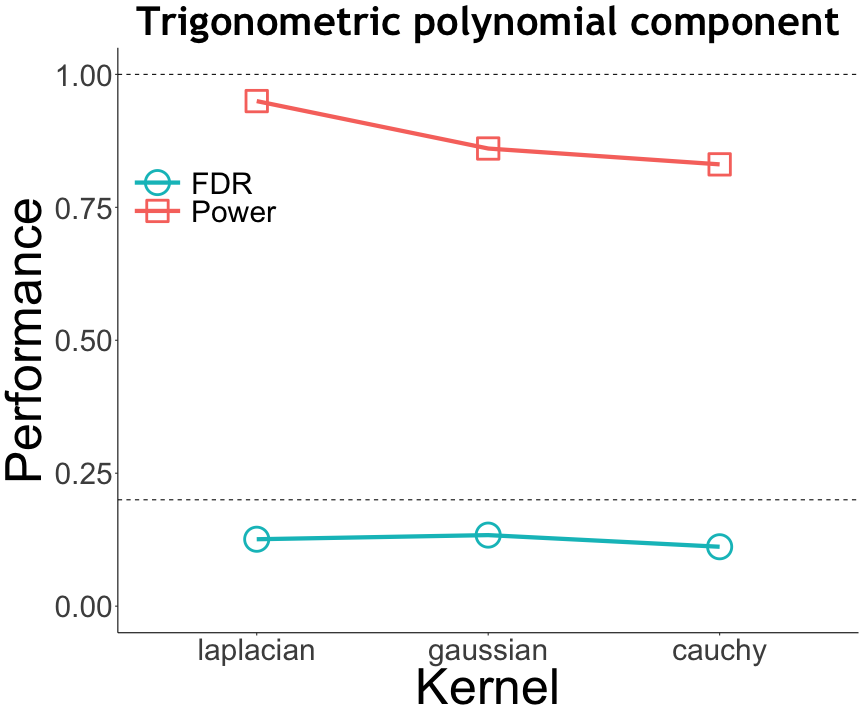
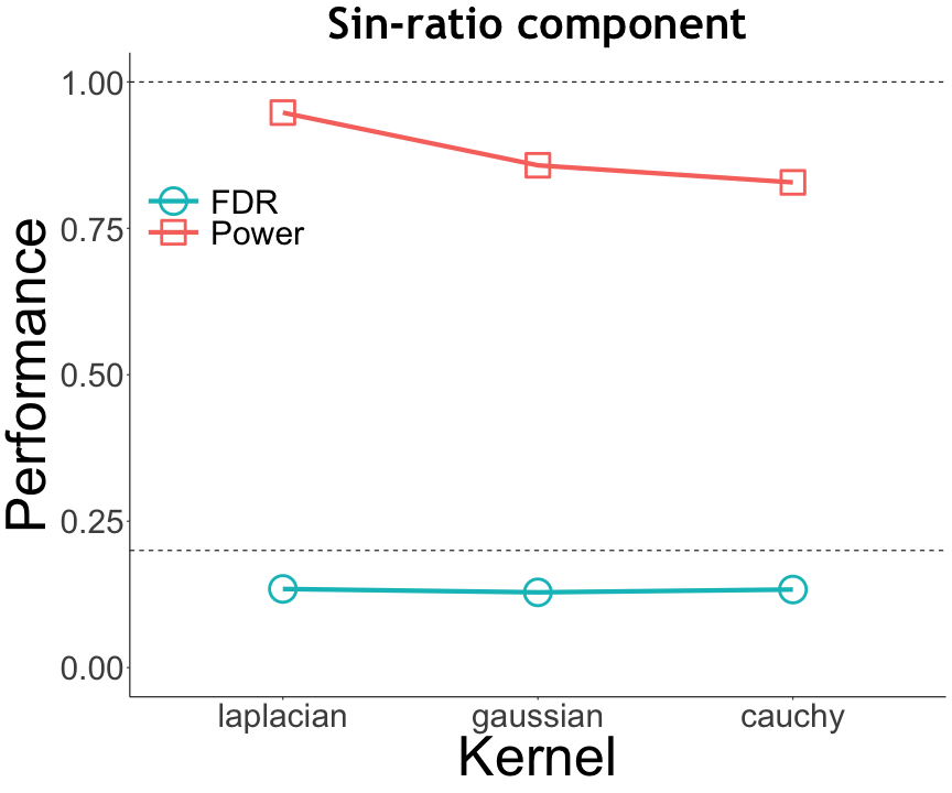
Refer to caption
Refer to caption
Figure 6: Sensitivity analysis to the choice of kernel.

B.2 Sensitivity analysis to the tuning parameters

We next carry out a sensitivity analysis of the kernel knockoffs method with respect to the tuning parameters. Specifically, we tune the number of random features r𝑟r and the regularization parameter τ𝜏\tau following the criteria in Section 3.5, and we study here the sensitivity to the choice of the number of subsampling replications L𝐿L, and the subsampling sample size nssubscript𝑛𝑠n_{s}.

L𝐿L nssubscript𝑛𝑠n_{s}
Refer to caption Refer to caption
Figure 7: Sensitivity analysis to the choice of the tuning parameters.

For L𝐿L, we adopt the same simulation setup as in Section B.1 with the trigonometric polynomial function (15). We vary L={100,200,300,400,500}𝐿100200300400500L=\{100,200,300,400,500\}, and set ns=n/2subscript𝑛𝑠𝑛2n_{s}=\lfloor n/2\rfloor. Figure 7 (left panel) reports the FDR and power with the varying L𝐿L based on 200 data replications. It is seen that the method performs slightly better with a larger L𝐿L, but the performance is relatively robust. Since a larger L𝐿L implies a heavier computation, we set L=300𝐿300L=300 for all other simulations.

For nssubscript𝑛𝑠n_{s}, we adopt the same simulation setup as in Section B.1 with the trigonometric polynomial function (15). We vary the fraction ns/n={0.1,0.3,0.5,0.7,0.9,1}subscript𝑛𝑠𝑛0.10.30.50.70.91n_{s}/n=\{0.1,0.3,0.5,0.7,0.9,1\} and set L=300𝐿300L=300. Figure 7 (right panel) reports the FDR and power with the varying fraction based on 200 data replications. It is seen that the FDR is consistently below the nominal level, and the power becomes stable once nssubscript𝑛𝑠n_{s} is no smaller than n/2𝑛2\lfloor n/2\rfloor. We set ns=n/2subscript𝑛𝑠𝑛2n_{s}=\lfloor n/2\rfloor for all other simulations.

B.3 Predictor correlation

In the simulations so far, we have considered to simulate the predictors from a multivariate normal distribution with mean zero and covariance Σij=ρ|ij|subscriptΣ𝑖𝑗superscript𝜌𝑖𝑗\Sigma_{ij}=\rho^{|i-j|}, where we fix ρ=0.3𝜌0.3\rho=0.3. Next, we consider more correlation values for ρ𝜌\rho. Specifically, we adopt the same simulation setup as in Section B.1 with the trigonometric polynomial function (15). We vary ρ={0.3,0.4,0.5,0.6,0.7,0.8}𝜌0.30.40.50.60.70.8\rho=\{0.3,0.4,0.5,0.6,0.7,0.8\}. Figure 8 reports the FDR and power based on 200 data replications. It is seen that our method maintains the FDR control and a good power across different values of the correlation ρ𝜌\rho.

Refer to caption
Refer to caption
Figure 8: Empirical performance and comparison in terms of FDR and power with the varying predictor correlation ρ𝜌\rho. The same four methods as in Figure 2 are compared.

B.4 Sparsity level

In the power analysis in Section 4.2, we require that the number of nonzero component functions |𝒮|𝒮|{\mathcal{S}}| to be bounded in Assumption 2. Next, we carry out a numerical experiment and show empirically that our method still works reasonably well when the number of nonzero components |𝒮|𝒮|{\mathcal{S}}| increases along with the sample size n𝑛n.

Specifically, we adopt the same simulation setup as in Section B.1 with the trigonometric polynomial function (15). We vary (|𝒮|,n)={(10,900),(20,1800),(30,2700),(40,3600)}𝒮𝑛10900201800302700403600(|{\mathcal{S}}|,n)=\{(10,900),(20,1800),(30,2700),(40,3600)\}. Figure 9 reports the FDR and power based on 200 data replications. It is seen that our method maintains a reasonably good performance, and still outperforms all the alternative solutions when |𝒮|𝒮|{\mathcal{S}}| increases along with n𝑛n.

Refer to caption
Refer to caption
Figure 9: Empirical performance and comparison in terms of FDR and power with the varying number of nonzero component functions |𝒮|𝒮|{\mathcal{S}}|. The same four methods as in Figure 2 are compared.

B.5 Computation parallelization

We note that the computation of our method can be easily parallelized. This is because it requires no information sharing across different subsamples, and thus Steps 2 to 4 in Algorithm 1 can be parallelized. We next carry out a numerical experiment to further investigate the computational acceleration by parallelization.
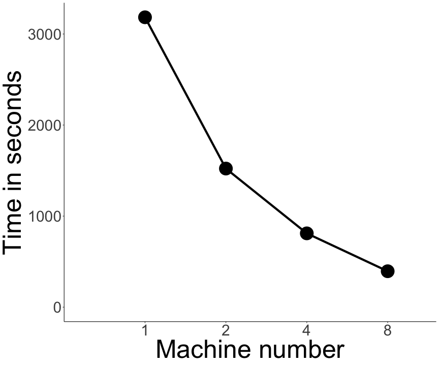
Refer to caption
Figure 10: Average computation time, in seconds, of Algorithm 1 with the varying number of parallel machines. The x-axis is rescaled by base-2 logarithm.

Specifically, we adopt the same simulation setup as in Section B.1 with the trigonometric polynomial function (15). We parallelize the L𝐿L subsamples to a total of M𝑀M machines using the R package foreach. Each machine independently runs Steps 2 to 4 of Algorithm 1 on the allocated subsamples, then the results are aggregated from all machines to perform Steps 5 to 6 of Algorithm 1. We use the c4.4xlarge instance in Amazon Web Services (AWS). We vary the number of machines M={1,2,4,8}𝑀1248M=\{1,2,4,8\}. Figure 10 reports the average computation time, in seconds, of running the entire Algorithm 1 for one data replication, while the results are averaged over 200 data replications. It is seen that the computation time reduces significantly as the number of machines increases.

B.6 Alternative importance scores

Finally, we investigate some alternative importance scores studied in Candès et al. (2018), and compare them with our importance score in the kernel knockoffs method that is built on the selection probability of the variables and their knockoffs across multiple subsamples.

Specifically, let δjsubscript𝛿𝑗\delta_{j} and δ~jsubscript~𝛿𝑗\widetilde{\delta}_{j} denote some importance measure of variable Xjsubscript𝑋𝑗X_{j} and the knockoff variable X~jsubscript~𝑋𝑗\widetilde{X}_{j}, respectively. Candès et al. (2018, Section 4.1) considered three importance scores:

Coefficient difference (CD)::Coefficient difference (CD)absent\displaystyle\textrm{Coefficient difference (CD)}: |δj||δ~j|,subscript𝛿𝑗subscript~𝛿𝑗\displaystyle|\delta_{j}|-|\widetilde{\delta}_{j}|,
Log-coefficient difference (log-CD)::Log-coefficient difference (log-CD)absent\displaystyle\textrm{Log-coefficient difference (log-CD)}: log(|δj|)log(|δ~j|),subscript𝛿𝑗subscript~𝛿𝑗\displaystyle\log(|\delta_{j}|)-\log(|\widetilde{\delta}_{j}|),
Signed max (SM)::Signed max (SM)absent\displaystyle\textrm{Signed max (SM)}: sign(|δj||δ~j|)max{|δj|,|δ~j|},signsubscript𝛿𝑗subscript~𝛿𝑗subscript𝛿𝑗subscript~𝛿𝑗\displaystyle\textrm{sign}(|\delta_{j}|-|\widetilde{\delta}_{j}|)\max\left\{|\delta_{j}|,|\widetilde{\delta}_{j}|\right\},

We adopt the same simulation example as in Section 5.2 with the trigonometric polynomial function (15) and the varying signal strength θ𝜃\theta. Following Candès et al. (2018), we choose the Euclidean norm of the estimated component function as δjsubscript𝛿𝑗\delta_{j} for the coefficient difference score, whereas we choose the penalty value at which the variable enters the model as δjsubscript𝛿𝑗\delta_{j} for the log-coefficient difference score and the signed max score. Moreover, since Candès et al. (2018) did not use subsampling for stability, all these scores are computed based on a single random feature expansion. Figure 11 reports the FDR and power of the selection results based on these three importance scores as well as our kernel knockoff score for 200200200 data replications. It is clearly seen that our importance score performs much better than those alternative scores. In particular, the coefficient difference score and the log-coefficient difference score can not control the FDR below the nominal level. The signed max score can control the FDR, but its power is much lower than the power of our kernel knockoffs method.
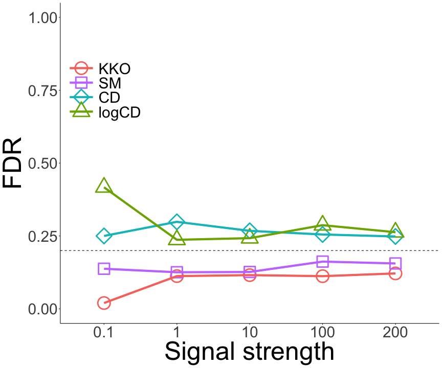
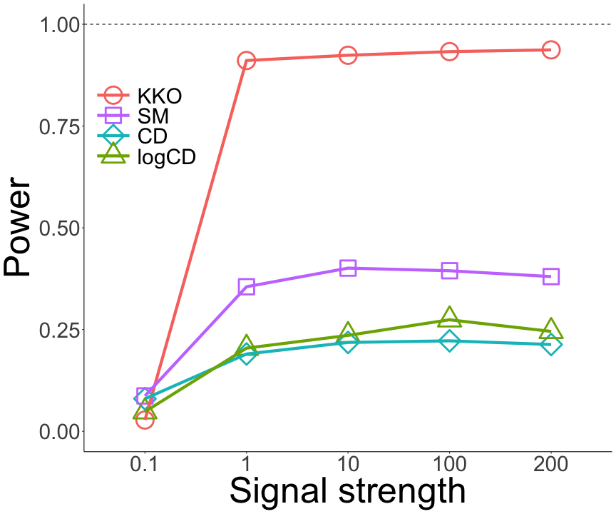
Refer to caption
Refer to caption
Figure 11: Empirical performance and comparison in terms of FDR and power for different importance score functions: our kernel knockoff score (KKO), the coefficient difference score (CD), the log-coefficient difference score (log-CD), and the signed max score (SM).