Dynamic Dual Sampling Module for Fine-Grained Semantic Segmentation
Abstract
Representation of semantic context and local details is the essential issue for building modern semantic segmentation models. However, the interrelationship between semantic context and local details is not well explored in previous works. In this paper, we propose a Dynamic Dual Sampling Module (DDSM) to conduct dynamic affinity modeling and propagate semantic context to local details, which yields a more discriminative representation. Specifically, a dynamic sampling strategy is used to sparsely sample representative pixels and channels in the higher layer, forming adaptive compact support for each pixel and channel in the lower layer. The sampled features with high semantics are aggregated according to the affinities and then propagated to detailed lower-layer features, leading to a fine-grained segmentation result with well-preserved boundaries. Experiment results on both Cityscapes and Camvid datasets validate the effectiveness and efficiency of the proposed approach. Code and models will be available at x3https://github.com/Fantasticarl/DDSM.
Index Terms— Dynamic Sampling, Affinity Modeling
1 Introduction
Semantic segmentation, which entails assigning a label to each pixel of an image, is useful in a growing number of applications, including augmented reality, surveillance, and autonomous driving. With the development of deep FCN networks [1, 2, 3], the related works mainly focus on two aspects: global context modeling [2, 4] and local details modeling [5]. The former models the long-range dependencies among pixels on the higher level of the network by overcoming the limited receptive field of the convolution network. The latter imports extra components such as lower-level features [6] or includes edge supervision [7] for finer and detailed results. The feature pyramids encode different scaled features where the higher layers contain coarse semantics while the lower layers represent fine details [8, 9]. However, the interrelationship between semantic context and local details is not well explored. In this paper, we focus on exploring the interrelationship between two different layers. Since the semantic gaps [10], our solution enhances lower-layer features based on its affinity with the higher layer instead of directly adding features in FPN [8], successfully propagating the semantic context to local details via dynamic sampling of representative pixels and channels in higher layers.
(a)
(c)
(e)
(b)
(d)
(f)
It is noted that the existing affinity modeling methods, including self-attention based [12] or graph-based [13] models, require expensive pixel-wised computation across the whole image. For instance, FPT [14] uses a transformer to model the adjacent features’ affinity, leading to immense resource cost. There is a rather high redundancy since the natural image meets the piece-wise smoothness constraint that the pixels within the same segment share certain visual characteristics. Accordingly, inspired by dynamic graph modeling [15, 16] and deformable convolutions [17, 18], we propose a dynamic affinity modeling method to avoid redundancy and achieve efficient feature propagation. Rather than using full pixels, we sample representative pixels to form adaptive compact support. Furthermore, we propose a dynamic sampler based on DCNv2 [18] instead of sampling fixed neighborhood pixels to fit the orientation distribution of image structures. Moreover, the channel encodes corresponding class-specific information, and several works [3] have shown the advantages of considering spatial and channel simultaneously to enhance class-aware information in feature representation. Hence, we also apply the dynamic sampler in feature channels and conduct channel-wise dynamic affinity modeling. After obtaining the sampled pixels/channels, we calculate both spatial and channel-wise affinities for each pixel/channel in the lower-layer. Finally, relevant semantics is aggregated according to the affinities and propagated to detailed lower-layer features.
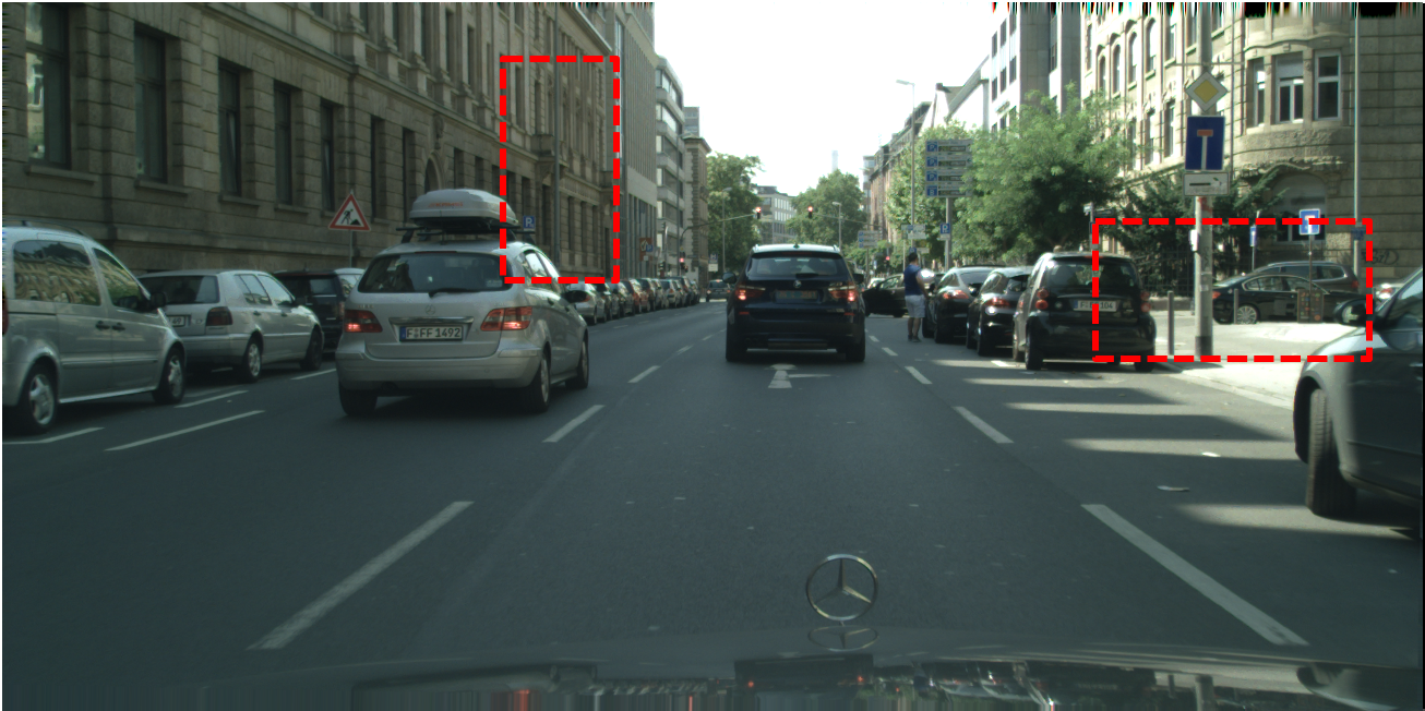
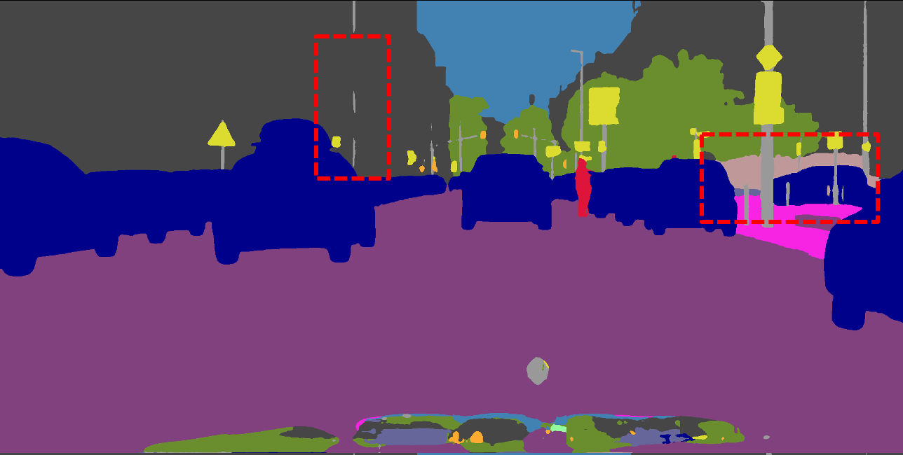
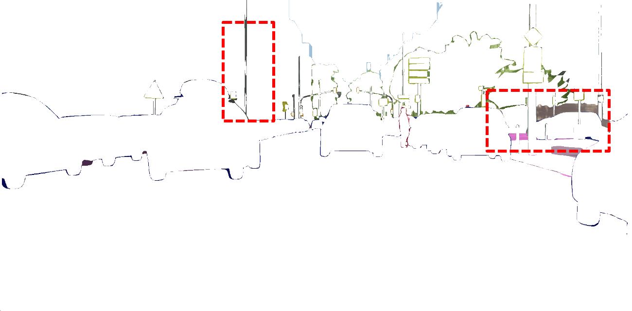
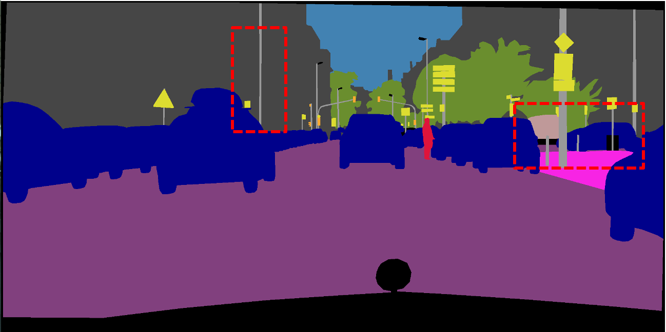
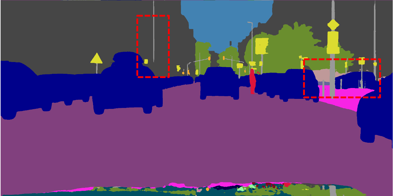
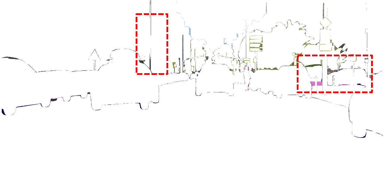
In summary, we propose a Dynamic Dual Sampling Module(DDSM), which contains spatial-wise and channel-wise dynamic affinity modeling. The representation of the pixels /channels in the lower layer is enhanced by some dynamically sampled pixels/channels from the higher layer. We validate DDSM’s effectiveness on two typical networks, UPerNet [11] and Deeplabv3+ [6]. Notably, our method could provide fine-grained segmentation results with well-preserved boundaries. Fig. 1 shows the error map refined by DDSM based on UPerNet [11]. After inserting DDSM into UPerNet [11], it achieves competitive results on Cityscapes [19] and Camvid [20]. In particular, DDSM outperforms DAnet [3] with only 30% computation during the inference.
2 Method
In this section, we first describe our dynamic sampler, which is inspired by DCNv2 [18]. Then, we give a detailed introduction of our proposed Dynamic dual sampling module, which dynamically samples pixels and channels simultaneously. Finally, we deploy our proposed module into two frameworks.
2.1 Dynamic Sampler
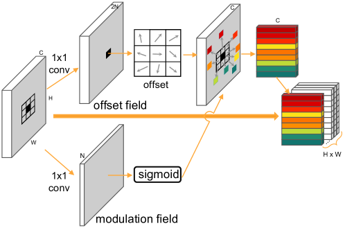
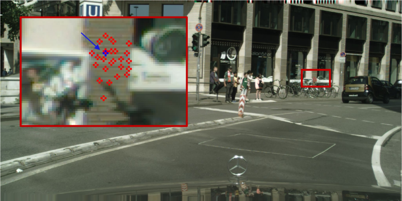
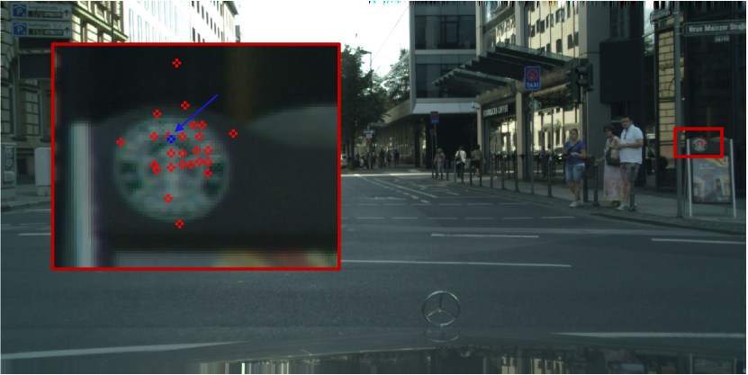
Given the input features with dimension , the sampler dynamically samples pixels from for each position , as Fig. 2 shows. Specifically, a regular grid is defined to get an initial sampling area of . Then, we use a convolution layer instead of in DCN [17] to learn an offset for each position in the grid , and then an offset map with dimension of is obtained, in which 2D offsets are learned. With the offset map, we use bilinear interpolation to compute the sampled features of each sampled position . To learn the offset map more flexibly and further boost the performance, a learnable scalar is added following the work of DCNv2 [18]. Given the dynamic sampler , the sampled features can be formulated as Eq.1:
| (1) |
The output () gives the features at positions sampled from for each position in the feature map.
2.2 Dynamic Dual Sampling Module(DDSM)
(a) Spatial-wise dynamic affinity modeling
(b) Channel-wise dynamic affinity modeling
The Dynamic Dual Sampling Module consists of two parts, namely spatial-wise dynamic affinity modeling and channel-wise dynamic affinity modeling. The final output is the summation of the output features from both parts.
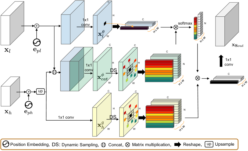
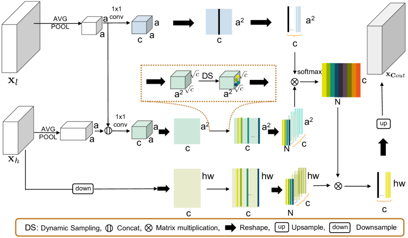
Spatial-wise Dynamic Affinity Modeling: This part dynamically assigns features of pixels sampled from the higher layer for each pixel in the lower layer. As shown in Fig. 3(a), for the low-level features and the high-level features , we first upsample to , same as . Note that position information is crucial in feature fusion. A common method of introducing position information is to summarize features and positional encodings as input [21]. We add learnable positional embeddings [21] , to the features , to disambiguate different spatial positions. Then we concatenate both and into features . Then, we use three convolution layers to do dimension reduction on , , and , forming a new feature set as , , . Similar to the definition in the work [22], , and correspond to Query, Key, and Value function.
The work [22] uses the entire feature map to calculate the affinity map. Nevertheless, we use the dynamic sampler to sample pixels in the Key for each position in the Query to obtain the affinity map. We sample pixels from to form sampled features for each position in . Matrix multiplication is performed between the features of each position in and the transposed sampled features to form the affinity map with softmax normalization. Then, matrix multiplication is performed between the affinity map and sampled features from . The above two processes are executed times to obtain the aggregation result of sampled features, which will be assigned to the low-level features through a summation operation. The spatial-wise dynamic affinity modeling is formulated as Eq.2,
| (2) |
where is the augmented feature, is a position in and is Softmax. Fig. 3(a) gives the detailed pipline.
Channel-wise Dynamic Affinity Modeling: The channel-wise dynamic affinity modeling is built to explore interdependencies along channels since the channel encodes class-specific information. Different from previous works [3, 23], our module dynamically samples the channels of high-level features and aggregates them according to affinity to enhance low-level features. The input and are both average pooled to to reduce the spatial resolution. and is concatenated and then reshaped to to perform channel-wise dynamic sampling. As Fig. 3(b) shows, in order to reuse the dynamic sampler , we reshape the features with dimension into (we set channel as a square number 64 in this work), and then reshape back to for affinity calculation after the sampling of channels. For each channel in the pooled low-level feature, the affinity map is calculated with the corresponding sampled channels. Finally, the high-level features are also dynamically sampled in the channel dimension and propagated to the corresponding channel of the low-level features according to the affinity map. Note that we downsample to to reduce computation here. The whole process can be formulated as Eq. 3:
| (3) |
where is the channel in low-level features, , ), , and are the pooled low-level and high-level features, is the downsampled high-level features, means Softmax, ,, are implemented with convolution layers.
Plugin into Two Architectures: Our proposed DDSM is end-to-end trainable, and it can dynamically propagate rich semantic information between adjacent features. We use DDSM in UPerNet [11], which contains FPN[24] with Pyramid Pooling Module(PPM)[2], and Deeplabv3+[6]. In UPerNet [11], we replace the upsample module with the proposed DDSM. Let be the output of each stage in encoder, e.g. ResNet [25]. The enhanced higher-level features and the corresponding are passed into DDSM to form their enhanced bottom level features . For Deeplabv3+ [6], we insert one DDSM module which dynamically assigns the output of ASPP to the low-level to form for final segmentation.
3 Experiment
(a) Input
(b)
(b)
(d)
(e)
(f)
In order to verify the effectiveness of our proposed DDSM, we conduct thorough experiments on Cityscapes[19] and CamVid[20]. The mean Intersection over Union (mIoU) is adopted as the evaluation metric in all experiments, and F-Score[26] is used to measure the boundary performance.
Implementation details: Our method is implemented using the Pytorch framework. For all our experiments, an SGD is used as the optimizer, momentum and weight decay are set to 0.9 and 5e-4, respectively. The learning rate is set as 0.01 and is decayed by multiplying . For data augmentation in training, we employ a random horizontal flip, a random resize with scale range [0.75,2], and then a random crop of for Cityscapes ( for Camvid).
Ablation study:
To verify the effectiveness of each component of our method, we conduct multiple sets of experiments on Cityscapes, including whether to use DCN [17], spatial-wise and channel-wise dynamic affinity modeling or not. We insert two DDSMs into the second and third stages of UPerNet [11]. The number of sampled spatial positions and channels are both set to 9. As shown in Table 1, based on UPerNet [11], both spatial and channel-wise dynamic modules will bring more benefits than DCN [17]. A mix of both modules improves the performance by 1.26%. Simultaneously, to verify the applicability of DDSM in different frameworks, we insert one DDSM in Deeplabv3+ [6]. Table 1(right) also shows the performance improvement of DDSM
on Deeplabv3+.
| Ablation on UPerNet [11] | Ablation on Deeplabv3+ [6] | ||||
|---|---|---|---|---|---|
| Method | mIoU(%) | (%) | Method | mIoU(%) | (%) |
| UPerNet [11] | 78.39 | - | Deeplabv3+ [6] | 77.76 | - |
| UPerNet+DCN [17] | 78.51 | 0.12 | Deeplabv3++DCN [17] | 78.09 | 0.33 |
| UPerNet+S | 79.25 | 0.86 | Deeplabv3++S | 78.34 | 0.58 |
| UPerNet+C | 78.99 | 0.60 | Deeplabv3++C | 78.22 | 0.46 |
| UPerNet+S+C | 79.65 | 1.26 | Deeplabv3++S+C | 78.57 | 0.81 |
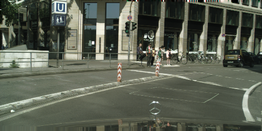
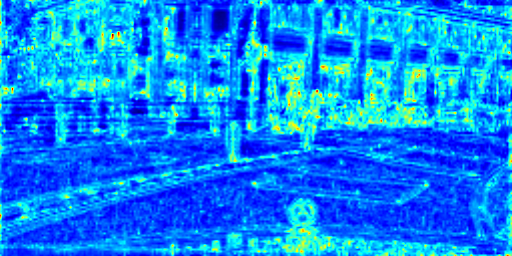
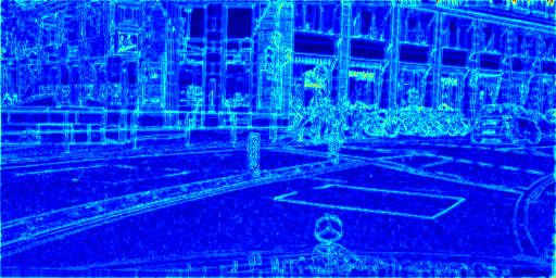
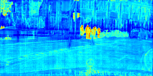
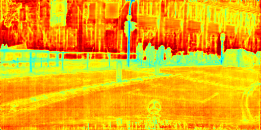
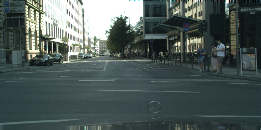
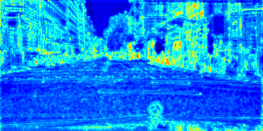
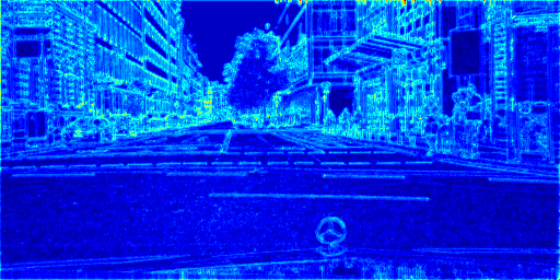
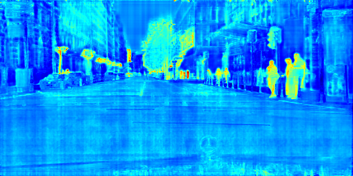
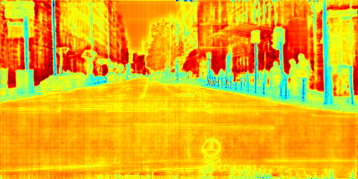
Analysis of Boundary F-Score and Visualizations: To show the advantages of our model at the boundaries, we adopt the boundary F-Score [26] to measure the segmentation accuracy at the boundaries. Table 2 shows the boundary F-Score under different thresholds. Our model is entirely ahead of the baseline, proving its advantages at the boundaries. We also visualize the input and output features of DDSM, as shown in Fig. 4. All feature maps are averaged along channels for display. The visualizations show that DDSM can dynamically propagate high-level semantic information to detailed low-level features from spatial and channel domain.
| Threshhold | 3px | 5px | 9px | 12px | mean |
|---|---|---|---|---|---|
| UPerNet [11] | 66.4 | 76.3 | 80.1 | 81.5 | 76.1 |
| Ours | 69.3 | 78.9 | 82.3 | 83.6 | 78.5 |
Comparison with previous work: The mIoU of our results on the Cityscapes test set reaches 81.7%, which performs favorably against state-of-the-art segmentation methods. Meantime, our method has shown advantages in terms of computational consumption, which is only about 30% of DAnet’s [3], as Table 3 shows. We sample 25 pixels and 9 channels here to obtain further performance improvement according to the ablation study. We insert three DDSMs in UPerNet [11] to form , , . Multi-scale testing is conducted following CCNet [27]. Table 3 also shows the advantages of our method over the Non-Local based methods.
| Model | Reference | Backbone | mIoU(%) | #Params | #GFLOPs |
|---|---|---|---|---|---|
| DFN [28] | CVPR2018 | ResNet-101 | 79.3 | 90.7M | 1121.0 |
| PSANet [29] | ECCV2018 | ResNet-101 | 80.1 | 85.6M | 1182.6 |
| DenseASPP [30] | CVPR2018 | DenseNet-161 | 80.6 | 35.7M | 632.9 |
| ANNet [31] | ICCV2019 | ResNet-101 | 81.3 | 63.0M | 1089.8 |
| CPNet [32] | CVPR2020 | ResNet-101 | 81.3 | - | - |
| CCNet [27] | ICCV2019 | ResNet-101 | 81.4 | 66.5M | 1153.9 |
| RGNet [16] | ECCV2020 | ResNet-101 | 81.5 | - | - |
| DANet [3] | CVPR2019 | ResNet-101 | 81.5 | 66.6M | 1298.8 |
| Ours | - | ResNet-101 | 81.7 | 51.8M | 367.5 |
Experiments on CamVid: To further verify the effectiveness of DDSM, we also conduct experiments on the CamVid dataset. Table 4 shows our results on CamVid. Our model without Cityscapes pre-training outperforms the others. After pre-training, the mIoU performance is improved to 80.6%.
4 Conclusion
We propose an end-to-end trainable Dynamic Dual Sampling Module for both spatial-wise dynamic affinity modeling and channel-wise dynamic affinity modeling between two different features. Thus lower layer features are dynamically enhanced by the features of representative pixels and channels from the higher layer simultaneously. Through lots of experiments, our proposed DDSM is verified to be effective on different networks. Our model achieves advanced performance on the Cityscapes and Camvid datasets while significantly reducing computational consumption.
References
- [1] Jonathan Long, Evan Shelhamer, and Trevor Darrell, “Fully convolutional networks for semantic segmentation,” in CVPR, 2015.
- [2] Hengshuang Zhao, Jianping Shi, Xiaojuan Qi, Xiaogang Wang, and Jiaya Jia, “Pyramid scene parsing network,” in CVPR, 2017.
- [3] Jun Fu, Jing Liu, Haijie Tian, Zhiwei Fang, and Hanqing Lu, “Dual attention network for scene segmentation,” arXiv preprint arXiv:1809.02983, 2018.
- [4] Liang-Chieh Chen, George Papandreou, Florian Schroff, and Hartwig Adam, “Rethinking atrous convolution for semantic image segmentation,” arXiv preprint arXiv:1706.05587, 2017.
- [5] Xiangtai Li, Zhao Houlong, Han Lei, Tong Yunhai, and Yang Kuiyuan, “Gff: Gated fully fusion for semantic segmentation,” in AAAI, 2020.
- [6] Liang-Chieh Chen, Yukun Zhu, George Papandreou, Florian Schroff, and Hartwig Adam, “Encoder-decoder with atrous separable convolution for semantic image segmentation,” in ECCV, 2018.
- [7] Xiangtai Li, Xia Li, Li Zhang, Cheng Guangliang, Jianping Shi, Zhouchen Lin, Yunhai Tong, and Shaohua Tan, “Improving semantic segmentation via decoupled body and edge supervision,” in ECCV, 2020.
- [8] Tsung-Yi Lin, Piotr Dollár, Ross B. Girshick, Kaiming He, Bharath Hariharan, and Serge J. Belongie, “Feature pyramid networks for object detection,” in CVPR, 2017.
- [9] Xiangtai Li, Ansheng You, Zhen Zhu, Houlong Zhao, Maoke Yang, Kuiyuan Yang, Shaohua Tan, and Yunhai Tong, “Semantic flow for fast and accurate scene parsing,” in ECCV. Springer, 2020, pp. 775–793.
- [10] Henghui Ding, Xudong Jiang, Bing Shuai, Ai Qun Liu, and Gang Wang, “Context contrasted feature and gated multi-scale aggregation for scene segmentation,” in CVPR, June 2018.
- [11] Tete Xiao, Yingcheng Liu, Bolei Zhou, Yuning Jiang, and Jian Sun, “Unified perceptual parsing for scene understanding,” in ECCV, 2018.
- [12] Yunpeng Chen, Yannis Kalantidis, Jianshu Li, Shuicheng Yan, and Jiashi Feng, “A^2-nets: Double attention networks,” in NeurIPS. 2018.
- [13] Yin Li and Abhinav Gupta, “Beyond grids: Learning graph representations for visual recognition,” in NeurIPS. 2018.
- [14] Dong Zhang, Hanwang Zhang, Jinhui Tang, Meng Wang, Xiansheng Hua, and Qianru Sun, “Feature pyramid transformer,” in ECCV. Springer, 2020, pp. 323–339.
- [15] Li Zhang, Dan Xu, Anurag Arnab, and Philip H.S. Torr, “Dynamic graph message passing networks,” in CVPR, June 2020.
- [16] Changqian Yu, Yifan Liu, Changxin Gao, Chunhua Shen, and Nong Sang, “Representative graph neural network,” in ECCV, 2020.
- [17] Jifeng Dai, Haozhi Qi, Yuwen Xiong, Yi Li, Guodong Zhang, Han Hu, and Yichen Wei, “Deformable convolutional networks,” in ICCV, 2017.
- [18] Xizhou Zhu, Han Hu, Stephen Lin, and Jifeng Dai, “Deformable convnets v2: More deformable, better results,” in CVPR, 2019, pp. 9308–9316.
- [19] Marius Cordts, Mohamed Omran, Sebastian Ramos, Timo Rehfeld, Markus Enzweiler, Rodrigo Benenson, Uwe Franke, Stefan Roth, and Bernt Schiele, “The cityscapes dataset for semantic urban scene understanding,” in CVPR, 2016.
- [20] Gabriel J Brostow, Julien Fauqueur, and Roberto Cipolla, “Semantic object classes in video: A high-definition ground truth database,” Pattern Recognition Letters, vol. 30, no. 2, pp. 88–97, 2009.
- [21] Nicolas Carion, Francisco Massa, Gabriel Synnaeve, Nicolas Usunier, Alexander Kirillov, and Sergey Zagoruyko, “End-to-end object detection with transformers,” in ECCV. Springer, 2020, pp. 213–229.
- [22] Ashish Vaswani, Noam Shazeer, Niki Parmar, Jakob Uszkoreit, Llion Jones, Aidan N Gomez, Lukasz Kaiser, and Illia Polosukhin, “Attention is all you need,” in NeurIPS, 2017.
- [23] Jie Hu, Li Shen, and Gang Sun, “Squeeze-and-excitation networks,” in CVPR, 2018.
- [24] Alexander Kirillov, Kaiming He, Ross B. Girshick, and Piotr Dollár, “A unified architecture for instance and semantic segmentation,” 2017.
- [25] Kaiming He, Xiangyu Zhang, Shaoqing Ren, and Jian Sun, “Deep residual learning for image recognition,” in CVPR, 2016.
- [26] Federico Perazzi, Jordi Pont-Tuset, Brian McWilliams, Luc Van Gool, Markus Gross, and Alexander Sorkine-Hornung, “A benchmark dataset and evaluation methodology for video object segmentation,” in CVPR, 2016, pp. 724–732.
- [27] Zilong Huang, Xinggang Wang, Lichao Huang, Chang Huang, Yunchao Wei, and Wenyu Liu, “Ccnet: Criss-cross attention for semantic segmentation,” in ICCV, 2019, pp. 603–612.
- [28] Changqian Yu, Jingbo Wang, Chao Peng, Changxin Gao, Gang Yu, and Nong Sang, “Learning a discriminative feature network for semantic segmentation,” in CVPR, 2018.
- [29] Hengshuang Zhao, Yi Zhang, Shu Liu, Jianping Shi, Chen Change Loy, Dahua Lin, and Jiaya Jia, “Psanet: Point-wise spatial attention network for scene parsing,” in ECCV, 2018.
- [30] Maoke Yang, Kun Yu, Chi Zhang, Zhiwei Li, and Kuiyuan Yang, “Denseaspp for semantic segmentation in street scenes,” in CVPR, 2018.
- [31] Zhen Zhu, Mengde Xu, Song Bai, Tengteng Huang, and Xiang Bai, “Asymmetric non-local neural networks for semantic segmentation,” in ICCV, 2019, pp. 593–602.
- [32] Changqian Yu, Jingbo Wang, Changxin Gao, Gang Yu, Chunhua Shen, and Nong Sang, “Context prior for scene segmentation,” in CVPR, 2020, pp. 12416–12425.
- [33] Piotr Bilinski and Victor Prisacariu, “Dense decoder shortcut connections for single-pass semantic segmentation,” in CVPR, 2018.
- [34] Siddhartha Chandra, Camille Couprie, and Iasonas Kokkinos, “Deep spatio-temporal random fields for efficient video segmentation,” in CVPR, 2018, pp. 8915–8924.