Unsupervised Scale-consistent Depth Learning from Video

Abstract

We propose a monocular depth estimator SC-Depth, which requires only unlabelled videos for training and enables the scale-consistent prediction at inference time. Our contributions include: (i) we propose a geometry consistency loss, which penalizes the inconsistency of predicted depths between adjacent views; (ii) we propose a self-discovered mask to automatically localize moving objects that violate the underlying static scene assumption and cause noisy signals during training; (iii) we demonstrate the efficacy of each component with a detailed ablation study and show high-quality depth estimation results in both KITTI and NYUv2 datasets. Moreover, thanks to the capability of scale-consistent prediction, we show that our monocular-trained deep networks are readily integrated into ORB-SLAM2 system for more robust and accurate tracking. The proposed hybrid Pseudo-RGBD SLAM shows compelling results in KITTI, and it generalizes well to the KAIST dataset without additional training. Finally, we provide several demos for qualitative evaluation. The source code is released on GitHub.

1 Introduction

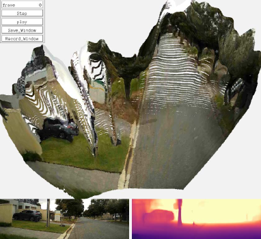
(a) Predicted depth and textured point cloud

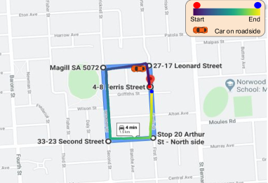
(b) Qualitative evaluation of estimated trajectory

Figure 1: Generalization on our self-captured video. The data is collected in Adelaide, an Australia city. Our depth and pose networks are trained on KITTI without additional finetuning. The scene is so challenging that ORB-SLAM2 Mur-Artal & Tardós (2017) failed to initialize or quickly lost tracking after initialization, while our Pseudo-RGBD SLAM system can provide an accurate trajectory, which is consistent with the Google Map. See more details in Sec. 5.4.

The CNN-based monocular depth estimation Eigen et al. (2014) has shown significant promise for many Computer Vision tasks. The supervised methods Fu et al. (2018); Yin et al. (2019) achieve high performance, while they require expensive range sensors to capture the ground-truth data for training. To this end, recent work explores unsupervised learning for monocular depth estimation, which either uses the calibrated stereo pairs Garg et al. (2016); Godard et al. (2017) or unlabelled videos Zhou et al. (2017); Yin & Shi (2018) for training. In these frameworks, the color consistency between multiple views serves as the main supervision signal. Since they do not require ground truth labels, and particularly the recent method  Gordon et al. (2019) showing unsupervised depth estimation can work with the unknown camera intrinsics, these methods attract a lot of interest in the Computer Vision community. In this paper, we are interested in the video-based unsupervised learning framework because it has a minimum requirement for training data.

Compared with stereo-based learning, video-based learning Zhou et al. (2017) is often more challenging due to the unknown camera motion. More importantly, due to scale ambiguity, a natural issue in monocular vision, the predicted depth by the latter has an unknown scaling to the real world. This is the so-called relative depth, as opposed to the metric depth in the previous setting. The relative depth is also widely used, e.g., ORB-SLAM Mur-Artal et al. (2015) and COLMAP Schonberger & Frahm (2016) both generate results up to an unknown scale. However, one critical issue that we identify in video-based learning is that methods may generate scale-inconsistent predictions over different frames since they suffer from a per-frame scale ambiguity. This does not impact the single-image based tasks, while it is critical for video-based applications, e.g., inconsistent depths cannot be used for camera tracking in the Visual SLAM system—See Fig. 9.

In this paper, we propose an improved unsupervised learning framework for higher depth accuracy and consistency. First, we propose a geometry consistency loss ($L_{G}$) to encourage networks to predict scale-consistent depths. It explicitly penalizes the pixel-wise inconsistency of predicted depths between adjacent frames during training. It enables more effective learning and allows for more consistent predictions at inference time—See Tab. 6. Second, we propose a self-discovered mask ($M_{s}$) for handling moving objects during training, which violates the underlying static scene assumption. It improves the performance significantly (See Tab. 2) and does not require additional overhead since the proposed mask is simply derived from $L_{G}$.

To show the benefits from scale-consistent depth prediction and demonstrate our contribution for downstream tasks, we integrate our trained networks into the ORB-SLAM2 Mur-Artal & Tardós (2017) system for more accurate and robust tracking. The proposed hybrid Pseudo-RGBD SLAM system has distinct advantages over traditional monocular systems, including a) it starts tracking at any frame without latency; b) it enables more robust and accurate tracking with the help of predicted depths; and c) it allows for dense 3D reconstruction—See Fig. 12. We report comprehensive quantitative results and provide several demos in Sec. 5.4 for qualitative evaluation. An example is shown in Fig. 1, where we visualize the depth, point cloud, and camera trajectory generated by our method on a real-world driving video.

Our preliminary version was presented in NeurIPS 2019 Bian et al. (2019b), where we propose an unsupervised learning framework for scale-consistent depth and pose estimation. In this paper, we i) add more technical details of our proposed method; ii) make a more clear explanation of our contribution and distinguish our method from existing methods; iii) improve our learning framework by changing network architectures and integrating effective components from related work; iv) conduct a more comprehensive evaluation and show the potential of our method to Visual SLAM.

2 Related work

Single-view depth estimation.

The depth estimation problem was mainly solved by using traditional geometry based methods Geiger et al. (2011); Schönberger et al. (2016) before deep learning based methods emerged. They rely on correspondences search Lowe (2004); Bian et al. (2019a), model fitting Zhang (1998); Bian et al. (2019c), and multi-view triangulation Hartley & Zisserman (2003). Therefore, at least two different views of the scene are required as input for computing the depth. In contrast, recent deep learning based methods leverage the expressive power of convolutional neural networks, and they are able to regress the depth from a single image only. According to the training data, we can categorize learning-based methods into four classes: First, Eigen et al. (2014) use the sensor captured depths (e.g., LiDAR or RGB-D devices) as the ground truth for training. The following work Liu et al. (2016); Fu et al. (2018); Garg et al. (2019); Yin et al. (2019); Huynh et al. (2020) proposes more advanced network architectures or learning objectives to improve the performance. These methods achieve high performance, while it is expensive to capture ground-truth data in many real-world scenes. Second, Xian et al. (2018); Li & Snavely (2018); Li et al. (2019b); Wang et al. (2019); Chen et al. (2019a); Yin et al. (2020) collect stereo images or videos from the web and use off-the-shelf tools (e.g., stereo matching Hirschmuller (2005) or multi-view stereo Schönberger et al. (2016)) to compute dense ground-truth depths. Besides, Ranftl et al. (2020) export perfect depths from the synthetic 3D movies Butler et al. (2012). Although these methods can obtain cheap ground-truth data, there often exists a domain gap between the collected data and the desired scenes. More importantly, the learned scale information is hard to generalize across different scenes so that they often predict the relative depth. This prevents them from predicting consistent depths on a video. Third, Garg et al. (2016) use the calibrated stereo images for training models, where they warp images using the predicted depth with the known camera baseline and use the photometric loss to penalize the warping error. Then Godard et al. (2017) exploit the left-right consistency in image pairs, and Zhan et al. (2018) exploit the temporary consistency in videos. Pilzer et al. (2018) leverage adversarial learning, and Poggi et al. (2020) study the uncertainty of predicted depths. These methods can predict the metric depth, while it requires well-calibrated stereo cameras to collect training data. Fourth, Zhou et al. (2017) train models from unlabelled videos, where they jointly train the depth and pose networks using adjacent frames with photometric loss and differentiable warping Jaderberg et al. (2015). Due to the simplicity and generality,, it attracts a lot of researchers’ interests and inspires a series of works, including Mahjourian et al. (2018); Wang et al. (2018); Yin & Shi (2018); Zou et al. (2018); Ranjan et al. (2019); Godard et al. (2019); Chen et al. (2019b); Gordon et al. (2019); Zhao et al. (2020); Zhou et al. (2019); Klingner et al. (2020); Guizilini et al. (2020a, b). Our method falls into this category, and we target improving the depth accuracy and consistency for advancing downstream video-based tasks.

Scale consistency.

It is an important problem in Visual SLAM Mur-Artal et al. (2015), but to the best of our knowledge, we are the first ones to discuss the scale inconsistency behind unsupervised video-based depth learning. Nevertheless, we find that our proposed geometry consistency loss is technically similar to two previous methods. First, Mahjourian et al. (2018) propose a 3D ICP loss to penalize the misalignment of predicted depths, where they approximate gradients for depth and pose networks independently because the ICP is not differentiable. This ignores second-order effects between depth and pose networks, and hence it limits the performance. By contrast, our geometry consistency loss is naturally differentiable and results in better performance. Second, Zou et al. (2018) propose a depth consistency loss, which enforces corresponding points in two images to have identical depth predictions. This is physically incorrect because the scene depth is view-dependent, i.e., it should be different in different views. We instead synthesize the depth for the second view using the predicted depth in the first view via rigid transformation, and we penalize the difference between predicted depths and synthesized depths in the second view. Not only does our approach improve the depth accuracy, but also it enables scale-consistent depth prediction for advancing video-based applications such Visual SLAM Mur-Artal & Tardós (2017). After the publication of our conference paper, we notice that more recent works pay attention to consistent depth prediction, including Luo et al. (2020); Tiwari et al. (2020); Zhao et al. (2020); Zou et al. (2020).

Moving objects.

As the moving objects violate the underlying static world assumption for learning depths, related work often detects dynamic regions and masks them out when computing the photometric loss. Zhou et al. (2017) predict a mask from a pair of images by using the neural network. However, due to lacking effective supervision signals, the performance is limited. Vijayanarasimhan et al. (2017) learn a moving object mask from synthetic data Menze & Geiger (2015), which is often hard to generalize to real-world scenes. Yin & Shi (2018); Zou et al. (2018); Ranjan et al. (2019); Chen et al. (2019b) additionally train an optical flow network and compare the optical flow with depth-based mapping for detecting moving objects. This is effective, but training an optical flow network is time-consuming due to the complex correlation computation. Casser et al. (2019a); Gordon et al. (2019); Guizilini et al. (2020b); Huynh et al. (2020); Casser et al. (2019b) leverage the semantic information for localizing dynamic objects. They either require the pretrained semantic segmentation network or need the manually labelled class labels for multi-task training. Godard et al. (2019) mask out the moving objects that have the same velocity as the camera, while it cannot handle other object motions. Compared with previous methods, our method does not require semantic inputs and does not require training additional networks. Our proposed mask is analytically derived from the geometry consistency loss, and it is able to handle arbitrary object motions and occlusions. After ours, Li et al. (2020) propose to learn the dense 3D translation field of objects relative to the scene by using the neural network, which is also efficient and effective.

Depth estimation for Visual SLAM.

Traditional methods use either feature matching Geiger et al. (2011); Klein & Murray (2007) or direct image alignment Forster et al. (2014); Engel et al. (2017) for camera tracking and mapping. Recently, Yin et al. (2017) use a supervised depth estimation model to help recover the absolute scale for monocular methods. CNN-SLAM Tateno et al. (2017) uses the depth estimation network within a monocular SLAM system for dense reconstruction. CodeSLAM Bloesch et al. (2018) jointly optimizes the depth and pose via a learned latent code. Although promising results are reported, these methods rely on supervised training, which is not always available in real-world scenarios. UndeepVO Li et al. (2018) and Zhan et al. (2018) train depth and pose networks on the calibrated stereo videos using the photometric loss, and they show that the learned pose network can inference on monocular videos like a visual odometer. CNN-SVO Loo et al. (2019) combines the stereo-learned depth network and SVO Forster et al. (2014) for more accurate trajectory estimation. DVSO Yang et al. (2018a) and D3VO Yang et al. (2020) also train depth models on stereo videos, and they further conduct geometric optimization. Note that all the aforementioned methods do not suffer from the scale ambiguity issue, as opposed to ours, because they can recover the metric depth. In this paper, we show that the monocular-trained model can predict the scale-consistent results, and it can be used for visual odometry. After ours, Zou et al. (2020) propose to model the long-term dependency by using a two-layer convolutional LSTM module, which improves the pose prediction accuracy significantly. However, the pure learning-based methods are easy to overfit, and we believe that combing deep learning and geometry-based methods is a more promising direction. As a result, our hybrid system generalizes well to the previously unseen dataset and to our self-captured videos.

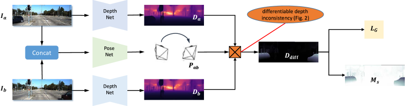
Figure 2: Illustration of the proposed geometry consistency loss and self-discover mask. Given two consecutive frames ($I_{a}$, $I_{b}$), we first estimate their depth maps ($D_{a}$, $D_{b}$) and relative pose ($P_{ab}$) using the network. Then we compute the $D_{\text{diff}}$ (Eqn. 5), i.e., pixel-wise depth inconsistency between $D_{a}$ and $D_{b}$. Finally, we derive our geometric consistency loss $L_{G}$ (Eqn. 6) and self-discovered mask $M_{s}$ (Eqn. 7) from $D_{\textit{diff}}$ to regularize the network training and hanlding dynamics and occlusions (Fig. 4). For clarity, the photometric loss and smoothness loss are not shown in this figure.

Figure 3: Differentiable depth inconsistency computation. This operation takes two depth maps ($D_{a}$, $D_{b}$) and their relative pose ($P_{ab}$) as input and outputs the pixel-wise inconsistency. Firstly, we project $D_{a}$ to 3D space and then to the image plane of $D_{b}$ using $P_{ab}$, obtaining the $D^{a}_{b}$ that stands for the synthesized $D_{b}$. Then, we hope to compute the difference between $D^{a}_{b}$ and $D_{b}$. However, it is not practical because the projection does not religiously lie in the grid of $D_{b}$. Therefore, we obtain the $D^{\prime}_{b}$ by using the differentiable bilinear interpolation Jaderberg et al. (2015). Finally, we compare $D^{a}_{b}$ with $D^{\prime}_{b}$ to obtain the depth inconsistency ($D_{\text{diff}}$). Here, we use the relative loss (Eqn. 5), although other loss functions such as L1 and L2 are also applicable.

3 SC-Depth

3.1 Framework Overview

Our goal is to train depth and pose CNNs from unlabeled videos. Given two adjacent frames ($I_{a}$, $I_{b}$) randomly sampled from a video, their depth maps ($D_{a}$, $D_{b}$) and relative 6-DoF camera pose $P_{ab}$ are first estimated by the depth and pose CNNs, respectively. With the predicted depth and pose, we can synthesize the reference image $I_{a}$ using the source image $I_{b}$ by differentiable warping Jaderberg et al. (2015), which generates $I_{a}^{\prime}$. Then the network is supervised by the photometric loss between the real $I_{a}$ and the synthesized $I_{a}^{\prime}$. To explicitly constrain the depth CNN to predict scale-consistent results on adjacent frames, we propose a geometry consistency loss $L_{G}$. To handle invalid cases such as static frames and dynamic objects, we introduce two masks. First, a self-discovered mask $M_{s}$ (Eqn. 7) is introduced to reason the dynamics and occlusions by checking the depth consistency. Fig. 2 illustrates the proposed loss and mask. Second, we use the auto-mask ($M_{a}$) Godard et al. (2019) to remove stationary points on image pairs where the camera is not moving.

Our objective function is formulated as follows:

$$L=\alpha L_{P}^{M}+\beta L_{S}+\gamma L_{G},$$ (1)

where $L_{P}^{M}$ stands for the photometric loss $L_{P}$ weighted by the proposed $M_{s}$. $L_{S}$ stands for the smoothness loss, and $L_{G}$ is the geometric consistency loss. $[\alpha,\beta,\gamma]$ are the loss weighting terms. The loss is averaged over valid points, which are determined by $M_{a}$. In the following sections, we first introduce the photometric loss and smoothness loss in Sec. 3.2, then we describe the proposed geometric consistency loss $L_{G}$ in Sec. 3.3 and the self-discovered mask $M_{s}$ in Sec. 3.4.1, and finally, we elaborate the auto-mask $M_{a}$ in Sec. 3.4.2.

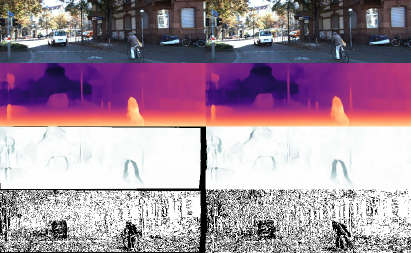
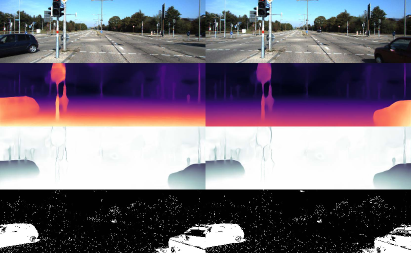
Figure 4: Visual results of depth and masking. Top to bottom: sample image, estimated depth, self-discovered mask $M_{s}$, and auto-mask $M_{a}$ Godard et al. (2019). The proposed $M_{s}$ detects dynamics and occlusions (dark regions), and the binary mask $M_{a}$ finds invalid stationary points (black pixels).

3.2 Photometric and Smoothness Loss

Leveraging brightness constancy and spatial smoothness priors is ubiquitous in classical dense correspondence algorithms Baker & Matthews (2004). Previous works Zhou et al. (2017); Yin & Shi (2018); Ranjan et al. (2019) have used the photometric loss between the warped frame and the reference frame as an unsupervised loss function for network training. With the predicted depth $D_{a}$ and pose $P_{ab}$, we synthesize $I^{\prime}_{a}$ by warping $I_{b}$, where differentiable warping Jaderberg et al. (2015) is used. With the synthesized $I^{\prime}_{a}$ and the reference image $I_{a}$, we formulate the objective function as

$$L_{P}=\frac{1}{|\mathcal{V}|}\sum_{p\in\mathcal{V}}(\lambda\|I_{a}(p)-I^{\prime}_{a}(p)\|_{1}+(1-\lambda)\frac{1-\text{SSIM}_{aa^{\prime}}(p)}{2}),$$ (2)

where $\mathcal{V}$ stands for the set of valid points that are successfully projected from $I_{a}$ to the image plane of $I_{b}$, and $p$ stands for a generic point in $\mathcal{V}$. We choose $L_{1}$ loss due to its robustness to outliers. Besides, $\text{SSIM}_{aa^{\prime}}$ stands for the element-wise similarity between $I_{a}$ and $I^{\prime}_{a}$ by the SSIM function Wang et al. (2004). This is used to better handle complex illumination changes since it normalizes the pixel illumination. More specifically,

$$\text{SSIM (x,y)}=\frac{(2\mu_{x}\mu_{y}+C_{1})(2\sigma_{xy}+C_{2})}{(\mu_{x}^{2}+\mu_{y}^{2}+C_{1})(\sigma_{x}^{2}+\sigma_{y}^{2}+C_{2})},$$ (3)

where $x,y$ stands for two $3$ by $3$ patches around the central pixel. $C_{1}$ and $C_{2}$ are constants. $\mu$ and $\sigma$ are local statistics of the image color, i.e., mean and variance, respectively. Following Godard et al. (2017); Yin & Shi (2018); Ranjan et al. (2019), we use $C_{1}=0.0001$, $C_{2}=0.0009$, and $\lambda=0.15$.

As the photometric loss is not informative in low-texture regions of the scene, existing work also incorporates a smoothness prior to regularize the estimated depth map. We adopt the edge-aware smoothness loss used in Ranjan et al. (2019). Formally,

$$L_{S}=\sum_{p}(e^{-\nabla I_{a}(p)}\cdot\nabla D_{a}(p))^{2},$$ (4)

where $\nabla$ is the first derivative along spatial directions. It ensures smoothness to be guided by image edges.

3.3 Geometry Consistency Loss

To explicitly enforce geometry consistency, we constrain that the predicted $D_{a}$ and $D_{b}$ (related by $P_{ab}$) conform the same 3D structure by penalizing their inconsistency. Specifically, we propose a differentiable depth inconsistency operation to compute the pixel-wise inconsistency between two depth maps, as shown in Fig. 3. Here, $D_{b}^{a}$ is the synthesized depth for $I_{b}$, which is generated by $D_{a}$ and pose $P_{ab}$ with the underlying rigid transformation. $D^{\prime}_{b}$ is an interpolation of $D_{b}$ for aligning and comparing with $D_{b}^{a}$. Given them, we compute the depth inconsistency map $D_{\text{diff}}$ for each $p\in\mathcal{V}$ as:

$$D_{\text{diff}}(p)=\frac{|D_{b}^{a}(p)-D^{\prime}_{b}(p)|}{D_{b}^{a}(p)+D^{\prime}_{b}(p)},$$ (5)

where we normalize depth differences by their summation. This works better than the absolute distance in practice as it treats points at different absolute depths equally in optimization. Besides, the function is symmetric, and the outputs are naturally ranging from $0$ to $1$, which makes the training more stable.

With the inconsistency map, we define the proposed geometry consistency loss as:

$$L_{G}=\frac{1}{|\mathcal{V}|}\sum_{p\in\mathcal{V}}D_{\text{diff}}(p),$$ (6)

which minimizes the geometric inconsistency of predicted depths over two views. By minimizing the depth inconsistency between samples in a batch, we naturally propagate such consistency to the entire sequence: the depth of $I_{1}$ agrees with the depth of $I_{2}$ in a batch; the depth of $I_{2}$ agrees with the depth of $I_{3}$ in another training batch. Eventually, depths of $I_{i}$ of a sequence should all agree with each other, leading to scale-consistent results over the entire sequence.

3.4 Masking Scheme

The assumption of a moving camera and a static scene is underlying in the unsupervised depth learning framework, where the moving objects in the scene and image pairs with identity camera pose provide invalid signals. To be specific, the moving objects create the non-rigid flow that cannot be represented by the depth-based mapping, and the static camera consistently creates the identical flow that is independent to the depth prediction. Therefore, we propose to mask out these regions by introducing a self-discovered mask ($M_{s}$) and adopting the auto-mask ($M_{a}$) by Monodepth2 Godard et al. (2019). The proposed $M_{s}$ computes weights (ranging from $0$ to $1$) for points in $\mathcal{V}$ by checking their depth consistency, and the $M_{a}$ simply removes invalid points from $\mathcal{V}$. The proposed two masks are readily integrated into the proposed learning framework.

3.4.1 Self Discovered Mask

As moving objects and occlusions naturally violate the geometry consistency assumption, they will cause large depth inconsistency in our pre-computed $D_{\text{diff}}$ (Eqn. 5). This encourages us to define the $M_{s}$ as:

$$M_{s}=1-D_{\text{diff}},$$ (7)

where the $M_{s}$ is in $[0,1]$ and it attentively assign low weights for geometrically inconsistent pixels and high weights for consistent pixels.

3.4.2 Auto-Mask

To remove the invalid points in static pairs, e.g., two images are captured at the same position, we use the auto-mask $M_{a}$ that is proposed in Godard et al. (2019). It compares the photometric losses between the mapping by depth and pose and the identity mapping, and it removes the points where the identity mapping leads to a lower loss. Formally, for each $p\in\mathcal{V}$, we have

$$M_{a}(p)=\begin{cases}1&\text{if }\|I_{a}(p)-I^{\prime}_{a}(p)\|_{1}<\|I_{a}(p)-I_{b}(p)\|_{1},\\ 0&\text{otherwise}.\end{cases}$$ (8)

Here $M_{a}$ is a binary mask for each point in $\mathcal{V}$ (valid points), and $I^{\prime}_{a}$ is the warped image from the source image $I_{b}$ using the estimated depth and pose. It makes the network to ignore objects that move at the same velocity as the camera, and it even ignores whole frames when the relative pose is identity.

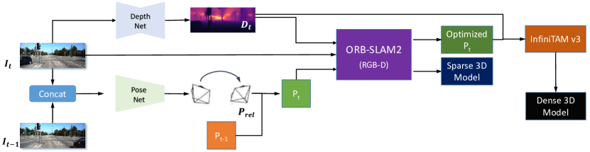
Figure 5: Pipeline of Pseudo-RGBD SLAM. For the current frame $I_{t}$, we first estimate its depth $D_{t}$ using our trained depth CNN. Then, we estimate its relative pose to previous frame $I_{t-1}$ (its pose $P_{t-1}$ has been known in previous tracking) to recover the current pose. Next, we feed the color images, predicted depths, and estimated poses into ORB-SLAM2 Mur-Artal & Tardós (2017), which outputs the accurate camera trajectory and a sparse 3D map. Finally, given the consistent depth and camera trajectory, we construct the dense voxel representation using InfiniTAMv3 Prisacariu et al. (2017). Note that the dense reconstruction here is only used for qualitative demonstration.

3.4.3 How to use masks

First, to use $M_{a}$ in our loss function, we remove invalid points in $\mathcal{V}$ that have $M_{a}(p)=0$. When training the network, we only compute losses on the remaining valid points. Second, we use the proposed $M_{s}$ to re-weight the photometric loss in Eqn. 2 by:

$$L_{P}^{M}=\frac{1}{|\mathcal{V}|}\sum_{p\in\mathcal{V}}(M_{s}(p)\cdot L_{P}(p)).$$ (9)

This mitigates the noisy signals caused by moving objects and occlusions. Fig. 4 shows visual results for the two types of masks, which coincides with our anticipation. The dark regions in $M_{s}$ correspond to moving objects that violate the static scene assumption, e.g., the car region and human ride region. In the binary $M_{a}$, black regions correspond to pixels that have similar speed with the camera, e.g., the moving vehicle in the left example and the static scene in the right example. Tab. 2 shows the ablation study results, which shows that the proposed masks results in a significant performance improvement.

4 Pseudo-RGBD SLAM

In this section, we present a Pseudo-RGBD SLAM system, which is based on our trained models and existing SLAM systems. We overview the system pipeline in Sec. 4.1, followed by elaborating each component in Sec. 4.2, and finally, we discuss the advantages and limitations of the proposed system in Sec. 4.3.

4.1 System Overview

Fig. 5 shows an overview of the proposed method, which is composed of our SC-Depth, ORB-SLAM2 Mur-Artal & Tardós (2017), and InfiniTAMv3 Prisacariu et al. (2017). The whole system takes a monocular RGB video as input and outputs a globally consistent 6-DoF camera trajectory and sparse/dense 3D maps. First, we initialize the tracking and mapping by using the predicted depth on the starting frame $I_{0}$, which creates an initial 3D map. Second, for a new frame $I_{t}$, we estimate its depth and relative pose to the previous view $I_{t-1}$ using our trained networks. As the camera pose of $I_{t-1}$ has been known from previous tracking or initialization, we can obtain the pose estimate for the current view by accumulation. Third, we feed the color image, depth map, and the estimated pose for $I_{t}$ as input into ORB-SLAM2 Mur-Artal & Tardós (2017), which performs matching and optimization, resulting in an optimized camera pose as well as an increased map. In such an incremental way, we eventually obtain a globally consistent camera trajectory and a sparse 3D map from the video. Finally, we feed the color images, depth maps, and camera trajectories into InfiniTAMv3 Prisacariu et al. (2017), which fuses depth maps to construct the dense and textured voxel volumes.

4.2 System Details

ORB-SLAM2.

The original RGB-D system takes the sensor captured depth as input, while we use the estimated depth. It relies on ORB features Rublee et al. (2011) to generate correspondences, and it minimizes the reprojection error for pose optimization. Poor correspondences (beyond the error threshold) are detected and removed as outliers, and the remaining correspondences are used for all sub-tasks, including tracking, mapping, loop closing, and re-localization. We will elaborate on how our predicted depth and pose influence the correspondence and optimization in the system.

Depth.

The predicted depths are used to initialize a 3D map at the beginning, and they are used in the objective function during optimization. Specifically, beyond 2d reprojection error, the system also minimizes the difference between the projected depth (from the 3D map to the image) and the predicted depth. Formally,

$$\begin{cases}E_{2D}=\sqrt{(p_{x}-p^{\prime}_{x})^{2}+(p_{y}-p^{\prime}_{y})^{2}}\\ E_{3D}=\sqrt{(p_{x}-p^{\prime}_{x})^{2}+(p_{y}-p^{\prime}_{y})^{2}+(p_{d}-p^{\prime}_{d})^{2}},\end{cases}$$ (10)

where $p$ stands for points in current image plane, and $p^{\prime}$ stands for points projected from 3D map. $p_{d}$ and $p^{\prime}_{d}$ are their disparities, i.e., inverse depths. Note that $p_{d}$ is computed from our predicted depth map, so it is unavailable in the monocular system. This extends the reprojection error from 2D into 3D, which greatly improves the performance. Consequently, the consistency of estimated depths is vital in tracking. For example, inconsistent depths would increase the reprojection error, and correct matches would be wrongly removed as outliers, which causes the system to fail—See Fig. 9.

Pose.

The predicted pose is used as the initial pose during tracking, in which the system first projects the sparse keypoints in a 3D map to the live view using the estimated pose and then searches for correspondences in the neighboring regions. The camera pose is optimized through the Bundle Adjustment Mur-Artal & Tardós (2017). After tracking, we enrich the 3D map by unprojecting the keypoints detected in the live view to the map using the optimized camera pose. The original ORB-SLAM2 uses the constant velocity motion model for initial pose, which simply assumes that the camera motion is the same as the previous frame. Formally,

$$T_{t\rightarrow t+1}=\begin{cases}T_{t-1\rightarrow t}&\text{ORB-SLAM2},\\ \text{PoseNet}(I_{t},I_{t+1})&\text{Ours},\end{cases}$$ (11)

where $T$ stands for relative pose. However, this assumption is often violated in real scenarios, such as abrupt motion in driving scenes. Though these frames are few in the sequence, they usually contribute the most of the drift in the final evaluation. Our trained pose CNN has the potential to cope with these cases.

InfiniTAMv3.

It takes RGB-D videos and can densely reconstruct the scene structure. We disable the internal tracking module and use our optimized camera poses and predicted depths for reconstruction. This is only used for visualization purposes, and it is also a demonstration of our consistent results. Note that the dense reconstruction is very sensitive to geometry consistency, i.e., it will crash when depths are not sufficiently consistent. Fig. 11 shows the screenshot of our demo, which can be found in the supplementary material.

4.3 Discussion

Our proposed SLAM system leverages the advantage of deep learning, and it optimizes the predicted poses in the multi-view geometry-based framework. This has distinctive advantages over existing solutions.

Advantages.

Compared with classical monocular SLAM systems such as ORB-SLAM2 Mur-Artal & Tardós (2017), our advantages include:

1. ORB-SLAM2 is often hard to initialize because it requires the multi-view triangulation, while our method can initialize at any time without latency by using the estimated dense depth—See Fig. 9.

2. ORB-SLAM2 often loses tracking when the 3D map is over-sparse, while our method is more robust because we can enrich the map by using the predicted dense depth—See Fig. 9.

3. ORB-SLAM2 can only provide a sparse map, while our method enables dense 3D reconstruction by using the predicted dense depth—See Fig. 12.

Compared with learning-based methods Li et al. (2018), our advantage is the post geometric optimization e.g., Loop Closing Mur-Artal & Tardós (2014), which can effectively correct drifts and improve the performance, as shown in Fig. 8.

Limitations.

Our method cannot recover the absolute scale because only monocular videos are used. However, in real-world applications, the metric scale can be recovered by using other sensors and cues, like IMU and road landmarks.

5 Experiments

5.1 Implementation details

Network architecture.

Our depth network takes a single RGB image as input and outputs an inverse depth map. It is a U-Net structure Ronneberger et al. (2015), and we use the ResNet50 He et al. (2016) encoder to extract features. The decoder is the DispNet as used in Zhou et al. (2017). The activations are sigmoids at the output layer and ELU nonlinearities Clevert et al. (2015) elsewhere. We convert the sigmoid output $x$ to depth with $D=1/(ax+b)$, where $a$ and $b$ are chosen to constrain $D$ between 0.1 and 100 units. It is a widely assumed depth range for outdoor driving scenes, which is the same with all related works Zhou et al. (2017); Yin & Shi (2018); Ranjan et al. (2019). Besides, our pose network accepts two RGB frames as input and outputs their 6D relative camera pose. We use the ResNet18 He et al. (2016) encoder to extract features. In order to accept two frames, we modify the first layer to have six channels. Then features are decoded to 6-DoF parameters via four convolutional layers.

Single scale supervision.

Previous methods compute the losses on an image pyramid, i.e., usually four layers. They either work on the decoder’s side outputs Zhou et al. (2017); Yin & Shi (2018); Zou et al. (2018) or upsample them to the original image resolution Godard et al. (2019). However, it introduces great computational overhead in training. By contrast, we only compute the loss on the original image resolution. This has a less computational cost and achieves on par performance with the multi-scale solution in MonoDepth2 Godard et al. (2019), as shown in Tab. 2. The motivation is that we empirically find that the supervision on low-resolution images is inaccurate, and the camera movement between training image pairs is small so that the multi-scale solution is unnecessary.

Training details.

We implement the proposed method using the PyTorch Paszke et al. (2017). Following Zhou et al. (2017); Ranjan et al. (2019); Wang et al. (2018), we use a snippet of three sequential video frames as a training sample. We compute the projection and losses from the second frame to others and reverse them again for maximizing the data usage. The images are augmented with random scaling, cropping, and horizontal flips during training. We use ADAM Kingma & Ba (2014) optimizer and set the learning rate to be $10^{-4}$. During training, we set $\alpha=1.0$, $\beta=0.1$, and $\gamma=0.5$ in Eqn. 1. For fast convergence, we initialize the encoder of our networks by using the pre-trained model on ImageNet Deng et al. (2009).

Table 1: Single-view depth estimation results on KITTI Geiger et al. (2013). Legends: D—depth supervision; S—stereo pairs; M—monocular snippets; L—semantic labels or networks; F—joint learning with optical flow.

			Error $\downarrow$				Accuracy $\uparrow$
Methods	Resolution	Supervision	AbsRel	SqRel	RMS	RMSlog	$\delta_{1}$	$\delta_{2}$	$\delta_{3}$
Eigen et al. (2014)	$612\times 184$	D	0.203	1.548	6.307	0.282	0.702	0.890	0.958
Kuznietsov et al. (2017)	$621\times 187$	S+D	0.113	0.741	4.621	0.189	0.862	0.960	0.986
DORN Fu et al. (2018)	$513\times 385$	D	0.072	0.307	2.727	0.120	0.932	0.984	0.994
VNL Yin et al. (2019)	$385\times 385$	D	0.072	-	3.258	0.117	0.938	0.990	0.998
Garg et al. (2016)	$620\times 188$	S	0.152	1.226	5.849	0.246	0.784	0.921	0.967
Godard et al. (2017)	$512\times 256$	S	0.148	1.344	5.927	0.247	0.803	0.922	0.964
Zhan et al. (2018)	$608\times 160$	S+M	0.144	1.391	5.869	0.241	0.803	0.928	0.969
SuperDepth+pp Pillai et al. (2019)	$1024\times 382$	S	0.112	0.875	4.958	0.207	0.852	0.947	0.977
Monodepth2-SGodard et al. (2019)	$1024\times 320$	S	0.107	0.849	4.764	0.201	0.874	0.953	0.977
Monodepth2-MSGodard et al. (2019)	$1024\times 320$	S+M	0.106	0.806	4.630	0.193	0.876	0.958	0.980
D3VO Yang et al. (2020)	$512\times 256$	S+M	0.099	0.763	4.485	0.185	0.885	0.958	0.979
Geonet-Resnet Yin & Shi (2018)	$416\times 128$	M+F	0.155	1.296	5.857	0.233	0.793	0.931	0.973
DF-Net Zou et al. (2018)	$576\times 160$	M+F	0.150	1.124	5.507	0.223	0.806	0.933	0.973
Struct2Depth Casser et al. (2019a)	$416\times 128$	M+L	0.141	1.026	5.291	0.215	0.816	0.945	0.979
DWGordon et al. (2019)	$416\times 128$	M+L	0.128	0.959	5.230	0.212	0.845	0.947	0.976
GLNetChen et al. (2019b)	$416\times 128$	M+F	0.135	1.070	5.230	0.210	0.841	0.948	0.980
CC Ranjan et al. (2019)	$832\times 256$	M+F	0.140	1.070	5.326	0.217	0.826	0.941	0.975
EPC++ Luo et al. (2019)	$832\times 256$	M+F	0.141	1.029	5.350	0.216	0.816	0.941	0.976
Zhao et al. (2020)	$832\times 256$	M+F	0.113	0.704	4.581	0.184	0.871	0.961	0.984
Insta-DM Lee et al. (2021)	$832\times 256$	M+F+L	0.112	0.777	4.772	0.191	0.872	0.959	0.982
SGDepth-full Klingner et al. (2020)	$1280\times 384$	M+L	0.107	0.768	4.468	0.186	0.891	0.963	0.982
PackNet-Sem Guizilini et al. (2020b)	$1280\times 384$	M+L	0.100	0.761	4.270	0.175	0.902	0.965	0.982
SfMLearner Zhou et al. (2017)	$416\times 128$	M	0.208	1.768	6.856	0.283	0.678	0.885	0.957
Yang et al. (2018b)	$416\times 128$	M	0.182	1.481	6.501	0.267	0.725	0.906	0.963
Vid2Depth Mahjourian et al. (2018)	$416\times 128$	M	0.163	1.240	6.220	0.250	0.762	0.916	0.968
DDVO Wang et al. (2018)	$416\times 128$	M	0.151	1.257	5.583	0.228	0.810	0.936	0.974
Zhou et al. (2019)	$1248\times 384$	M	0.121	0.837	4.945	0.197	0.853	0.955	0.982
MonoDepth2 Godard et al. (2019)	$1024\times 320$	M	0.115	0.882	4.701	0.190	0.879	0.961	0.982
Li et al. (2020)	$416\times 128$	M	0.130	0.950	5.138	0.209	0.843	0.948	0.978
PackNet-SfM Guizilini et al. (2020a)	$1280\times 384$	M	0.107	0.802	4.538	0.186	0.889	0.962	0.981
Ours-R18	$416\times 128$	M	0.132	0.982	5.226	0.209	0.835	0.947	0.978
Ours-R50	$416\times 128$	M	0.126	0.920	5.245	0.208	0.840	0.949	0.979
Ours-R18	$832\times 256$	M	0.119	0.857	4.950	0.197	0.863	0.957	0.981
Ours-R50	$832\times 256$	M	0.114	0.813	4.706	0.191	0.873	0.960	0.982

Table 2: Ablation study results on KITTI. We use the ResNet18 model, and the image resolution is $416\times 128$.

Models	AbsRel	$\delta_{1}$	Time
Baseline (B)	0.200	0.786	10h
B+$L_{G}$	0.155	0.786
B+$L_{G}$+$M_{s}$	0.137	0.822
B+$L_{G}$+$M_{a}$	0.153	0.797
B+$L_{G}$+$M_{s}$+$M_{a}$ (Ours)	0.132	0.835
Ours with NCC	0.145	0.804	11h
Ours + Multi-Scale	0.134	0.829	21h

Table 3: Trade-offs between image resolution, network, and speed. We train models on KITTI using a TESLA V100 GPU and test the inference speed in an RTX 2080 GPU.

Resolution	Model	AbsRel	$\delta_{1}$	Train	Infer
$416\times 128$	R18	0.132	0.835	10h	228 fps
	R50	0.126	0.840	16h	110 fps
$832\times 256$	R18	0.119	0.863	29h	133 fps
	R50	0.114	0.873	37h	59 fps

Table 4: Single-view depth estimation results on NYUv2 Silberman et al. (2012). Legends: D—depth supervision; M—unsupervised training using monocular snippets; F—joint learning with the optical flow; WR—weak rectification Bian et al. (2020) which pre-processes the hand-held camera captured videos for better training. More specifically, Bian et al. (2020) remove the relative rotation between training pairs since they find that it is hard for the pose network to learn image rotation.

Methods	Resolution	Supervision	Error $\downarrow$			Accuracy $\uparrow$
			AbsRel	Log10	RMS	$\delta_{1}$	$\delta_{2}$	$\delta_{3}$
Make3D Saxena et al. (2006)	-	D	0.349	-	1.214	0.447	0.745	0.897
Wang et al. (2015)	-	D	0.220	0.094	0.745	0.605	0.890	0.970
Eigen & Fergus (2015)	$320\times 240$	D	0.158	-	0.641	0.769	0.950	0.988
Chakrabarti et al. (2016)	$561\times 427$	D	0.149	-	0.620	0.806	0.958	0.987
Laina et al. (2016)	$304\times 228$	D	0.127	0.055	0.573	0.811	0.953	0.988
Li et al. (2017)	$310\times 232$	D	0.143	0.063	0.635	0.788	0.958	0.991
DORN Fu et al. (2018)	$353\times 257$	D	0.115	0.051	0.509	0.828	0.965	0.992
VNL Yin et al. (2019)	$385\times 385$	D	0.108	0.048	0.416	0.875	0.976	0.994
Zhou et al. (2019)	$256\times 192$	M+F	0.208	0.086	0.712	0.674	0.900	0.968
Zhao et al. (2020)	$576\times 448$	M+F	0.189	0.079	0.686	0.701	0.912	0.978
Monodepth2 Godard et al. (2019)	$320\times 256$	M	0.176	0.074	0.639	0.734	0.937	0.983
Ours-R18	$320\times 256$	M	0.159	0.068	0.608	0.772	0.939	0.982
Ours-R50	$320\times 256$	M	0.157	0.067	0.593	0.780	0.940	0.984
Monodepth2 Godard et al. (2019)	$320\times 256$	WR-M	0.151	0.064	0.559	0.795	0.947	0.985
Ours-R18	$320\times 256$	WR-M	0.143	0.060	0.538	0.812	0.951	0.986
Ours-R50	$320\times 256$	WR-M	0.142	0.060	0.529	0.813	0.952	0.987

Datasets.

For depth estimation evaluation, we use both the KITTI Geiger et al. (2013) and NYUv2 Silberman et al. (2012) datasets. In KITTI, we use the same training/testing split as in Zhou et al. (2017). The 697 images are used for testing. We train the network for $200K$ iterations, where we set the batch size to be $4$ and resize images to $832\times 256$ resolution for training. In NYUv2, we use the officially provided 654 densely labeled images for testing, and use the rest sequences (no overlapping with the testing scenes) for training. We extract one frame from every $10$ frame in the original video to remove redundant frames, and we resize images to $320\times 256$ resolution as input of the network. We train models for $50$ epochs, and the batch size is $8$. For visual odometry evaluation, we use the KITTI odometry dataset (Seq. 00-08) for training, and we test our method on the Seq. 09-10. Moreover, we use the KAIST urban dataset Jeong et al. (2019) to validate the zero-shot generalization ability of our method. We use one of the hardest scenes (urban39-pankyo), which contains more than $18000$ street-view images, and we split it into $9$ sequences with each sequence containing $2000$ images for testing.

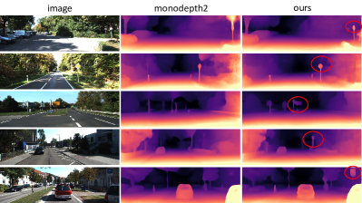
Figure 6: Qualitative comparison with the Monodepth2 Godard et al. (2019) on KITTI.

Evaluation metrics.

For depth evaluation, following previous methods Yin et al. (2019); Zhou et al. (2017), we use the mean absolute relative error (AbsRel), mean log10 error (Log10), root mean squared error (RMS), root mean squared log error (RMSlog), and the accuracy under threshold ($\delta_{i}$ $<$ $1.25^{i}$, $i=1,2,3$). As unsupervised methods cannot recover the absolute scale, we multiply the predicted depth maps by a scalar that matches the median with that of the ground truth, as in Zhou et al. (2017). The predicted depths are capped at $80m/10m$ in KITTI and NYUv2 datasets, respectively. For visual odometry evaluation, we follow the standard evaluation metrics, including the translational ($t_{err}$) and rotational errors ($r_{err}$) averaged over the entire sequence Geiger et al. (2013), and the absolute trajectory error (ATE) Sturm et al. (2012).

5.2 Depth Estimation

Results on KITTI.

Tab. 1 shows the results, which shows that the supervised methods Fu et al. (2018); Yin et al. (2019) are best-performing, followed by the stereo trained models Yang et al. (2020). Besides, it shows that learning with semantic labels Guizilini et al. (2020b) or optical flow Zhao et al. (2020) can effectively improve the performance of monocular methods. We are here more interested in the monocular methods that do not use additional information. In this category, our method outperforms previous methods (before 2020), and it shows on par performance with the MonoDepth2 Godard et al. (2019). However, we argue that our advantage against Monodepth2 is the depth consistency (Tab. 6), which has important implications on downstream video-based tasks. For example, contributed to the consistent depth prediction, our method can be readily plugged into the Visual SLAM systems, while the Monodepth2 is unable—See Fig. 9 for detailed analysis.

Efficacy of the proposed methods.

Tab. 2 summarizes the results. It shows that the proposed $L_{G}$ makes training more stable by enforcing depth consistency, and the proposed $M_{s}$ can boost performance significantly by handling scene dynamics. Besides, it shows that using $M_{a}$ can contribute to extra marginal performance improvement by removing the stationary points. Consequently, the final solution (with all terms) can achieve the best performance. Moreover, Tab. 3 shows the relation between depth accuracy, training time, inference speed, network architecture, and image resolution.

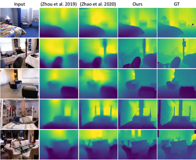
Figure 7: Qualitative comparison with the state-of-the art unsupervised methods on NYUv2.

Table 5: Visual odometry results on KITTI Geiger et al. (2013). S/M stands for training on stereo/monocular videos, and G stands for geometric optimization. ✗ stands for failure in initialization or tracking.

Methods	Types	Seq. 09			Seq. 10
		$t_{err}$ ($\%$)	$r_{err}$ (${}^{\circ}/100m$)	ATE(m)	$t_{err}$ ($\%$)	$r_{err}$ (${}^{\circ}/100m$)	ATE(m)
Depth-VO-Feat Zhan et al. (2018)	S	11.89	3.60	52.12	12.82	3.41	24.70
UndeepVO Li et al. (2018)	S	7.01	3.60	-	10.63	4.60	-
PoseGraph Li et al. (2019a)	S + G	6.23	2.11	-	12.9	3.17	-
DVSO Yang et al. (2018b)	S + G	0.83	0.21	-	0.74	0.21	-
D3VO Yang et al. (2020)	S + G	0.78	-	-	0.62	-	-
SfMLearner Zhou et al. (2017)	M	19.15	6.82	77.79	40.40	17.69	67.34
GeoNet Yin & Shi (2018)	M	28.72	9.8	158.45	23.90	9.0	43.04
DeepMatchVO Shen et al. (2019)	M	9.91	3.8	27.08	12.18	5.9	24.44
MonoDepth2 Godard et al. (2019)	M	17.17	3.85	76.22	11.68	5.31	20.35
DW Gordon et al. (2019)-Learned	M	-	-	20.91	-	-	17.88
DW Gordon et al. (2019)-Corrected	M	-	-	19.01	-	-	14.85
Zou et al. (2020)	M	3.49	1.00	11.30	5.81	1.8	11.80
Zhao et al. (2020)	M + G	6.93	0.44	-	4.66	0.62	-
SC-Depth (Ours w/o $L_{G}$)	M	12.43	4.65	83.27	11.86	4.95	21.19
SC-Depth (Ours)	M	7.31	3.05	23.56	7.79	4.90	12.00
Pseudo-RGBD SLAM (MonoDepth2)	M + G	✗	✗	✗	✗	✗	✗
Pseudo-RGBD SLAM (Ours w/o $L_{G}$)	M + G	7.81	2.44	34.15	7.62	2.41	9.02
Pseudo-RGBD SLAM (Ours - Motion Model)	M + G	5.70	1.33	13.22	3.82	1.76	5.96
Pseudo-RGBD SLAM (Ours - Pose CNN)	M + G	5.08	1.05	13.40	4.32	2.34	7.99

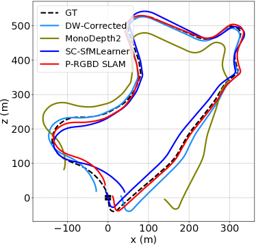
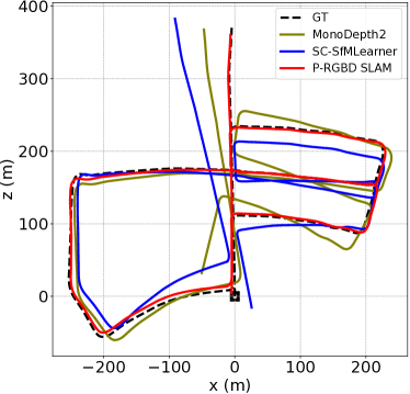
Figure 8: Estimated trajectory on Seq. 09 (left) and 05 (right). The results optimized by the proposed Pseudo-RGBD SLAM are more accurate than our SC-Depth and other learning-based methods, and the improvement is especially large when loops are detected and closed. For example, the $t_{err}$ is reduced from $5.91$ to $1.67$ on Seq. 05.

Multi-scale supervision.

Tab. 2 shows the results of our method with the modified multi-scale solution proposed in Godard et al. (2019). It upsamples the predicted four depth maps to original image resolution and then computes losses instead of downsampling the original color image Zhou et al. (2017). The result demonstrates that our method could hardly benefit from that, and it requires two times longer time for training. Therefore, we use single-scale supervision in our framework.

SSIM vs NCC.

Tab. 2 shows the results of our method with the normalized cross-correlation (NCC) loss, in which we replace the SSIM. Both losses compute the local image similarity on a 3 by 3 patch. The results show that SSIM leads to better performance than NCC in our unsupervised learning framework.

Results on NYUv2.

Tab. 4 shows the results, which shows that our method outperforms previous unsupervised methods by a large margin. Besides, following Bian et al. (2020), we remove the relative rotation between training image pairs since they find that it is hard for the pose network to learn image rotation. This leads to a significant improvement because rotation is the dominate ego-motion in hand-held camera captured videos. Zhao et al. (2020) solves the problem by replacing the Pose CNN with a traditional geometry-based pose solver. The qualitative results are shown in Fig. 7. We find that MonoDepth2 Godard et al. (2019) often collapses in training, so we report the best result. Compared with the supervised methods, our method is inferior to the state-of-the-art Yin et al. (2019) but outperforms many previous methods Liu et al. (2016); Saxena et al. (2006); Wang et al. (2015); Eigen & Fergus (2015); Chakrabarti et al. (2016); Li et al. (2017).

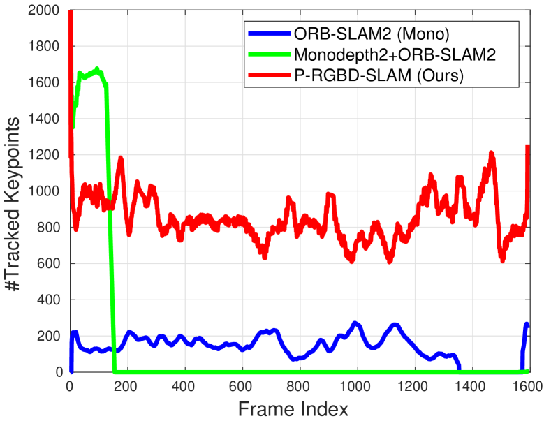
Figure 9: Number of tracked keypoints on Seq. 09. We extract $2000$ feature points for all methods, and the values in the figure are smoothed for visualization.

Table 6: Depth consistency results on Seq. 09. Fitness measures the overlapping area of two point clouds (# of inlier correspondences / # of points in target). RMSE is averaged over all inlier correspondences (#Corr).

Methods	Fitness ($\uparrow$)	RMSE ($\downarrow$)	#Corr ($\uparrow$)
MonoDepth2	0.384	9.84e-3	80.776K
Ours (w/o $L_{G}$)	0.663	8.90e-3	129.825K
Ours	0.689	8.71e-3	134.956K

Table 7: Visual odometry results on KITTI. We evaluate the results on all frames and on keyframes that are selected by the ORB-SLAM2 since the latter cannot provide results for the full sequence due to unsuccessful initialization or tracking failure. The ATE (m) metric is used. We use $2K$ keypoints as default, and we analyze the effect of keypoint numbers on system performance by increasing it to $8K$.

	ORB KeyFrames			All Frames
Seq	Frames	ORB	Ours	Frames	Ours-2K	Ours-8K
00	1928	6.33	6.43	4541	6.05	6.57
01	395	468.9	299.11	1101	289.29	301.08
02	2445	26.18	8.86	4661	8.79	9.42
03	361	1.21	2.92	801	3.00	3.71
04	149	1.73	2.75	271	2.64	2.89
05	1129	4.78	4.47	2761	4.35	5.58
06	479	13.34	4.11	1101	4.35	6.10
07	467	2.28	0.77	1101	0.76	2.39
08	2129	49.23	18.48	4071	19.37	20.10
09	871	50.78	13.43	1591	13.40	17.16
10	549	7.26	7.52	1201	7.99	6.48

Table 8: Zero-short generalization on KAIST dataset Jeong et al. (2019). We compare our method with ORB-SLAM2 using the ATE (m) metric.

	ORB KeyFrames			All Frames (2K)
Seq	Frames	ORB	Ours	Ours
00	189	7.04	2.35	2.21
01	286	21.06	3.90	4.29
02	231	11.95	4.65	5.11
03	150	11.67	2.71	2.59
04	140	3.80	2.00	1.67
05	201	55.87	27.46	28.34
06	306	136.85	7.47	7.78
07	304	10.41	16.27	16.48
08	185	2.48	1.66	1.44

5.3 Visual Odometry

Comparing with deep learning based methods.

Tab. 5 shows the visual odometry results on KITTI. For methods that train on monocular videos, we align the scale of their predicted results with the ground truth by using the 7-DoF optimization. The results show that the proposed SC-Depth outperforms the previous monocular alternatives, and it even shows on par performance with the stereo trained method Li et al. (2018). However, it is not as good as the very recent approach Zou et al. (2020) that models the long-term geometry by using the LSTM module. Besides, the results show that the proposed Pseudo-RGBD SLAM system improves the accuracy significantly over our SC-Depth, which is contributed to the geometric optimization. The success of D3VO Yang et al. (2020) also confirms the importance of geometric optimization for odometry accuracy. However, note that stereo-trained methods can estimate depths at the metric scale, which are readily optimized in existing SLAM frameworks. By contrast, the monocular trained methods suffer from the scale inconsistency issue, which makes the post-optimization non-trivial—See Fig. 9. Our contribution here is enabling the monocular trained methods to predict the scale consistent results so that it allows for optimizing the predicted depths and poses by using the classical geometric frameworks. A qualitative comparison is provided in Fig. 8, which shows that the trajectory optimized by our Pseudo-RGBD SLAM is more well-aligned with the ground truth than our SC-Depth and other learning-based methods.

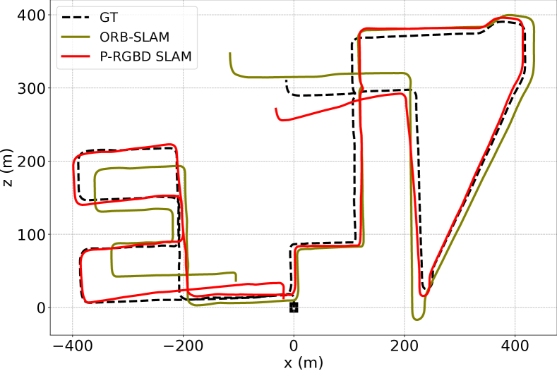
Figure 10: Estimated trajectory on Seq. 08. ORB-SLAM2 is hard to maintain consistent scales over a long video (e.g., left is small, and right is big), while our method is able by leveraging the scale-consistent depth prediction.

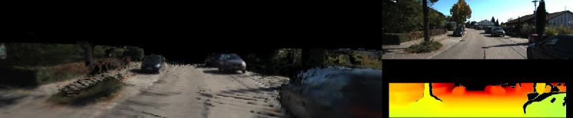
Figure 11: Dense multi-view reconstruction on Seq. 09. The left column shows the reconstructed 3D voxels. The right column shows the input RGB image, estimated depth map. We use the depth CNN trained on Seq. 00-08, and the predicted depth is cropped and masked by using our proposed $M_{s}$.

Depth consistency evaluation.

We evaluate the geometry consistency of predicted depths by using the point cloud registration metric that is implemented in the Open3D library Zhou et al. (2018). To be specific, we use the “open3d.registration.evaluate_registration” function. It computes the RMSE of two aligned point clouds and recognizes the inlier correspondences by a constant threshold. Then it measures the overlapping area of point clouds by counting the ratio of inlier correspondences in all the target points. More details can be founded in the Open3D library. For a given testing sequence, we predict the depth and relative pose for every adjacent image pair, and we convert the depth into point clouds for evaluation, where all the depth maps are resized to $832\times 256$ resolution for a fair comparison. Tab. 6 shows the results, where we compare our method with Monodepth2 Godard et al. (2019). It shows that our predicted depths are significantly more consistent than the latter, and we hypothesize this is the reason why our method can be readily plugged into the ORB-SLAM2 system while the Monodepth2 fails. We conduct a more detailed comparison by reporting the number of tracked keypoints in each frame. The results are shown in Fig. 9.

Pose network or motion model.

Tab. 5 shows the results, where using the built-in motion model in ORB-SLAM or using our pose CNN for pose initialization leads to similar performance. We conjecture the reason is that the motion model is satisfied in most driving scenarios, where forward motion is dominant. However, we believe that using the pose network is a more general solution because the constant velocity model is violated when abrupt motion occurs.

Comparing with ORB-SLAM2.

Tab. 7 shows the odometry results on KITTI Geiger et al. (2013). We evaluate results on all frames and on keyframes that are selected by ORB-SLAM2 Mur-Artal & Tardós (2017), since the latter cannot provide results for the full sequence due to unsuccessful initialization or tracking failure. The results on eleven sequences show that our method either achieves on par accuracy with the ORB-SLAM2 or significantly outperforms the latter. Besides tracking accuracy, our system is more robust than the ORB-SLAM2. A detailed comparison is provided in Fig. 9, where our method always tracks more points than the latter (e.g., about $800$ vs $100$). Moreover, we find that ORB-SLAM2 sometimes suffers from heavy scale drifts in long sequences—See Fig. 10 where ORB-SLAM2 provides inconsistent scales between left and right parts. In this scenario, our method can maintain a consistent scale over the entire sequence by leveraging the scale-consistent depth prediction.

Using more or less keypoints.

Tab. 7 shows the ablation study results, where our system with $2K$ keypoints is more accurate than that with $8K$ keypoints. We conjecture the reason is that using more keypoints would also introduce more outliers, while the geometric optimization requires only a few accurate sparse points. We hence recommend users choosing keypoint numbers by considering the trade-off between the system accuracy and robustness (Fig. 9).

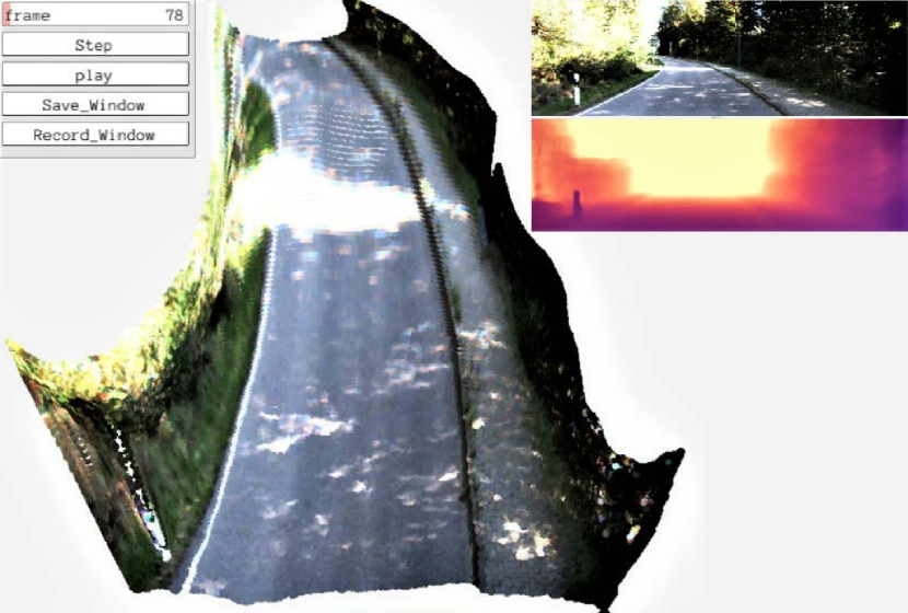
Figure 12: Point cloud visualization on Seq. 09. For each incoming image (right 1st row), we predict the depth map (right 2nd row) using our trained network and convert it to a 3D point cloud, which is rendered using the color image and visualized in an eye-bird view (left).

Zero-short generalization.

We validate the generalization ability of our proposed Pseudo-RGBD SLAM on KAIST urban dataset Jeong et al. (2019), where our models are trained on KITTI. The results are reported in Tab. 8. It shows that our method consistently outperforms ORB-SLAM2, which demonstrates the robustness of our proposed system. Moreover, we demonstrate the generalization ability of our method by presenting a real-world demo—See Fig. 1.

5.4 Qualitative Evaluation

We provide several demos in the supplementary material, which are briefly described below.

Per-frame 3D visualization.

Fig. 12 shows the visualization for predicted depths and textured point clouds on Seq. 09. We use the model trained on Seq. 00-08. This demo is to show that the predicted scene or object structure by our trained depth CNN is visually reasonable, and their scales are consistent over time. Note that inconsistent prediction would cause flickering videos, while it is doesn’t occur in our demo.

Dense multiple view reconstruction.

Fig. 11 shows our dense reconstruction demo. As the depth range is wild in outdoor scenes, we have to reduce the voxel size of TSDF Curless & Levoy (1996) for affording the memory requirement, which degrades the reconstruction quality. Although the reconstruction is inferior to the state-of-the-art methods, this demo clearly demonstrates the high consistency of our estimated depths.

Generalization on real-world videos.

Fig. 1 shows the depth and camera trajectory generated by our method on a self-captured driving video. The video is captured in Adelaide, Australia. We use a single camera, which is mounted on a driving car. Due to the lack of an accurate ground truth trajectory, we use the Google map for qualitative evaluation. The scene is so challenging that ORB-SLAM2 Mur-Artal & Tardós (2017) is unable to generate a complete trajectory, while the proposed Pseudo-RGBD SLAM performs well.

6 Conclusion

This paper proposes a video-based unsupervised depth learning method. Thanks to the proposed geometry consistency loss and masking scheme, our trained network can predict scale-consistent and accurate depths over a video. The depth accuracy is comprehensively evaluated in both indoor and outdoor scenes, and the quantitative results are attached. Besides, we demonstrate better consistency against the related work which shows on par depth accuracy to our method, and we show that such consistency enables our method to be readily plugged into the existing Visual SLAM system. This shows the possibility of leveraging the depth network that is unsupervised trained from monocular videos for camera tracking and dense reconstruction.

References

- Baker & Matthews (2004) Baker, S., & Matthews, I. (2004). Lucas-kanade 20 years on: A unifying framework. International Journal on Computer Vision (IJCV), 56(3).
- Bian et al. (2019a) Bian, J., Lin, W.-Y., Liu, Y., Zhang, L., Yeung, S.-K., Cheng, M.-M., et al. (2019a). GMS: Grid-based motion statistics for fast, ultra-robust feature correspondence. International Journal on Computer Vision (IJCV).
- Bian et al. (2019b) Bian, J.-W., Li, Z., Wang, N., Zhan, H., Shen, C., Cheng, M.-M., et al. (2019b). Unsupervised scale-consistent depth and ego-motion learning from monocular video. In Neural Information Processing Systems (NeurIPS).
- Bian et al. (2019c) Bian, J.-W., Wu, Y.-H., Zhao, J., Liu, Y., Zhang, L., Cheng, M.-M., et al. (2019c). An evaluation of feature matchers for fundamental matrix estimation. In British Machine Vision Conference (BMVC).
- Bian et al. (2020) Bian, J.-W., Zhan, H., Wang, N., Chin, T.-J., Shen, C., & Reid, I. (2020). Unsupervised depth learning in challenging indoor video: Weak rectification to rescue. arXiv preprint arXiv:2006.02708.
- Bloesch et al. (2018) Bloesch, M., Czarnowski, J., Clark, R., Leutenegger, S., & Davison, A. J. (2018). Codeslam—learning a compact, optimisable representation for dense visual slam. In IEEE Conference on Computer Vision and Pattern Recognition (CVPR). (pp. 2560–2568).
- Butler et al. (2012) Butler, D. J., Wulff, J., Stanley, G. B., & Black, M. J. (2012). A naturalistic open source movie for optical flow evaluation. In European Conference on Computer Vision (ECCV). (pp. 611–625).
- Casser et al. (2019a) Casser, V., Pirk, S., Mahjourian, R., & Angelova, A. (2019a). Depth prediction without the sensors: Leveraging structure for unsupervised learning from monocular videos. In Association for the Advancement of Artificial Intelligence (AAAI).
- Casser et al. (2019b) Casser, V., Pirk, S., Mahjourian, R., & Angelova, A. (2019b). Unsupervised monocular depth and ego-motion learning with structure and semantics. In CVPR Workshop on Visual Odometry and Computer Vision Applications Based on Location Cues (VOCVALC).
- Chakrabarti et al. (2016) Chakrabarti, A., Shao, J., & Shakhnarovich, G. (2016). Depth from a single image by harmonizing overcomplete local network predictions. In Neural Information Processing Systems (NeurIPS).
- Chen et al. (2019a) Chen, W., Qian, S., & Deng, J. (2019a). Learning single-image depth from videos using quality assessment networks. In IEEE Conference on Computer Vision and Pattern Recognition (CVPR). (pp. 5604–5613).
- Chen et al. (2019b) Chen, Y., Schmid, C., & Sminchisescu, C. (2019b). Self-supervised learning with geometric constraints in monocular video: Connecting flow, depth, and camera. In IEEE International Conference on Computer Vision (ICCV). (pp. 7063–7072).
- Clevert et al. (2015) Clevert, D.-A., Unterthiner, T., & Hochreiter, S. (2015). Fast and accurate deep network learning by exponential linear units (elus). arXiv preprint arXiv:1511.07289.
- Curless & Levoy (1996) Curless, B., & Levoy, M. (1996). A volumetric method for building complex models from range images. In ACM Transactions on Graphics (SIGGRAPH). CUMINCAD.
- Deng et al. (2009) Deng, J., Dong, W., Socher, R., Li, L.-J., Li, K., & Fei-Fei, L. (2009). ImageNet: A Large-Scale Hierarchical Image Database. In IEEE Conference on Computer Vision and Pattern Recognition (CVPR).
- Eigen & Fergus (2015) Eigen, D., & Fergus, R. (2015). Predicting depth, surface normals and semantic labels with a common multi-scale convolutional architecture. In IEEE International Conference on Computer Vision (ICCV).
- Eigen et al. (2014) Eigen, D., Puhrsch, C., & Fergus, R. (2014). Depth map prediction from a single image using a multi-scale deep network. In Neural Information Processing Systems (NeurIPS).
- Engel et al. (2017) Engel, J., Koltun, V., & Cremers, D. (2017). Direct sparse odometry. IEEE Transactions on Pattern Recognition and Machine Intelligence (TPAMI), 40(3), pp. 611–625.
- Forster et al. (2014) Forster, C., Pizzoli, M., & Scaramuzza, D. (2014). Svo: Fast semi-direct monocular visual odometry. In IEEE International Conference on Robotics and Automation (ICRA). IEEE, (pp. 15–22).
- Fu et al. (2018) Fu, H., Gong, M., Wang, C., Batmanghelich, K., & Tao, D. (2018). Deep ordinal regression network for monocular depth estimation. In IEEE Conference on Computer Vision and Pattern Recognition (CVPR). (pp. 2002–2011).
- Garg et al. (2016) Garg, R., BG, V. K., Carneiro, G., & Reid, I. (2016). Unsupervised cnn for single view depth estimation: Geometry to the rescue. In European Conference on Computer Vision (ECCV). Springer.
- Garg et al. (2019) Garg, R., Wadhwa, N., Ansari, S., & Barron, J. T. (2019). Learning single camera depth estimation using dual-pixels. In IEEE International Conference on Computer Vision (ICCV). (pp. 7628–7637).
- Geiger et al. (2013) Geiger, A., Lenz, P., Stiller, C., & Urtasun, R. (2013). Vision meets Robotics: The kitti dataset. International Journal of Robotics Research (IJRR).
- Geiger et al. (2011) Geiger, A., Ziegler, J., & Stiller, C. (2011). Stereoscan: Dense 3d reconstruction in real-time. In Intelligent Vehicles Symposium (IV).
- Godard et al. (2017) Godard, C., Mac Aodha, O., & Brostow, G. J. (2017). Unsupervised monocular depth estimation with left-right consistency. In IEEE Conference on Computer Vision and Pattern Recognition (CVPR).
- Godard et al. (2019) Godard, C., Mac Aodha, O., Firman, M., & Brostow, G. J. (2019). Digging into self-supervised monocular depth prediction. In IEEE International Conference on Computer Vision (ICCV).
- Gordon et al. (2019) Gordon, A., Li, H., Jonschkowski, R., & Angelova, A. (2019). Depth from videos in the wild: Unsupervised monocular depth learning from unknown cameras. In IEEE International Conference on Computer Vision (ICCV).
- Guizilini et al. (2020a) Guizilini, V., Ambrus, R., Pillai, S., Raventos, A., & Gaidon, A. (2020a). 3d packing for self-supervised monocular depth estimation. In IEEE Conference on Computer Vision and Pattern Recognition (CVPR).
- Guizilini et al. (2020b) Guizilini, V., Hou, R., Li, J., Ambrus, R., & Gaidon, A. (2020b). Semantically-guided representation learning for self-supervised monocular depth. In International Conference on Learning Representations (ICLR).
- Hartley & Zisserman (2003) Hartley, R., & Zisserman, A. (2003). Multiple view geometry in computer vision. Cambridge university press.
- He et al. (2016) He, K., Zhang, X., Ren, S., & Sun, J. (2016). Deep residual learning for image recognition. In IEEE Conference on Computer Vision and Pattern Recognition (CVPR).
- Hirschmuller (2005) Hirschmuller, H. (2005). Accurate and efficient stereo processing by semi-global matching and mutual information. In IEEE Conference on Computer Vision and Pattern Recognition (CVPR), volume 2. (pp. 807–814).
- Huynh et al. (2020) Huynh, L., Nguyen-Ha, P., Matas, J., Rahtu, E., & Heikkilä, J. (2020). Guiding monocular depth estimation using depth-attention volume. In European Conference on Computer Vision (ECCV). Springer, (pp. 581–597).
- Jaderberg et al. (2015) Jaderberg, M., Simonyan, K., Zisserman, A., et al. (2015). Spatial transformer networks. In Neural Information Processing Systems (NeurIPS).
- Jeong et al. (2019) Jeong, J., Cho, Y., Shin, Y.-S., Roh, H., & Kim, A. (2019). Complex urban dataset with multi-level sensors from highly diverse urban environments. The International Journal of Robotics Research, p. 0278364919843996.
- Kingma & Ba (2014) Kingma, D. P., & Ba, J. (2014). ADAM: A method for stochastic optimization. arXiv preprint arXiv:1412.6980.
- Klein & Murray (2007) Klein, G., & Murray, D. (2007). Parallel tracking and mapping for small ar workspaces. In IEEE and ACM international symposium on mixed and augmented reality. IEEE, (pp. 225–234).
- Klingner et al. (2020) Klingner, M., Termöhlen, J.-A., Mikolajczyk, J., & Fingscheidt, T. (2020). Self-supervised monocular depth estimation: Solving the dynamic object problem by semantic guidance. In European Conference on Computer Vision (ECCV). Springer, (pp. 582–600).
- Kuznietsov et al. (2017) Kuznietsov, Y., Stuckler, J., & Leibe, B. (2017). Semi-supervised deep learning for monocular depth map prediction. In IEEE Conference on Computer Vision and Pattern Recognition (CVPR).
- Laina et al. (2016) Laina, I., Rupprecht, C., Belagiannis, V., Tombari, F., & Navab, N. (2016). Deeper depth prediction with fully convolutional residual networks. In 3DV.
- Lee et al. (2021) Lee, S., Im, S., Lin, S., & Kweon, I. S. (2021). Learning monocular depth in dynamic scenes via instance-aware projection consistency. In Proceedings of the AAAI Conference on Artificial Intelligence (AAAI).
- Li et al. (2020) Li, H., Gordon, A., Zhao, H., Casser, V., & Angelova, A. (2020). Unsupervised monocular depth learning in dynamic scenes. In Conference on Robot Learning.
- Li et al. (2017) Li, J., Klein, R., & Yao, A. (2017). A two-streamed network for estimating fine-scaled depth maps from single rgb images. In IEEE International Conference on Computer Vision (ICCV).
- Li et al. (2018) Li, R., Wang, S., Long, Z., & Gu, D. (2018). Undeepvo: Monocular visual odometry through unsupervised deep learning. In IEEE International Conference on Robotics and Automation (ICRA). IEEE, (pp. 7286–7291).
- Li et al. (2019a) Li, Y., Ushiku, Y., & Harada, T. (2019a). Pose graph optimization for unsupervised monocular visual odometry. In IEEE International Conference on Robotics and Automation (ICRA). IEEE, (pp. 5439–5445).
- Li et al. (2019b) Li, Z., Dekel, T., Cole, F., Tucker, R., Snavely, N., Liu, C., et al. (2019b). Learning the depths of moving people by watching frozen people. In IEEE Conference on Computer Vision and Pattern Recognition (CVPR). (pp. 4521–4530).
- Li & Snavely (2018) Li, Z., & Snavely, N. (2018). Megadepth: Learning single-view depth prediction from internet photos. In IEEE Conference on Computer Vision and Pattern Recognition (CVPR). (pp. 2041–2050).
- Liu et al. (2016) Liu, F., Shen, C., Lin, G., & Reid, I. (2016). Learning depth from single monocular images using deep convolutional neural fields. IEEE Transactions on Pattern Recognition and Machine Intelligence (TPAMI), 38(10).
- Loo et al. (2019) Loo, S. Y., Amiri, A. J., Mashohor, S., Tang, S. H., & Zhang, H. (2019). Cnn-svo: Improving the mapping in semi-direct visual odometry using single-image depth prediction. In IEEE International Conference on Robotics and Automation (ICRA). IEEE, (pp. 5218–5223).
- Lowe (2004) Lowe, D. G. (2004). Distinctive image features from scale-invariant keypoints. International Journal on Computer Vision (IJCV), 60(2).
- Luo et al. (2019) Luo, C., Yang, Z., Wang, P., Wang, Y., Xu, W., Nevatia, R., et al. (2019). Every pixel counts++: Joint learning of geometry and motion with 3d holistic understanding. IEEE Transactions on Pattern Recognition and Machine Intelligence (TPAMI), 42(10), pp. 2624–2641.
- Luo et al. (2020) Luo, X., Huang, J.-B., Szeliski, R., Matzen, K., & Kopf, J. (2020). Consistent video depth estimation. ACM Transactions on Graphics (SIGGRAPH).
- Mahjourian et al. (2018) Mahjourian, R., Wicke, M., & Angelova, A. (2018). Unsupervised learning of depth and ego-motion from monocular video using 3d geometric constraints. In IEEE Conference on Computer Vision and Pattern Recognition (CVPR).
- Menze & Geiger (2015) Menze, M., & Geiger, A. (2015). Object scene flow for autonomous vehicles. In IEEE Conference on Computer Vision and Pattern Recognition (CVPR). (pp. 3061–3070).
- Mur-Artal et al. (2015) Mur-Artal, R., Montiel, J. M. M., & Tardos, J. D. (2015). ORB-SLAM: a versatile and accurate monocular slam system. IEEE Transactions on Robotics (TRO), 31(5).
- Mur-Artal & Tardós (2014) Mur-Artal, R., & Tardós, J. D. (2014). Fast relocalisation and loop closing in keyframe-based slam. In IEEE International Conference on Robotics and Automation (ICRA). IEEE, (pp. 846–853).
- Mur-Artal & Tardós (2017) Mur-Artal, R., & Tardós, J. D. (2017). ORB-SLAM2: an open-source SLAM system for monocular, stereo and RGB-D cameras. IEEE Transactions on Robotics (TRO).
- Paszke et al. (2017) Paszke, A., Gross, S., Chintala, S., Chanan, G., Yang, E., DeVito, Z., et al. (2017). Automatic differentiation in pytorch. In NIPS-W.
- Pillai et al. (2019) Pillai, S., Ambruş, R., & Gaidon, A. (2019). Superdepth: Self-supervised, super-resolved monocular depth estimation. In IEEE International Conference on Robotics and Automation (ICRA). IEEE, (pp. 9250–9256).
- Pilzer et al. (2018) Pilzer, A., Xu, D., Puscas, M., Ricci, E., & Sebe, N. (2018). Unsupervised adversarial depth estimation using cycled generative networks. In International Conference on 3D Vision (3DV). (pp. 587–595).
- Poggi et al. (2020) Poggi, M., Aleotti, F., Tosi, F., & Mattoccia, S. (2020). On the uncertainty of self-supervised monocular depth estimation. In IEEE Conference on Computer Vision and Pattern Recognition (CVPR).
- Prisacariu et al. (2017) Prisacariu, V. A., Kähler, O., Golodetz, S., Sapienza, M., Cavallari, T., Torr, P. H., et al. (2017). InfiniTAM v3: A Framework for Large-Scale 3D Reconstruction with Loop Closure. ArXiv e-prints. 1708.00783.
- Ranftl et al. (2020) Ranftl, R., Lasinger, K., Hafner, D., Schindler, K., & Koltun, V. (2020). Towards robust monocular depth estimation: Mixing datasets for zero-shot cross-dataset transfer. IEEE Transactions on Pattern Recognition and Machine Intelligence (TPAMI).
- Ranjan et al. (2019) Ranjan, A., Jampani, V., Kim, K., Sun, D., Wulff, J., & Black, M. J. (2019). Competitive Collaboration: Joint unsupervised learning of depth, camera motion, optical flow and motion segmentation. In IEEE Conference on Computer Vision and Pattern Recognition (CVPR).
- Ronneberger et al. (2015) Ronneberger, O., Fischer, P., & Brox, T. (2015). U-net: Convolutional networks for biomedical image segmentation. In International Conference on Medical Image Computing and Computer-Assisted Intervention (MICCAI). Springer.
- Rublee et al. (2011) Rublee, E., Rabaud, V., Konolige, K., & Bradski, G. R. (2011). Orb: An efficient alternative to sift or surf. In IEEE International Conference on Computer Vision (ICCV).
- Saxena et al. (2006) Saxena, A., Chung, S. H., & Ng, A. Y. (2006). Learning depth from single monocular images. In Neural Information Processing Systems (NeurIPS).
- Schonberger & Frahm (2016) Schonberger, J. L., & Frahm, J.-M. (2016). Structure-from-motion revisited. In IEEE Conference on Computer Vision and Pattern Recognition (CVPR). (pp. 4104–4113).
- Schönberger et al. (2016) Schönberger, J. L., Zheng, E., Pollefeys, M., & Frahm, J.-M. (2016). Pixelwise view selection for unstructured multi-view stereo. In European Conference on Computer Vision (ECCV).
- Shen et al. (2019) Shen, T., Luo, Z., Zhou, L., Deng, H., Zhang, R., Fang, T., et al. (2019). Beyond photometric loss for self-supervised ego-motion estimation. In IEEE International Conference on Robotics and Automation (ICRA). IEEE, (pp. 6359–6365).
- Silberman et al. (2012) Silberman, N., Hoiem, D., Kohli, P., & Fergus, R. (2012). Indoor segmentation and support inference from rgbd images. In European Conference on Computer Vision (ECCV).
- Sturm et al. (2012) Sturm, J., Engelhard, N., Endres, F., Burgard, W., & Cremers, D. (2012). A benchmark for the evaluation of rgb-d slam systems. In IEEE International Conference on Intelligent Robots and Systems (IROS).
- Tateno et al. (2017) Tateno, K., Tombari, F., Laina, I., & Navab, N. (2017). Cnn-slam: Real-time dense monocular slam with learned depth prediction. In IEEE Conference on Computer Vision and Pattern Recognition (CVPR). (pp. 6243–6252).
- Tiwari et al. (2020) Tiwari, L., Ji, P., Tran, Q.-H., Zhuang, B., Anand, S., & Chandraker, M. (2020). Pseudo rgb-d for self-improving monocular slam and depth prediction. In European Conference on Computer Vision (ECCV). Springer, (pp. 437–455).
- Vijayanarasimhan et al. (2017) Vijayanarasimhan, S., Ricco, S., Schmid, C., Sukthankar, R., & Fragkiadaki, K. (2017). Sfm-net: Learning of structure and motion from video. arXiv preprint arXiv:1704.07804.
- Wang et al. (2019) Wang, C., Lucey, S., Perazzi, F., & Wang, O. (2019). Web stereo video supervision for depth prediction from dynamic scenes. In International Conference on 3D Vision (3DV). IEEE, (pp. 348–357).
- Wang et al. (2018) Wang, C., Miguel Buenaposada, J., Zhu, R., & Lucey, S. (2018). Learning depth from monocular videos using direct methods. In IEEE Conference on Computer Vision and Pattern Recognition (CVPR).
- Wang et al. (2015) Wang, P., Shen, X., Lin, Z., Cohen, S., Price, B., & Yuille, A. L. (2015). Towards unified depth and semantic prediction from a single image. In IEEE Conference on Computer Vision and Pattern Recognition (CVPR).
- Wang et al. (2004) Wang, Z., Bovik, A. C., Sheikh, H. R., Simoncelli, E. P., et al. (2004). Image Quality Assessment: from error visibility to structural similarity. IEEE Transactions on Image Processing (TIP), 13(4).
- Xian et al. (2018) Xian, K., Shen, C., Cao, Z., Lu, H., Xiao, Y., Li, R., et al. (2018). Monocular relative depth perception with web stereo data supervision. In IEEE Conference on Computer Vision and Pattern Recognition (CVPR). (pp. 311–320).
- Yang et al. (2020) Yang, N., Stumberg, L. v., Wang, R., & Cremers, D. (2020). D3vo: Deep depth, deep pose and deep uncertainty for monocular visual odometry. In IEEE Conference on Computer Vision and Pattern Recognition (CVPR). (pp. 1281–1292).
- Yang et al. (2018a) Yang, N., Wang, R., Stuckler, J., & Cremers, D. (2018a). Deep virtual stereo odometry: Leveraging deep depth prediction for monocular direct sparse odometry. In European Conference on Computer Vision (ECCV).
- Yang et al. (2018b) Yang, Z., Wang, P., Xu, W., Zhao, L., & Nevatia, R. (2018b). Unsupervised learning of geometry with edge-aware depth-normal consistency. In Association for the Advancement of Artificial Intelligence (AAAI).
- Yin et al. (2019) Yin, W., Liu, Y., Shen, C., & Yan, Y. (2019). Enforcing geometric constraints of virtual normal for depth prediction. In IEEE International Conference on Computer Vision (ICCV).
- Yin et al. (2020) Yin, W., Zhang, J., Wang, O., Niklaus, S., Mai, L., Chen, S., et al. (2020). Learning to recover 3d scene shape from a single image. In IEEE Conference on Computer Vision and Pattern Recognition (CVPR).
- Yin et al. (2017) Yin, X., Wang, X., Du, X., & Chen, Q. (2017). Scale recovery for monocular visual odometry using depth estimated with deep convolutional neural fields. In IEEE International Conference on Computer Vision (ICCV). (pp. 5870–5878).
- Yin & Shi (2018) Yin, Z., & Shi, J. (2018). GeoNet: Unsupervised learning of dense depth, optical flow and camera pose. In IEEE Conference on Computer Vision and Pattern Recognition (CVPR).
- Zhan et al. (2018) Zhan, H., Garg, R., Saroj Weerasekera, C., Li, K., Agarwal, H., & Reid, I. (2018). Unsupervised learning of monocular depth estimation and visual odometry with deep feature reconstruction. In IEEE Conference on Computer Vision and Pattern Recognition (CVPR).
- Zhang (1998) Zhang, Z. (1998). Determining the epipolar geometry and its uncertainty: A review. International Journal on Computer Vision (IJCV), 27(2), pp. 161–195.
- Zhao et al. (2020) Zhao, W., Liu, S., Shu, Y., & Liu, Y.-J. (2020). Towards better generalization: Joint depth-pose learning without posenet. In IEEE Conference on Computer Vision and Pattern Recognition (CVPR).
- Zhou et al. (2019) Zhou, J., Wang, Y., Qin, K., & Zeng, W. (2019). Moving indoor: Unsupervised video depth learning in challenging environments. In IEEE International Conference on Computer Vision (ICCV).
- Zhou et al. (2018) Zhou, Q.-Y., Park, J., & Koltun, V. (2018). Open3D: A modern library for 3D data processing. arXiv:1801.09847.
- Zhou et al. (2017) Zhou, T., Brown, M., Snavely, N., & Lowe, D. G. (2017). Unsupervised learning of depth and ego-motion from video. In IEEE Conference on Computer Vision and Pattern Recognition (CVPR).
- Zou et al. (2020) Zou, Y., Ji, P., Tran, Q.-H., Huang, J.-B., & Chandraker, M. (2020). Learning monocular visual odometry via self-supervised long-term modeling. In European Conference on Computer Vision (ECCV).
- Zou et al. (2018) Zou, Y., Luo, Z., & Huang, J.-B. (2018). DF-Net: Unsupervised joint learning of depth and flow using cross-task consistency. In European Conference on Computer Vision (ECCV).