The California Legacy Survey I. A Catalog of 178 Planets from Precision Radial Velocity Monitoring of 719 Nearby Stars over Three Decades

Abstract

We present a high-precision radial velocity (RV) survey of 719 FGKM stars, which host 164 known exoplanets and 14 newly discovered or revised exoplanets and substellar companions. This catalog updated the orbital parameters of known exoplanets and long-period candidates, some of which have decades-longer observational baselines than they did upon initial detection. The newly discovered exoplanets range from warm sub-Neptunes and super-Earths to cold gas giants. We present the catalog sample selection criteria, as well as over 100,000 radial velocity measurements, which come from the Keck-HIRES, APF-Levy, and Lick-Hamilton spectrographs. We introduce the new RV search pipeline RVSearch that we used to generate our planet catalog, and we make it available to the public as an open-source Python package. This paper is the first study in a planned series that will measure exoplanet occurrence rates and compare exoplanet populations, including studies of giant planet occurrence beyond the water ice line, and eccentricity distributions to explore giant planet formation pathways. We have made public all radial velocities and associated data that we use in this catalog.

1 Introduction

Expanding and characterizing the population of known exoplanets with measured masses, orbital periods, and eccentricities is crucial to painting a more complete picture of planet formation and evolution. A census of diverse exoplanets sheds light on worlds radically different than Earth, and can provide insight into how these planets, as well our own Solar System, formed. For instance, the mass, semi-major axis, and eccentricity distributions of giant planets can be used to constrain formation scenarios for these objects. Nielsen et al. (2019) and Bowler et al. (2020) used mass and eccentricity constraints from direct imaging surveys to show that planetary-mass gas giants likely form via core accretion (Pollack et al., 1996), while more massive brown dwarfs and other substellar companions likely form via gravitational instability in protoplanetary disks (Boss, 1997). The present-day architectures and orbital properties of planetary systems can also be used to constrain their migration histories. Dawson & Murray-Clay (2013) used a sample of giant planets with minimum masses and orbits constrained by radial velocity (RV) observations to provide evidence that giant planets orbiting metal-rich stars are more likely to be excited to high eccentricities or migrate inward due to planet-planet interactions. Many related questions remain unanswered. What is the mass–period distribution of planets out to 10 AU? How abundant are cold gas giants beyond the water ice line, and what can this abundance tell us about planet formation across protoplanetary disks? How do small, close-in planets arrive at their final masses and system architectures? What is the relationship between these warm small planets and cold gas giants; are their formation processes related? These questions can only be answered with an expansive and rigorously constructed census of exoplanets with measured masses and well-constrained orbits.

The community has made substantial progress on these fronts over the past few decades via targeted RV surveys. For instance, Bryan et al. (2016) surveyed 123 known giant hosts to study outer giant companions; they found that half of all giants have an outer companion, with tentatively declining frequency beyond 3 AU. Similarly, Knutson et al. (2014) found a 50$\%$ companion rate for transiting hot Jupiters using a sample of 51 stars. These two results suggest a planet formation process that favors giant multiplicity. On the small-planet front, Bryan et al. (2019) constructed an RV survey of 65 super-Earth hosts and found a giant companion rate of $39\pm 7\%$. This suggests that these two populations are related in some way. Some questions have seen conflicting answers, requiring further work with a more expansive RV survey. For instance, Fernandes et al. (2019) studied planet occurrence as a function of orbital period by extracting the planetary minimum masses and periods, as well as completeness contours, from a catalog plot shown in Mayor et al. (2011), which presented a HARPS and CORALIE blind radial velocity survey of 822 stars and 155 planets over 10 yr (corresponding to a 4.6 AU circular orbit around a solar-mass star). The HARPS and CORALIE radial velocities were not published in Mayor et al. (2011), which measured giant planet occurrence as a function of orbital period out to 4000 days, in the range of the water ice line. Fernandes et al. (2019) pushed out to low-completeness regimes and estimated a sharp falloff in occurrence beyond the water ice line. In sharp contrast, Wittenmyer et al. (2020) used their radial velocities from the Anglo-Australian Planet Search to construct a blind survey of 203 stars and 38 giant planets over 18 yr. They found that giant planet occurrence is roughly constant beyond the water ice line, out to almost 10 AU. The discrepancy between these two results needs to be resolved.

The California Planet Search team (CPS; Howard et al., 2010a) has conducted many RV surveys over the past three decades, in order to find exoplanets, measure their minimum masses, and characterize their orbits. Many of these surveys were designed explicitly for the purpose of studying planet occurrence. Therefore, they used stellar samples that were constructed without bias toward stars with known planets, or an increased likelihood of hosting planets, such as metal-rich stars (Gonzalez, 1997). For instance, the Keck Planet Search (Cumming et al., 2008) used 8 yr of Keck-HIRES data collected from 585 FGKM stars to study the occurrence of gas giants with periods as long as the survey baseline, measured the mass–period distribution of giant planets out to 5 AU, and found an increase in gas giant occurrence near the water ice line. The Eta-Earth Survey (Howard et al., 2010b) used 5 yr of Keck-HIRES data collected from 166 Sun-like stars to measure the occurrence of planets with orbital periods less than 50 days, ranging from super-Earths to gas giants, and found both an abundance of planets within 10 day orbits and a mass function that increases with decreasing mass for close-in planets. The APF-50 Survey combined 5 yr of high-cadence Automated Planet Finder data on a sample of 50 bright, nearby stars with 20 yr of Keck-HIRES data to constrain the mass function of super-Earths and sub-Neptunes, and discovered several planets of both varieties (Fulton et al., 2016).

We constructed an aggregate survey from these distinct RV surveys, known hereafter as the California Legacy Survey (CLS), in order to measure exoplanet occurrence, particularly for planets with long orbital periods. We selected every star in the CPS catalog that was observed as part of an occurrence survey, added 31 CPS stars that satisfied our stellar selection criteria (described below), and regularly observed these stars using the Keck and UCO-Lick observatories. The California Legacy Survey contains 103,991 RVs, and reaches observational baselines beyond three decades. We wrote an automated planet search pipeline to systematically recover all planets that are detectable in the CLS and to measure the search completeness of each star’s RV time series. We can use these completeness contours to calculate exoplanet occurrence rates with respect to planetary and host-star properties (e.g. Cumming et al., 2008; Howard et al., 2010b).

In this paper, we present the CLS stellar sample and the 164 known exoplanets orbiting these stars, as well as 14 newly discovered and vetted exoplanets and substellar companions. In Section 2, we describe our methodology for stellar selection. In Section 3, we describe the RVs measured for this survey. In Section 4, we describe our methods for computing the stellar properties of our sample. In Section 5, we describe the methods by which we search for exoplanets in the RVs, confirm their planetary status, and characterize their orbits. In Section 6, we present the catalog of known exoplanets, and describe in detail each of the new exoplanet candidates. In Section 7, we discuss the significance of our catalog, and conclude with plans for future work.

2 Stellar Sample Selection

Our goal for this study was to construct a sample of RV-observed FGKM stars and their associated planets, in order to provide a stellar and planetary catalog for occurrence studies. We want a survey that is quantifiably complete in some way, such as being volume- or magnitude-limited, so that we can perform unbiased occurrence measurements. One way to do this would be to observe every HD star within our desired range of stellar parameters, with the same cadence and a thirty year baseline. Given the constraints of finite observing time and instrumental magnitude limits, this is not possible. More importantly, there is no achievable, Platonic ideal of a quantifiably complete survey. However, we can approximate one by selecting CPS-observed stars that were originally chosen without bias toward a higher- or lower-than-average likelihood of hosting planets. Multiple CPS surveys, including the Keck Planet Search and Eta-Earth Survey, performed their stellar selection with these criteria.

We began with the Keck Planet Search sample, so that we can make direct comparisons to their results. We then supplemented those 585 stars with 135 stars that were not originally included as part of that sample, but they have since been observed by the CPS team and satisfy a set of criteria intended to ensure survey quality and statistical rigor for planet occurrence measurements. We selected these criteria to ensure data quality, both of individual measurements and stellar datasets, and proper stellar selection, without bias toward known or likely planet hosts, which would skew our occurrence measurements. We included CPS-observed stars that have at least 20 total RVs and at least 10 High Resolution Echelle Spectrometer (HIRES) RVs collected after the HIRES CCD upgrade in 2004, to guarantee enough RVs for well-constrained Keplerian fits, and have an observational baseline of at least 8 yr, which is the maximum baseline of the Cumming et al. (2008) sample at the time of publication. All stars in the Keck Planet Search sample pass these criteria, since we have collected more than 10 new HIRES RVs for each of them since 2004.

In order to ensure proper stellar selection, we did not include CPS-observed stars that were chosen for surveys that deliberately selected known planet hosts, metal-rich stars, or non-main-sequence stars, since these surveys would bias planet occurrence measurements. We excluded stars that were observed as part of the “N2K” and “M2K” surveys, which targeted metal rich stars to search for gas giants (Fischer et al., 2005; Apps et al., 2010). We excluded all massive stars that were observed as part of a search for planets orbiting subgiants (Johnson et al., 2010b), since that survey used a particular observing strategy geared solely toward detecting giant planets. We excluded all young stars that were selected for CPS observing based on photometric IR excess, since such stars were selected for an increased probability of planet occurrence (Hillenbrand et al., 2015). We excluded all stars from the “Friends of Hot Jupiters” surveys, which targeted known planet hosts (Knutson et al., 2014). For the same reason, we excluded all stars that were observed as part of Kepler, K2, TrES, HAT, WASP, or KELT transiting planet surveys (Bakos et al., 2002; Alonso et al., 2004; Pollacco et al., 2006; Pepper, 2007; Borucki, 2016).

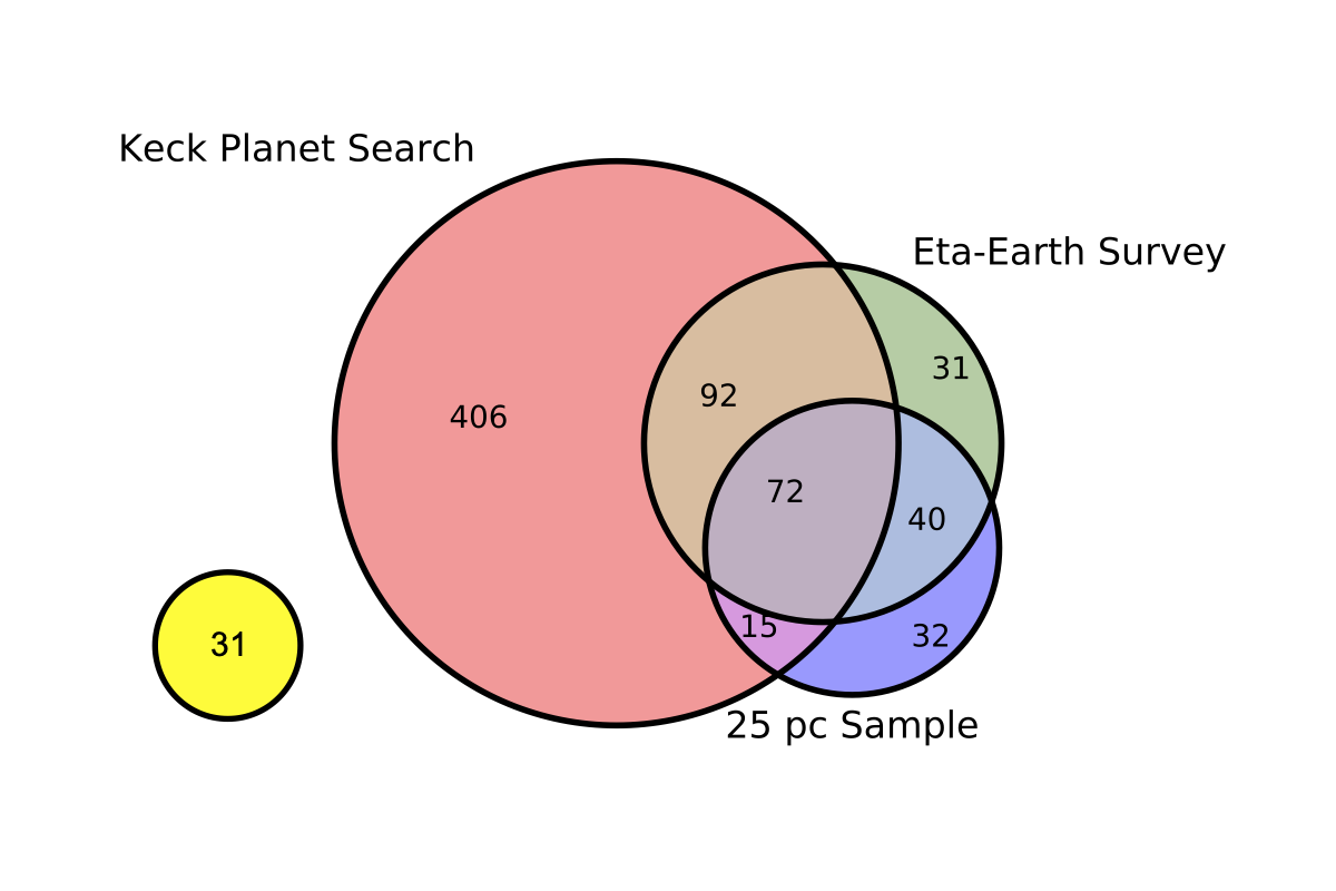
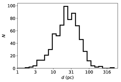
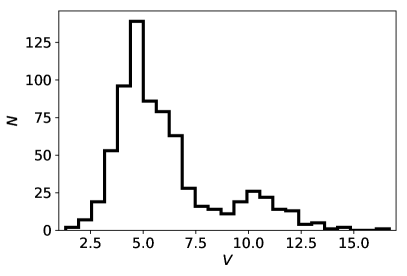
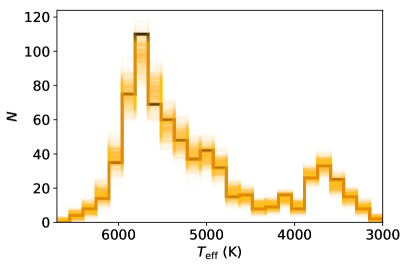
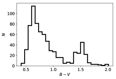
This selection process left us with nstars-legacynstars-legacy719 nstars-new135 [] stars. Figure 1 shows the entire CLS samples as a Venn diagram, illustrating the overlap of the Cumming et al. (2008) sample with the Eta-Earth (Howard et al., 2010b) and 25 pc northern hemisphere volume-limited (Hirsch et al., 2020) samples. The 25 pc sample includes 255 G and early K dwarfs with apparent $V$ magnitudes ranging from $V\approx 3$ to $V\approx 9$. These stars have a median temperature of 5360 K and a median mass of 0.86 $M_{\odot}$. The median number and duration of RV observations for this sample was 71 RVs spanning 21 yr, while the minimum number and duration of observations in the sample was 20 RVs spanning 3 yr. The architects of all three of these surveys designed them for planet occurrence studies. Therefore, they did not construct these catalogs by selecting on properties known to correlate or anticorrelate with planet occurrence. There are only 31 stars in the California Legacy Survey that do not belong to any of these three surveys but do still pass of our selection criteria. This survey has no hard constraints on distance, apparent magnitude, or color, as seen in Figure 4.

Figure 1: Venn diagram showing the overlap between the stars in the Keck Planet Search sample (Cumming et al., 2008), the Eta-Earth sample (Howard et al., 2010a), and a 25 pc northern hemisphere volume-limited survey (Hirsch et al. in prep). 31 stars in the California Legacy Survey do not belong to the union of these three surveys.

3 Observations

3.1 Keck-HIRES

HIRES (Vogt et al., 1994) has been in operation on the Keck I Telescope since 1994 and has been used to measure stellar RVs via the Doppler technique since 1996 (Cumming et al., 2008). This technique relies on measuring the Doppler shift of starlight relative to a reference spectrum of molecular iodine, which is at rest in the observatory frame (Butler et al., 1996). We consistently set up HIRES with the same wavelength format on the CCDs for each observation and followed other standard procedures of CPS Howard et al. (2010a). With the iodine technique, starlight passes through a glass cell of iodine gas heated to 50^∘ C, imprinting thousands of molecular absorption lines onto the stellar spectrum, which act as a wavelength reference. We also collected an iodine-free “template” spectrum for each star. This spectrum is naturally convolved with the instrumental point spread function (PSF) and is sampled at the resolving power of HIRES ($R$ = 55,000–86,000, depending on the width of the decker used). These spectra are deconvolved using PSF measurements from spectra of featureless, rapidly rotating B stars with the iodine cell in the light path. The final, deconvolved intrinsic stellar spectra serve as ingredients in a forward-modeling procedure from which we measure relative Doppler shifts of each iodine-in spectrum of a given star (Valenti et al., 1995). We also used this process to compute uncertainties on the Doppler shifts. The uncertainty for each measurement is the standard error on the mean of the RVs for 700 segments of each spectrum (each 2 Åwide) run through the Doppler pipeline. We distinguish between “pre-upgrade” RVs (1996–2004; $\sim$3 m s^-1 uncertainties) and “post-upgrade” RVs (2004–present; $\sim$1 m s^-1 uncertainties). In 2004, HIRES was upgraded with a new CCD and other optical improvements. We account in the time series modeling for different RVs zero points ($\gamma$) for data from the two different eras.

The RVs reported here stem from HIRES observations with a long history. The RVs from 1996 to 2004 are based on HIRES spectra acquired by the California & Carnegie Planet Search (CCPS) collaboration and were reported in Cumming et al. (2008). CCPS continued to observe these stars, but split into two separate collaborations: CPS and the Lick-Carnegie Exoplanet Survey (LCES). This paper principally reports results from 41,804 CPS and CCPS HIRES spectra that were obtained and analyzed by our team during 1996–2020. In addition, we have included RVs computed by our pipeline for 7530 spectra of CLS stars taken by LCES during 2008–2014. These HIRES spectra were acquired with the same instrumental setup as the CPS spectra and are publicly available in the Keck Observatory Archive. Butler et al. (2017) separately published RVs based on the same HIRES observations from CCPS, CPS, and LCES for the 1996–2014 time span. The LCES and CPS Doppler pipelines diverged in $\sim$2007. Tal-Or et al. (2019) uncovered the 2004 zero-point offset, which we model with two independent offsets. They also claimed two second-order systematics in the LCES 2017 dataset: a long-term drift of order $<$ 1 m s^-1, and a correlation between stellar RVs and time of night with respect to midnight. They estimated the long-term drift by averaging the zero points of three RV-quiet stars on each night, where possible. However, by our estimates, even the quietest stars exhibit 1–2 m s^-1jitter in HIRES time series. Averaging the zero points of three such stars will likely yield a scatter of 1 m s^-1across many nights. Additionally, they did not remove planet RV signals from their data before estimating the linear correlation between RV and time of night, and it is unclear how they derived the uncertainty in that correlation.

3.2 Automated Planet Finder

The APF-Levy spectrograph is a robotic telescope near the summit of Mt. Hamilton, designed to find and characterize exoplanets with high-cadence Doppler spectroscopy (Vogt et al., 2014; Radovan et al., 2014). The facility consists of a 2.4-m telescope and the Levy Spectrometer, which has been optimized for optical Doppler shift measurements. The Doppler pipeline that was developed for Keck-HIRES also extracts RV measurements from APF spectra. Most of the APF data in the California Legacy Survey was collected as part of the APF-50 Survey (Fulton, 2017), the stellar sample of which was drawn entirely from the Eta Earth sample. These two surveys have slightly different selection criteria. While both surveys have a distance cut $d<25$ pc and luminosity cut $M_{V}<3$, Eta-Earth cuts on apparent magnitude $V<11$, whereas APF-50 has $V<7$; Eta-Earth cuts on chromospheric activity $\mathrm{log}R^{\prime}_{\mathrm{HK}}<-4.7$, whereas APF-50 has $\mathrm{log}R^{\prime}_{\mathrm{HK}}<-4.95$; and Eta-Earth cuts on declination $>-30^{\circ}$, whereas APF-50 has declination $>-10^{\circ}$. These stricter cuts were made to ensure higher data quality for the high-cadence APF survey.

3.3 Lick-Hamilton

The Hamilton Spectrograph is a high-resolution echelle spectrometer, attached to the 3 m Shane telescope on Mt. Hamilton. Beginning in 1987, and ending in 2011 with a catastrophic iodine cell failure, the Lick Planet Search program (Fischer et al., 2014) monitored 387 bright FGKM dwarfs to search for and characterize giant exoplanets. This was one of the first surveys to produce precise RVs via Doppler spectroscopy with iodine cell calibration, and yielded RVs with precision in the range 3–10 m s^-1. The Lick Planet Search overlaps heavily with the Keck Planet Search and other CPS surveys, since these surveys drew from the same bright-star catalogs.

3.4 Activity Indices

For each HIRES and APF spectrum from which we measure radial velocities, we also measure the strength of emission in the cores of the Ca II H & K lines (S-values) following the techniques of Isaacson & Fischer (2010) and Robertson et al. (2014). There is a small, arbitrary offset between the HIRES and APF activity indices. We adopted uniform S-value uncertainties with values of 0.002 and 0.004 for HIRES and APF respectively. We provide activity indices along with our RV measurements. Missing values are the result of sky contamination and/or low SNR.

3.5 APT Photometry

We collected long-term photometric observations of the subset of our sample that were included in the APF-50 survey (Fulton, 2017), in order to search for evidence of rotation-induced stellar activity. We collected these measurements with Tennessee State University’s Automated Photometric Telescopes (APTs) at Fairborn Observatory as part of a long-term program to study stellar magnetic activity cycles (Lockwood et al., 2013). Most stars have photometric datasets spanning 15 – 23 yr. The APTs are equipped with photomultiplier tubes that measure the flux in the Stromgren $b$ and $y$ bands relative to three comparison stars. We combined the differential $b$ and $y$ measurements into a single $(b+y)/2$ “passband” then converted the differential magnitudes into a relative flux normalized to 1.0. The precision in relative flux is typically between 0.001 and 0.0015. Further details of the observing strategy and data reduction pipeline are available in Henry (1999); Eaton et al. (2003); Henry et al. (2013). We make the photometric data available as a machine-readable table.

3.6 Observational Statistics

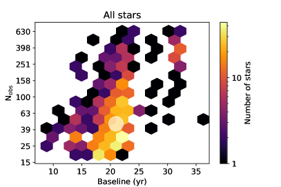
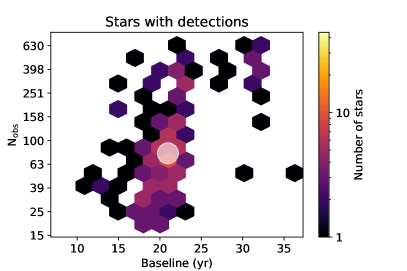
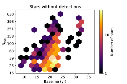
We examined the range of observing cadences and observational baselines within the CLS sample, to determine whether stars without known planets were observed with strategies that differed significantly from those for stars with known planets. Figure 2 shows the distribution of number of observations and observational baselines for three groups of stars: the entire sample, the stars around which we detected planets, and the star around which we did not detect planets. Each of these three samples has a median baseline of 21 yr. Stars with detected planet have a median of 74 observations, compared to 35 observations for stars without detected planets and 41 observations for the entire CLS sample. A factor of two in number of observations will have a small but measurable impact on planet detectability of a given data set – and therefore on its search completeness contours.

Figure 2: Distributions of observational baseline versus number of observations. The top panel shows these statistics for all stars in the CLS sample; the center panel shows stars around which we detect planets; the bottom panel shows stars around which we do not detect planets. Median baseline and number of observations for each sample are overplotted as translucent circles.

4 Stellar properties

We derived stellar properties for our sample by applying the SpecMatch (Petigura, 2015) and Isoclassify (Huber, 2017) software packages to the template Keck-HIRES spectra of our stars. Specmatch takes an optical stellar spectrum as input, and by interpolating over a grid of template spectra with known associated stellar properties, returns three spectral properties and uncertainties. For stars hotter than 4700 K, we interpolated over synthetic spectra to derive spectral parameters (Petigura, 2015). For stars below this threshold, we interpolated over real spectra of cool stars with well-characterized stellar properties, since synthetic spectral models are unreliable below this temperature (Yee et al., 2017).

Specmatch produces metallicity, effective temperature, and surface gravity when interpolating over synthetic spectra; it produces metallicity, effective temperature, and radius when interpolating over empirical spectra. Isoclassify takes effective temperature, metallicity, and surface gravity as spectral parameter inputs, and uses isochrone models and multinest Bayesian sampling (Buchner, 2016) to produce estimates and uncertainties of physical parameters, in particular stellar mass. For stars cooler than 4700 K, we passed Isoclassify a wide Gaussian input prior on surface gravity, since temperature and metallicity strongly constrain the masses of cool, main-sequence stars (Johnson et al., 2017).

Almost all stars in the California Legacy Survey have both Gaia-measured parallaxes (Gaia Collaboration et al., 2016, 2018; Lindegren et al., 2018) and apparent $K$-band magnitudes. For stars with both of these measurements available, we pass them and their uncertainties into Isoclassify as additional inputs, since taken together, they constrain stellar luminosity and therefore place tighter constraints on stellar mass. Isoclassify also returns more precise estimates of stellar radius when provided with parallax and apparent magnitude. With the inclusion of this luminosity constraint, the median precision of our stellar mass measurements is 3.6$\%$.

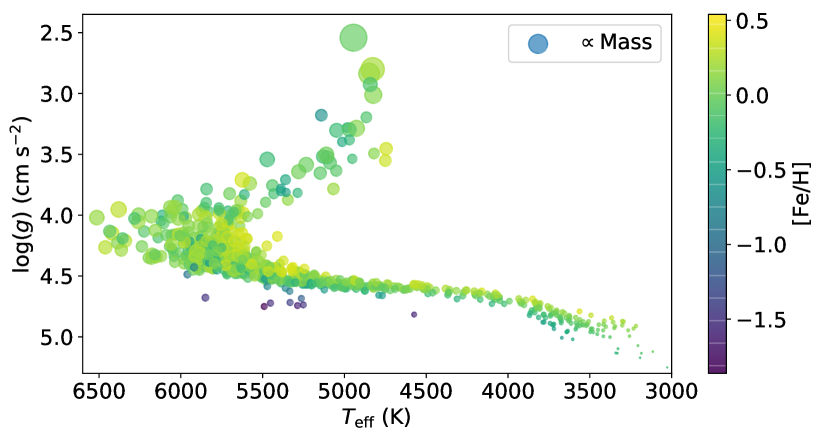
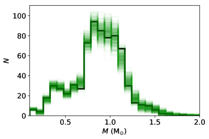
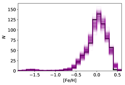
In Table 2 in Appendix B, we report stellar mass, radius, surface gravity, effective temperature, and metallicity for a subsection of the CLS sample. We make this table available for the entire sample in machine-readable format, with additional columns including $V$-band magnitude and Gaia parallax. Figure 3 is a visualization of these stellar properties, while Figure 4 shows individual histograms for mass, metallicity, and effective temperature, as well as for the following observational properties: parallax-inverse distance, $V$, and $B-V$.

Figure 3: Stellar property measurements of the California Legacy Survey, in effective temperature, surface gravity, and mass. The sample consists of stars spanning spectral types F, G, K, and M, some of which have evolved off of the main sequence. Most stars have metallicities within 0.4 dex of Solar metallicity, with the exception of a small handful of extremely metal-poor stars, which lie below the main sequence on this plot.

Figure 4: Stellar parameter distributions. The left column shows mass, metallicity, and effective temperature, while the right column shows parallax-inferred distance, $V$-band magnitude, and $B-V$ color. Black lines are histograms of the stellar parameter median values. For the left column, colored lines are 500 histograms per panel, with parameters redrawn from normal distributions with width equal to their individual measurement uncertainties. We left these redrawn parameter histograms out for the plots in the right column because distance, magnitude, and color have uncertainties that are smaller than the chosen bin size.

5 Planet Catalog Methods

5.1 Planet Search

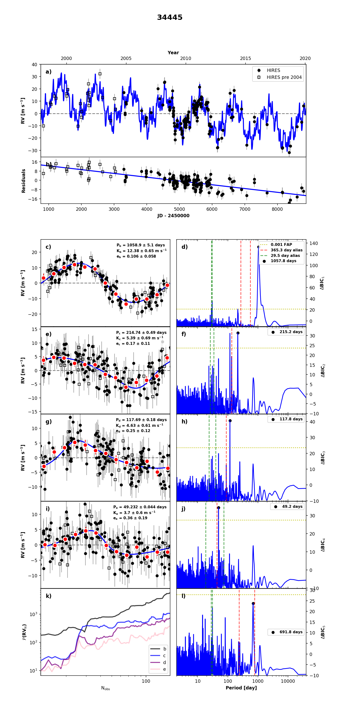
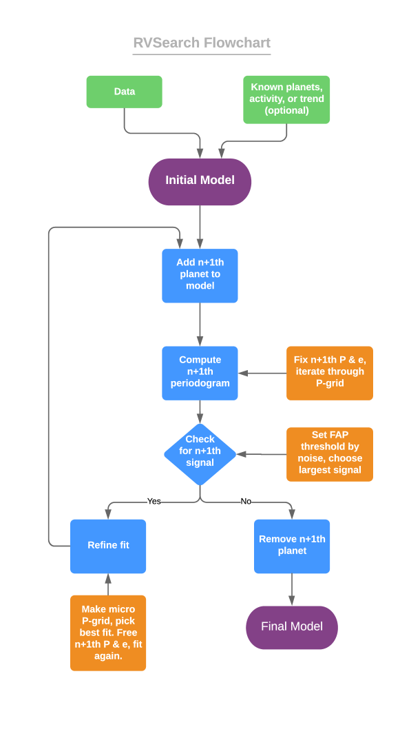
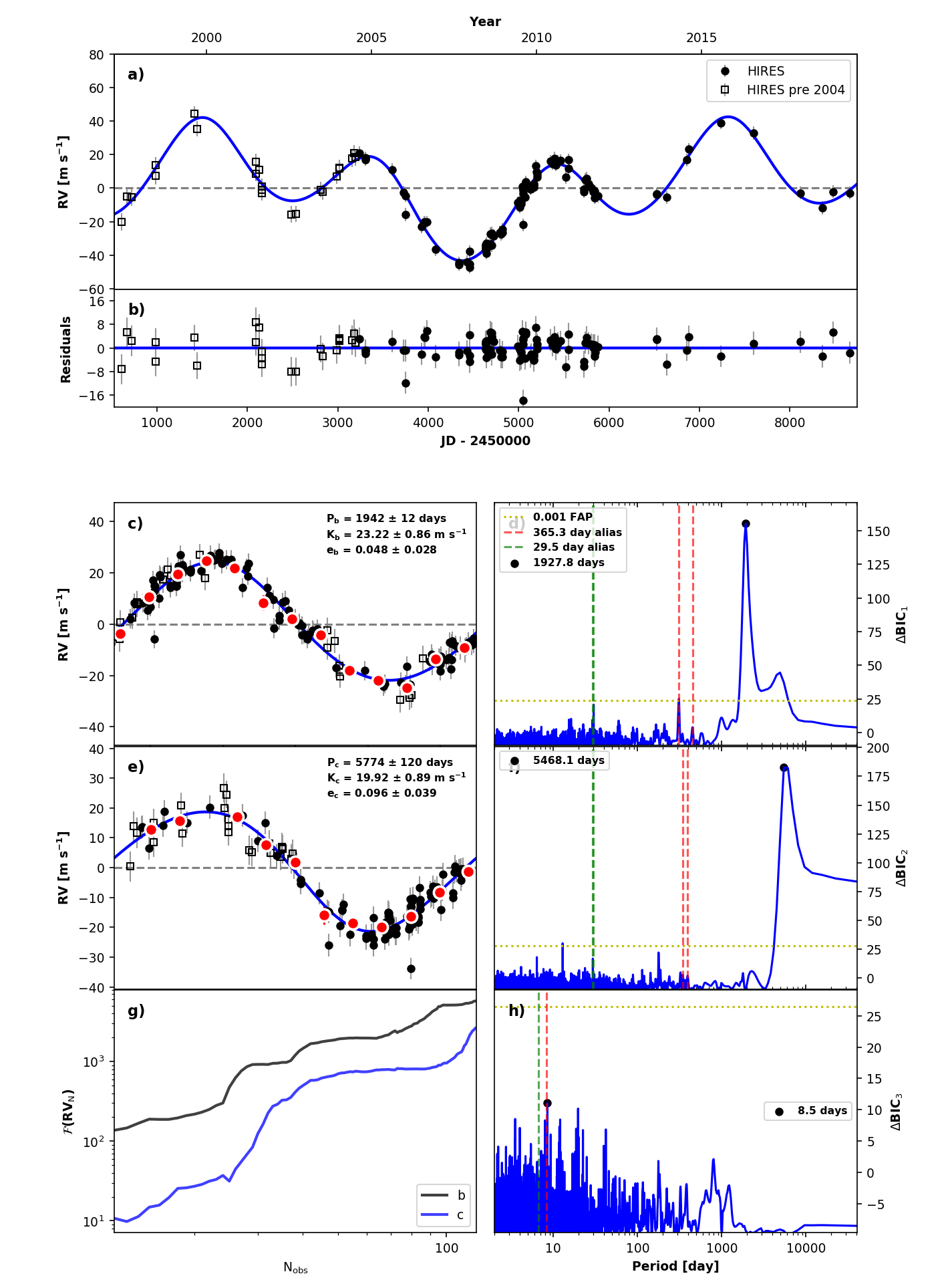
We developed an iterative approach to a search for periodic signals in RV data in order to generate the CLS planet catalog. We outline this algorithm, which we developed as the open-source Python package RVSearch and have made public alongside the publication of this paper. Figure 5 is a flowchart that lays out each step of the algorithm, and Figure 6 is a visualization of an example RVSearch output, where the top two panels show the final model, and each successive row shows an iterative search for each signal in the model. First, we provide an initial model, from which the iterative search begins. This initial model contains an RV data set, and a likelihood function. The natural logarithm of the latter is defined as

$$\textrm{ln}(\mathcal{L})=-\frac{1}{2}\sum_{i}\left[\frac{(v_{i}-m(t_{i})-\gamma_{D})^{2}}{\sigma_{i}^{2}}+\textrm{ln}(2\pi\sigma_{i}^{2})\right],\\$$ (1)

where $i$ is the measurement index, $v_{i}$ is the $i$th RV measurement, $\gamma_{D}$ is the offset of the instrumental dataset from which the $i$th measurement is drawn, and $\sigma_{i}^{2}$ is the quadrature sum of the instrumental error and the stellar jitter term of the $i$th measurement’s instrumental data set. Here, $m(t_{i})$ is the model RV at time $t_{i}$, defined as

$$m(t)=\sum_{n}\textrm{K}(t|K_{n},P_{n},e_{n},\omega_{n},t_{cn})+\dot{\gamma}(t-t_{0})+\ddot{\gamma}(t-t_{0})^{2},\\$$ (2)

where $n$ is a given Keplerian orbit in the model, $\textrm{K}(t|K,P,e,\omega,t_{c})$ is the Keplerian orbit RV signature at time $t$ given RV amplitude $K$, period $P$, eccentricity $e$, argument of periastron $\omega$, and time of inferior conjunction $t_{c}$, $\dot{\gamma}$ is a linear trend term, $\ddot{\gamma}$ is a quadratic trend term, and $t_{0}$ is a reference time, which we defined as the median time of observation.

We used RadVel (Fulton et al., 2018) to fit Keplerian orbits. The initial likelihood model contains either a one-planet Keplerian model with undefined orbital parameters, or a predefined model including trend/curvature terms and/or Keplerian terms associated with known orbital companions. We defaulted to performing a blind search starting with the undefined single-planet model, and we only supply a predefined model if there is evidence for a highly eccentric companion whose period is misidentified by our search algorithm. Several highly eccentric stellar binaries satisfy this criterion, as do two planets: HD 120066 b (Blunt et al., 2019), and HD 80606 b (Wittenmyer et al., 2007b).

Before beginning a blind search, RVSearch determines whether the data merits a trend with curvature, a linear trend, or no trend. It does this by fitting each of these three models to the data, then performing a goodness-of-fit test to decide which model is favored. We measured the Bayesian Information Criterion (BIC) for each of the three models, and computed the $\Delta\mathrm{BIC}$ between each model. RVSearch selects the linear model if it has $\Delta\mathrm{BIC}$ = 5 with respect to the flat model, and the quadratic model if it has $\Delta\mathrm{BIC}$ = 5 with respect to the linear model. We did not perform this test on datasets that contain eccentric companions with orbital periods greater than the data’s observational baseline, since such datasets would be better fit with a long-period Keplerian orbit than with linear and parabolic trends. The Bayesian information criterion is defined as

$$\textrm{BIC}=k\textrm{ln}(n_{\textrm{obs}})-2\textrm{ln}(\mathcal{L}),\\$$ (3)

where $n_{\textrm{obs}}$ is the number of observations, $k$ is the number of free model parameters, and $\textrm{ln}(\mathcal{L})$ is the log-likelihood of the model in question.

Once we provide an initial model, RVSearch defines an orbital period grid over which to search, with sampling such that the difference in frequency between adjacent grid points is $\frac{1}{2\pi\tau}$, where $\tau$ is the observational baseline. We chose this grid spacing in accordance with Horne & Baliunas (1986), who state that, in frequency space, a Lomb–Scargle periodogram has a minimum peak width of  $\frac{1}{2\pi\tau}$. For each dataset, we searched for periodicity between two days and five times the observational baseline. Searching out to five times the baseline only adds a few more points to the period grid, and it allows for the possibility of recovering highly eccentric, ultra-long-period planet candidates with best-fit orbital period.

The search algorithm then computes a goodness-of-fit periodogram by iterating through the period grid and fitting a sinusoid with a fixed period to the data. We measure goodness-of-fit as the $\Delta\mathrm{BIC}$ at each grid point between the best-fit, $n$+1-planet model with the given fixed period, and the $n$-planet fit to the data (this is the zero-planet model for the first planet search).

After constructing a $\Delta\mathrm{BIC}$ periodogram, the algorithm performs a linear fit to a log-scale histogram of the periodogram power values. The algorithm then extrapolates a $\Delta\mathrm{BIC}$ detection threshold corresponding to an empirical false-alarm probability of 0.1$\%$, meaning that, according to the power-law fit, only 0.1$\%$ of periodogram values are expected to fall beyond this threshold. This process follows the detection methodology outlined in Howard & Fulton (2016).

If a periodic signal exceeds this detection threshold, RVSearch refines the fit of the corresponding Keplerian orbit by performing a maximum a posteriori (MAP) fit with all model parameters free, including eccentricity, and records the BIC of that best-fit model. RVSearch includes two hard-bound priors, which constrain $K>0$ and $0<=e<1$. The algorithm then adds another planet to the RV model and conducts another grid search, leaving all parameters of the known Keplerian orbits free so that they might converge to a more optimal solution. In the case of the search for the second planet in a system, the goodness of fit is defined as the difference between the BIC of the best-fit one-planet model and the BIC of the two-planet model at each fixed period in the grid. RVSearch once again sets a detection threshold in the manner described above, and this iterative search continues until it returns a nondetection.

This iterative periodogram search is superior to a Lomb–Scargle residual subtraction search in two key ways. First, this process fits for the instrument-specific parameters of each dataset, stellar jitter and RV-offset, as free parameters throughout the search. Second, by leaving the known model parameters free while searching for each successive planet, we allow the solutions for the already discovered planets to reach better max-likelihood solutions that only become evident with the inclusion of another planet in the model.

Note that our search and model comparison process is not Bayesian; we do not use priors to inform our model selection, and we do not sample posteriors, beyond a grid search in period space, until we settle upon a final model. We use the BIC as our model comparison metric because it incorporates the number of free parameters as a penalty on more complex models, which, in our case, corresponds to models with additional planets.

We make RVSearch publicly available alongside this paper via a GitHub repository. See the RVSearch website for installation and use instructions.

Figure 5: Search algorithm flowchart.

Figure 6: Example RVSearch summary plot, for the known two-planet system HIP 109388. Panel a) shows the total model plotted over the radial velocity time series, while panel b) shows the model residuals. Each successive row shows a phase-folded signal discovered by RVSearch on the left, and the associated periodogram on the right. The final row shows the running periodograms of each signal, generated with Lomb–Scargle power, on the left, and the final periodogram on the right.

5.2 Search Completeness

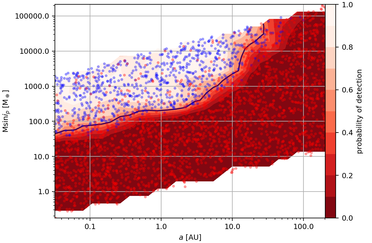
We characterized the search completeness of each individual dataset, and of the entire survey, by running injection-recovery tests. Once RVSearch completed an iterative search of a dataset, it injected synthetic planets into the data and ran one more search iteration to determine whether it recovers these synthetic planets in that particular dataset. We ran 3000 injection tests for each star. We drew the injected planet period and $M\sin{i}$ from log-uniform distributions, and drew eccentricity from the beta distribution described in Kipping (2013), which was fit to a population of RV-observed planets.

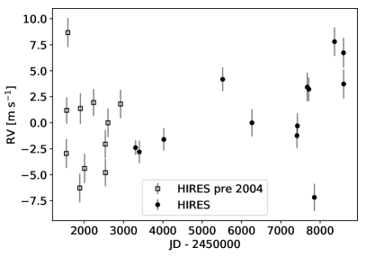
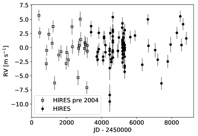
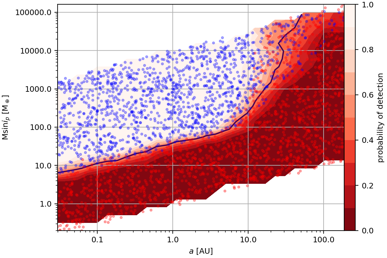
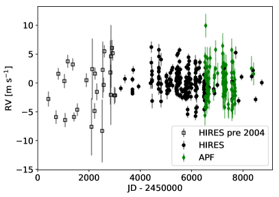
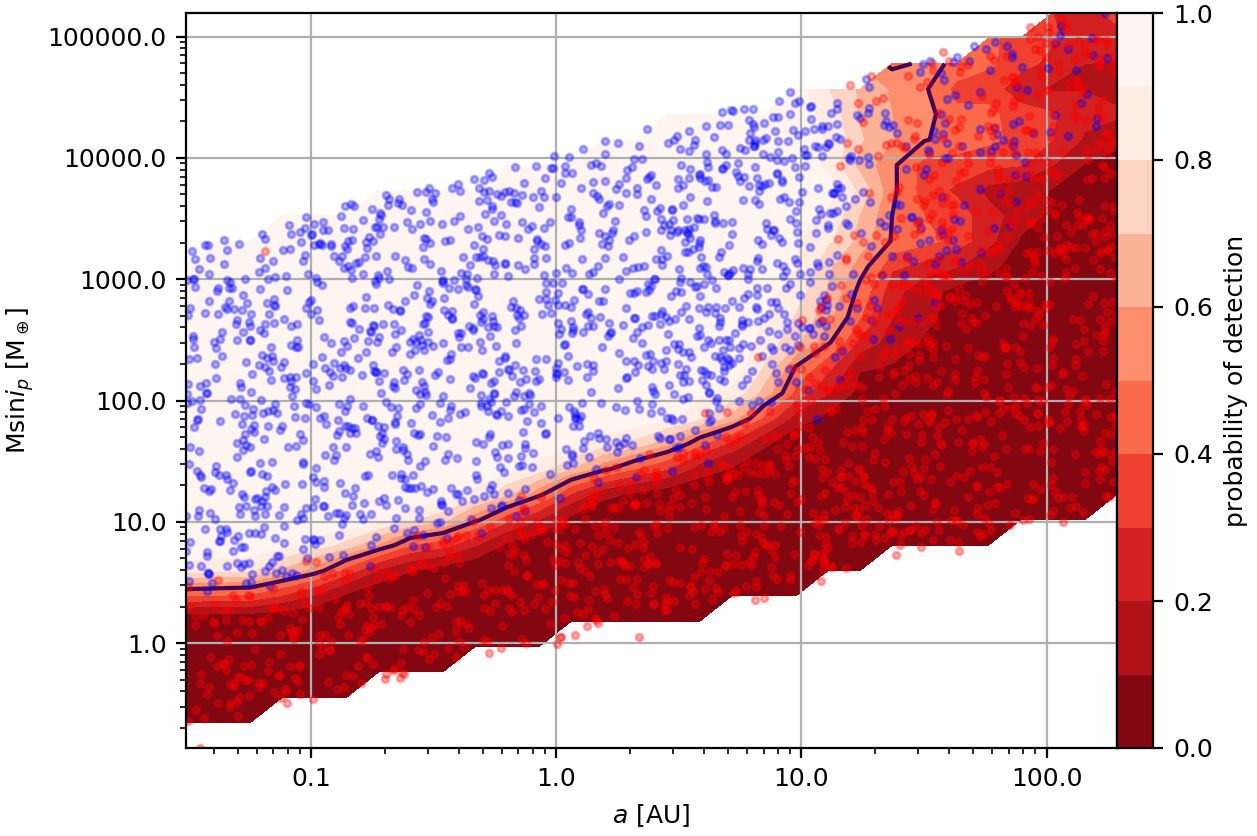
We used the results of these injection tests to compute search completeness for each individual dataset, and report constant $M\sin{i}$ / $a$ contours of detection probability. Figure 7 shows examples of these contours and the corresponding RVs for three different stars, all early G-type: one with 25 observations, one with 94, and one with 372. We make the 10th, 50th, and 90th percentile completeness contours for each individual star available in machine-readable format.

Figure 7: RVs and completeness contours for three datasets with similar baselines, median measurement errors, and stellar jitter. The left column plots RVs with respect to time, while the right column plots injected signals in the $M\sin{i}$ and $a$ plane, where blue dots are recovered injections and red dots are not. The right column also shows detection probability contours, with 50$\%$ plotted as a solid black line. From top to bottom, we show RVs and contours for HD 44420, for which we have 24 RVs; HD 97343, for which we have 94 RVs; and HD 12051, for which we have 372 RVs.

5.3 Model posteriors

Once RVSearch returned max-likelihood estimates of the orbital model parameters for a given dataset, we sampled the model posterior using affine-invariant sampling, implemented via emcee and RadVel (Foreman-Mackey et al., 2013; Fulton et al., 2018). We sampled using the orbital parameter basis $\{$ $\mathrm{log}P\ K\ t_{c}\ \sqrt{e}\mathrm{sin}\omega\ \sqrt{e}\mathrm{cos}\omega$ $\}$. We placed uniform priors on all fitting parameters, with hard bounds such that $K>0$ and $0\leq e<1$. We fit in $\mathrm{log}P$ space to efficiently sample orbits with periods longer than our observational baseline, and in $\sqrt{e}\mathrm{sin}\omega$ and $\sqrt{e}\mathrm{cos}\omega$ to minimize bias toward higher eccentricities (Lucy & Sweeney, 1971). We reported parameter estimates and uncertainties as the median and $\pm$1$\sigma$ intervals.

If a dataset is so poorly constrained by a Keplerian model that emcee’s affine-invariant sampler cannot efficiently sample the posterior distribution, we instead used a rejection sampling algorithm to estimate the posterior. In these cases, we used TheJoker (Price-Whelan et al., 2017), a modified MCMC algorithm designed to sample Keplerian orbital fits to sparse radial velocity measurements. We chose a flat prior on $\mathrm{log}P$, with a minimum at the observing baseline and a maximum at twenty times the observing baseline. We drew orbital eccentricity from a beta prior weighted toward zero, as modeled in Kipping (2013), in order to downweight orbits with arbitrarily high eccentricity, which can be viable fits to sparse or otherwise underconstraining RV data sets.

5.4 False-positive vetting

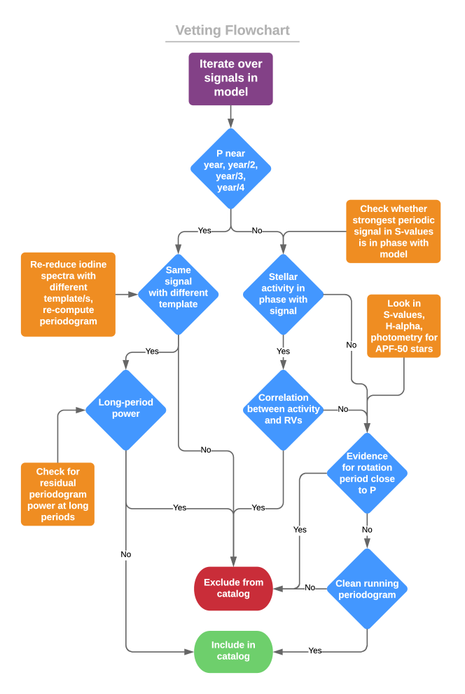
We performed a series of tests to vet each planet candidate discovered by our search pipeline. The following subsections each detail one test we perform to rule out one way in which a signal might be a false-positive. We also represent this process with a flowchart in Figure 9, and include a table of all false-positive signals recovered by RVSearch in Table 6.

5.4.1 Stellar activity, magnetic/long-period

Many main-sequence stars, particularly F- and G-type, have magnetic activity cycles on timescales of several to tens of years. These fluctuations in activity can cause changes in the core depths of stellar Calcium H & K lines, which manifest as apparent RV shifts (Isaacson & Fischer, 2010). To evaluate whether stellar activity may be the cause of a signal recovered by our search pipeline, we measure the linear correlation between the RV signature of that signal and a measured stellar activity metric–in our case, S-values. We computed S-values for both post-upgrade HIRES and APF data by measuring the core flux of Calcium H & K lines.

If we found a periodic signal in the S-value data that has a similar period and phase similar to one of the Keplerian terms in our RV model, we searched for correlations between our RV model and S-values. If we found one periodic signal in an RV dataset, we measured its correlation with stellar activity simply as the linear correlations between the RVs of each instrument and their associated S-values. If we found multiple periodic signals, then for each signal, we subtracted the associated RV models of all other signals from the data, and measured the correlations between these residuals and the S-values. A significant linear correlation between a signal’s RV residuals and the associated S-values does not necessarily mean that this signal is caused by stellar activity, even when these signals also have the same period and phase, but we took it as sufficient evidence to remove such signals from our catalog of confirmed planets.

It is important to note that our approach to vetting our planet candidates is systematic but not exhaustive, particularly with respect to stellar activity. One might use activity metrics beyond S-values and photometry, such as H$\alpha$ line modulation. Furthermore, there are more sophisticated ways to deal with activity than searching for linear correlations with RVs. For instance, one might actively model stellar activity during the search process, using a Gaussian Process (Haywood et al., 2014) or some other correlated noise model. Such techniques might improve the accuracy of our planet candidate parameters and catalog selection, but require case-by-case analysis for each stellar system, as activity modeling is sometimes unwarranted or even counterproductive, e.g., for low-activity stars or confirmed planets that have periods similar to their host star’s activity cycle. We chose to perform uniform, after-the-fact vetting for our catalog, and invite others to perform more sophisticated modeling for individual systems of interest.

5.4.2 Stellar activity, rotation/short-period

We only detected planet candidates that are low-amplitude and short-period enough to possibly be stellar rotation false positives in sustained, high-cadence datasets. Almost all CLS datasets that satisfy this criteria were collected as part of the APF-50 survey. We collected APT photometry of all APF-50 stars, which we can use to search for evidence of stellar rotation with moving-average smoothing and periodogram analysis. If we find strong evidence for rotation in APT photometry, or spectral S-value measurements, we discount planet candidates with periods close to the apparent rotation timescale or its harmonics.

5.4.3 Yearly alias

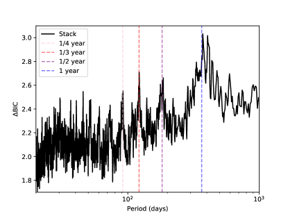
When we find a signal with a period of a year or an integer fraction of a year, we investigate whether it is an alias of long-period power, or a systematic that is correlated with the barycentric velocity at the time of observation or Doppler fitting parameters. We do this by recomputing the associated RVs using a different template observation. When another template observation was unavailable, we were able to take one using Keck-HIRES during collaborator observing nights. Templates taken in poor observing conditions or when barycentric velocity with respect to the observed star is high can produce systematic errors in the Doppler code. If a search of this new dataset returns a nondetection, or detection at a significantly different period, we conclude that this signal is an alias. Figure 8 shows the presence of yearly alias power in our survey, seen in a stack of the the final nondetection periodograms of all CLS stars.

Figure 8: Stack of all final nondetection periodograms in the CLS planet search, linearly interpolated to the same period grid. A broad peak around 1 year is evident, as well as narrow peaks at 1/2-year, 1/3-year, and 1/4-year.

Figure 9: Candidate vetting flowchart.

6 Planet and Stellar/Substellar Companion Catalog

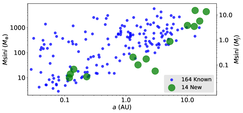
We present orbital solutions for the known planets, substellar companions, and stellar binaries that RVSearch has recovered in the California Legacy Survey. As mentioned in Section 5.1, where appropriate, we modeled long-period companions with linear or parabolic trends. We included in the appendix portions of the tables associated with each class of object: one for planets, one for stellar and substellar companions that are best modeled by Keplerian orbits, and one for stars with linear or parabolic RV trends. We also present 14 newly confirmed or significantly revised exoplanets and substellar companions. We list them and their orbital parameters in Table 1, and include individual notes on each system in Appendix A. Figure 10 shows all recovered planets in our survey, and distinguishes between known planets and new discoveries.

Figure 10: Scatterplot of best-fit $M\sin{i}$ and semi-major axis values for planets in the CLS catalog. Blue dots represent known planets, while green circles represent newly discovered planets and planets with significantly revised orbits.

Table 1: Discovered or Revised Planets and Substellar Companions

CPS Name	Lit. Name	$M\sin{i}$ [$M_{\textrm{J}}$] ($M_{\oplus}$)	$a$ [AU]	$e$	$P$ [d]	$t_{c}-2450000$ [d]	$\omega$
HD 107148 c	HD 107148 c	$0.0626^{+0.0097}_{-0.0098}$ ($19.9^{+3.1}_{-3.1}$)	$0.1406^{+0.0018}_{-0.0018}$	$0.34^{+0.13}_{-0.16}$	$18.3267^{+0.0022}_{-0.0024}$	$5203.4^{+1.4}_{-1.3}$	$-0.78^{+0.67}_{-0.42}$
HD 136925 b	HD 136925 b	$0.84^{+0.078}_{-0.074}$ ($267^{+25}_{-24}$)	$5.13^{+0.12}_{-0.11}$	$0.103^{+0.094}_{-0.070}$	$4540^{+160}_{-140}$	$-310^{+280}_{-330}$	$0.42^{+0.69}_{-1.30}$
HD 141004 b	HIP 77257 b	$0.0428^{+0.0047}_{-0.0045}$ ($13.6^{+1.5}_{-1.4}$)	$0.1238^{+0.002}_{-0.002}$	$0.16^{+0.11}_{-0.10}$	$15.5083^{+0.0016}_{-0.0018}$	$6704.33^{+0.55}_{-0.49}$	$0.34^{+0.55}_{-0.74}$
HD 145675 c	14 Her c	$5.8^{+1.4}_{-1.0}$	$16.4^{+9.3}_{-4.3}$	$0.45^{+0.17}_{-0.15}$	$25000^{+24000}_{-9200}$	$4680^{+440}_{-310}$	$-0.13^{+0.14}_{-0.18}$
HD 156668 b	HD 156668 b	$0.0991^{+0.0079}_{-0.0077}$ ($31.5^{+2.5}_{-2.5}$)	$1.57^{+0.017}_{-0.017}$	$0.089^{+0.084}_{-0.061}$	$811.3^{+5.2}_{-5.3}$	$5890^{+25}_{-19}$	$-0.19^{+0.92}_{-0.74}$
HD 164922 e	HD 164922 e	$0.0331^{+0.0031}_{-0.0031}$ ($10.52^{+0.99}_{-0.97}$)	$0.2292^{+0.0026}_{-0.0027}$	$0.086^{+0.083}_{-0.060}$	$41.763^{+0.012}_{-0.012}$	$5256.6^{+1.2}_{-1.0}$	$-0.3^{+1.30}_{-0.87}$
HD 168009 b	HIP 89474 b	$0.03^{+0.0038}_{-0.0037}$ ($9.5^{+1.2}_{-1.2}$)	$0.1192^{+0.0017}_{-0.0018}$	$0.121^{+0.110}_{-0.082}$	$15.1479^{+0.0035}_{-0.0037}$	$5201.56^{+0.82}_{-0.77}$	$0.23^{+0.8}_{-1.1}$
HD 213472 b	HD 213472 b	$3.48^{+1.10}_{-0.59}$	$13.0^{+5.7}_{-2.6}$	$0.53^{+0.120}_{-0.085}$	$16700^{+12000}_{-4800}$	$9580^{+190}_{-160}$	$0.65^{+0.24}_{-0.25}$
HD 24040 c	HD 24040 c	$0.201^{+0.027}_{-0.027}$ ($63.9^{+8.6}_{-8.6}$)	$1.3^{+0.021}_{-0.021}$	$0.11^{+0.120}_{-0.079}$	$515.4^{+2.2}_{-2.5}$	$4984^{+19}_{-17}$	$-0.3^{+1.30}_{-0.87}$
HD 26161 b	HD 26161 b	$13.5^{+8.5}_{-3.7}$	$20.4^{+7.9}_{-4.9}$	$0.82^{+0.061}_{-0.050}$	$32000^{+21000}_{-10000}$	$10540^{+450}_{-280}$	$-0.07^{+0.13}_{-0.12}$
HD 3765 b	HIP 3206 b	$0.173^{+0.014}_{-0.013}$ ($54.8^{+4.3}_{-4.2}$)	$2.108^{+0.032}_{-0.033}$	$0.298^{+0.078}_{-0.071}$	$1211^{+15}_{-16}$	$5607^{+52}_{-54}$	$-1.1^{+2.60}_{-0.32}$
HD 66428 c	HD 66428 c	$27^{+22}_{-17}$	$23.0^{+19.0}_{-7.6}$	$0.32^{+0.23}_{-0.16}$	$39000^{+56000}_{-18000}$	$-4100^{+4600}_{-4500}$	$0.5^{+0.65}_{-1.40}$
HD 68988 c	HD 68988 c	$15.0^{+2.8}_{-1.5}$	$13.2^{+5.3}_{-2.0}$	$0.45^{+0.130}_{-0.081}$	$16100^{+11000}_{-3500}$	$1660^{+110}_{-180}$	$-0.13^{+0.037}_{-0.043}$
HD 95735 c	GJ 411 c	$0.0568^{+0.0091}_{-0.0083}$ ($18.0^{+2.9}_{-2.6}$)	$3.1^{+0.13}_{-0.11}$	$0.14^{+0.160}_{-0.095}$	$3190^{+200}_{-170}$	$7440^{+150}_{-150}$	$0.1^{+1.1}_{-1.3}$

7 Discussion

Through the use of high-cadence APF observations and long-baseline HIRES observations, we have expanded the population of known exoplanets along the current mass and semi-major axis boundary of detectability, as seen in Figure 10. We recovered 43 planets with $M\sin{i}$ $<$ 30 $M_{\oplus}$ , including four new discoveries within 1 AU. In a future paper in the California Legacy Survey series, we will leverage the decades-long-baseline datasets in which these planets were discovered, in order to constrain the probability that a host of a small planet also hosts an outer companion, as explored in Bryan et al. (2019) and Zhu & Wu (2018). We will also directly place a lower limit on the conditional occurrence of inner small planets given the presence of an outer gas giant.

In addition to expanding the population of small planets with measured $M\sin{i}$ , we discovered or revised the orbits of ten planets with orbital separations greater than 1 AU, six of them beyond 4 AU. We represent the model posteriors for the coldest of these planets in Figure 11, and show a gallery of some of their orbits in Figure 12. These discoveries include two new detections with incomplete orbits, HD 213472 b and HD 26161 b. Details are provided in Appendices A.3 and A.14. Using HIRES to extend the observational baseline of our survey by another decade will tighten our $M\sin{i}$ and orbital parameter constraints for these planets, and may reveal more cold companions beyond 10 AU.

In a future paper in the CLS series, we will use our sample of long-period planets and completeness contours to measure the mass–period planet occurrence distribution out to 10 AU, extending beyond the Keck Planet Search’s limit of 5 AU (Cumming et al., 2008) and the 9 AU limit of Wittenmyer et al. (2020). This will provide novel constraints on planet occurrence beyond the water ice line, resolve the discrepancy between the results of Fernandes et al. (2019) and those of Wittenmyer et al. (2020), and provide new insight into planet formation across protoplanetary disks.

Figure 11: Contours (1- and 2-$\sigma$) of $M\sin{i}$ and semi-major axes for planets in the CLS sample whose semi-major axis posteriors extend beyond 10 AU. Contours for HD 26161 b have hard cutoffs due to sparsity below 7 $M_{\textrm{J}}$ and 12 AU; these limits come from the data’s baseline and RV increase to date.

Figure 12: Orbit gallery for six of the coldest companions in our survey. We plot RV data and Keplerian model versus year, and subtract off the model signatures of inner companions and stellar activity. We did not include UMa 47 d, seen in Figure 11, in this plot, because its detection relied on early Lick-Hamilton RVs, and we wanted to showcase HIRES RV measurements from the past twenty-four years.

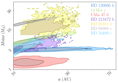
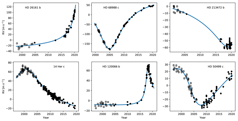
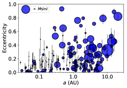
Figure 13 is a visualization of the eccentricities of all planets in the California Legacy Survey. In future work, we will quantify the eccentricity distribution of gas giants in our sample and its dependence on planet mass and multiplicity, as well as the eccentricity distributions of brown dwarfs and other substellar companions, in order to clarify possible formation pathways. We will extend the wide-orbit population comparisons of Bowler et al. (2020) to our sample of planets and brown dwarfs within 20 AU of their hosts. We will also explore the eccentricity distribution of gas giants beyond 7 AU. As Figures 12 and 13 show, all planets recovered beyond 7 AU are eccentric with significance $e>2\sigma_{e}$. This may be a selection effect, as the median baseline of observations in our sample is 21 yr, which corresponds to a semi-major axis of 7.6 AU for a planet orbiting a solar-mass star. It is possible that planets with orbital periods beyond our observational baselines are more easily detectable if they are eccentric. We can use injection-recovery tests to determine whether there is a detection bias toward eccentric planets beyond observational baselines. If this phenomenon is not a selection effect, it might imply that most giant planets beyond 7 AU have undergone a scattering event or otherwise been excited to high eccentricity. Taken together, these studies will leverage this decades-long observational undertaking to provide new insights into planet formation and evolution.

Figure 13: $M\sin{i}$ , $a$, and eccentricity of the CLS sample. Eccentricity is plotted in medians and 68$\%$ confidence intervals, while scatter size is proportional to $M\sin{i}$ posterior mode.

In our appendices, we have included individual notes on each planet discovery reported in this paper; complete tables of recovered planets, Keplerian-resolved stellar binaries, and substellar companions in the California Legacy Survey; signals that RVSearch recovered and we determined to be false-positives; linear and parabolic RV trends; and excerpts from the stellar sample and RV dataset, which are available in their entirety in machine-readable format.

Appendix A Individual Discoveries and Revised Orbits

A.1 HD 3765

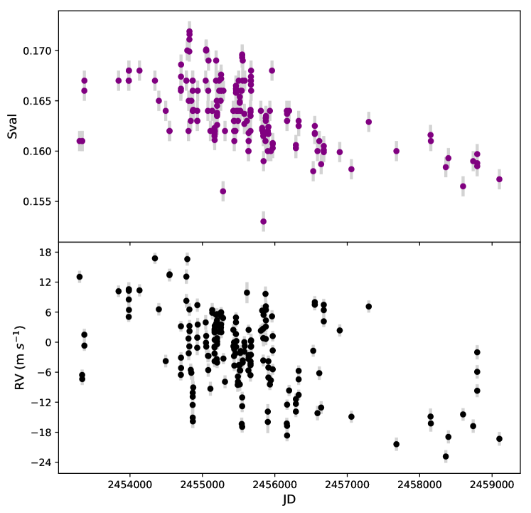
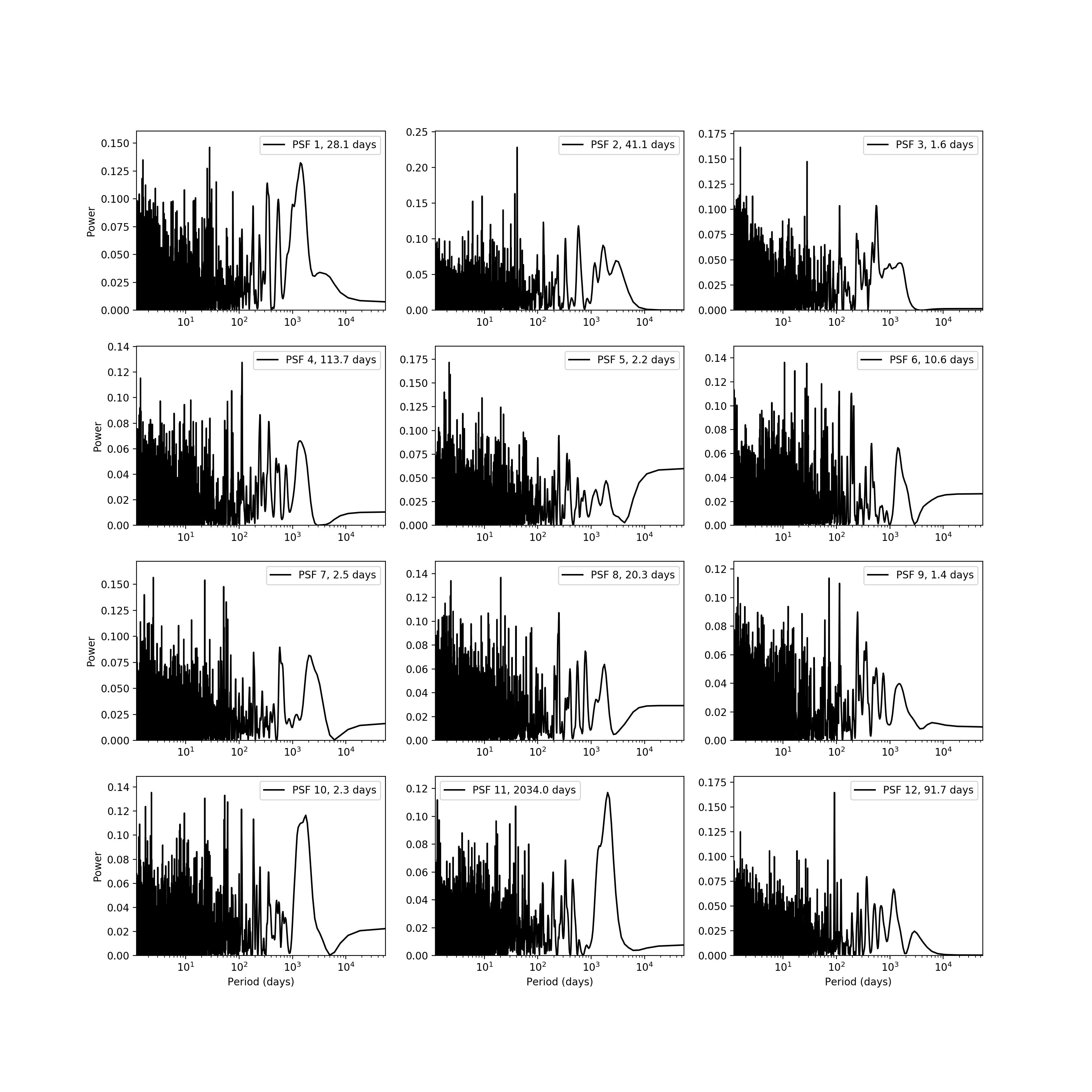
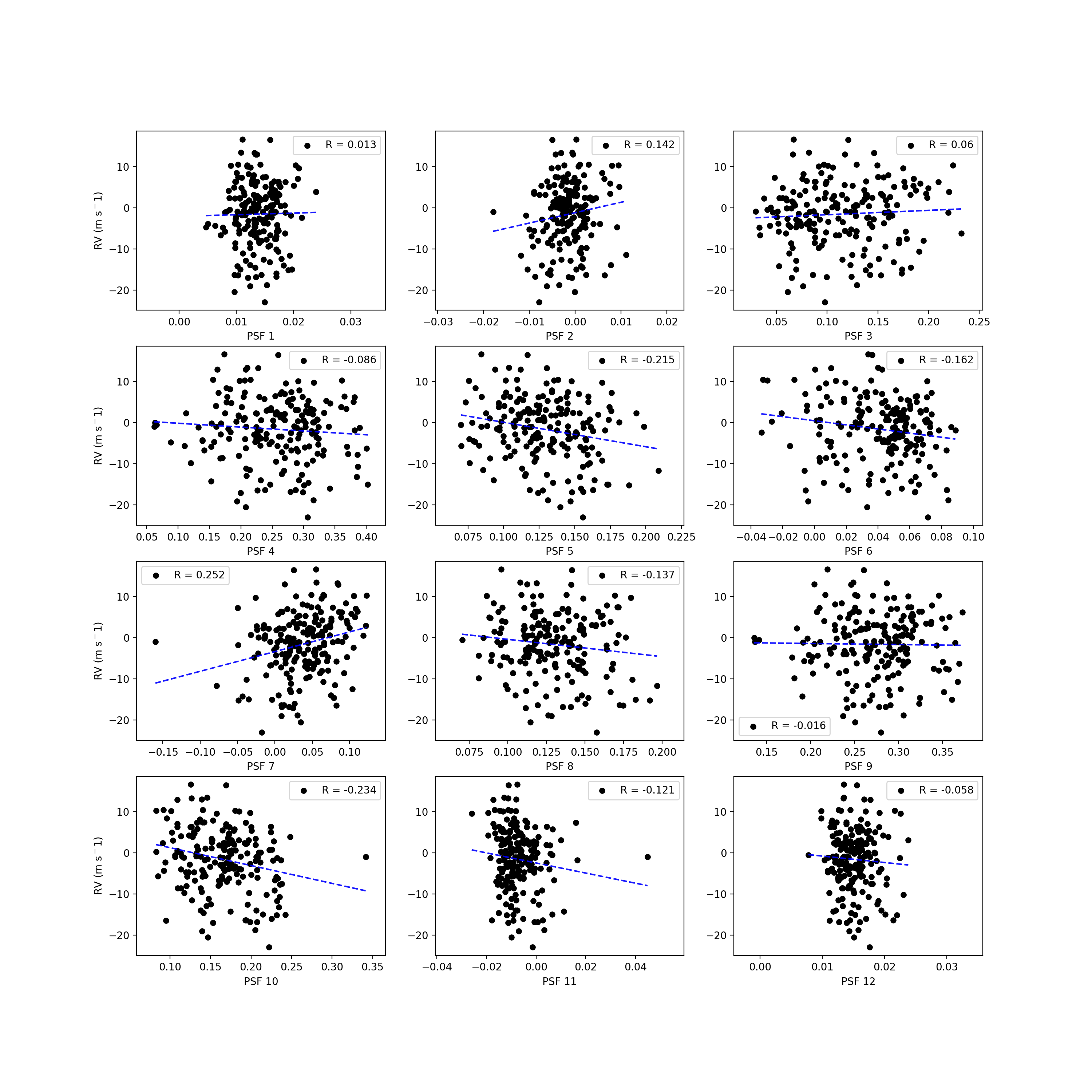
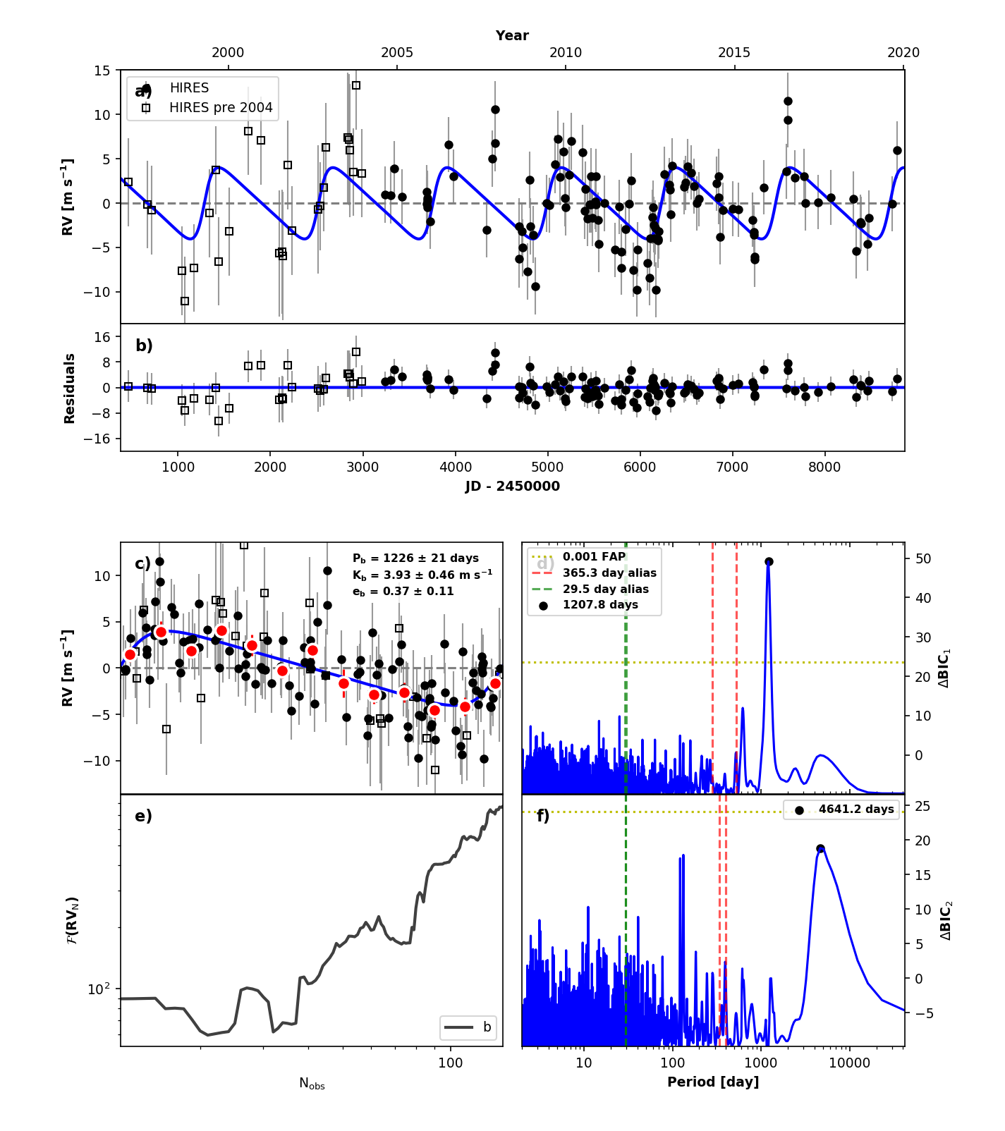
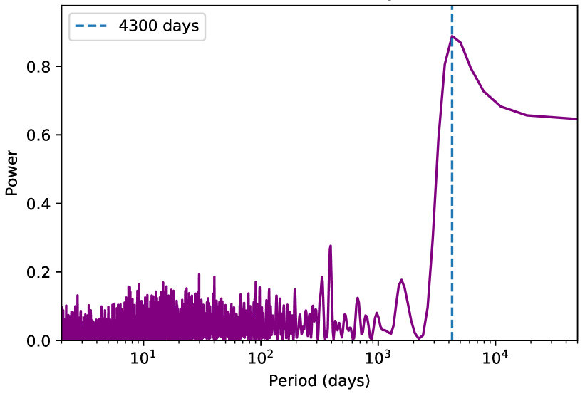
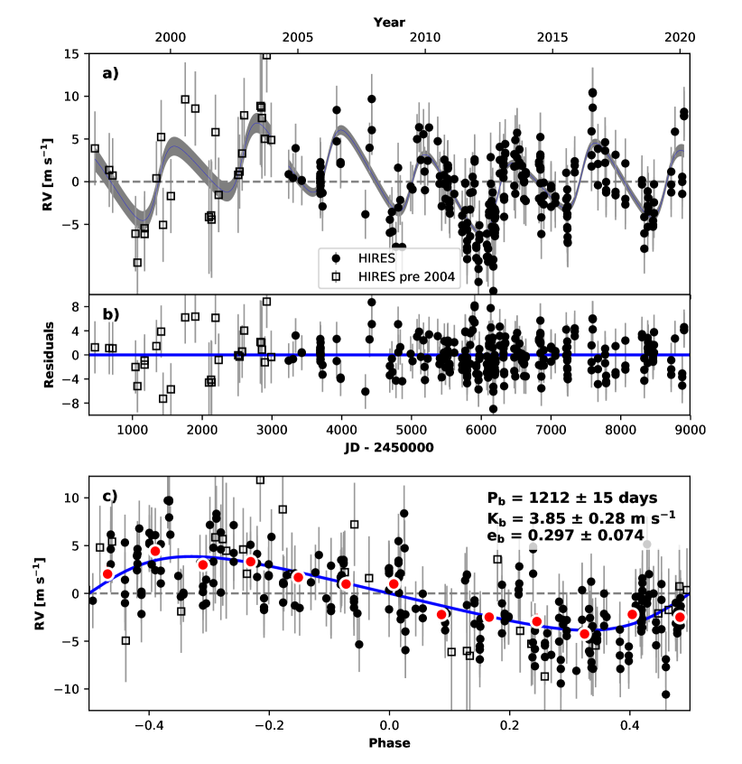
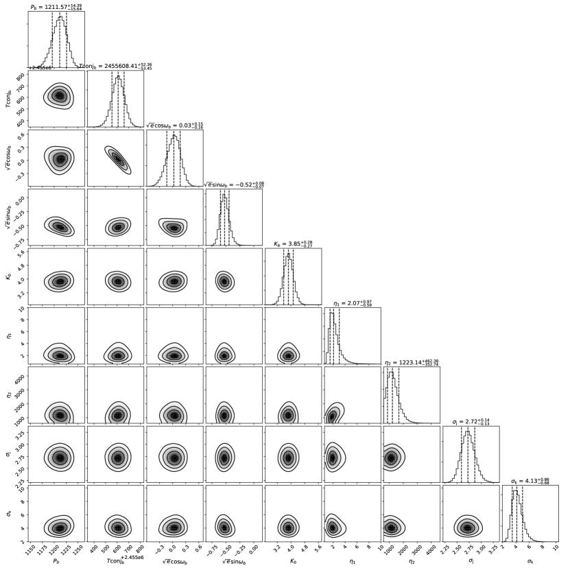
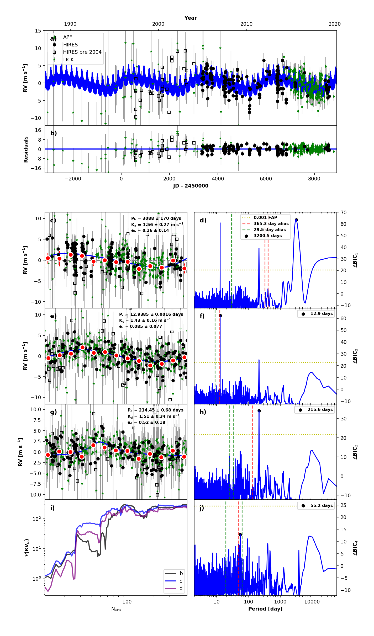
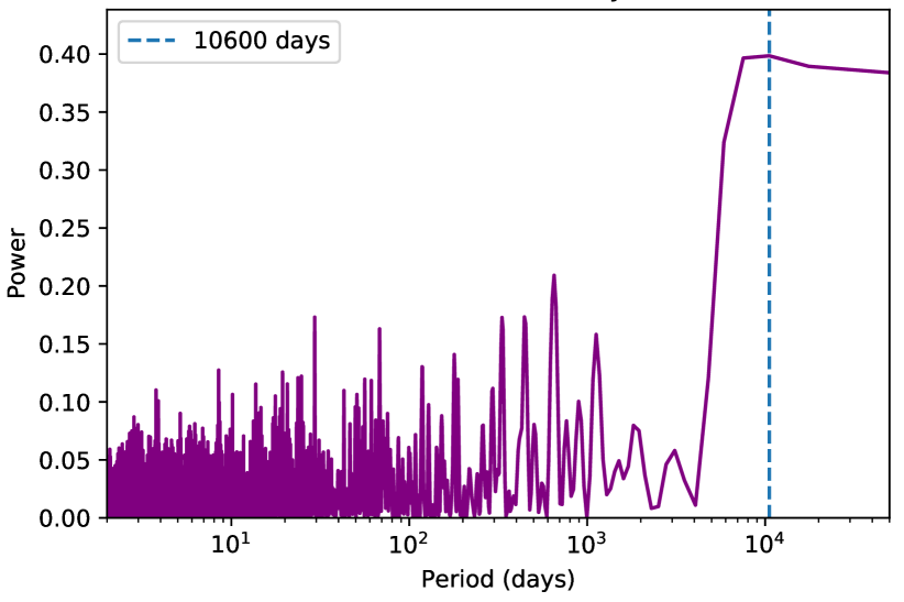
HD 3765 is a K2 dwarf at a distance of 17.9 pc (Gaia Collaboration et al., 2018). Figure 14 shows the RVSearch results for this star. We recovered a signal with a period of 3.36 yr. Table 1 reports all planet parameters. There is significant periodicity in the S-value time series, but concentrated around a period of 12 yr. Furthermore, we find no correlation between the RVs and S-values. Figure 15 shows a Lomb–Scargle periodogram of the S-value time series. Thus, we label this signal as a confirmed planet, with $M\sin{i}$ = $0.173\pm 0.014$ $M_{\textrm{J}}$ and $a=2.108\pm 0.033$ AU. The magnetic activity cycle is too weak for RVSearch to recover, but is evident in the best-fit RV residuals. We used RadVel to model this activity cycle with a squared-exponential Gaussian process, and report MCMC-generated posteriors for both orbital and Gaussian process parameters in Figure 16 and Figure 17.

Figure 14: RVSearch summary plot for HD 3765. See Figure 6 for plot description.

Figure 15: Lomb-Scargle periodogram of HIRES S-values for HD 3765. Significant power at and beyond 4,300 days.

Figure 16: RadVel model orbital plot for HD 3765, including a Gaussian process with a squared-exponential kernel. The grey shaded curve represents the 68$\%$ interval for the Gaussian process RV signature.

Figure 17: Orbital and Gaussian process parameter posteriors for HD 3765. $\eta_{1}$ is the GP amplitude, while $\eta_{2}$ is the GP exponential decay timescale.

A.2 HD 24040

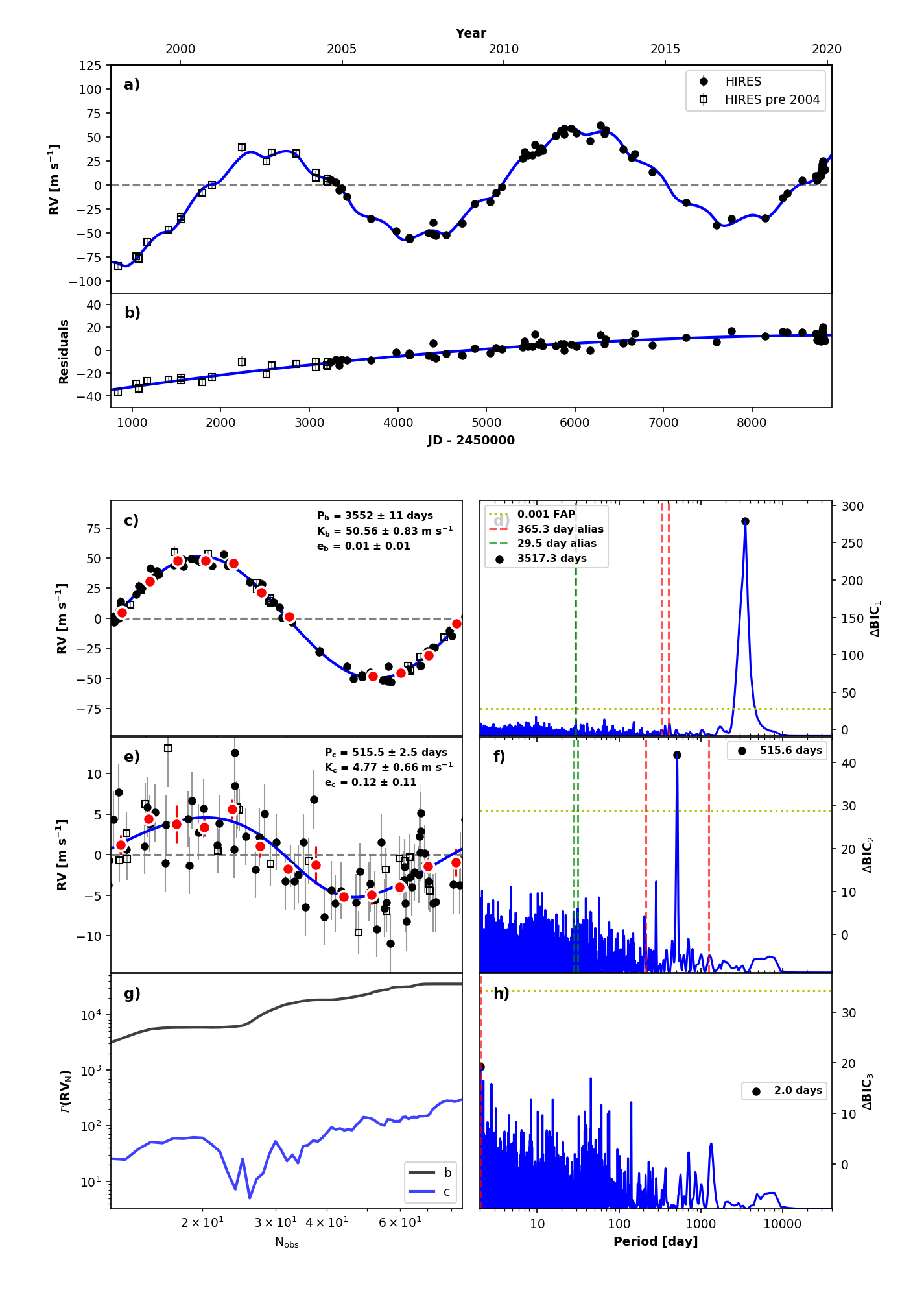
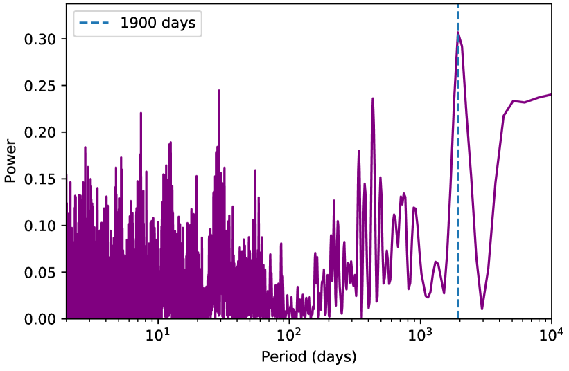
HD 24040 is a G1 dwarf at a distance of 46.7 pc. Figure 18 shows the RVSearch results for this star. It hosts a known gas giant (Wright et al., 2007; Feng et al., 2015) with a semi-major axis that we measured as $a=4.72\pm 0.18$ AU, an orbital period of $9.53\pm 10^{-4}$ yr, and a minimum mass $M\sin{i}$ = $4.09\pm 0.22$ $M_{\textrm{J}}$. We have extended the observational baseline of our HIRES measurements to 21.7 yr, constrained the long-term trend and curvature of the RVs, and discovered a new exoplanet, a sub-Saturn ($M\sin{i}$ = $0.201\pm 0.027$ $M_{\textrm{J}}$) on a 1.4 yr orbit ($a=1.30\pm 0.021$ AU) that is consistent with circular. The S-values are uncorrelated with the the RVs of both planet signals, after removing the long-term trend. Figure 19 shows a Lomb–Scargle periodogram of the S-value time series. Table 1 reports all planet parameters.

In addition to the newly detected sub-Saturn, we further constrained the known linear trend in the RVs and found evidence for a curvature term as well. RVSearch detected a curvature term with model preference $\Delta\mathrm{BIC}$$>$ 10 over a purely linear trend. We measured the linear trend to be $0.00581\pm 0.00044$ m s^-1 d^-1, and the curvature to be $-6.6\times 10^{-7}\pm 1.2\times 10^{-7}$ m s^-1 d^-2, a 5.5$\sigma$ detection. The trend and curvature parameters are slightly correlated in the posterior, but neither is correlated with any of the Keplerian orbital parameters in the model. Therefore, we kept the curvature term that RVSearch selected in our model. This long-term trend is low-amplitude enough that it may be caused by another planet in the system, orbiting beyond 30 AU. Gaia astrometry or another two decades of RVs may provide further constraints on this object.

Figure 18: RVSearch summary plot for HD 24040. See Figure 6 for plot description.

Figure 19: Lomb-Scargle periodogram of HIRES S-values for HD 24040. No periods show power that is statistically significant.

A.3 HD 26161

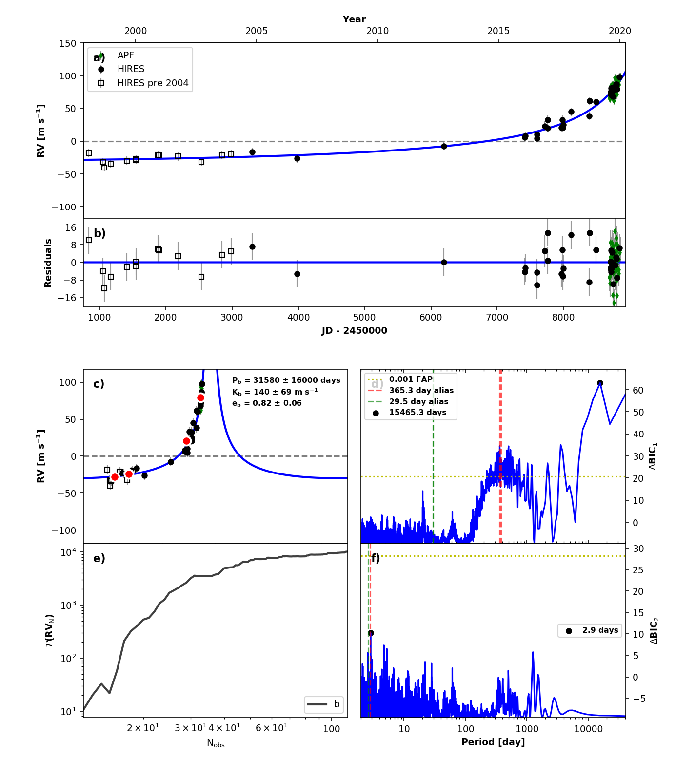
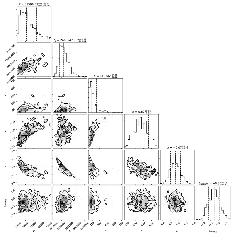
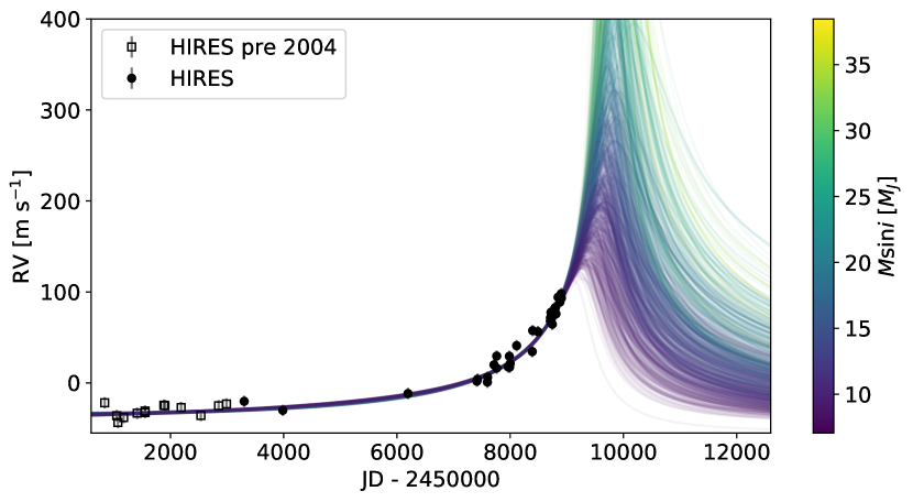
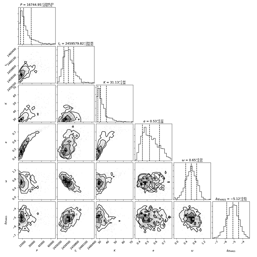
HD 26161 is a G0 dwarf located at a distance of 50.0 pc. Figure 20 shows the RVSearch results for this star. Our RVs are consistent with a long-period, eccentric companion, and RVSearch detected this long-period signal. Due to the sparseness of the data and the fractional orbital coverage, traditional MCMC methods fail to return a well-sampled model posterior. Since the data underconstrains our model, we used TheJoker to sample the posterior, which is consistent with an extremely long-period gas giant with minimum mass $M\sin{i}$ = $13.5\mathrm{\begin{subarray}{c}+8.5\\ -3.7\end{subarray}}$ $M_{\textrm{J}}$, semi-major axis $a=20.4\mathrm{\begin{subarray}{c}+7.9\\ -4.9\end{subarray}}$ AU, and eccentricity $e=0.82\mathrm{\begin{subarray}{c}+0.06\\ -0.05\end{subarray}}$. Table 1 reports current estimates of all orbital parameters, and Figure 21 shows their posterior distributions. A Keplerian model is significantly preferred over a quadratic trend, with $\Delta\mathrm{BIC}$$>$ 15.

The Simbad stellar catalog designates HD 26161 as a stellar multiple. We used Gaia to identify a binary companion with similar parallax and within 60 arcseconds. This companion has an effective temperature identified from Gaia colors of 4053 K, and a projected separation of 562 AU. A stellar companion that is currently separated from its primary by more than 560 AU could not cause a change in RV of 100 m s^-1over 4 yr. This curve is far more likely caused by an inner planetary or substellar companion approaching periastron.

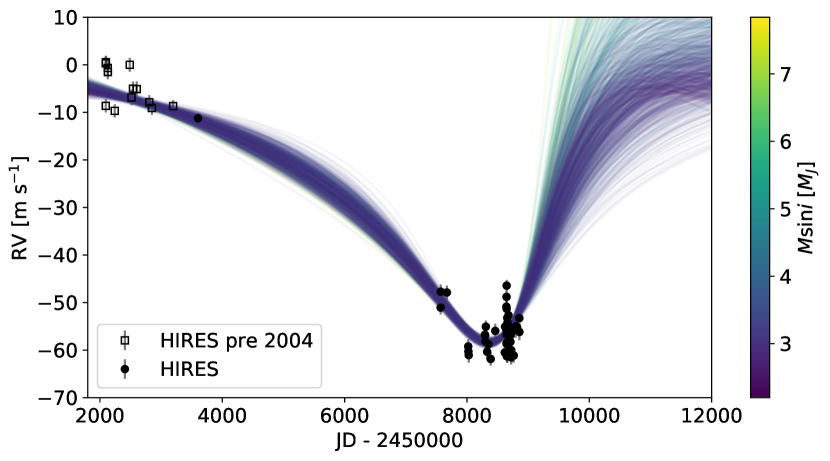
Figure 22 shows a sample of possible orbits for HD 26161 b, drawn from our rejection sampling posteriors and projected over the next decade. We will continue to monitor HD 26161 with HIRES at moderate cadence, and have begun observing this star with APF. As we gather more data during the approach to periastron, we can tighten our constraints on the minimum mass, eccentricity, and orbital separation of HD 26161 b.

Figure 20: RVSearch summary plot for HD 26161. See Figure 6 for plot description.

Figure 21: Rejection sampling posterior for HD 26161.

Figure 22: Possible orbits for HD 26161 b. RV curves are drawn from the rejection sampling posterior generated with TheJoker. The color of each orbit drawn from the posterior scales with $M\sin{i}$ .

A.4 HD 66428

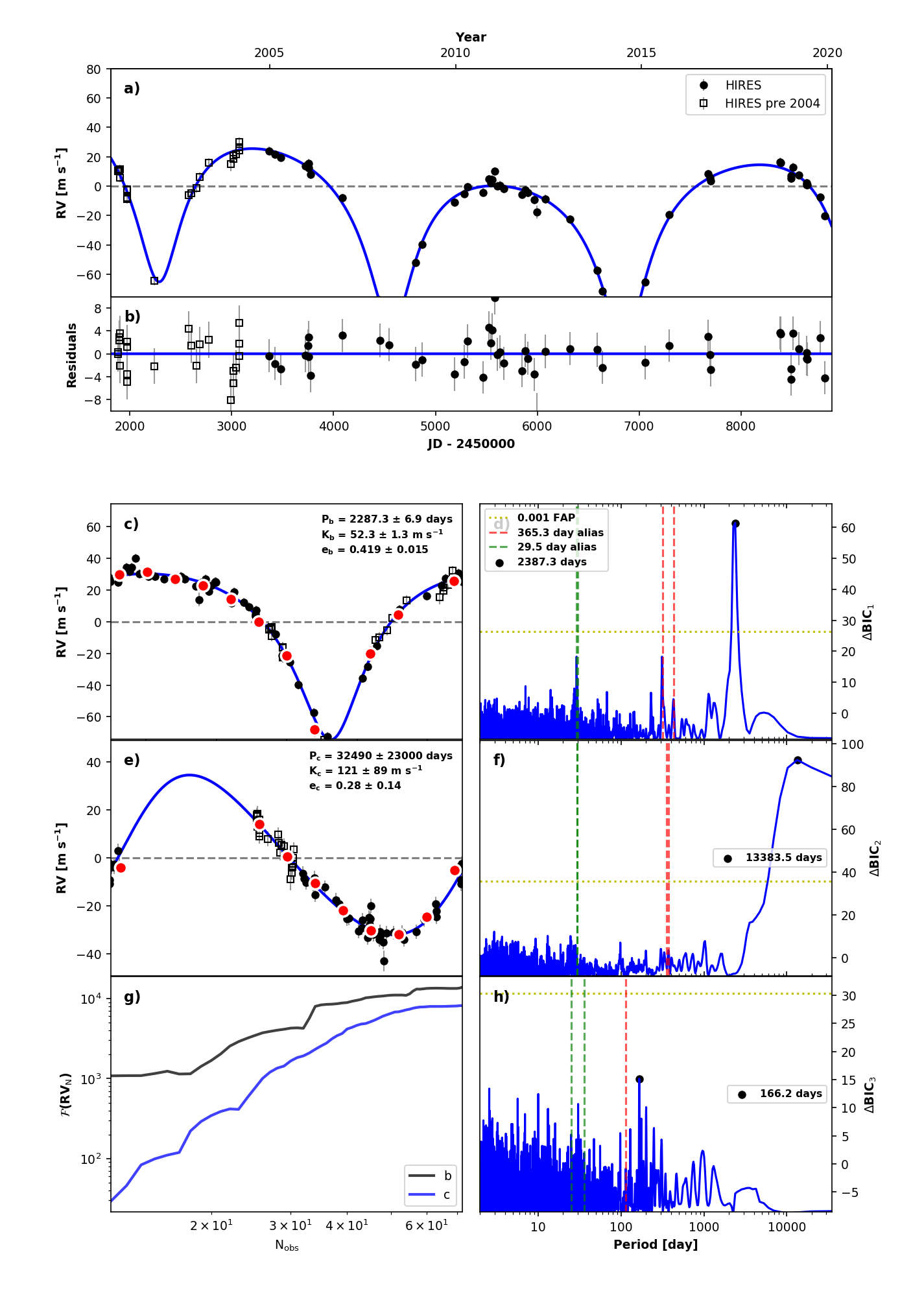
HD 66428 is a G8 dwarf found at a distance of 53.4 pc. Figure 23 shows the RVSearch results for this star. This system has one well-constrained cold Jupiter (Butler et al., 2006b) and an outer companion candidate first characterized in Bryan et al. (2016) as a linear trend. With four more years of HIRES data, we now see curvature in the RVs and a clear detection in RVSearch, and can place constraints on this outer candidate’s orbit with a Keplerian model. The Keplerian orbit for the outer candidate is preferred to a parabolic trend with $\Delta\mathrm{BIC}$$>$ 30. A maximum likelihood fit gives an orbital period of $P=36.4$ yr. However, since we have only observed a partially resolved orbit so far, the orbit posterior in period space is wide and asymmetric. MCMC sampling produces $P=88\mathrm{\begin{subarray}{c}+153\\ -49\end{subarray}}$ yr. Table 1 reports current estimates of all orbital parameters.

The model parameters are $M\sin{i}$ = $27\mathrm{\begin{subarray}{c}+22\\ -17\end{subarray}}$ $M_{\textrm{J}}$, $a=23.0\mathrm{\begin{subarray}{c}+19.0\\ -7.6\end{subarray}}$ AU, and $e=0.31\mathrm{\begin{subarray}{c}+0.13\\ -0.13\end{subarray}}$. This orbital companion could be a massive gas giant or a low-mass star, if we only consider constraints from RV modeling. However, Bryan et al. (2016) used NIRC2 Adaptive-Optics images to place upper bounds on the mass and semi-major axis of an outer companion, at a time when it only presented as a linear trend in HIRES RVs. They found an upper bound of $\approx$100 $M_{\textrm{J}}$ on mass, not just $M\sin{i}$, and an upper bound of $\approx$150 AU on $a$. We will continue to monitor this star with HIRES to further constrain the mass and orbit of HD 66428 c.

Figure 23: RVSearch summary plot for HD 66428. See Figure 6 for plot description.

A.5 HD 68988

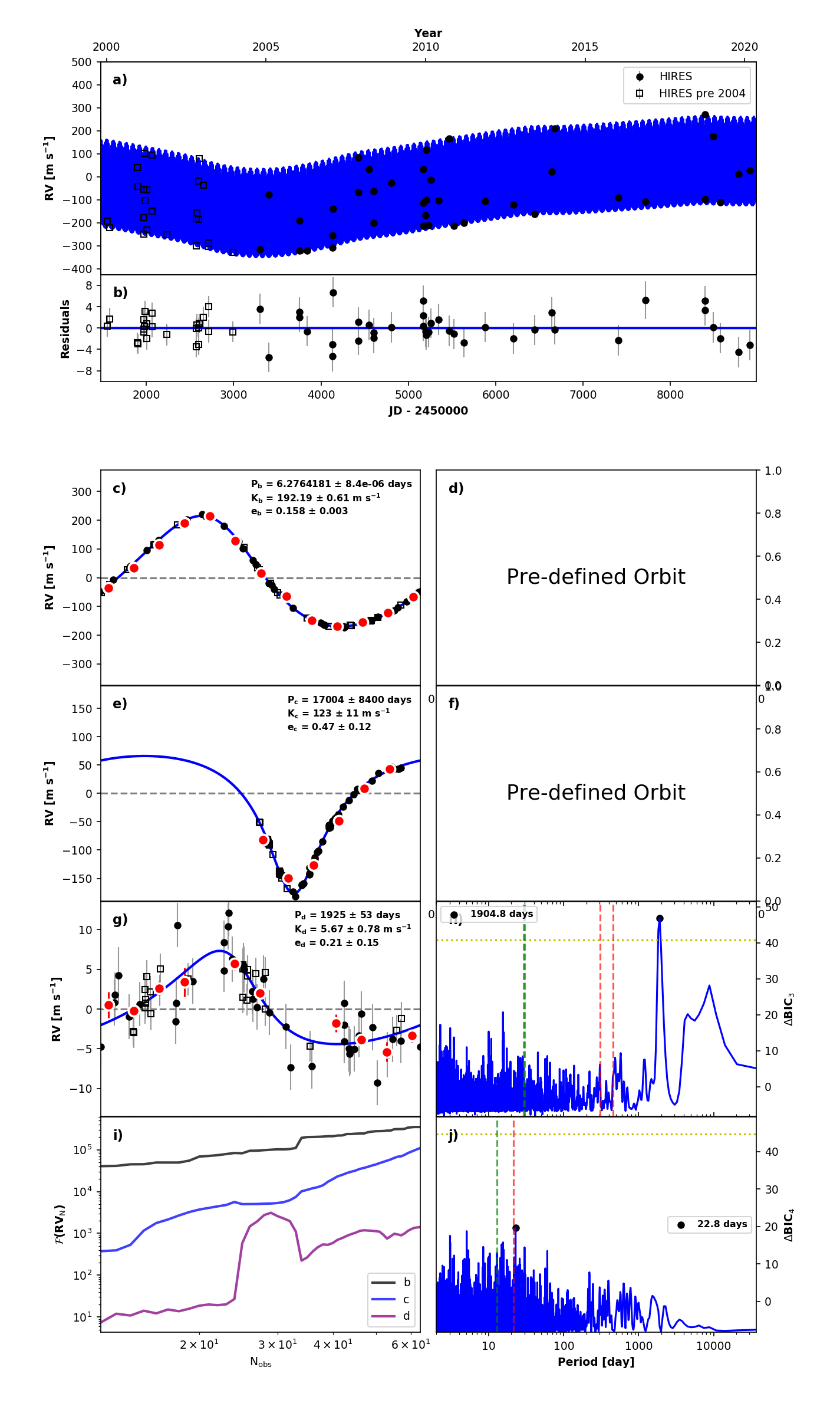
HD 68988 is a G0 dwarf found at a distance of 61 pc. Figure 24 shows the RVSearch results for this star. This system has one well-constrained hot Jupiter (Vogt et al., 2002) and an outer companion candidate that was first characterized in Bryan et al. (2016) as a partially resolved Keplerian orbit. With four more years of HIRES data, we can place tighter constraints on this outer candidate’s orbit. A maximum likelihood fit gives an orbital period of 49.2 yr. However, since we have only observed a partially resolved orbit so far, the orbit posterior is wide and asymmetric in period space. MCMC sampling produces $P=61\mathrm{\begin{subarray}{c}+28\\ -20\end{subarray}}$ yr. The model parameters are $M\sin{i}$ = $17.6\mathrm{\begin{subarray}{c}+2.4\\ -2.5\end{subarray}}$ $M_{\textrm{J}}$, $a=16.5\mathrm{\begin{subarray}{c}+4.8\\ -3.8\end{subarray}}$ AU, and $e=0.53\mathrm{\begin{subarray}{c}+0.13\\ -0.09\end{subarray}}$. Table 1 reports all companion parameters.

RVSearch detects a third periodic signal, with $P$ = 1900 days, that has the same period and phase as the peak period in the S-value time series. This signal also has a low RV amplitude,  6 m s^-1. Therefore, we designated this signal as a false-positive corresponding to stellar activity.

Figure 24: RVSearch summary plot for HD 68988. See Figure 6 for plot description.

A.6 HD 95735

HD 95735 (GJ 411) is an M2 dwarf found at a distance of 2.55 pc. Figure 25 shows the RVSearch results for this star. This system has one known short-period super-Earth, with $M\sin{i}$ = 3.53 $M_{\oplus}$ and an orbital period of 12.9 days. Our detection of this planet was driven by high-cadence APF data. This planet was first reported by Díaz et al. (2019), who also noted long-period power in their SOPHIE RV data, but they did not have a sufficiently long baseline or the activity metrics necessary to determine the origin of this power. With our HIRES post-upgrade and APF observations, we have an observational baseline of 14 yr, allowing us to confirm this long-period signal as a planet with $M\sin{i}$ = $24.7\pm 3.6$ $M_{\oplus}$ and an orbital period $P=8.46$ yr. Table 1 reports all planet parameters. Since GJ 411 is a cool M dwarf, the Lick-Hamilton and HIRES pre-upgrade data are not reliable, because those detectors are not sufficiently high-resolution to capture a cool M dwarf’s dense spectral lines (Fischer et al., 2014).

There is a long-period trend in the HIRES S-value time series, with significant power at and beyond 25 yr, but no significant power near the orbital period of the outer candidate. Therefore, we included this candidate in our catalog as a new planet candidate, to be verified and constrained with several more years of HIRES observations.

RVSearch also recovered a highly eccentric, 216 day signal, but this signal correlates with APF systematics. Therefore, we labeled it as a false positive. This systematic remained when we applied RVSearch only to the HIRES post-upgrade and APF data and left out the problematic pre-upgrade and Lick data.

Figure 25: RVSearch summary plot for HD 95735. See Figure 6 for plot description.

Figure 26: Lomb-Scargle periodogram of HIRES S-values for HD 95735. There is evidence for an activity cycle longer than 10,000 days, but no significant power near the period of our 3,000-day planet candidate.

A.7 HD 107148

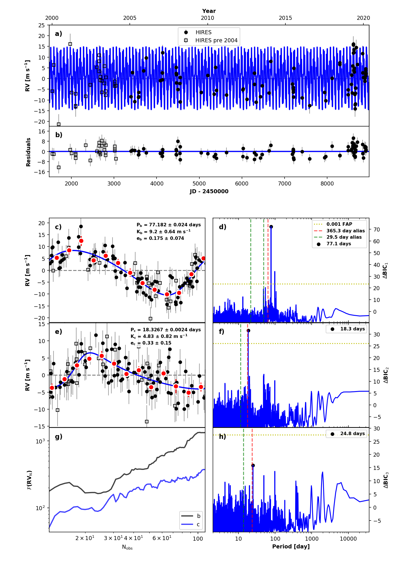
HD 107148 is a G5 dwarf at a distance of 49.5 pc. Figure 27 shows the RVSearch results for this star. Butler et al. (2006b) reported a planet with a period of 44 days. They reported periodicity at 77 days, but determined that this was an alias of the 44 day signal. The 77 day signal is significantly stronger in our likelihood periodogram, as seen in Figure 27, and better fits the data than a 44 day Keplerian by a significant $\Delta\mathrm{BIC}$Ṫhis constitutes strong evidence that the true period of this planet is 77 days. We report new orbital parameters for this planet in Table 3.

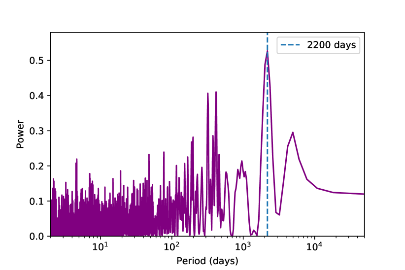
We also recovered a signal with a period of 18.3 days. There is significant periodicity in the S-value time series, a periodogram of which is shown in Figure 28. However, it is concentrated around a period of 6 yr, and there is no significant power near 18.3 days. Furthermore, we find no correlation between the RVs and S-values. Thus, we report this signal as a confirmed planet, with $M\sin{i}$ = $19.9\pm 3.1$ $M_{\oplus}$ and $a=0.1406\pm 0.0018$ AU.

Figure 27: RVSearch summary plot for HD 107148. See Figure 6 for plot description.

Figure 28: Lomb-Scargle periodogram of HIRES S-values for HD 107148. Significant power at and beyond 4,300 days.

A.8 HD 136925

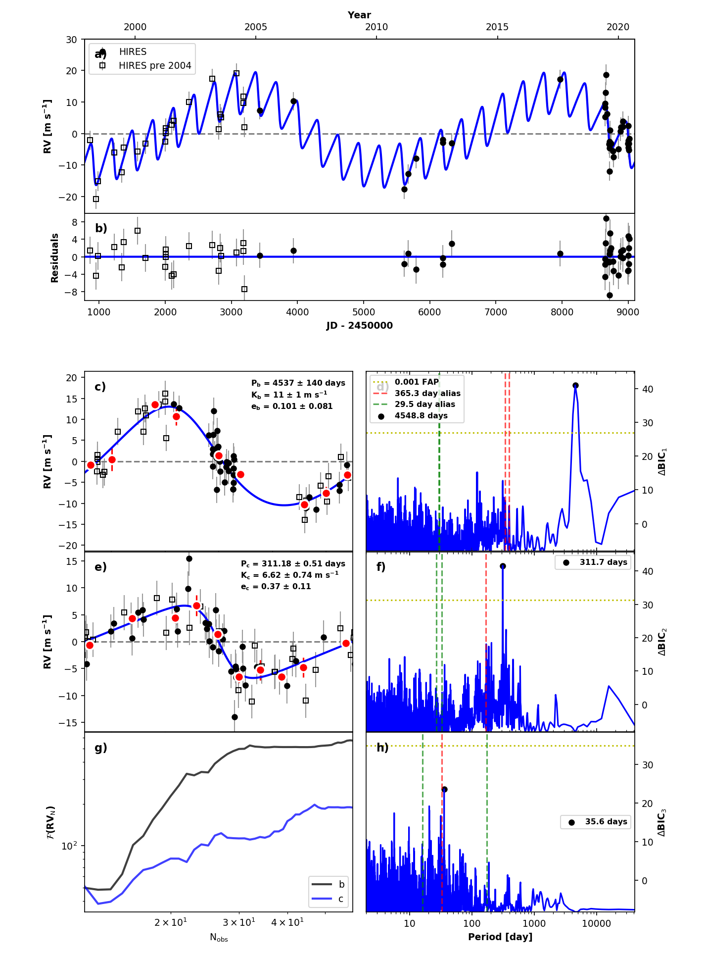
HD 136925 is a G0 dwarf, found at a distance of 47.9 pc. RVSearch detected two periodic signals in this dataset, as seen in Figure 29, at 311 days and 12.4 yr. This dataset is currently sparse, with two gaps of several years in the post-upgrade HIRES data, but there is clear long-period variation in the RVs. Keplerian modeling predicts $M\sin{i}$ = 0.84 $M_{\textrm{J}}$ for the giant planet.

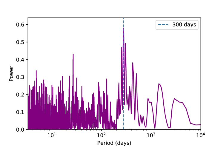
The S-value periodogram seen in Figure 30 shows no significant power beyond 1000 days, suggesting that the long-period HD 136925 b is a real planet. There is broad power around 300 days, overlapping with the period of the inner signal. It is unclear whether this periodicity is caused by real stellar variability or is a product of sparse data. Table 1 reports current estimates of all planet parameters. We need more data in order to clarify our model, and determine whether the inner signal is caused by a planet or a product of stellar activity and sparse data. Therefore, we designated HD 136925 b as a planet, and the inner signal as a probable false positive, to be clarified with continued HIRES observing.

Figure 29: RVSearch summary plot for HD 136925. See Figure 6 for plot description.

Figure 30: RVSearch summary plot for HD 136925. Periodogram of HIRES S-values for HD 136925. Significant periodicity around 300 days, near the period of the inner signal.

A.9 HD 141004

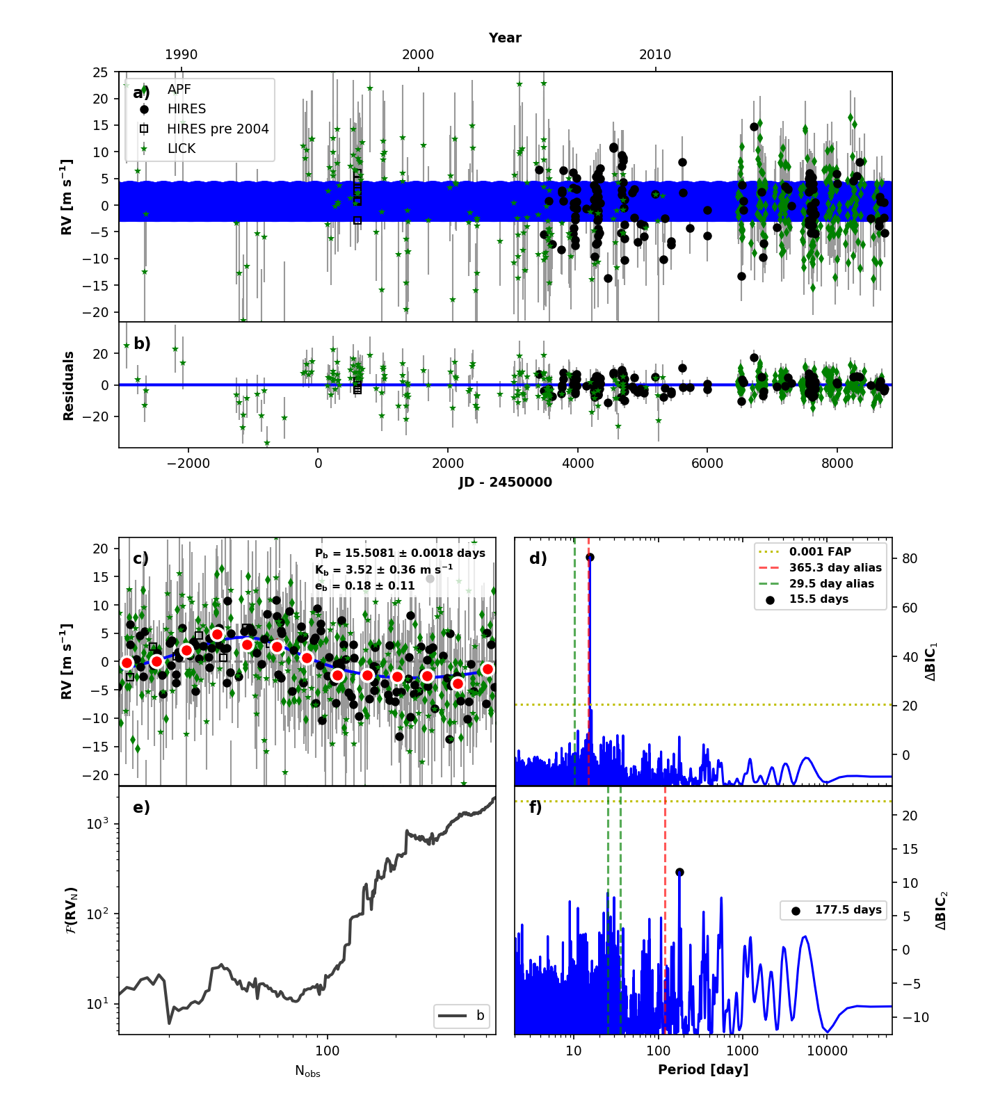
HD 141004 is a G0 dwarf found at a distance of 11.8 pc. Figure 31 shows the RVSearch results for this star. Roy et al. (2021, in preparation) discovered a sub-Neptune at an orbital period of 15.5 days, with $M\sin{i}$ = $13.9\ \pm 1.5$ $M_{\oplus}$, and will report on the analysis of this system in greater detail. Table 1 reports current estimates of all planet parameters.

Figure 31: RVSearch summary plot for HD 141004. See Figure 6 for plot description.

A.10 HD 145675

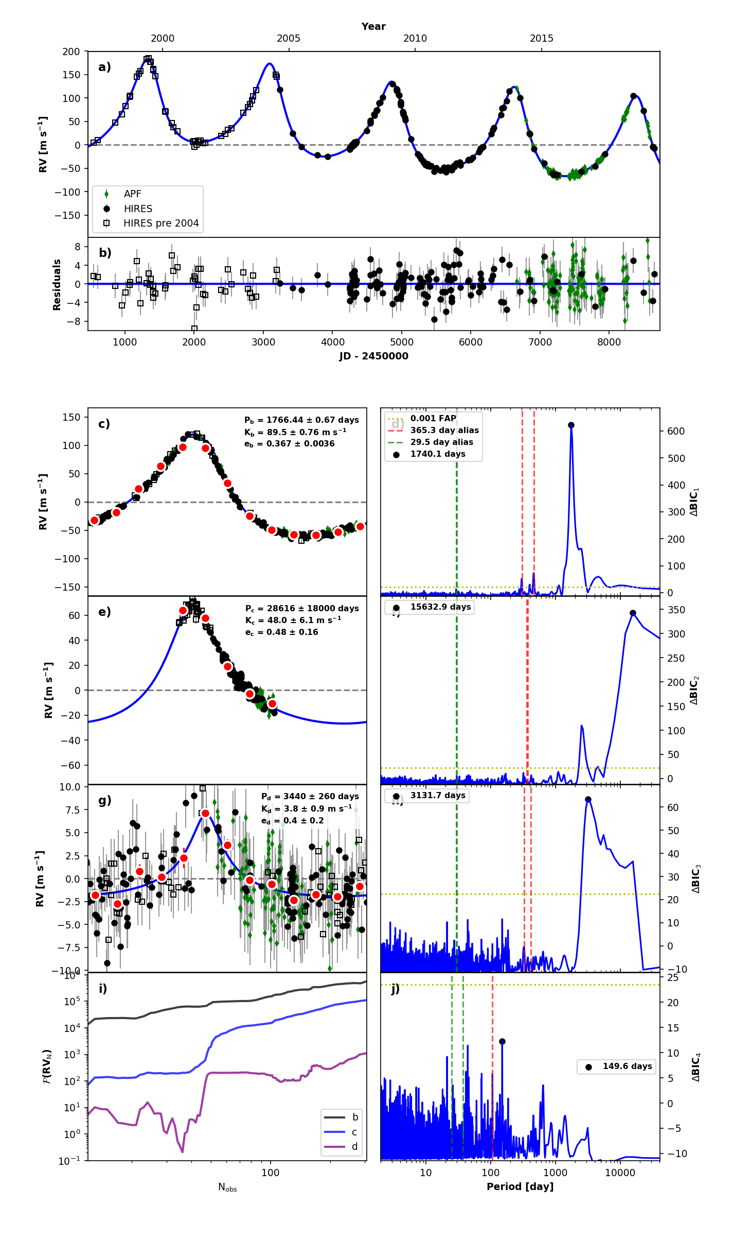
HD 145675 (14 Her) is a K0 dwarf found at a distance of 17.9 pc. Figure 32 shows the RVSearch results for this star. This system has one known cold gas giant, with $M\sin{i}$= 5.10 $M_{\textrm{J}}$ and an orbital period of 4.84 yr, which was first reported in Butler et al. (2003). Wittenmyer et al. (2007a) conducted further analysis with a longer observational baseline of twelve years, and noted a long-period trend. Wright et al. (2007) used additional RV curvature constraints to show that this trend must correspond to a companion with $P>12$ yr and $M\sin{i}$ $>$ 5 $M_{\textrm{J}}$. The observational baseline has since increased from 12 yr to 22, and regular observations with HIRES and APF allow us to place further constraints on this long-period companion. We find $M\sin{i}$ = 5.8$\mathrm{\begin{subarray}{c}+1.4\\ -1.0\end{subarray}}$ $M_{\textrm{J}}$, $P=68\mathrm{\begin{subarray}{c}+64\\ -25\end{subarray}}$ yr, semi-major axis $a=16.4\mathrm{\begin{subarray}{c}+9.3\\ -4.3\end{subarray}}$ AU, and eccentricity $e=0.45\mathrm{\begin{subarray}{c}+0.17\\ -0.15\end{subarray}}$. Table 1 reports all planet parameters.

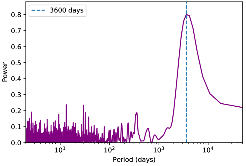
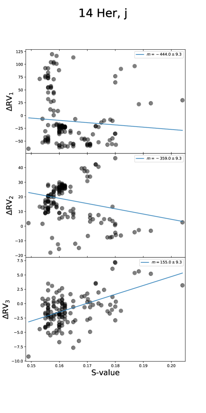
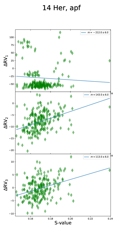
Figure 33 shows a Lomb–Scargle periodogram of the HIRES S-value time series. There is strong periodicity in the HIRES S-value time series, peaking around 10 yr, but no significant power near the supposed orbital period of the long-period candidate. These S-values strongly correlate with a third Keplerian signal picked up by our search, also with a period of 10 yr, as seen in the Figure 34, therefore we designate this signal as stellar activity.

There is a potential complication owed to a stellar binary candidate. Roberts et al. (2011) conducted a direct-imaging survey of known exoplanet hosts and reported a candidate stellar companion to 14 Her, with a differential magnitude of $10.9\pm 1.0$, an angular separation of 4.3”, and a minimum orbital separation of 78 AU. This is a single-epoch detection, and therefore could be only a visual binary. Additionally, Rodigas et al. (2011) conducted a deep direct imaging study of 14 Her, to constrain the mass and orbital parameters of 14 Her c, which, at the time, presented only as a parabolic trend in RV data. They used the Clio-2 photometer on the MMT, which has a 9” x 30” field of view; the authors only looked at imaging data within 2”, to filter out background stars. Although this deep imaging study did not mention any stellar companion, the candidate reported by Roberts et al. (2011) falls outside of their considered imaging data, which corresponds to a minimum separation of 112.8 AU. Wittrock et al. (2017) also found a null binary detection, using the Differential Speckle Survey Instrument (DSSI) at the Gemini-North Observatory. A 6 Jupiter mass object would not have been detected by the above surveys, as they were designed only to rule out stellar companions and therefore used shorter imaging exposures that would miss planetary-mass companions.

Additionally, we used Gaia DR2 to search for bound stellar companions within 10”, and found no such companions. We conclude that 14 Her does not have a bound stellar companion. Therefore, we designated 14 Her c as an eccentric, long-period planet. We will continue to monitor this star with Keck/HIRES and APF, to further constrain the orbit of this planet.

Figure 32: RVSearch summary plot for HD 145675. See Figure 6 for plot description.

Figure 33: Lomb-Scargle periodogram of HIRES S-values for HD 145675 showing significant power at 3,600 days.

Figure 34: Activity vetting plots for HD 145675. For all panels, the horizontal axis shows the S-value activity metric of each observation, while the vertical axis shows corresponding RV residuals for each individual Keplerian orbit. The left-hand panels show HIRES post-upgrade observations, while the right-hand panels show APF observations. Each row shows RVs with the model residuals of one Keplerian model, with the other Keplerian models subtracted from the data. The blue lines show linear correlations between these residuals and the corresponding S-values. In the HIRES and APF data, we measured $>3\sigma$ correlations for the third Keplerian signal. The APF and HIRES linear correlations are within $3\sigma$ of each other, implying that this signal is caused by stellar activity. We find correlations between the residuals and S-values for the second signal as well, but they are significantly different for HIRES and APF. Since the period of this signal is much greater than the APF baseline of this star, we discount this second correlation as caused by the limited baseline of the data with respect to the signal.

A.11 HD 156668

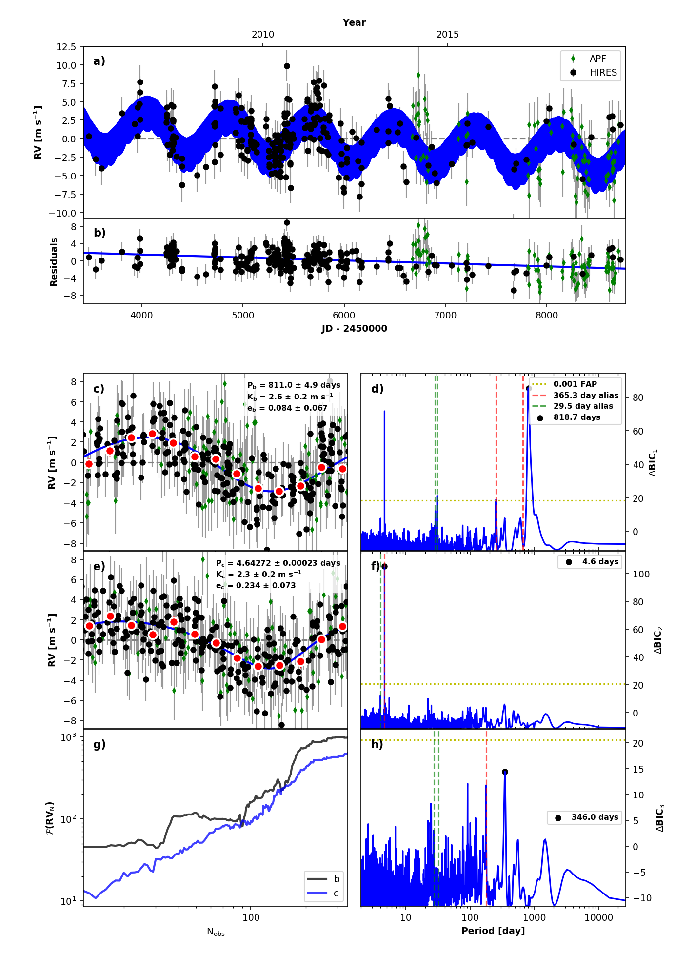
HD 156668 is a K3 dwarf found at a distance of 24.4 pc. Figure 35 shows the RVSearch results for this star. This system has one known short-period super-Earth, with $M\sin{i}$= 4.15 $M_{\oplus}$and an orbital period of 4.64 days. This planet was first reported by Howard et al. (2011), who also noted a long-period ($P\approx 2.3$ yr) signal with insufficient RV observations or additional data for confirmation as a planet. The observational baseline has since increased from five years to fourteen, allowing us to confirm this long-period signal as a planet with $M\sin{i}$ = 0.167 $M_{\textrm{J}}$ and an orbital period $P=2.22$ yr.

There is a strong periodicity in the HIRES S-value time series, peaking around 10 yr, but no significant power near the orbital period of the long-period candidate. If we do not model this activity, a one-year alias signal appears in the periodogram search (Fig. 35). The data do not sufficiently constrain a Keplerian fit with a 10 yr period, but we find that a linear trend models the activity well enough to remove the one-year alias from the search. We opt to include this linear trend, which we treat as a nuisance parameter.

Figure 35: RVSearch summary plot for HD 156668. See Figure 6 for plot description.

A.12 HD 164922

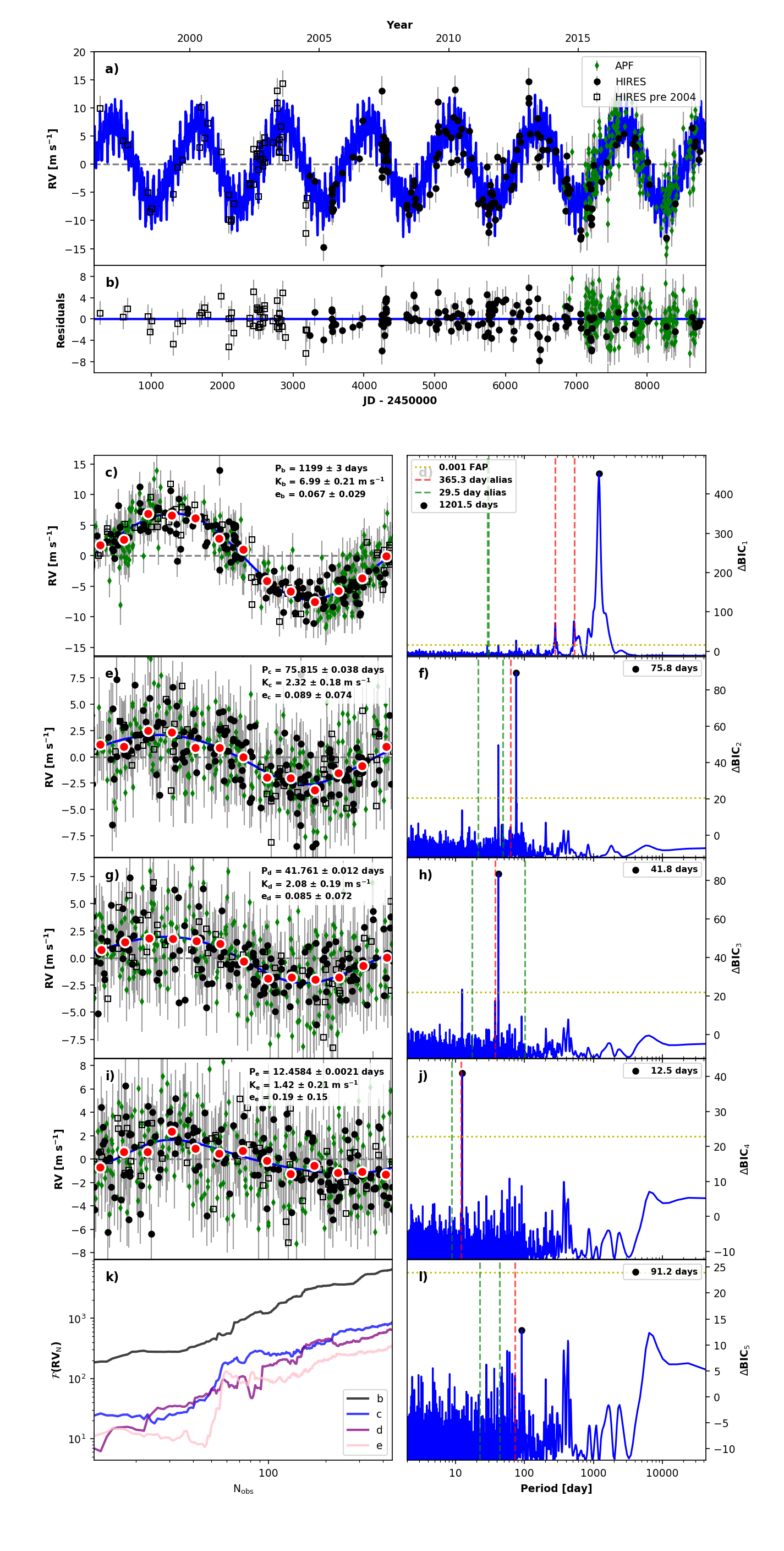
HD 164922 is a G9 V dwarf located at a distance of 22.1 pc. Figure 36 shows the RVSearch results for this star. It hosts two known planets: a 0.3 $M_{\textrm{J}}$ planet with an orbital period of 1207 days (Butler et al., 2006b), and a super-Earth with $M\sin{i}$ = 14.3 $M_{\oplus}$ and an orbital period of 75.8 days. This super-Earth was reported by Fulton et al. (2016), who also reported residual power around 41.7 days but did not find it significant enough to merit candidate status. With approximately two more years of HIRES and APF data, we identified the 41.7 day signal as a strong planet candidate and confirmed the 12.5 day planet reported in Benatti et al. (2020). Both planets are of sub-Neptune mass and have eccentricity posteriors that are consistent with circular orbits. The 41.7 day planet has $M\sin{i}$ = $10.7\pm 1.0$ $M_{\oplus}$  and a semi-major axis $a=0.2294\pm 0.0031$ AU. The 12.5 day planet has $M\sin{i}$ = $4.63\pm 0.70$ $M_{\oplus}$  and a semi-major axis $a=0.1024\pm 0.0014$ AU. Table 1 reports all planet parameters.

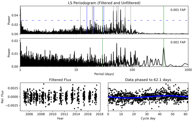
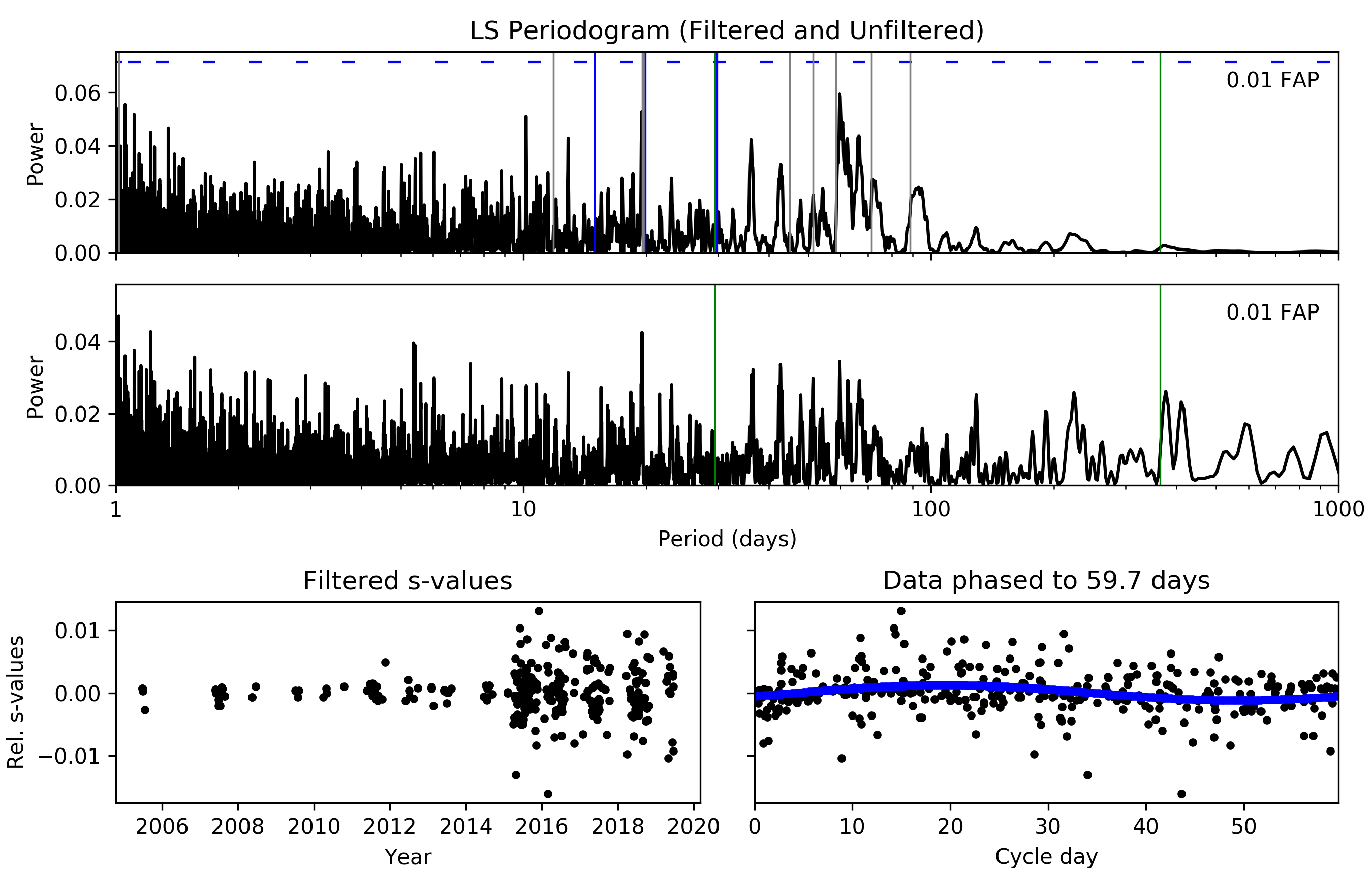
To validate these candidates, we searched for periodicity in both S-value activity metrics and APT photometry. We found no evidence for stellar rotation in S-values, but estimated a stellar rotation period of 62.1 days from our APT photometry. Figure 37 shows periodograms and a phase-folded curve from this APT analysis, and Figure 38 shows equivalent analysis for HIRES S-values. The 1 yr alias of 62.1 days is 75.8 days, but the 75.8 day planet detection is high-amplitude and clean, without an additional peak near 62 days in any of the RVSearch periodograms. Therefore, within the limits of our activity metrics and vetting process, we ruled out stellar rotation as a cause of the 41.7 day signal.

Benatti et al. (2020) used multiple HARPS-N spectral activity indicators to estimate a stellar rotation period of 41.6 days, and they note that this rotation period is to be expected from empirical activity-rotation relationships. Therefore, they determined that the strong 42 day signal present in their HARPS RVs is caused by rotation. However, we find no evidence of significant 42 day periodicity in our analysis of spectral activity indicators or APT photometry, as seen in Figures 37 and 38, and both datasets reflect significant periodicity near 60 days. Since our RV detection of this planet candidate is clean and does not conflict with our activity analysis, we chose to include this signal in our catalog as a planet candidate, to be confirmed or refuted by independent analysis.

Figure 36: RVSearch summary plot for HD 164922. See Figure 6 for plot description.

Figure 37: Visualization of APT photometry analysis for HD 164922. The top panel shows a Lomb-Scargle periodogram of the photometry, with a moving-average filter to reduce alias issues. The middle panel shows an unfiltered periodogram.

Figure 38: Visualization of HIRES S-value analysis for HD 164922. The top panel shows a Lomb-Scargle periodogram of the S-values, with a moving-average filter to reduce alias issues. The middle panel shows an unfiltered periodogram.

A.13 HD 168009

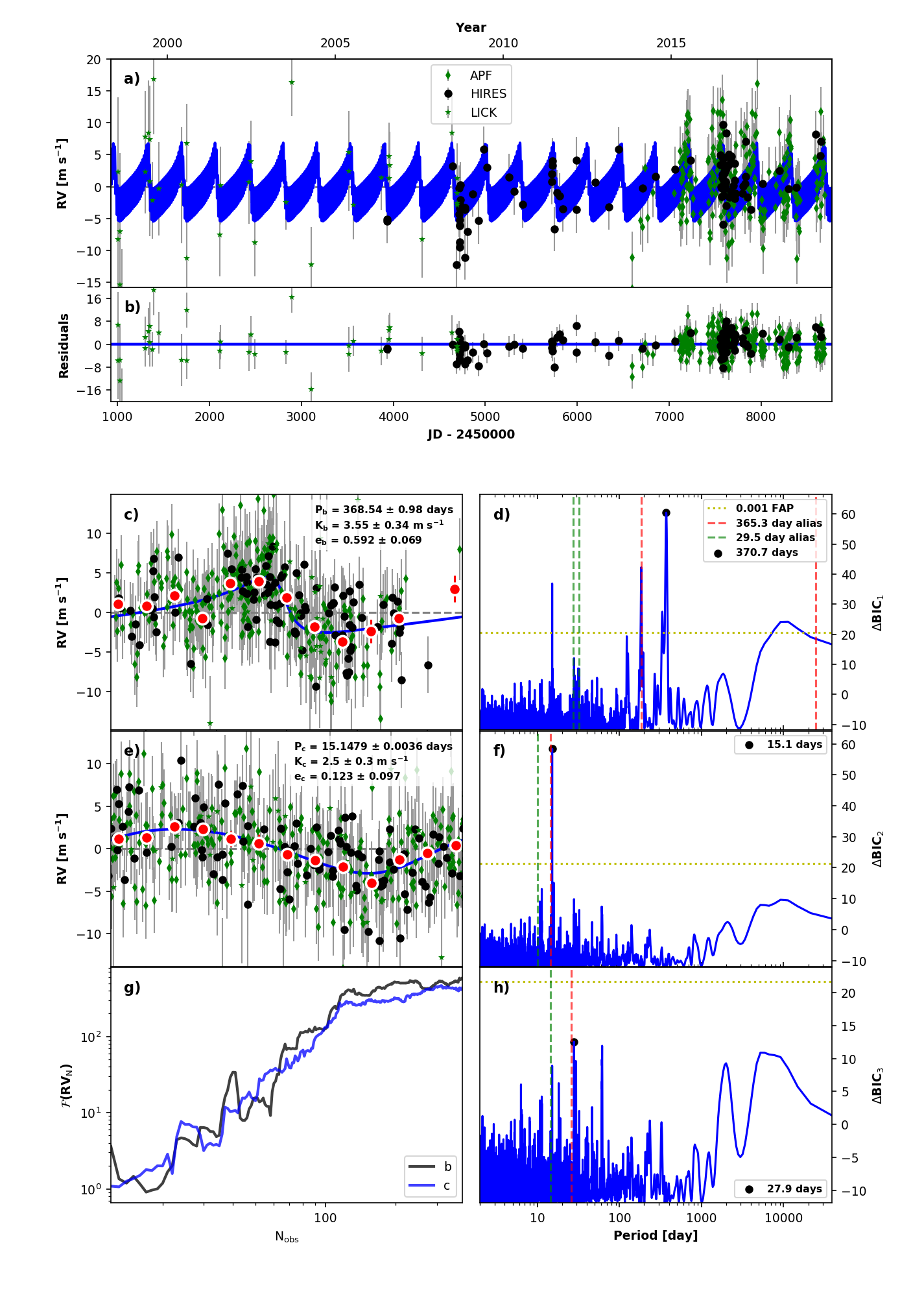
HD 168009 is a G1 dwarf found at a distance of 23.3 pc. Figure 39 shows the RVSearch results for this star. Roy et al. (2021, in preparation) discovered a super-Earth candidate at an orbital period of 15.5 days, with $M\sin{i}$ = $10.3\ \pm 1.1$ $M_{\oplus}$, and will report on the analysis of this candidate in greater detail. Table 1 reports current estimates of all planet parameters.

RVSearch also recovered a highly eccentric 1 yr signal, but this signal correlates with APF systematics. Therefore, we labeled it as a false positive. Roy et al. (2021, in preparation) will model these systematics in greater detail.

Figure 39: RVSearch summary plot for HD 168009. See Figure 6 for plot description.

A.14 HD 213472

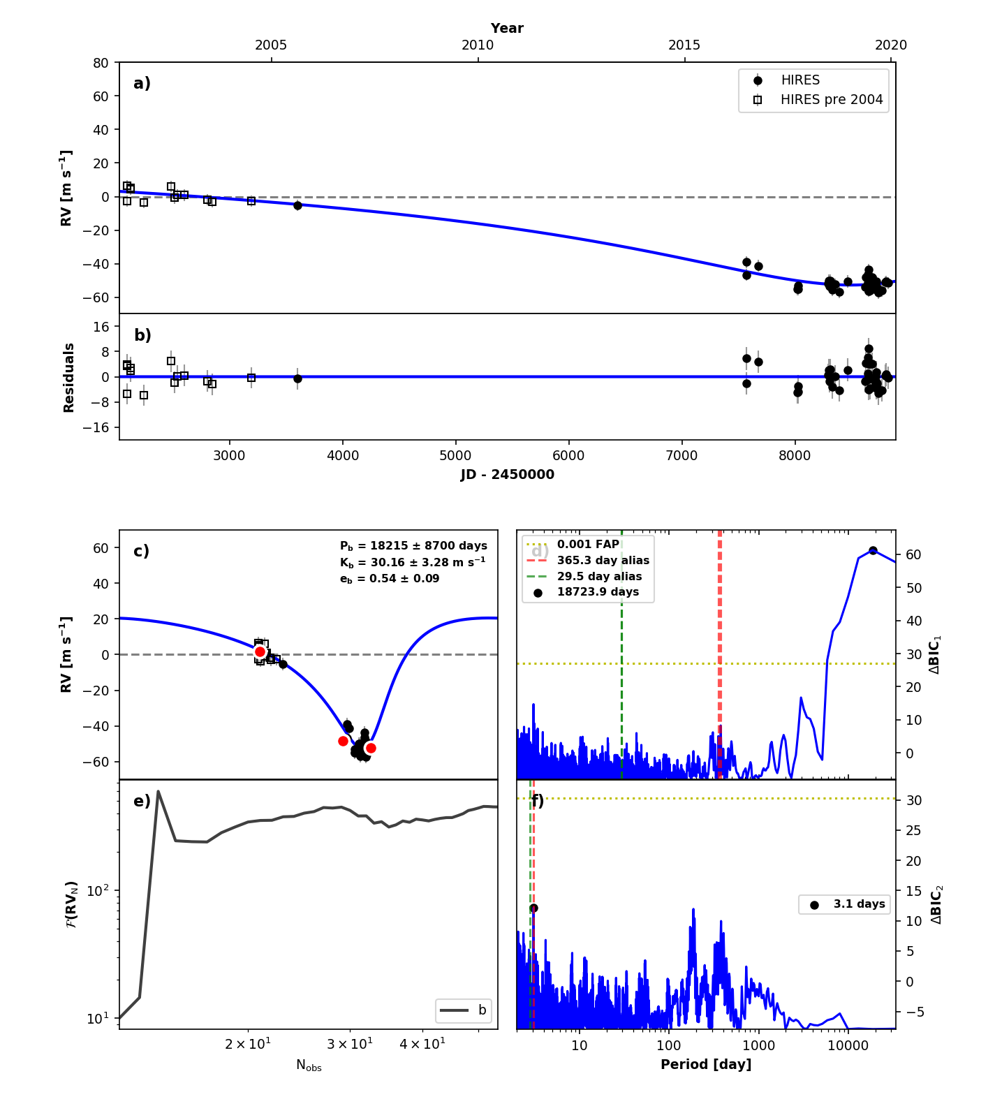
HD 213472 is a G5 dwarf located at a distance of 64.6 pc. Figure 40 shows the RVSearch results for this star. There is an approximately eleven-year gap in RV observations of this star. The first post-upgrade HIRES observation was measured in 2005, shortly after the last pre-upgrade observation, and the second post-upgrade observation was measured in 2016. The 40 m s^-1 difference between these two observations prompted the CPS team to begin observing HD 213472 regularly. Together with observations since 2016, and the thirteen pre-upgrade HIRES measurements, the data are consistent with a long-period, eccentric, planetary companion. Our periodogram search detects such a long-period signal. Due to the sparseness of the data, traditional MCMC methods fail to return a well-sampled model posterior. We used the rejection sampling algorithm TheJoker (Price-Whelan et al., 2017) to estimate the posterior, and found it to be unimodal. This model is consistent with a very long-period gas giant, with $M\sin{i}$ = $3.48\mathrm{\begin{subarray}{c}+1.10\\ -0.59\end{subarray}}$ $M_{\textrm{J}}$  orbital period $P=46\mathrm{\begin{subarray}{c}+33\\ -13\end{subarray}}$ yr, semi-major axis $a=13.0\mathrm{\begin{subarray}{c}+5.7\\ -2.6\end{subarray}}$ AU, and eccentricity of $e=0.53\mathrm{\begin{subarray}{c}+0.12\\ -0.09\end{subarray}}$. Table 1 reports all planet parameters. Figure 41 shows the orbital parameter posteriors generated by TheJoker.

To investigate the possibility of a stellar or substellar companion, we compared this Keplerian model to a simple linear trend by computing the $\Delta\mathrm{BIC}$ between the two max-likelihood models. The Keplerian model is significantly preferred with $\Delta\mathrm{BIC}$ = 23.7. Additionally, we used Gaia to search for bound companions within 10”, and found no such companions. Therefore, we inferred that HD 213472 b is either a planet or low-mass substellar companion, and not a wide-orbit stellar companion.

Figure 42 shows a sample of possible orbits for HD 213472 b, drawn from our rejection sampling posteriors and projected over the next decade. More HIRES observations will further constrain this object’s mass and orbital parameters.

Figure 40: RVSearch summary plot for HD 213472. See Figure 6 for plot description.

Figure 41: Rejection sampling posterior for HD 213472 b orbital parameters. $\Delta\gamma$ is the relative linear offset between different instrumental datasets, in this case pre-upgrade and post-upgrade HIRES.

Figure 42: Possible orbits for HD 213472 b. RV curves are drawn from the rejection sampling posterior generated with TheJoker. The color of each orbit drawn from the posterior scales with $M\sin{i}$ .

Appendix B Stellar Catalog

We record a subset of the stellar catalog and its associated stellar parameters in Table 2. We make this table of CLS stars available in its entirety in machine-readable format.

Table 2: Stellar Catalog

CPS Name	Lit. Name	$T_{\textrm{eff}}$ [K]	[Fe/H]	log $g$ [log(cm s-2)]	$R$ [R⊙]	$M$ [M⊙]
HD 10002	HD 10002	$5320.0\pm 100.0$	$0.251\pm 0.058$	$4.449\pm 0.03$	$0.949\pm 0.021$	$0.928\pm 0.04$
HD 10008	HIP 7576	$5390.0\pm 100.0$	$0.024\pm 0.059$	$4.553\pm 0.018$	$0.832\pm 0.014$	$0.897\pm 0.028$
HD 100180	HIP 56242 A	$5990.0\pm 100.0$	$0.009\pm 0.06$	$4.361\pm 0.032$	$1.125\pm 0.026$	$1.062\pm 0.049$
HD 100623	HIP 56452	$5110.0\pm 100.0$	$-0.321\pm 0.059$	$4.576\pm 0.022$	$0.734\pm 0.012$	$0.748\pm 0.028$
HD 101259	HD 101259	$4960.0\pm 100.0$	$-0.634\pm 0.061$	$3.178\pm 0.059$	$4.72\pm 0.11$	$1.23\pm 0.15$
HD 10145	HD 10145	$5610.0\pm 100.0$	$0.004\pm 0.058$	$4.333\pm 0.027$	$1.08\pm 0.025$	$0.921\pm 0.036$

Appendix C Known Planets

We record all planets recovered by RVSearch in Table 3, with $M\sin{i}$ and key orbital parameter medians and uncertainties. We record all fitting parameter values in machine-readable format.

Table 3: Planet Catalog

CPS Name	Lit. Name	$M\sin{i}$ [$M_{\textrm{J}}$]	$a$ [AU]	$e$	Ref.
HD 104067 b	HD 104067 b	$0.202^{+0.017}_{-0.017}$	$0.2673^{+0.0032}_{-0.0033}$	$0.247^{+0.080}_{-0.082}$	Vogt et al. (2000)
HD 10697 b	HD 10697 b	$6.39^{+0.13}_{-0.13}$	$2.156^{+0.02}_{-0.02}$	$0.0998^{+0.0082}_{-0.0082}$	Butler et al. (2006b)
HD 107148 b	HD 107148 b	$0.203^{+0.015}_{-0.015}$	$0.3668^{+0.0047}_{-0.0048}$	$0.174^{+0.071}_{-0.075}$	Butler et al. (2006b)
HD 107148 c	HD 107148 c	$0.0626^{+0.0097}_{-0.0098}$	$0.1406^{+0.0018}_{-0.0018}$	$0.34^{+0.13}_{-0.16}$	This work
HD 108874 b	HD 108874 b	$1.32^{+0.047}_{-0.047}$	$1.053^{+0.016}_{-0.016}$	$0.144^{+0.016}_{-0.016}$	Butler et al. (2003)
HD 108874 c	HD 108874 c	$1.14^{+0.052}_{-0.050}$	$2.83^{+0.044}_{-0.045}$	$0.265^{+0.030}_{-0.031}$	Vogt et al. (2005)
HD 114729 b	HD 114729 b	$0.892^{+0.053}_{-0.053}$	$2.094^{+0.022}_{-0.022}$	$0.098^{+0.048}_{-0.050}$	Butler et al. (2003)
HD 114783 b	HD 114783 b	$1.033^{+0.034}_{-0.033}$	$1.164^{+0.016}_{-0.016}$	$0.126^{+0.016}_{-0.016}$	Vogt et al. (2002)
HD 114783 c	HD 114783 c	$0.66^{+0.046}_{-0.047}$	$4.97^{+0.12}_{-0.11}$	$0.114^{+0.058}_{-0.058}$	Bryan et al. (2016)
HD 115617 b	61 Vir b	$0.0507^{+0.0035}_{-0.0036}$	$0.215^{+0.0028}_{-0.0029}$	$0.068^{+0.067}_{-0.047}$	Vogt et al. (2010)
HD 115617 c	61 Vir c	$0.0161^{+0.0017}_{-0.0016}$	$0.04956^{+0.00066}_{-0.00067}$	$0.099^{+0.091}_{-0.070}$	Vogt et al. (2010)
HD 117176 b	70 Vir b	$7.24^{+0.13}_{-0.13}$	$0.4766^{+0.0043}_{-0.0044}$	$0.3989^{+0.0011}_{-0.0012}$	Butler & Marcy (1996)
HD 117207 b	HD 117207 b	$1.87^{+0.076}_{-0.075}$	$3.744^{+0.059}_{-0.060}$	$0.142^{+0.027}_{-0.026}$	Marcy et al. (2005)
HD 11964a b	HD 11964a b	$0.631^{+0.027}_{-0.027}$	$3.185^{+0.032}_{-0.032}$	$0.101^{+0.044}_{-0.046}$	Butler et al. (2006b)
HD 11964a c	HD 11964a c	$0.0766^{+0.0063}_{-0.0061}$	$0.2315^{+0.0022}_{-0.0022}$	$0.106^{+0.088}_{-0.071}$	Wright et al. (2009)
HD 120066 b	HR 5183 b	$3.15^{+0.18}_{-0.17}$	$25.0^{+19.0}_{-8.3}$	$0.886^{+0.049}_{-0.056}$	Blunt et al. (2019)
HD 120136 b	tau Boo b	$4.3^{+0.075}_{-0.075}$	$0.04869^{+0.00039}_{-0.00040}$	$0.0074^{+0.0059}_{-0.0048}$	Butler et al. (1997)
HD 12661 b	HD 12661 b	$2.283^{+0.062}_{-0.063}$	$0.824^{+0.011}_{-0.011}$	$0.3597^{+0.0046}_{-0.0044}$	Fischer et al. (2001)
HD 12661 c	HD 12661 c	$1.855^{+0.054}_{-0.054}$	$2.86^{+0.038}_{-0.039}$	$0.025^{+0.012}_{-0.012}$	Fischer et al. (2003)
HD 126614 b	HD 126614 b	$0.356^{+0.032}_{-0.030}$	$2.291^{+0.026}_{-0.027}$	$0.577^{+0.069}_{-0.065}$	Howard et al. (2010a)
HD 128311 b	HD 128311 b	$3.25^{+0.12}_{-0.12}$	$1.742^{+0.020}_{-0.021}$	$0.196^{+0.047}_{-0.057}$	Butler et al. (2003)
HD 128311 c	HD 128311 c	$2.0^{+0.15}_{-0.15}$	$1.088^{+0.012}_{-0.013}$	$0.283^{+0.04}_{-0.04}$	Vogt et al. (2005)
HD 130322 b	HD 130322 b	$1.149^{+0.037}_{-0.036}$	$0.0929^{+0.0011}_{-0.0011}$	$0.015^{+0.016}_{-0.010}$	Udry et al. (2000)
HD 1326 b	HD 1326 b	$0.0171^{+0.0013}_{-0.0013}$	$0.07321^{+0.00047}_{-0.00048}$	$0.075^{+0.072}_{-0.052}$	Howard et al. (2014)
HD 134987 b	HD 134987 b	$1.623^{+0.049}_{-0.049}$	$0.817^{+0.012}_{-0.012}$	$0.2281^{+0.0078}_{-0.0077}$	Vogt et al. (2000)
HD 134987 c	HD 134987 c	$0.934^{+0.063}_{-0.060}$	$6.62^{+0.16}_{-0.15}$	$0.154^{+0.049}_{-0.050}$	Jones et al. (2010)
HD 136925 b	HD 136925 b	$0.84^{+0.078}_{-0.074}$	$5.13^{+0.12}_{-0.11}$	$0.103^{+0.094}_{-0.070}$	This work
HD 13931 b	HD 13931 b	$1.911^{+0.077}_{-0.076}$	$5.323^{+0.091}_{-0.091}$	$0.02^{+0.021}_{-0.014}$	Howard et al. (2010a)
HD 141004 b	HIP 77257 b	$0.0428^{+0.0047}_{-0.0045}$	$0.1238^{+0.002}_{-0.002}$	$0.16^{+0.11}_{-0.10}$	This work
HD 141399 b	HD 141399 b	$1.329^{+0.046}_{-0.047}$	$0.693^{+0.012}_{-0.012}$	$0.0465^{+0.0068}_{-0.0068}$	Vogt et al. (2014)
HD 141399 c	HD 141399 c	$1.263^{+0.047}_{-0.048}$	$2.114^{+0.036}_{-0.037}$	$0.044^{+0.013}_{-0.013}$	Vogt et al. (2014)
HD 141399 d	HD 141399 d	$0.452^{+0.017}_{-0.017}$	$0.4176^{+0.0070}_{-0.0073}$	$0.053^{+0.015}_{-0.015}$	Vogt et al. (2014)
HD 141399 e	HD 141399 e	$0.644^{+0.042}_{-0.040}$	$4.5^{+0.11}_{-0.11}$	$0.047^{+0.052}_{-0.033}$	Vogt et al. (2014)
HD 143761 b	rho CrB b	$1.057^{+0.024}_{-0.024}$	$0.2213^{+0.0025}_{-0.0025}$	$0.0355^{+0.0035}_{-0.0037}$	Noyes et al. (1997)
HD 143761 c	rho CrB c	$0.0885^{+0.0055}_{-0.0056}$	$0.4157^{+0.0046}_{-0.0047}$	$0.044^{+0.050}_{-0.031}$	Fulton et al. (2016)
HD 145675 b	14 Her b	$4.85^{+0.15}_{-0.14}$	$2.83^{+0.040}_{-0.041}$	$0.3674^{+0.0035}_{-0.0038}$	Wittenmyer et al. (2007b)
HD 145675 c	14 Her c	$5.8^{+1.4}_{-1.0}$	$16.4^{+9.3}_{-4.3}$	$0.45^{+0.17}_{-0.15}$	This work
HD 145934 b	HD 145934 b	$2.04^{+0.24}_{-0.23}$	$4.73^{+0.20}_{-0.21}$	$0.057^{+0.057}_{-0.039}$	Feng et al. (2015)
HD 1461 b	HD 1461 b	$0.0208^{+0.0019}_{-0.0018}$	$0.06361^{+0.00096}_{-0.00099}$	$0.062^{+0.060}_{-0.042}$	Rivera et al. (2010)
HD 1461 c	HD 1461 c	$0.0222^{+0.0028}_{-0.0028}$	$0.1121^{+0.0017}_{-0.0017}$	$0.112^{+0.10}_{-0.077}$	Mayor et al. (2011)
HD 147379A b	HD 147379A b	$0.096^{+0.012}_{-0.012}$	$0.3315^{+0.0024}_{-0.0024}$	$0.096^{+0.110}_{-0.068}$	Reiners et al. (2018)
HD 154345 b	HD 154345 b	$0.905^{+0.071}_{-0.089}$	$4.272^{+0.086}_{-0.080}$	$0.038^{+0.036}_{-0.027}$	Wright et al. (2007)
HD 156279 b	HD 156279 b	$9.5^{+0.31}_{-0.31}$	$0.5039^{+0.0082}_{-0.0084}$	$0.64779^{+0.00068}_{-0.00066}$	Díaz et al. (2012)
HD 156279 c	HD 156279 c	$9.44^{+0.31}_{-0.32}$	$5.46^{+0.091}_{-0.093}$	$0.2597^{+0.0050}_{-0.0049}$	Bryan et al. (2016)
HD 156668 b	HD 156668 b	$0.0991^{+0.0079}_{-0.0077}$	$1.57^{+0.017}_{-0.017}$	$0.089^{+0.084}_{-0.061}$	Howard et al. (2011)
HD 156668 c	HD 156668 c	$0.0158^{+0.0013}_{-0.0013}$	$0.05025^{+0.00050}_{-0.00051}$	$0.235^{+0.072}_{-0.072}$	This work
HD 16141 b	HD 16141 b	$0.25^{+0.017}_{-0.017}$	$0.3609^{+0.0072}_{-0.0075}$	$0.195^{+0.051}_{-0.051}$	Marcy et al. (2000)
HD 164922 b	HD 164922 b	$0.344^{+0.013}_{-0.013}$	$2.149^{+0.025}_{-0.025}$	$0.065^{+0.027}_{-0.029}$	Butler et al. (2006b)
HD 164922 c	HD 164922 c	$0.0451^{+0.0036}_{-0.0036}$	$0.3411^{+0.0039}_{-0.0040}$	$0.096^{+0.088}_{-0.066}$	Fulton et al. (2016)
HD 164922 d	HD 164922 d	$0.0331^{+0.0031}_{-0.0031}$	$0.2292^{+0.0026}_{-0.0027}$	$0.086^{+0.083}_{-0.060}$	This work
HD 164922 e	HD 164922 e	$0.0149^{+0.0021}_{-0.0021}$	$0.1023^{+0.0012}_{-0.0012}$	$0.18^{+0.17}_{-0.12}$	Benatti et al. (2020)
HD 167042 b	HD 167042 b	$1.59^{+0.13}_{-0.13}$	$1.304^{+0.040}_{-0.043}$	$0.092^{+0.061}_{-0.057}$	Johnson et al. (2008)
HD 168009 b	HIP 89474 b	$0.03^{+0.0038}_{-0.0037}$	$0.1192^{+0.0017}_{-0.0018}$	$0.121^{+0.110}_{-0.082}$	This work
HD 168443 b	HD 168443 b	$7.92^{+0.16}_{-0.16}$	$0.2977^{+0.0029}_{-0.0030}$	$0.5313^{+0.00062}_{-0.00061}$	Marcy et al. (1999)
HD 168443 c	HD 168443 c	$17.76^{+0.35}_{-0.35}$	$2.881^{+0.028}_{-0.029}$	$0.2112^{+0.0013}_{-0.0013}$	Marcy et al. (2001)
HD 168746 b	HD 168746 b	$0.2294^{+0.0078}_{-0.0075}$	$0.06504^{+0.00054}_{-0.00056}$	$0.098^{+0.026}_{-0.026}$	Pepe et al. (2002)
HD 169830 b	HD 169830 b	$2.957^{+0.069}_{-0.070}$	$0.8131^{+0.0082}_{-0.0085}$	$0.306^{+0.012}_{-0.013}$	Naef et al. (2001)
HD 169830 c	HD 169830 c	$3.51^{+0.12}_{-0.12}$	$3.283^{+0.035}_{-0.036}$	$0.257^{+0.019}_{-0.019}$	Mayor et al. (2004)
HD 170469 b	HD 170469 b	$0.555^{+0.075}_{-0.072}$	$2.212^{+0.040}_{-0.044}$	$0.15^{+0.16}_{-0.11}$	Fischer et al. (2007)
HD 177830 b	HD 177830 b	$1.347^{+0.097}_{-0.098}$	$1.179^{+0.040}_{-0.043}$	$0.028^{+0.017}_{-0.017}$	Vogt et al. (2000)
HD 177830 c	HD 177830 c	$0.104^{+0.016}_{-0.015}$	$0.496^{+0.017}_{-0.018}$	$0.54^{+0.12}_{-0.15}$	Meschiari et al. (2011)
HD 178911B b	HD 178911B b	$7.07^{+0.22}_{-0.23}$	$0.34^{+0.0053}_{-0.0055}$	$0.1132^{+0.0025}_{-0.0025}$	Zucker et al. (2002)
HD 179949 b	HD 179949 b	$0.966^{+0.031}_{-0.030}$	$0.04439^{+0.00045}_{-0.00046}$	$0.016^{+0.017}_{-0.011}$	Tinney et al. (2001)
HD 181234 b	HD 181234 b	$8.9^{+1.90}_{-0.76}$	$7.48^{+0.39}_{-0.23}$	$0.793^{+0.086}_{-0.082}$	Rickman et al. (2019)
HD 186427 b	16 Cyg B b	$1.752^{+0.054}_{-0.054}$	$1.676^{+0.025}_{-0.026}$	$0.6832^{+0.0031}_{-0.0031}$	Cochran et al. (1997)
HD 187123 b	HD 187123 b	$0.501^{+0.016}_{-0.016}$	$0.04185^{+0.00065}_{-0.00067}$	$0.004^{+0.0040}_{-0.0028}$	Butler et al. (1998)
HD 187123 c	HD 187123 c	$1.713^{+0.058}_{-0.058}$	$4.431^{+0.071}_{-0.072}$	$0.227^{+0.016}_{-0.017}$	Wright et al. (2009)
HD 188015 b	HD 188015 b	$1.455^{+0.060}_{-0.059}$	$1.187^{+0.018}_{-0.019}$	$0.17^{+0.025}_{-0.026}$	Marcy et al. (2005)
HD 189733 b	HD 189733 b	$1.162^{+0.036}_{-0.035}$	$0.03126^{+0.00036}_{-0.00037}$	$0.027^{+0.021}_{-0.018}$	Bouchy et al. (2005)
HD 190360 b	HD 190360 b	$1.492^{+0.043}_{-0.043}$	$3.955^{+0.052}_{-0.053}$	$0.3274^{+0.0081}_{-0.0087}$	Naef et al. (2003)
HD 190360 c	HD 190360 c	$0.0674^{+0.0027}_{-0.0026}$	$0.1294^{+0.0017}_{-0.0017}$	$0.165^{+0.027}_{-0.028}$	Vogt et al. (2005)
HD 192263 b	HD 192263 b	$0.658^{+0.03}_{-0.03}$	$0.154^{+0.0019}_{-0.0020}$	$0.04^{+0.037}_{-0.027}$	Santos et al. (2000)
HD 192310 b	HD 192310 b	$0.0451^{+0.0064}_{-0.0060}$	$0.3262^{+0.0035}_{-0.0037}$	$0.14^{+0.120}_{-0.093}$	Howard et al. (2011)
HD 195019 b	HD 195019 b	$3.655^{+0.091}_{-0.090}$	$0.1376^{+0.0017}_{-0.0017}$	$0.0198^{+0.0032}_{-0.0032}$	Fischer et al. (1999)
HD 209458 b	HD 209458 b	$0.665^{+0.022}_{-0.022}$	$0.04635^{+0.00068}_{-0.00070}$	$0.0105^{+0.0110}_{-0.0074}$	Henry et al. (2000)
HD 210277 b	HD 210277 b	$1.236^{+0.032}_{-0.033}$	$1.123^{+0.014}_{-0.014}$	$0.472^{+0.0055}_{-0.0056}$	Marcy et al. (1999)
HD 213472 b	HD 213472 b	$3.48^{+1.10}_{-0.59}$	$13.0^{+5.7}_{-2.6}$	$0.53^{+0.120}_{-0.085}$	This work
HD 216520 b	HIP 112527 b	$0.0326^{+0.0036}_{-0.0038}$	$0.1954^{+0.0025}_{-0.0025}$	$0.19^{+0.13}_{-0.12}$	Burt et al. 2020
HD 217014 b	51 Peg b	$0.464^{+0.014}_{-0.014}$	$0.05236^{+0.00076}_{-0.00079}$	$0.0042^{+0.0046}_{-0.0030}$	Mayor & Queloz (1995)
HD 217107 b	HD 217107 b	$1.385^{+0.039}_{-0.039}$	$0.0739^{+0.0010}_{-0.0011}$	$0.1279^{+0.0017}_{-0.0016}$	Fischer et al. (1999)
HD 217107 c	HD 217107 c	$4.31^{+0.13}_{-0.13}$	$5.944^{+0.083}_{-0.086}$	$0.3928^{+0.0069}_{-0.0067}$	Vogt et al. (2005)
HD 218566 b	HD 218566 b	$0.198^{+0.018}_{-0.018}$	$0.6875^{+0.0082}_{-0.0085}$	$0.268^{+0.10}_{-0.095}$	Meschiari et al. (2011)
HD 219134 b	HD 219134 b	$0.308^{+0.014}_{-0.014}$	$2.968^{+0.037}_{-0.037}$	$0.025^{+0.027}_{-0.018}$	Vogt et al. (2015)
HD 219134 c	HD 219134 c	$0.0516^{+0.0032}_{-0.0030}$	$0.2346^{+0.0026}_{-0.0027}$	$0.077^{+0.055}_{-0.050}$	Vogt et al. (2015)
HD 219134 d	HD 219134 d	$0.013^{+0.0010}_{-0.0011}$	$0.03838^{+0.00043}_{-0.00043}$	$0.063^{+0.070}_{-0.045}$	Vogt et al. (2015)
HD 219134 e	HD 219134 e	$0.0243^{+0.0023}_{-0.0022}$	$0.1453^{+0.0016}_{-0.0016}$	$0.072^{+0.078}_{-0.051}$	Vogt et al. (2015)
HD 219134 f	HD 219134 f	$0.0112^{+0.0014}_{-0.0014}$	$0.06466^{+0.00073}_{-0.00073}$	$0.16^{+0.12}_{-0.11}$	Vogt et al. (2015)
HD 22049 b	eps Eri b	$0.651^{+0.039}_{-0.039}$	$3.5^{+0.039}_{-0.040}$	$0.044^{+0.047}_{-0.031}$	Hatzes et al. (2000)
HD 222582 b	HD 222582 b	$7.88^{+0.24}_{-0.24}$	$1.335^{+0.02}_{-0.02}$	$0.7615^{+0.0035}_{-0.0034}$	Vogt et al. (2000)
HD 24040 b	HD 24040 b	$4.05^{+0.15}_{-0.15}$	$4.708^{+0.076}_{-0.077}$	$0.0117^{+0.0110}_{-0.0082}$	Boisse et al. (2012)
HD 24040 c	HD 24040 c	$0.201^{+0.027}_{-0.027}$	$1.3^{+0.021}_{-0.021}$	$0.11^{+0.120}_{-0.079}$	This work
HD 26161 b	HD 26161 b	$13.5^{+8.5}_{-3.7}$	$20.4^{+7.9}_{-4.9}$	$0.82^{+0.061}_{-0.050}$	This work
HD 28185 b	HD 28185 b	$6.04^{+0.2}_{-0.2}$	$1.045^{+0.016}_{-0.018}$	$0.0629^{+0.0042}_{-0.0049}$	Santos et al. (2001)
HD 285968 b	HD 285968 b	$0.0285^{+0.0043}_{-0.0043}$	$0.06649^{+0.00042}_{-0.00043}$	$0.16^{+0.14}_{-0.11}$	Forveille et al. (2009)
HD 31253 b	HD 31253 b	$0.446^{+0.063}_{-0.063}$	$1.296^{+0.024}_{-0.025}$	$0.44^{+0.12}_{-0.17}$	Meschiari et al. (2011)
HD 32963 b	HD 32963 b	$0.726^{+0.036}_{-0.035}$	$3.416^{+0.058}_{-0.059}$	$0.069^{+0.040}_{-0.039}$	Rowan et al. (2016)
HD 33636 b	HIP 24205 b	$8.92^{+0.29}_{-0.30}$	$3.238^{+0.051}_{-0.053}$	$0.491^{+0.0050}_{-0.0049}$	Vogt et al. (2002)
HD 34445 b	HD 34445 b	$0.658^{+0.04}_{-0.04}$	$2.106^{+0.038}_{-0.040}$	$0.103^{+0.059}_{-0.056}$	Howard et al. (2010a)
HD 3651 b	HD 3651 b	$0.2202^{+0.0077}_{-0.0077}$	$0.2954^{+0.0043}_{-0.0044}$	$0.614^{+0.015}_{-0.015}$	Fischer et al. (2003)
HD 3765 b	HIP 3206 b	$0.173^{+0.014}_{-0.013}$	$2.108^{+0.032}_{-0.033}$	$0.298^{+0.078}_{-0.071}$	This work
HD 38529 b	HD 38529 b	$13.21^{+0.1}_{-0.1}$	$3.736^{+0.01}_{-0.01}$	$0.3545^{+0.0048}_{-0.0047}$	Fischer et al. (2001)
HD 38529 c	HD 38529 c	$0.876^{+0.014}_{-0.014}$	$0.1329^{+0.00035}_{-0.00035}$	$0.26^{+0.014}_{-0.015}$	Fischer et al. (2003)
HD 40979 b	HD 40979 b	$3.8^{+0.16}_{-0.16}$	$0.8669^{+0.0074}_{-0.0076}$	$0.251^{+0.028}_{-0.028}$	Fischer et al. (2003)
HD 4203 b	HD 4203 b	$1.821^{+0.078}_{-0.077}$	$1.177^{+0.021}_{-0.022}$	$0.513^{+0.013}_{-0.014}$	Vogt et al. (2002)
HD 4203 c	HD 4203 c	$2.68^{+0.99}_{-0.24}$	$7.8^{+5.40}_{-0.78}$	$0.19^{+0.290}_{-0.089}$	Kane et al. (2014)
HD 4208 b	HD 4208 b	$0.771^{+0.036}_{-0.035}$	$1.634^{+0.022}_{-0.022}$	$0.059^{+0.044}_{-0.038}$	Vogt et al. (2002)
HD 42618 b	HD 42618 b	$0.0478^{+0.0057}_{-0.0056}$	$0.5337^{+0.0089}_{-0.0090}$	$0.27^{+0.13}_{-0.12}$	Fulton et al. (2016)
HD 45184 b	HD 45184 b	$0.0374^{+0.0040}_{-0.0038}$	$0.0641^{+0.0010}_{-0.0011}$	$0.18^{+0.1}_{-0.1}$	Mayor et al. (2011)
HD 45184 c	HD 45184 c	$0.0345^{+0.0057}_{-0.0059}$	$0.1095^{+0.0018}_{-0.0019}$	$0.48^{+0.18}_{-0.24}$	Udry et al. (2019)
HD 45350 b	HD 45350 b	$1.821^{+0.075}_{-0.070}$	$1.958^{+0.029}_{-0.030}$	$0.794^{+0.012}_{-0.012}$	Marcy et al. (2005)
HD 46375 b	HD 46375 b	$0.2267^{+0.0087}_{-0.0087}$	$0.03998^{+0.00059}_{-0.00060}$	$0.063^{+0.024}_{-0.024}$	Marcy et al. (2000)
HD 49674 b	HD 49674 b	$0.1149^{+0.0083}_{-0.0084}$	$0.058^{+0.00082}_{-0.00084}$	$0.06^{+0.060}_{-0.042}$	Butler et al. (2003)
HD 50499 b	HD 50499 b	$1.346^{+0.084}_{-0.087}$	$3.847^{+0.038}_{-0.040}$	$0.348^{+0.046}_{-0.045}$	Vogt et al. (2005)
HD 50499 c	HD 50499 c	$3.18^{+0.63}_{-0.46}$	$10.1^{+2.00}_{-0.84}$	$0.241^{+0.089}_{-0.075}$	Rickman et al. (2019)
HD 50554 b	HD 50554 b	$4.35^{+0.19}_{-0.18}$	$2.265^{+0.035}_{-0.036}$	$0.459^{+0.019}_{-0.018}$	Fischer et al. (2002)
HD 52265 b	HD 52265 b	$1.108^{+0.031}_{-0.031}$	$0.506^{+0.0056}_{-0.0056}$	$0.213^{+0.013}_{-0.014}$	Butler et al. (2000)
HD 66428 b	HD 66428 b	$3.19^{+0.11}_{-0.11}$	$3.455^{+0.049}_{-0.050}$	$0.418^{+0.015}_{-0.014}$	Butler et al. (2006b)
HD 66428 c	HD 66428 c	$27^{+22}_{-17}$	$23.0^{+19.0}_{-7.6}$	$0.32^{+0.23}_{-0.16}$	This work
HD 68988 b	HD 68988 b	$1.915^{+0.053}_{-0.054}$	$0.07021^{+0.00096}_{-0.0010}$	$0.1581^{+0.0027}_{-0.0031}$	Vogt et al. (2002)
HD 68988 c	HD 68988 c	$15.0^{+2.8}_{-1.5}$	$13.2^{+5.3}_{-2.0}$	$0.45^{+0.130}_{-0.081}$	This work
HD 69830 b	HD 69830 b	$0.0323^{+0.0021}_{-0.0020}$	$0.0794^{+0.0012}_{-0.0013}$	$0.112^{+0.054}_{-0.060}$	Lovis et al. (2006)
HD 69830 c	HD 69830 c	$0.031^{+0.003}_{-0.003}$	$0.1882^{+0.0029}_{-0.0030}$	$0.114^{+0.096}_{-0.079}$	Lovis et al. (2006)
HD 69830 d	HD 69830 d	$0.0444^{+0.0054}_{-0.0056}$	$0.645^{+0.01}_{-0.01}$	$0.104^{+0.10}_{-0.073}$	Lovis et al. (2006)
HD 72659 b	HD 72659 b	$2.85^{+0.12}_{-0.12}$	$4.652^{+0.067}_{-0.068}$	$0.269^{+0.018}_{-0.026}$	Butler et al. (2003)
HD 74156 b	HD 74156 b	$7.65^{+0.27}_{-0.26}$	$3.726^{+0.064}_{-0.065}$	$0.3691^{+0.0055}_{-0.0055}$	Naef et al. (2004)
HD 74156 c	HD 74156 c	$1.745^{+0.061}_{-0.061}$	$0.2844^{+0.0049}_{-0.0049}$	$0.6536^{+0.0036}_{-0.0038}$	Naef et al. (2004)
HD 75732 b	55 Cnc b	$0.841^{+0.026}_{-0.026}$	$0.1162^{+0.0018}_{-0.0018}$	$0.0048^{+0.0036}_{-0.0031}$	Butler et al. (1997)
HD 75732 c	55 Cnc c	$0.171^{+0.0066}_{-0.0067}$	$0.2432^{+0.0037}_{-0.0039}$	$0.048^{+0.031}_{-0.029}$	Marcy et al. (2002)
HD 75732 d	55 Cnc d	$2.86^{+0.25}_{-0.25}$	$5.54^{+0.1}_{-0.1}$	$0.139^{+0.015}_{-0.016}$	Marcy et al. (2002)
HD 75732 e	55 Cnc e	$0.1475^{+0.0093}_{-0.0094}$	$0.792^{+0.012}_{-0.013}$	$0.142^{+0.060}_{-0.066}$	McArthur et al. (2004)
HD 75732 f	55 Cnc f	$0.0295^{+0.0014}_{-0.0013}$	$0.01583^{+0.00024}_{-0.00025}$	$0.036^{+0.034}_{-0.025}$	Fischer et al. (2008)
HD 7924 b	HD 7924 b	$0.0259^{+0.0014}_{-0.0014}$	$0.05596^{+0.00075}_{-0.00079}$	$0.049^{+0.044}_{-0.035}$	Fulton et al. (2015)
HD 7924 c	HD 7924 c	$0.0278^{+0.0019}_{-0.0019}$	$0.1121^{+0.0015}_{-0.0016}$	$0.1^{+0.069}_{-0.062}$	Fulton et al. (2015)
HD 7924 d	HD 7924 d	$0.126^{+0.013}_{-0.012}$	$3.51^{+0.10}_{-0.096}$	$0.278^{+0.081}_{-0.082}$	Fulton et al. (2015)
HD 80606 b	HD 80606 b	$4.16^{+0.13}_{-0.13}$	$0.4602^{+0.0069}_{-0.0070}$	$0.93043^{+0.00068}_{-0.00069}$	Naef et al. (2001)
HD 82943 b	HD 82943 b	$1.652^{+0.085}_{-0.076}$	$0.747^{+0.011}_{-0.011}$	$0.421^{+0.014}_{-0.015}$	Mayor et al. (2004)
HD 82943 c	HD 82943 c	$1.539^{+0.052}_{-0.052}$	$1.189^{+0.017}_{-0.017}$	$0.142^{+0.042}_{-0.046}$	Mayor et al. (2004)
HD 8574 b	HD 8574 b	$1.765^{+0.075}_{-0.073}$	$0.75^{+0.012}_{-0.012}$	$0.306^{+0.022}_{-0.022}$	Perrier et al. (2003)
HD 87883 b	HD 87883 b	$2.292^{+0.069}_{-0.069}$	$4.073^{+0.056}_{-0.057}$	$0.7121^{+0.0083}_{-0.0079}$	Fischer et al. (2009)
HD 90156 b	HD 90156 b	$0.037^{+0.0062}_{-0.0060}$	$0.2508^{+0.0037}_{-0.0037}$	$0.16^{+0.18}_{-0.11}$	Mordasini et al. (2011)
HD 92788 b	HD 92788 b	$3.52^{+0.1}_{-0.1}$	$0.949^{+0.013}_{-0.013}$	$0.3552^{+0.0070}_{-0.0072}$	Fischer et al. (2001)
HD 92788 c	HD 92788 c	$2.81^{+0.18}_{-0.17}$	$8.26^{+0.37}_{-0.28}$	$0.355^{+0.057}_{-0.052}$	Rickman et al. (2019)
HD 95128 b	47 UMa b	$2.438^{+0.086}_{-0.085}$	$2.059^{+0.031}_{-0.033}$	$0.016^{+0.0076}_{-0.0080}$	Butler & Marcy (1996)
HD 95128 c	47 UMa c	$0.497^{+0.032}_{-0.030}$	$3.403^{+0.055}_{-0.056}$	$0.179^{+0.090}_{-0.092}$	Fischer et al. (2002)
HD 95128 d	47 UMa d	$1.51^{+0.22}_{-0.18}$	$13.8^{+4.8}_{-2.1}$	$0.38^{+0.16}_{-0.15}$	Gregory & Fischer (2010)
HD 95735 b	GJ 411 b	$0.0568^{+0.0091}_{-0.0083}$	$3.1^{+0.13}_{-0.11}$	$0.14^{+0.160}_{-0.095}$	Díaz et al. (2019)
HD 95735 c	GJ 411 c	$0.00882^{+0.00092}_{-0.00098}$	$0.07892^{+0.00055}_{-0.00054}$	$0.095^{+0.099}_{-0.066}$	This work
HD 97101 b	HD 97101 b	$0.184^{+0.010}_{-0.011}$	$1.424^{+0.011}_{-0.011}$	$0.185^{+0.069}_{-0.073}$	Dedrick et al. submitted
HD 97101 c	HD 97101 c	$0.0322^{+0.0043}_{-0.0038}$	$0.2403^{+0.0017}_{-0.0017}$	$0.28^{+0.13}_{-0.13}$	Dedrick et al. submitted
HD 97658 b	HD 97658 b	$0.0247^{+0.0018}_{-0.0017}$	$0.0805^{+0.0010}_{-0.0011}$	$0.063^{+0.061}_{-0.044}$	Howard et al. (2011)
HD 9826 b	ups And b	$0.675^{+0.016}_{-0.016}$	$0.05914^{+0.00062}_{-0.00063}$	$0.0069^{+0.0072}_{-0.0046}$	Butler et al. (1997)
HD 9826 c	ups And c	$1.965^{+0.049}_{-0.050}$	$0.8265^{+0.0087}_{-0.0088}$	$0.266^{+0.012}_{-0.012}$	Butler et al. (1999)
HD 9826 d	ups And d	$4.1^{+0.1}_{-0.1}$	$2.518^{+0.026}_{-0.027}$	$0.294^{+0.011}_{-0.012}$	Butler et al. (1999)
HD 99109 b	HD 99109 b	$0.474^{+0.035}_{-0.035}$	$1.122^{+0.017}_{-0.017}$	$0.06^{+0.064}_{-0.042}$	Butler et al. (2006b)
HD 99492 b	HD 99492 b	$0.0841^{+0.0061}_{-0.0062}$	$0.1231^{+0.0014}_{-0.0015}$	$0.085^{+0.070}_{-0.057}$	Marcy et al. (2005)
GL 317 b	GL 317 b	$1.852^{+0.037}_{-0.037}$	$1.1799^{+0.0076}_{-0.0076}$	$0.098^{+0.016}_{-0.016}$	Johnson et al. (2007a)
GL 317 c	GL 317 c	$1.673^{+0.078}_{-0.075}$	$5.78^{+0.74}_{-0.38}$	$0.248^{+0.110}_{-0.074}$	Anglada-Escudé et al. (2012)
GL 687 b	GL 687 b	$0.0553^{+0.0047}_{-0.0047}$	$0.1658^{+0.0012}_{-0.0012}$	$0.153^{+0.077}_{-0.080}$	Burt et al. (2014)
HIP 109388 b	GJ 849 b	$0.891^{+0.035}_{-0.036}$	$2.41^{+0.017}_{-0.017}$	$0.05^{+0.029}_{-0.030}$	Butler et al. (2006a)
HIP 109388 c	GJ 849 c	$1.079^{+0.053}_{-0.053}$	$4.974^{+0.082}_{-0.074}$	$0.099^{+0.041}_{-0.040}$	Feng et al. (2015)
HIP 22627 b	GJ 179 b	$0.752^{+0.041}_{-0.041}$	$2.522^{+0.034}_{-0.033}$	$0.169^{+0.048}_{-0.050}$	Howard et al. (2010a)
HIP 57050 b	GJ 1148 b	$0.26^{+0.030}_{-0.029}$	$0.9302^{+0.0088}_{-0.0086}$	$0.27^{+0.14}_{-0.17}$	Haghighipour et al. (2010)
HIP 57050 c	GJ 1148 c	$0.339^{+0.014}_{-0.014}$	$0.1686^{+0.0014}_{-0.0014}$	$0.366^{+0.027}_{-0.028}$	Trifonov et al. (2018)
HIP 74995 b	GJ 581 b	$0.051^{+0.0020}_{-0.0019}$	$0.04099^{+0.00043}_{-0.00044}$	$0.02^{+0.022}_{-0.014}$	Bonfils et al. (2005)
HIP 74995 c	GJ 581 c	$0.0159^{+0.0022}_{-0.0022}$	$0.07358^{+0.00077}_{-0.00078}$	$0.12^{+0.120}_{-0.084}$	Mayor et al. (2009)
HIP 83043 b	GJ 649 b	$0.275^{+0.022}_{-0.021}$	$1.1325^{+0.0087}_{-0.0087}$	$0.17^{+0.1}_{-0.1}$	Johnson et al. (2010a)
HIP 57087 b	GJ 436 b	$0.0668^{+0.0022}_{-0.0022}$	$0.02849^{+0.0002}_{-0.0002}$	$0.145^{+0.027}_{-0.027}$	Butler et al. (2004)
BD-103166 b	BD-103166 b	$0.449^{+0.017}_{-0.017}$	$0.04501^{+0.00064}_{-0.00066}$	$0.022^{+0.024}_{-0.015}$	Butler et al. (2000)
HD 175541 b	HD 175541 b	$0.577^{+0.049}_{-0.047}$	$0.99^{+0.030}_{-0.032}$	$0.057^{+0.053}_{-0.039}$	Johnson et al. (2007b)
HD 37124 b	HD 37124 b	$0.65^{+0.016}_{-0.016}$	$0.5253^{+0.0032}_{-0.0032}$	$0.05^{+0.019}_{-0.022}$	Butler et al. (2003)
HD 37124 c	HD 37124 c	$0.647^{+0.08}_{-0.09}$	$1.687^{+0.011}_{-0.011}$	$0.126^{+0.047}_{-0.045}$	Butler et al. (2003)
HD 37124 d	HD 37124 d	$0.659^{+0.034}_{-0.036}$	$2.67^{+0.022}_{-0.021}$	$0.16^{+0.12}_{-0.11}$	Vogt et al. (2005)
GL 876 b	GL 876 b	$2.108^{+0.036}_{-0.036}$	$0.2177^{+0.0018}_{-0.0018}$	$0.0019^{+0.0022}_{-0.0013}$	Marcy et al. (1998)
GL 876 c	GL 876 c	$0.698^{+0.013}_{-0.013}$	$0.1363^{+0.0011}_{-0.0011}$	$0.0055^{+0.0064}_{-0.0040}$	Marcy et al. (2001)
GL 876 d	GL 876 d	$0.0184^{+0.0016}_{-0.0015}$	$0.02183^{+0.00018}_{-0.00019}$	$0.273^{+0.093}_{-0.098}$	Rivera05
HD 83443 b	HD 83443 b	$0.409^{+0.019}_{-0.019}$	$0.04067^{+0.00060}_{-0.00062}$	$0.074^{+0.031}_{-0.032}$	Butler et al. (2002)
HD 183263 b	HD 183263 b	$3.705^{+0.098}_{-0.10}$	$1.508^{+0.02}_{-0.02}$	$0.3786^{+0.004}_{-0.004}$	Marcy et al. (2005)
HD 183263 c	HD 183263 c	$7.97^{+0.22}_{-0.22}$	$6.038^{+0.082}_{-0.085}$	$0.0595^{+0.0064}_{-0.0063}$	Wright et al. (2009)

Appendix D Resolved Binaries and Substellar Companions

We record all stellar binaries and substellar companions recovered by RVSearch in Table 4.

Table 4: Binary and Substellar Catalog

CPS Name	Lit. Name	$M\sin{i}$ [$M_{\textrm{J}}$]	$a$ [AU]	$e$
HD 104304	HIP 58576	$110.0^{+5.3}_{-6.1}$	$18.1^{+1.4}_{-1.6}$	$0.37^{+0.031}_{-0.035}$
HD 10790	HD 10790	$285^{+29}_{-20}$	$1.544^{+0.02}_{-0.02}$	$0.847^{+0.015}_{-0.011}$
HD 111031	HD 111031	$66^{+47}_{-33}$	$32^{+15}_{-10}$	$0.49^{+0.14}_{-0.17}$
HD 112914	HIP 63406	$223.1^{+4.6}_{-4.7}$	$1.389^{+0.016}_{-0.016}$	$0.32416^{+0.00036}_{-0.00037}$
HD 120136	tau Boo	$350^{+230}_{-160}$	$46^{+46}_{-18}$	$0.84^{+0.093}_{-0.140}$
HD 126614	HD 126614	$27.6^{+6.4}_{-5.1}$	$16.5^{+1.7}_{-1.5}$	$0.043^{+0.047}_{-0.031}$
HD 142229	HD 142229	$850^{+710}_{-470}$	$28^{+16}_{-11}$	$0.66^{+0.11}_{-0.13}$
HD 142267	HIP 77801	$141.2^{+2.6}_{-2.7}$	$0.4924^{+0.0048}_{-0.0050}$	$0.54768^{+0.00018}_{-0.00018}$
HD 144287	HIP 78709	$343^{+39}_{-29}$	$5.043^{+0.052}_{-0.053}$	$0.666^{+0.026}_{-0.022}$
HD 157338	HD 157338	$154^{+54}_{-47}$	$24.1^{+13.0}_{-6.1}$	$0.689^{+0.088}_{-0.062}$
HD 16160	HIP 12114	$67.3^{+1.5}_{-1.5}$	$16.37^{+0.28}_{-0.28}$	$0.6427^{+0.0038}_{-0.0039}$
HD 161797	HIP 86974	$238^{+60}_{-44}$	$22.2^{+4.4}_{-3.2}$	$0.427^{+0.069}_{-0.058}$
HD 167215	HD 167215	$201.1^{+4.2}_{-4.2}$	$7.205^{+0.077}_{-0.076}$	$0.8522^{+0.00059}_{-0.00066}$
HD 167215	HD 167215	$24.0^{+19.0}_{-4.3}$	$7.99^{+1.00}_{-0.51}$	$0.3^{+0.27}_{-0.20}$
HD 17382	HIP 13081	$197.9^{+4.5}_{-4.5}$	$5.967^{+0.072}_{-0.073}$	$0.6563^{+0.0058}_{-0.0061}$
HD 18445	HIP 13769 C	$33.8^{+7.0}_{-4.3}$	$1.209^{+0.016}_{-0.017}$	$0.67^{+0.120}_{-0.098}$
HD 185414	HIP 96395	$109.4^{+3.6}_{-3.7}$	$6.02^{+0.10}_{-0.11}$	$0.69345^{+0.00058}_{-0.00059}$
HD 190406	HIP 98819	$67.4^{+2.0}_{-2.0}$	$15.54^{+0.32}_{-0.31}$	$0.4618^{+0.0054}_{-0.0053}$
HD 211681	HD 211681	$76.4^{+3.3}_{-3.2}$	$7.79^{+0.21}_{-0.19}$	$0.4413^{+0.0076}_{-0.0064}$
HD 215578	HD 215578	$1405^{+50}_{-46}$	$25.8^{+1.3}_{-1.1}$	$0.477^{+0.018}_{-0.016}$
HD 239960	HIP 110893 A	$54^{+10}_{-13}$	$15.1^{+7.1}_{-5.0}$	$0.61^{+0.11}_{-0.14}$
HD 28185	HD 28185	$40^{+43}_{-28}$	$15.9^{+7.3}_{-5.1}$	$0.26^{+0.120}_{-0.093}$
HD 29461	HD 29461	$88.8^{+4.8}_{-3.4}$	$4.907^{+0.062}_{-0.064}$	$0.596^{+0.0140}_{-0.0088}$
HD 30649	HD 30649	$213.5^{+2.8}_{-2.8}$	$16.19^{+0.25}_{-0.24}$	$0.5878^{+0.0054}_{-0.0051}$
HD 31412	HD 31412	$359.9^{+8.9}_{-9.0}$	$19.78^{+0.3}_{-0.3}$	$0.97822^{+0.00051}_{-0.00042}$
HD 3795	HIP 3185	$370^{+100}_{-86}$	$18.7^{+3.3}_{-2.7}$	$0.296^{+0.064}_{-0.057}$
HD 5470	HD 5470	$229.8^{+6.0}_{-6.0}$	$8.08^{+0.11}_{-0.11}$	$0.35749^{+0.00110}_{-0.00088}$
HD 6558	HIP 5189	$220^{+260}_{-120}$	$24.1^{+9.8}_{-7.4}$	$0.35^{+0.12}_{-0.11}$
HD 4747	HIP 3850	$49.2^{+1.6}_{-1.6}$	$9.85^{+0.17}_{-0.17}$	$0.731^{+0.0015}_{-0.0015}$
HD 50639	HD 50639	$940^{+440}_{-300}$	$31.0^{+29.0}_{-9.4}$	$0.69^{+0.12}_{-0.09}$
HD 65430	HIP 39064	$95.5^{+1.7}_{-1.7}$	$4.24^{+0.038}_{-0.039}$	$0.37796^{+0.00068}_{-0.00066}$
HD 68017	HIP 40118	$33.8^{+5.7}_{-5.8}$	$21.2^{+4.8}_{-4.4}$	$0.432^{+0.075}_{-0.090}$
HD 6872 B	HD 6872 B	$950^{+150}_{-110}$	$18.4^{+6.6}_{-3.4}$	$0.718^{+0.060}_{-0.043}$
HD 72659	HD 72659	$230^{+730}_{-190}$	$49^{+24}_{-19}$	$0.21^{+0.19}_{-0.14}$
HD 8375	HD 8375	$146.4^{+5.8}_{-6.0}$	$0.44^{+0.0087}_{-0.0092}$	$0.01707^{+0.00057}_{-0.00061}$
HD 8375	HD 8375	$500^{+2200}_{-450}$	$27^{+18}_{-10}$	$0.28^{+0.25}_{-0.20}$
HD 87359	HD 87359	$200^{+170}_{-93}$	$28.1^{+9.0}_{-8.7}$	$0.28^{+0.11}_{-0.13}$
HD 8765	HD 8765	$43.0^{+1.5}_{-1.5}$	$3.356^{+0.050}_{-0.052}$	$0.3936^{+0.0099}_{-0.0095}$
HIP 42220	HIP 42220	$229.9^{+8.0}_{-7.7}$	$7.06^{+0.61}_{-0.34}$	$0.721^{+0.035}_{-0.022}$
HIP 63510	HIP 63510	$74.1^{+3.1}_{-3.2}$	$4.775^{+0.057}_{-0.054}$	$0.309^{+0.028}_{-0.025}$
HD 16287	HIP 12158	$126.1^{+2.4}_{-2.4}$	$0.1129^{+0.0011}_{-0.0011}$	$0.20693^{+0.00027}_{-0.00027}$
HD 40647	HD 40647	$193.9^{+5.3}_{-5.2}$	$7.01^{+0.16}_{-0.15}$	$0.5085^{+0.0054}_{-0.0047}$
HD 103829	HD 103829	$1010^{+240}_{-170}$	$20.4^{+3.7}_{-2.4}$	$0.468^{+0.058}_{-0.045}$
HD 139457	HD 139457	$240^{+430}_{-140}$	$37^{+29}_{-15}$	$0.64^{+0.16}_{-0.20}$
HD 167665	HD 167665	$48.4^{+1.4}_{-1.4}$	$5.39^{+0.079}_{-0.080}$	$0.3421^{+0.0040}_{-0.0044}$
HD 200565	HD 200565	$177^{+57}_{-34}$	$7.22^{+1.0}_{-0.7}$	$0.6^{+0.16}_{-0.14}$
HD 217165	HD 217165	$520^{+35}_{-25}$	$24.1^{+3.9}_{-2.0}$	$0.499^{+0.062}_{-0.039}$
HIP 52942 A	HIP 52942 A	$201^{+42}_{-24}$	$7.99^{+0.15}_{-0.16}$	$0.901^{+0.021}_{-0.016}$

Appendix E Long-Term Trends

We record all linear and parabolic trends recovered by RVSearch in Table 5.

Table 5: Long Term Trends

CPS Name	Lit. Name	$\dot{\gamma}$ [m s-1 d-1]	$\ddot{\gamma}$ [m s-1 d-2]
HD 100623	HIP 56452	$0.00475\pm 0.00028$	0
HD 110315	HIP 61901	$-0.05545\pm 0.00039$	$1.85*10^{-6}\pm 1.1*10^{-7}$
HD 110537	HIP 62039	$0.01936\pm 0.00051$	0
HD 114174	HIP 64150	$0.16278\pm 0.00058$	$-2.5*10^{-6}\pm 1.4*10^{-7}$
HD 115404 A	HIP 64797 A	$0.0156\pm 0.0011$	0
HD 131156	HD 131156	$0.066\pm 0.0019$	$2.21*10^{-6}\pm 2.9*10^{-7}$
HD 136925	HD 136925	$0.0026\pm 0.0012$	$7.6*10^{-7}\pm 6.2*10^{-7}$
HD 1388	HIP 1444	$0.05279\pm 0.00094$	$-4.22*10^{-6}\pm 2.2*10^{-7}$
HD 140538 A	HIP 77052	$-0.00647\pm 0.00038$	0
HD 145934	HD 145934	$-0.0589\pm 0.0011$	$-2.05*10^{-6}\pm 3.3*10^{-7}$
HD 145958 A	HD 145958 A	$-0.01751\pm 0.0005$	0
HD 145958 B	HD 145958 B	$0.01627\pm 0.00038$	$4.1*10^{-7}\pm 1.1*10^{-7}$
HD 146362 B	HD 146362 B	$0.0139\pm 0.0011$	0
HD 149806	HIP 81375	$0.00597\pm 0.00042$	0
HD 153557	HIP 83020 A	$0.0092\pm 0.0016$	0
HD 156668	HD 156668	$-0.00074\pm 0.00014$	0
HD 159062	HD 159062	$-0.0361\pm 0.0002$	$1.14*10^{-6}\pm 1.5*10^{-7}$
HD 163489	HD 163489	$-0.00596\pm 0.00081$	0
HD 165401	HIP 88622	$0.14734\pm 0.00098$	$2.63*10^{-6}\pm 6*10^{-7}$
HD 168443	HD 168443	$-0.00795\pm 0.00029$	0
HD 17230	HD 17230	$-0.00587\pm 0.00038$	0
HD 173739	HIP 12929	$0.01702\pm 0.00054$	0
HD 173740	HIP 91772	$-0.02088\pm 0.00054$	0
HD 179957	HD 179957	$-0.00632\pm 0.00017$	0
HD 179958	HIP 94336 A	$0.00533\pm 0.00022$	0
HD 180617	HD 180617	$-0.00122\pm 0.00036$	0
HD 18143	HIP 13642 A	$0.01043\pm 0.00044$	0
HD 182488	HIP 95319	$-0.00539\pm 0.00035$	$-9.48*10^{-7}\pm 9*10^{-8}$
HD 186408	HIP 96895	$-0.00459\pm 0.0002$	0
HD 187123	HD 187123	$-0.00129\pm 0.00022$	0
HD 188512	HIP 98036	$0.00207\pm 0.00023$	0
HD 190067	HIP 98677	$0.01134\pm 0.00027$	0
HD 191408	HIP 99461	$0.00831\pm 0.00021$	0
HD 19467	HD 19467	$-0.00392\pm 0.0006$	0
HD 195019	HD 195019	$0.00385\pm 0.00057$	0
HD 195564	HIP 101345	$-0.091\pm 0.019$	$-5.1*10^{-6}\pm 1.9*10^{-6}$
HD 196201	HD 196201	$0.23\pm 0.0029$	$-1.03*10^{-5}\pm 7.6*10^{-7}$
HD 200968	HIP 104239 A	$-0.02717\pm 0.00061$	$-8*10^{-7}\pm 2.3*10^{-7}$
HD 201091	HIP 104214	$-0.00737\pm 0.00036$	$-3.19*10^{-7}\pm 5.4*10^{-8}$
HD 201092	HIP 104217	$0.01301\pm 0.00038$	$-4.02*10^{-7}\pm 5.9*10^{-8}$
HD 21019 A	HD 21019 A	$-0.00452\pm 0.00096$	0
HD 213519	HD 213519	$-0.00768\pm 0.00068$	0
HD 219834 B	HD 219834 B	$0.00531\pm 0.00036$	0
HD 23439	HD 23439	$0.00208\pm 0.00017$	0
HD 24040	HD 24040	$0.00581\pm 0.00044$	$-6.6*10^{-7}\pm 1.2*10^{-7}$
HD 24496	HIP 18267	$-0.01997\pm 0.00036$	0
HD 24916	HD 24916	$-0.00386\pm 0.00067$	0
HD 3074 A	HD 3074 A	$-0.00977\pm 0.00066$	0
HD 32923	HIP 23835	$0.00513\pm 0.00046$	0
HD 34445	HD 34445	$-0.00328\pm 0.00043$	0
HD 34721	HIP 24786	$0.003\pm 0.00027$	0
HD 38230	HIP 27207	$0.01111\pm 0.00021$	0
HD 38 A	HD 38 A	$0.0039\pm 0.0012$	0
HD 38 B	HD 38 B	$-0.0072\pm 0.0012$	0
HD 39715	HIP 27918	$-0.0076\pm 0.001$	$1.72*10^{-6}\pm 3.4*10^{-7}$
HD 40397	HIP 28267	$-0.02912\pm 0.00029$	$-8.19*10^{-7}\pm 8.6*10^{-8}$
HD 45184	HD 45184	$-0.00111\pm 0.0002$	0
HD 4614	HIP 3821 A	$0.02037\pm 0.00048$	$-3.96*10^{-7}\pm 5.9*10^{-8}$
HD 4614 B	HIP 3821 B	$-0.02807\pm 0.00054$	0
HD 53665	HD 53665	$0.0104\pm 0.001$	0
HD 6101	HIP 4849 A	$0.259\pm 0.022$	0
HD 63754	HD 63754	$-0.00599\pm 0.00069$	$-6.1*10^{-7}\pm 1.6*10^{-7}$
HD 65277	HIP 38931	$-0.00573\pm 0.00019$	0
HD 6734	HD 6734	$-0.04096\pm 0.00069$	$-4.54*10^{-6}\pm 1.5*10^{-7}$
HD 79210	HIP 45343	$0.01045\pm 0.00071$	0
HD 79211	HIP 120005	$-0.00965\pm 0.00087$	0
HD 8375	HD 8375	$0.66\pm 0.32$	0
HD 8648	HIP 6653	$0.02094\pm 0.0004$	0
HD 88986	HD 88986	$-0.00143\pm 0.00086$	$1.78*10^{-6}\pm 1.9*10^{-7}$
HD 91204	HD 91204	$-0.3961\pm 0.0025$	0
HD 9540 A	HIP 7235	$-0.00314\pm 0.00059$	0
HD 98618	HD 98618	$-0.0076\pm 0.00059$	0
GL 397	GL 397	$0.00574\pm 0.00089$	0
HIP 57050	HIP 57050	$0.0002\pm 0.0014$	0
HIP 71898	HIP 71898	$0.0213\pm 0.0012$	0
HD 71881	HD 71881	$-0.0314\pm 0.0012$	0
HD 88218	HD 88218	$-0.1164\pm 0.0022$	$-4.59*10^{-6}\pm 4.3*10^{-7}$
HD 89391	HD 89391	$0.0116\pm 0.001$	0
HD 105618	HD 105618	$0.0064\pm 0.0015$	0
HD 111484 A	HD 111484 A	$-0.0862\pm 0.0054$	0
GL 528 B	GL 528 B	$0.0812\pm 0.003$	0
HD 120476 A	HD 120476 A	$-0.0708\pm 0.0011$	$-3.18*10^{-6}\pm 3.8*10^{-7}$
HD 129814	HD 129814	$-0.0431\pm 0.0011$	$2.73*10^{-5}\pm 3.5*10^{-7}$
HD 131509	HD 131509	$-0.01919\pm 0.00057$	0
HD 147231	HD 147231	$-0.0754\pm 0.001$	0
HD 151995	HIP 82389	$-0.00643\pm 0.00086$	0
HD 156826	HD 156826	$-0.0242\pm 0.00087$	0
HD 180684	HD 180684	$0.1709\pm 0.0019$	$-6.73*10^{-6}\pm 5.8*10^{-7}$
HD 201203	HD 201203	$-0.1447\pm 0.0096$	$-3.14*10^{-5}\pm 4.6*10^{-6}$
HD 183263	HD 183263	$-0.00659\pm 0.00044$	0

Appendix F Data

We include a sample table of RVs in Table 6.

Table 6: Sample of RV Data

Name	Inst.	BJD - 2455000	$RV$ [m/s]	$\sigma_{RV}$ [m/s]	S-Value
HD 156668	HIRES pre-2004	-2167.0766	-0.45	1.62	nan
HD 156668	HIRES pre-2004	-1925.896	-7.47	1.68	nan
HD 156668	HIRES pre-2004	-1803.1301	-3.06	1.72	nan
HD 156668	HIRES post-2004	-1521.0223	-0.01	1.02	0.201
HD 156668	HIRES post-2004	-1452.0904	-3.86	0.98	0.214
HD 156668	HIRES post-2004	-1395.1611	-4.85	0.98	0.212
HD 156668	HIRES post-2004	-1192.8559	3.43	1.09	0.222
HD 156668	HIRES post-2004	-1067.0813	1.23	0.99	0.229
HD 156668	HIRES post-2004	-1039.086	3.95	0.92	0.22
HD 156668	HIRES post-2004	-1038.1904	0.36	0.95	0.219
HD 156668	HIRES post-2004	-1018.2294	3.12	0.88	0.231
HD 156668	HIRES post-2004	-1017.1234	1.06	0.93	0.233
HD 156668	HIRES post-2004	-1016.1809	6.45	0.87	0.23

Appendix G False Positives

We record all RVSearch-detected false positives in Table 7. The ’cause’ column denotes why a signal was labeled as a false positive. ’A’ refers to a long-period magnetic activity cycle, ’R’ refers to stellar rotation, and ’N’ refers to an annual and/or instrumental systematic. Long-period instrumental systematics are occasionally caused by offsets between dewars in the Lick data. Several of these false positives correspond to reported planets in the literature, or to stars that have been discussed extensively in the literature. We elaborate on each of these cases in the subsections below.

Table 7: False Positives

CPS Name	Lit. Name	$P$ [d]	$K$ [m s-1]	Cause
HD 103932	HIP 58345	$3660.0^{+190.0}_{-180.0}$	$5.5^{+1.30}_{-0.98}$	A
HD 10476	HIP 7981	$360.74^{+0.39}_{-0.64}$	$2.84^{+0.59}_{-0.58}$	N
HD 115617	61 Vir	$122.67^{+0.12}_{-0.14}$	$1.94^{+0.30}_{-0.27}$	N
HD 120467	HIP 67487	$66.464^{+0.056}_{-0.066}$	$5.1^{+0.96}_{-0.82}$	R
HD 122064	HIP 68184	$3100.0^{+310.0}_{-180.0}$	$1.75^{+0.87}_{-0.39}$	A
HD 136352	HD 136352	$244.5^{+1.5}_{-1.8}$	$11.0^{+69.0}_{-3.3}$	N
HD 136713	HIP 75253	$2710.0^{+140.0}_{-130.0}$	$5.0^{+1.30}_{-0.88}$	A
HD 136925	HD 136925	$311.2^{+0.55}_{-0.48}$	$6.66^{+0.76}_{-0.73}$	A
HD 139323	HIP 76375	$3310.0^{+110.0}_{-89.0}$	$4.0^{+1.10}_{-0.97}$	A
HD 140538 A	HD 140538 A	$1417.0^{+23.0}_{-25.0}$	$4.73^{+0.70}_{-0.72}$	A
HD 14412	HIP 10798	$364.0^{+1.5}_{-2.2}$	$3.0^{+22.0}_{-1.1}$	N
HD 144579	HIP 78775	$91.8^{+0.26}_{-0.34}$	$2.17^{+0.58}_{-0.41}$	N
HD 145675	14 Her	$3400.0^{+140.0}_{-240.0}$	$3.52^{+1.10}_{-0.71}$	A
HD 1461	HD 1461	$72.98^{+0.12}_{-0.10}$	$1.33^{+0.25}_{-0.22}$	N
HD 1461	HD 1461	$378.2^{+3.0}_{-2.2}$	$3.8^{+1.3}_{-1.0}$	A
HD 1461	HD 1461	$4060.0^{+280.0}_{-210.0}$	$2.12^{+0.24}_{-0.24}$	N
HD 146233	HIP 79672	$2426.0^{+60.0}_{-42.0}$	$5.55^{+0.70}_{-0.67}$	A
HD 154345	HD 154345	$2763.0^{+65.0}_{-69.0}$	$5.5^{+1.10}_{-0.91}$	A
HD 158633	HIP 85235	$367.5^{+1.2}_{-1.2}$	$3.24^{+0.27}_{-0.26}$	N
HD 161797	HIP 86974	$52.386^{+0.049}_{-0.049}$	$1.69^{+0.32}_{-0.28}$	R
HD 168009	HIP 89474	$368.57^{+1.00}_{-0.95}$	$3.53^{+0.35}_{-0.32}$	N
HD 168723	HIP 89962	$795.2^{+2.2}_{-11.0}$	$8.1^{+2.3}_{-1.8}$	N
HD 185144	HIP 96100	$2257.0^{+31.0}_{-30.0}$	$1.97^{+0.13}_{-0.13}$	A
HD 185144	HIP 96100	$347.11^{+0.92}_{-0.82}$	$1.04^{+0.19}_{-0.18}$	N
HD 18803	HIP 14150	$1960.0^{+36.0}_{-28.0}$	$5.73^{+0.70}_{-0.66}$	A
HD 190360	HD 190360	$90.34^{+0.11}_{-0.13}$	$1.49^{+0.17}_{-0.18}$	N
HD 190406	HIP 98819	$995.8^{+4.3}_{-4.3}$	$8.22^{+0.73}_{-0.68}$	A
HD 190406	HIP 98819	$4092.0^{+100.0}_{-73.0}$	$9.1^{+1.2}_{-1.1}$	A
HD 192310	HD 192310	$1630.0^{+51.0}_{-53.0}$	$1.95^{+0.49}_{-0.36}$	A
HD 193202	HIP 99427	$574.6^{+1.9}_{-6.7}$	$3.8^{+0.48}_{-0.47}$	N
HD 19373	HIP 14632	$367.5^{+1.90}_{-0.87}$	$3.0^{+0.49}_{-0.45}$	N
HD 195564	HIP 101345	$26000.0^{+16000.0}_{-11000.0}$	$160.0^{+110.0}_{-120.0}$	N
HD 197076	HIP 102040	$1620.0^{+29.0}_{-34.0}$	$4.45^{+0.44}_{-0.42}$	A
HD 197076	HIP 102040	$23.6803^{+0.0072}_{-0.0066}$	$3.16^{+0.55}_{-0.49}$	R
HD 199960	HIP 103862	$2357.0^{+65.0}_{-66.0}$	$2.98^{+0.72}_{-0.48}$	A
HD 201091	HIP 104214	$2571.0^{+55.0}_{-58.0}$	$2.37^{+0.33}_{-0.32}$	A
HD 201092	HIP 104217	$49.038^{+0.036}_{-0.032}$	$1.73^{+0.26}_{-0.26}$	R
HD 20165	HIP 15099	$2759.0^{+97.0}_{-91.0}$	$4.56^{+0.57}_{-0.55}$	A
HD 211080	HIP 109836	$677.6^{+7.2}_{-5.5}$	$11.8^{+2.1}_{-1.8}$	A
HD 213042	HIP 110996	$2530.0^{+210.0}_{-90.0}$	$6.2^{+2.0}_{-1.4}$	A
HD 214683	HIP 111888	$16.59^{+0.024}_{-0.540}$	$33.0^{+120.0}_{-17.0}$	R
HD 216520	HIP 112527	$181.63^{+0.64}_{-0.47}$	$1.87^{+0.29}_{-0.29}$	N
HD 216520	HIP 112527	$35.466^{+0.015}_{-0.016}$	$2.42^{+0.27}_{-0.28}$	R
HD 216520	HIP 112527	$5500.0^{+5100.0}_{-310.0}$	$3.04^{+0.69}_{-0.46}$	A
HD 217014	51 Peg	$100000.0^{+170000.0}_{-63000.0}$	$10.0^{+280.0}_{-1.5}$	N
HD 218868	HIP 114456	$1824.0^{+43.0}_{-56.0}$	$7.3^{+1.6}_{-1.0}$	A
HD 219134	HD 219134	$192.06^{+0.49}_{-0.40}$	$2.0^{+0.21}_{-0.20}$	N
HD 219134	HD 219134	$10230.0^{+830.0}_{-580.0}$	$8.8^{+2.0}_{-1.7}$	N
HD 219134	HD 219134	$364.3^{+1.9}_{-2.3}$	$1.66^{+0.35}_{-0.31}$	N
HD 22049	eps Eri	$773.4^{+4.7}_{-4.8}$	$4.1^{+0.70}_{-0.68}$	N
HD 23439	HD 23439	$45.683^{+0.023}_{-0.022}$	$2.63^{+0.40}_{-0.38}$	R
HD 24496	HIP 18267	$182.13^{+0.87}_{-0.57}$	$3.7^{+1.10}_{-0.68}$	N
HD 26151	HD 26151	$113.57^{+0.13}_{-0.15}$	$5.65^{+0.46}_{-0.46}$	N
HD 26151	HD 26151	$32.879^{+0.015}_{-0.017}$	$3.83^{+0.47}_{-0.49}$	R
HD 26965	HD 26965	$42.305^{+0.015}_{-0.019}$	$1.82^{+0.43}_{-0.31}$	R
HD 26965	HD 26965	$3560.0^{+200.0}_{-580.0}$	$1.89^{+0.37}_{-0.32}$	A
HD 32147	HD 32147	$3444.0^{+91.0}_{-81.0}$	$1.71^{+0.19}_{-0.18}$	A
HD 32147	HD 32147	$51.997^{+0.078}_{-0.039}$	$0.99^{+0.21}_{-0.19}$	N
HD 34445	HD 34445	$214.74^{+0.49}_{-0.52}$	$5.39^{+0.71}_{-0.69}$	N
HD 34445	HD 34445	$117.69^{+0.16}_{-0.19}$	$4.63^{+0.61}_{-0.58}$	N
HD 34445	HD 34445	$49.231^{+0.048}_{-0.038}$	$3.68^{+0.61}_{-0.53}$	R
HD 36003	HIP 23311	$2790.0^{+140.0}_{-110.0}$	$3.27^{+0.49}_{-0.46}$	A
HD 3651	HD 3651	$5140.0^{+220.0}_{-290.0}$	$2.45^{+0.97}_{-0.57}$	A
HD 38858	HD 38858	$3113.0^{+82.0}_{-79.0}$	$4.43^{+0.73}_{-0.64}$	A
HD 42618	HD 42618	$4040.0^{+390.0}_{-260.0}$	$2.72^{+0.27}_{-0.26}$	A
HD 42618	HD 42618	$388.0^{+1.8}_{-2.2}$	$1.64^{+0.28}_{-0.24}$	N
HD 45184	HD 45184	$2479.0^{+110.0}_{-85.0}$	$2.91^{+0.60}_{-0.56}$	A
HD 4614	HIP 3821 A	$91.011^{+0.093}_{-0.086}$	$2.29^{+0.45}_{-0.39}$	N
HD 4628	HIP 3765	$2468.0^{+16.0}_{-67.0}$	$8.0^{+26.0}_{-5.2}$	A
HD 48682	HIP 32480	$923.0^{+15.0}_{-28.0}$	$4.1^{+0.84}_{-0.73}$	A
HD 52265	HD 52265	$1383.0^{+25.0}_{-15.0}$	$6.5^{+2.3}_{-1.2}$	N
HD 52711	HIP 34017	$43000.0^{+140000.0}_{-27000.0}$	$5.55^{+1.10}_{-0.74}$	A
HD 55575	HIP 35136	$52.178^{+0.048}_{-0.045}$	$2.6^{+0.37}_{-0.35}$	R
HD 68988	HD 68988	$1922.0^{+49.0}_{-57.0}$	$5.63^{+0.79}_{-0.74}$	A
HD 69830	HD 69830	$200.61^{+0.68}_{-0.69}$	$1.68^{+0.20}_{-0.21}$	N
HD 69830	HD 69830	$381.8^{+4.9}_{-6.0}$	$1.72^{+0.31}_{-0.25}$	N
HD 75732	55 Cnc	$6110.0^{+280.0}_{-190.0}$	$16.3^{+2.5}_{-2.9}$	A
HD 75732	55 Cnc	$1966.0^{+23.0}_{-22.0}$	$5.17^{+0.41}_{-0.36}$	N
HD 7924	HD 7924	$24.4459^{+0.0090}_{-0.0091}$	$1.59^{+0.18}_{-0.17}$	A
HD 7924	HD 7924	$383.1^{+2.0}_{-1.8}$	$1.69^{+0.27}_{-0.22}$	N
HD 82943	HD 82943	$1078.0^{+15.0}_{-14.0}$	$4.6^{+1.10}_{-0.94}$	N
HD 9407	HD 9407	$121.91^{+0.140}_{-0.095}$	$1.4^{+0.31}_{-0.25}$	N
HD 9407	HD 9407	$178.62^{+0.46}_{-0.47}$	$0.98^{+0.18}_{-0.17}$	N
HD 95128	47 UMa	$18700.0^{+11000.0}_{-4000.0}$	$12.4^{+1.4}_{-1.1}$	N
HD 95128	47 UMa	$387.7^{+2.3}_{-2.0}$	$2.34^{+0.37}_{-0.31}$	N
HD 95735	GJ 411	$214.59^{+0.99}_{-0.64}$	$1.45^{+0.42}_{-0.27}$	N
HD 97101	HD 97101	$39.639^{+0.017}_{-0.019}$	$3.39^{+0.29}_{-0.30}$	R
HD 97101	HD 97101	$3080.0^{+170.0}_{-130.0}$	$3.76^{+0.84}_{-0.64}$	A
HD 97101	HD 97101	$19.6244^{+0.0064}_{-0.0064}$	$1.71^{+0.30}_{-0.29}$	R
HD 97658	HD 97658	$3660.0^{+170.0}_{-160.0}$	$2.82^{+0.54}_{-0.54}$	A
HD 9826	ups And	$6290.0^{+140.0}_{-130.0}$	$9.5^{+1.2}_{-1.2}$	A
HD 9826	ups And	$174.55^{+0.39}_{-0.34}$	$5.07^{+0.93}_{-0.95}$	N
HD 99491	HIP 55846	$2183.0^{+40.0}_{-37.0}$	$6.49^{+0.62}_{-0.62}$	A
HD 99492	HD 99492	$3680.0^{+190.0}_{-180.0}$	$3.48^{+0.56}_{-0.54}$	A
HD 9986	HIP 7585	$3103.0^{+51.0}_{-48.0}$	$13.19^{+0.61}_{-0.62}$	A
GL 388	GL 388	$2.068246^{+5.1e-05}_{-5.3e-05}$	$27.6^{+5.6}_{-3.7}$	R
GL 412 A	GL 412 A	$36.887^{+0.014}_{-0.017}$	$3.14^{+0.81}_{-0.68}$	R
GL 687	GL 687	$28.749^{+0.013}_{-0.012}$	$2.92^{+0.51}_{-0.47}$	N
HIP 42220	HIP 42220	$3600.0^{+2100.0}_{-770.0}$	$41.0^{+50.0}_{-17.0}$	N
HIP 74995	HIP 74995	$30.499^{+0.028}_{-0.021}$	$2.71^{+0.51}_{-0.46}$	R
GL 876	GL 876	$15.04336^{+0.00069}_{-0.00069}$	$20.31^{+0.59}_{-0.59}$	N
GL 876	GL 876	$10.014^{+0.0010}_{-0.0011}$	$4.77^{+0.57}_{-0.59}$	N

G.1 HD 115617

Vogt et al. (2010) reported three planets orbiting this star, with periods of 4.2, 38, and 124 days. RVSearch recovered signals at all three periods. However, the 124 day signal (1/3rd of a year) has a strong harmonic at 1/4th of a year, and there is significant residual power at roughly one year, as seen in panels h and j of Figure 43. We investigated this candidate by computing periodograms for the 12 HIRES PSF parameters computed for each RV measurement, and found periodicity at 1 yr and harmonics of 1 yr for several parameters, as seen in Figure 44. Additionally, several of these PSF parameters correlate strongly with the corresponding RVs, after subtracting the RV models of the two inner planets, as seen in Figure 45. Therefore, we designated the 124 day signal as a yearly systematic.

Figure 43: RVSearch summary plot for HD 115617. See Figure 6 for plot description. Note the nearly equivalent-height peaks at 1/3 and 1/4 year in panel h, corresponding to the 124 day reported planet. Panel j shows that there is residual power at 1 year after subtracting the 122 day signal, suggesting the presence of yearly systematic noise in the data.

Figure 44: PSF Lomb–Scargle periodograms for HD 115617. Each panel corresponds to a Doppler code PSF fitting parameter.

Figure 45: PSF correlation plots for the candidate HD 115617 d. Each panel corresponds to a Doppler code PSF fitting parameter, with PSF value on the x-axis and RV without the signatures of the inner two planets on the y-axis. Dashed blue lines are least-squares linear fits. R is the Pearson correlation value; multiple PSF parameters have $|R|$ $>$ 0.15.

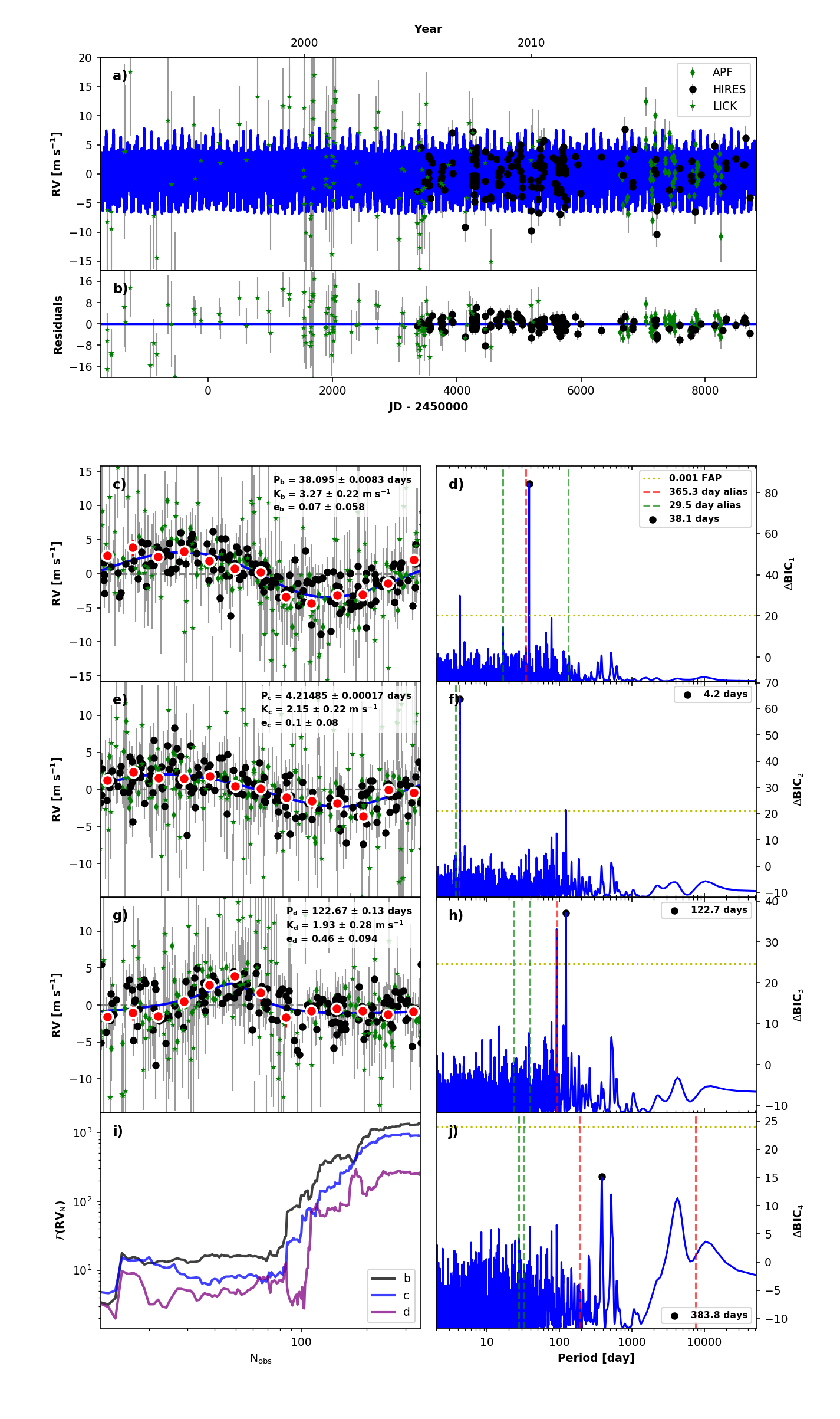
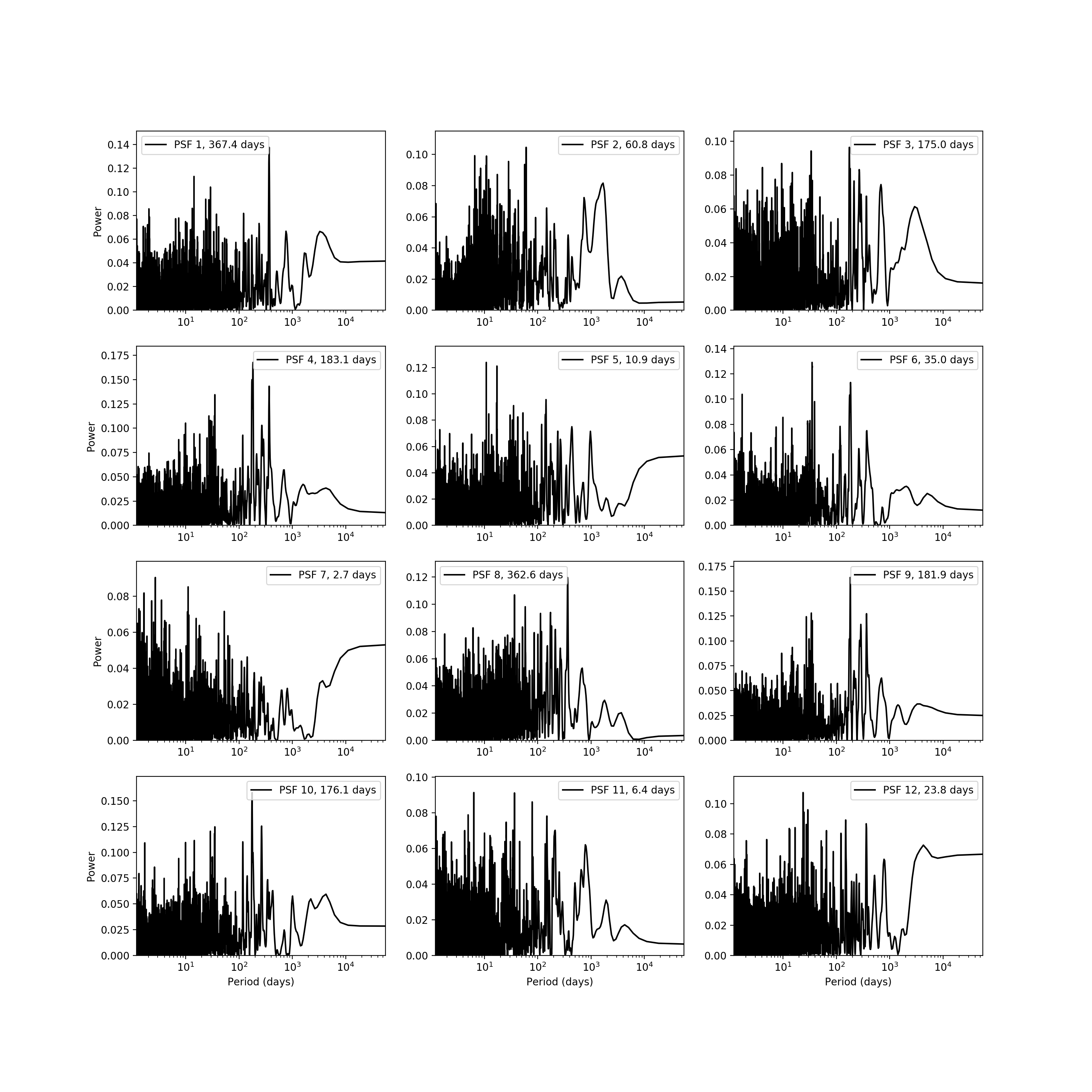
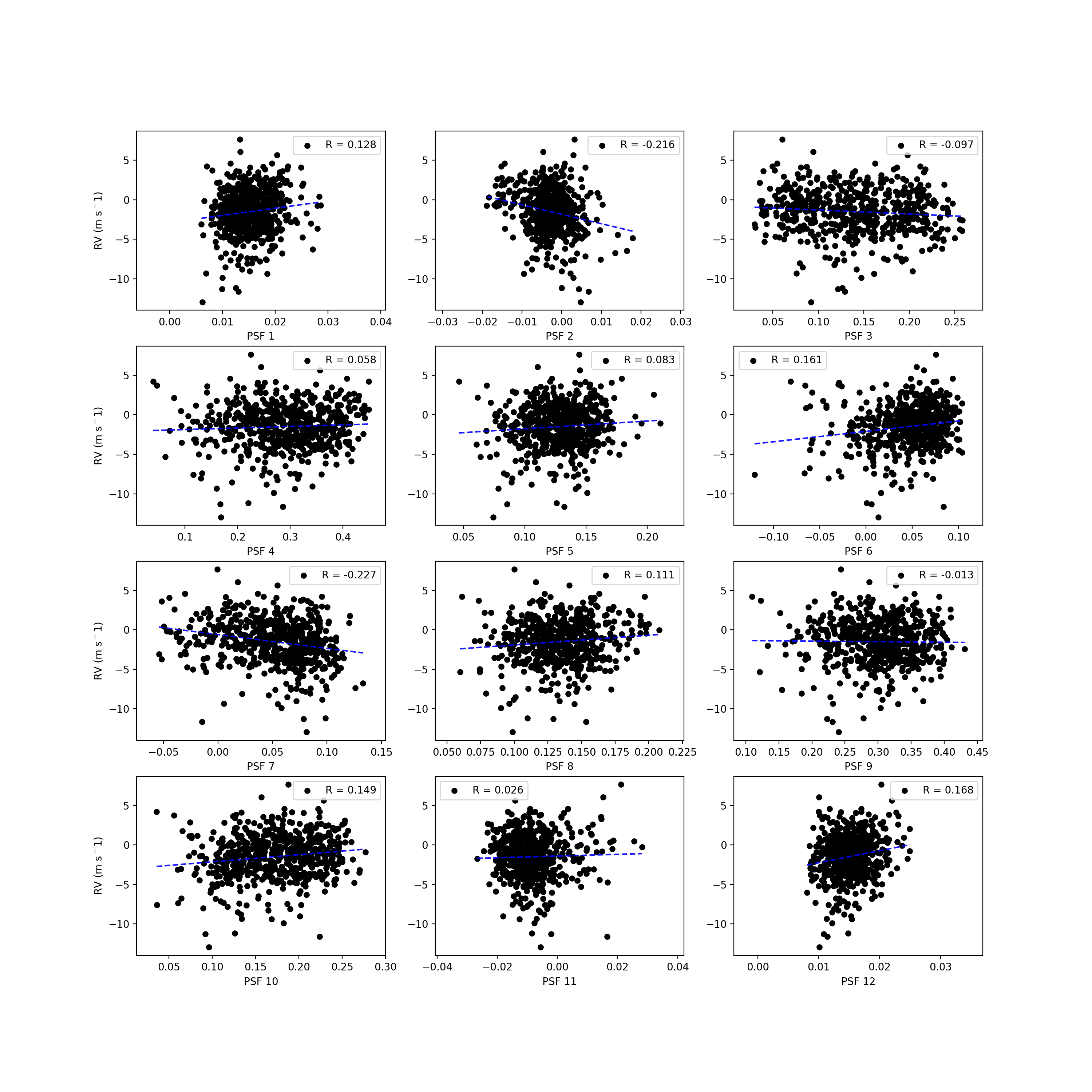
G.2 HD 154345

Here, we confirm the planetary status of the planet claim for HD 154345. Wright et al. (2008) announced the detection of a true Jupiter analog, with $M\sin{i}$ = 0.95 $M_{\textrm{J}}$ and an orbital period of 9.2 yr, corresponding to an orbital separation of 4.2 AU. This paper also presented strong evidence for a stellar magnetic activity cycle with a periodic timescale of roughly nine years. As the CPS group continued to observe HD 154345 over the next few years, the planet candidate’s RV signature and the corresponding S-values appeared to be strongly in phase, and Wright (2016) noted that the candidate may be a false positive. However, in the twelve years since HD 154345 b was initially reported, HIRES RV measurements and activity metrics have drifted from being completely in phase to being completely out of phase, as seen in Figure 46, and therefore are not linearly correlated. This strongly implies that this Jupiter analog candidate cannot be attributed to stellar activity, and that this candidate should be cemented as a confirmed planet. RVSearch detects two signals in our HD 154345 dataset, both close to 9 yr, as seen in Figure 47. We attribute the circular orbit with a greater RV amplitude to HD 154345 b, and the weak, eccentric signal to stellar activity.

Figure 46: HIRES post-upgrade RV and S-value activity timeseries for HD 154345. Note that the two datasets share minima and appear to be in phase when post-upgrade observations began, but have drifted completely out of phase over the following 23 years.

Figure 47: RVSearch summary plot for HD 154345; see Figure 6 for description. RVSearch first recovered a strong signal at  9 years, but then recovered additional power at a similar period due to stellar activity. The final orbit fit switched the two models, so that panels e) and d) show the planetary signal, while panels c) and f) show the stellar activity signal.

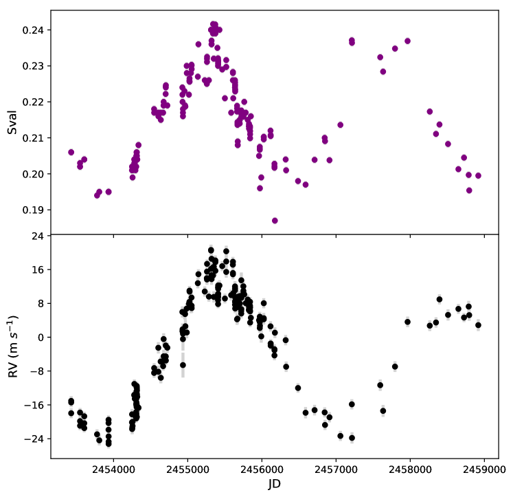
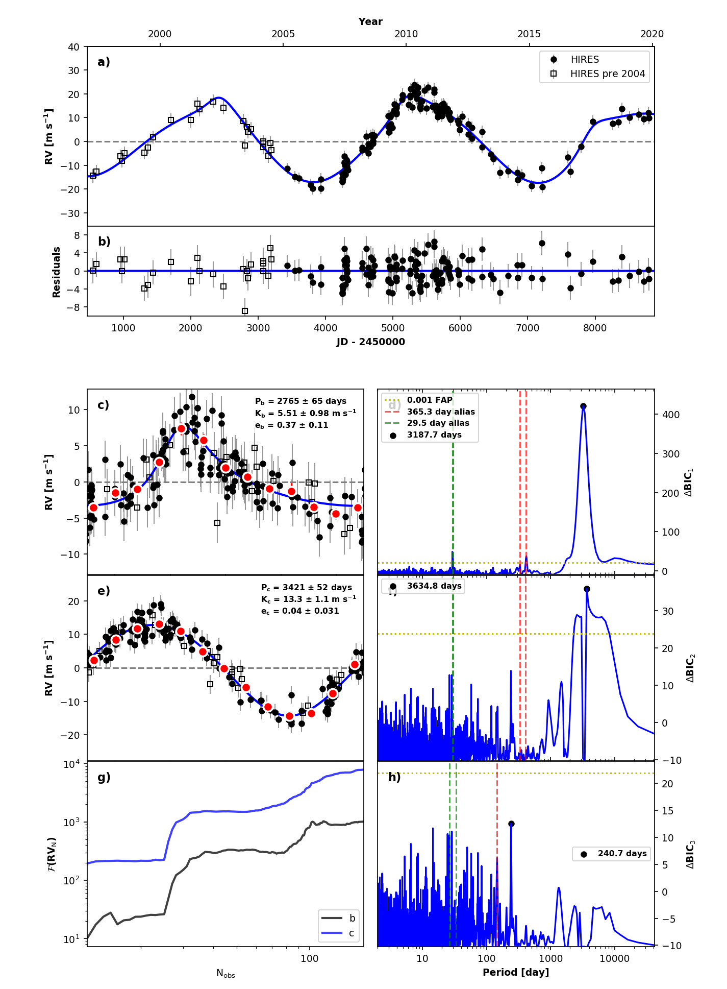
G.3 HD 26965

Ma et al. (2018) reported a 42.4 day super-Earth orbiting the nearby star HD 26965, using datasets taken by multiple spectrographs, including HIRES. We detected significant periodicity at 42 days in the HIRES S-value measurements as seen in Figure 48, and determined that 42 days is the likely stellar rotation period of HD 26965. There is also evidence of a long-period magnetic activity cycle, as seen in the juxtaposition of S-values and RVs in Figure 49.

Figure 48: Stellar rotation analysis of HIRES S-values for HD 26965. The top panel shows a Lomb–Scargle periodogram of the S-values after we applied a high-pass filter to them, to remove the impact of the long-period magnetic activity cycle. The middle panel shows a periodogram of the raw S-values. The top panel shows significant periodicity near 40 days, with a maximum at 41.6 days. The bottom-left panel shows the filtered S-values, while the bottom-right panel shows the filtered S-values phased to 41.6 days; there appears to be a coherent signal at this period, implying stellar rotation with this period.

Figure 49: HIRES post-upgrade S-values and RVs for HD 26965. The two datasets both have long-period power and are in phase with each other.

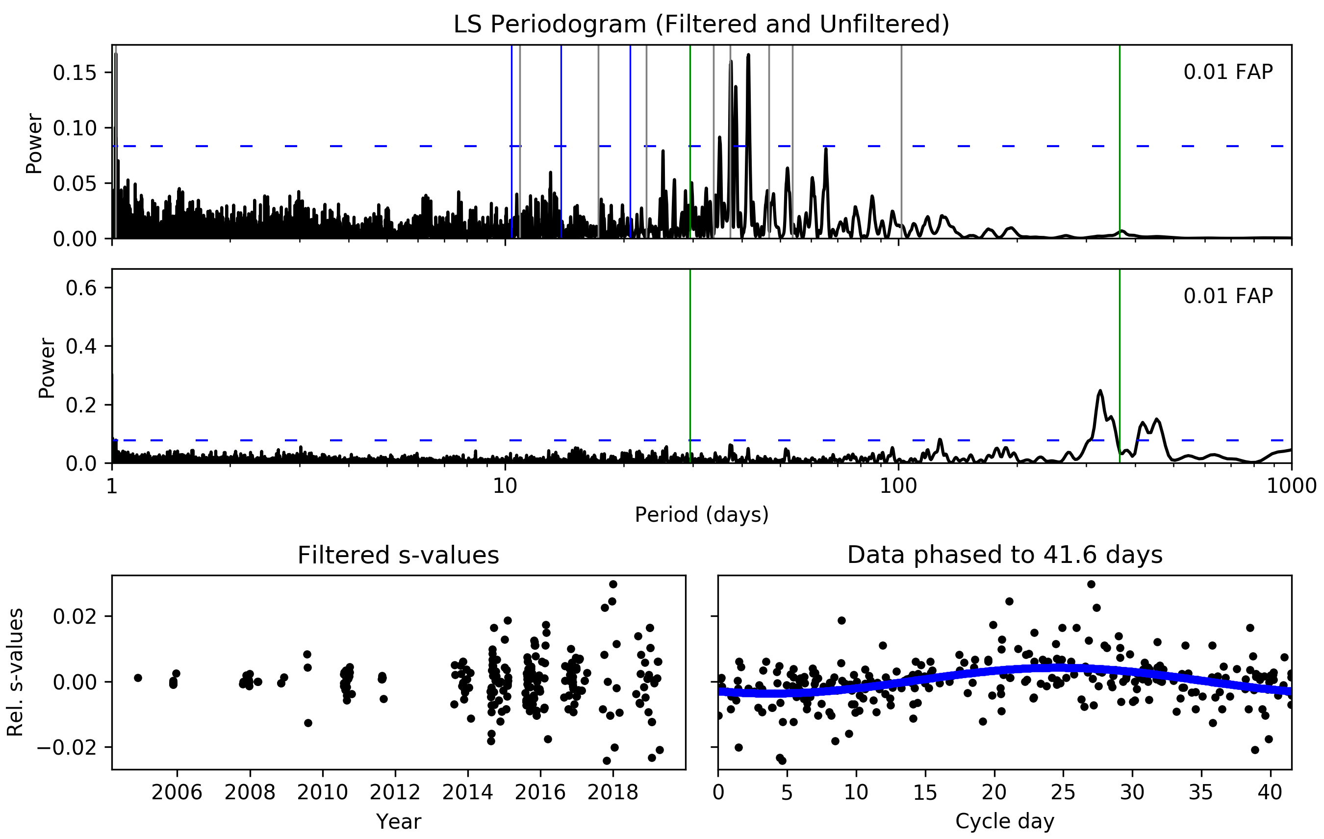
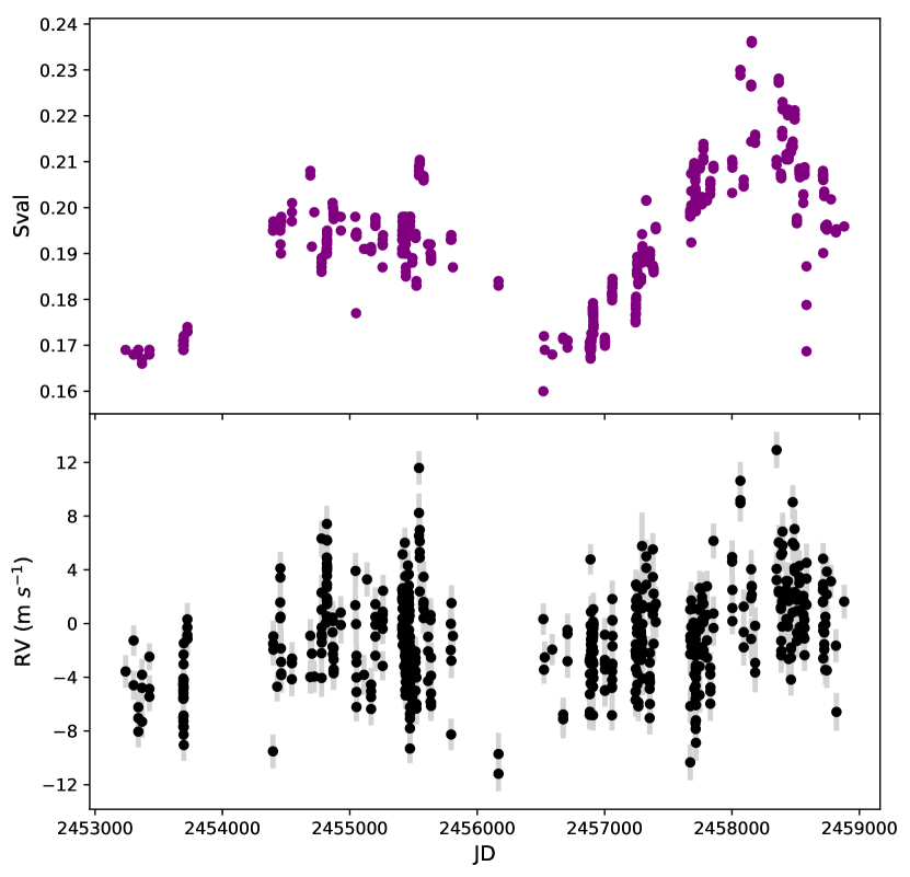
G.4 HD 34445

Howard et al. (2010a) reported a giant planet orbiting this star at a period of 1049 days. Vogt et al. (2017) reported five small planets, claiming evidence in LCES-derived HIRES radial velocities. RVSearch detected the giant planet and three of the five small planet claims, as seen in the summary plot shown in Figure 50. The longest-period candidate among the five, not modeled as a Keplerian here, clearly correlates with HIRES S-values; we model this signal with a linear trend, for simplicity. Figure 51 juxtaposes the HIRES S-values and corresponding RVs, minus the Keplerian signal of the system’s giant planet. As for the three other periodic signals that we detect, two are likely HIRES systematics and one is likely stellar rotation We detected significant periodicity at 52 days in the HIRES S-value measurements as seen in Figure 52, and determined that 52 days is the likely stellar rotation period of HD 34445. This places our weak detection of the 49 day claimed planet candidate under suspicion, and we have labeled it as a false positive in our catalog. There is also evidence of semiannual HIRES systematics, as seen in Figure 54, which shows the correlation between HIRES RVs minus the giant planet signature and PSF parameters, and in Figure 53, which shows periodograms of each PSF parameter time series. Multiple PSF parameters correlate ($|R|$ $>$ 0.15) with the RV residuals, and multiple parameters show periodicity around one-third and one-fourth of a year. The two claimed planets at 118 and 215 days are close to one-third and one-half of a year, respectively, and show weak and equal-strength signatures in their RVSearch periodograms, as seen in Figure 50. Therefore, we have labeled these signals as false positives in our catalog.

Figure 50: RVSearch summary plot for HD 34445; see Figure 6 for description. RVSearch first recovered the known giant planet,

Figure 51: HIRES post-upgrade RV and S-value activity timeseries for HD 34445, with the giant planet RV model subtracted. Note that these two datasets share a negative long-term trend, which we believe accounts for the claimed 5,700-day planet in the system.

Figure 52: Stellar rotation analysis of HIRES S-values for HD 34445. The top panel shows a Lomb–Scargle periodogram of the S-values after we applied a high-pass filter to them, to remove the impact of the long-period magnetic activity cycle. The middle panel shows a periodogram of the raw S-values. The top panel shows significant periodicity around 52.1 days. The bottom-left panel shows the filtered S-values, while the bottom-right panel shows the filtered S-values phased to 52.1 days; there appears to be a coherent signal at this period, implying stellar rotation with this period. This led us to label the 49 day claimed planet as a false positive, since there is insufficient evidence to distinguish it from stellar rotation.

Figure 53: PSF Lomb–Scargle periodograms for HD 34445. Each panel corresponds to a Doppler code PSF fitting parameter.

Figure 54: PSF correlation plots for HD 34445, without the RV signature of the star’s giant planet. Each panel corresponds to a Doppler code PSF fitting parameter, with PSF value on the x-axis and RV without the giant planet signature on the y-axis. Dashed blue lines are least-squares linear fits. R is the Pearson correlation value; multiple PSF parameters have $|R|$ $>$ 0.15.

References

- Alonso et al. (2004) Alonso, R., Brown, T. M., Torres, G., et al. 2004, ApJ, 613, L153
- Anglada-Escudé et al. (2012) Anglada-Escudé, G., Boss, A. P., Weinberger, A. J., et al. 2012, ApJ, 746, 37
- Apps et al. (2010) Apps, K., Clubb, K. I., Fischer, D. A., et al. 2010, PASP, 122, 156
- Bakos et al. (2002) Bakos, G. Á., Lázár, J., Papp, I., Sári, P., & Green, E. M. 2002, PASP, 114, 974
- Benatti et al. (2020) Benatti, S., Damasso, M., Desidera, S., et al. 2020, A&A, 639, A50
- Blunt et al. (2019) Blunt, S., Endl, M., Weiss, L. M., et al. 2019, AJ, 158, 181
- Boisse et al. (2012) Boisse, I., Pepe, F., Perrier, C., et al. 2012, A&A, 545, A55
- Bonfils et al. (2005) Bonfils, X., Forveille, T., Delfosse, X., et al. 2005, A&A, 443, L15
- Borucki (2016) Borucki, W. J. 2016, Reports on Progress in Physics, 79, 036901
- Boss (1997) Boss, A. P. 1997, Science, 276, 1836
- Bouchy et al. (2005) Bouchy, F., Udry, S., Mayor, M., et al. 2005, A&A, 444, L15
- Bowler et al. (2020) Bowler, B. P., Blunt, S. C., & Nielsen, E. L. 2020, AJ, 159, 63
- Bryan et al. (2019) Bryan, M. L., Knutson, H. A., Lee, E. J., et al. 2019, AJ, 157, 52
- Bryan et al. (2016) Bryan, M. L., Knutson, H. A., Howard, A. W., et al. 2016, ApJ, 821, 89
- Buchner (2016) Buchner, J. 2016, PyMultiNest: Python interface for MultiNest, , , ascl:1606.005
- Burt et al. (2014) Burt, J., Vogt, S. S., Butler, R. P., et al. 2014, ApJ, 789, 114
- Butler et al. (2006a) Butler, R. P., Johnson, J. A., Marcy, G. W., et al. 2006a, PASP, 118, 1685
- Butler & Marcy (1996) Butler, R. P., & Marcy, G. W. 1996, ApJ, 464, L153
- Butler et al. (1999) Butler, R. P., Marcy, G. W., Fischer, D. A., et al. 1999, ApJ, 526, 916
- Butler et al. (1998) Butler, R. P., Marcy, G. W., Vogt, S. S., & Apps, K. 1998, PASP, 110, 1389
- Butler et al. (2003) Butler, R. P., Marcy, G. W., Vogt, S. S., et al. 2003, ApJ, 582, 455
- Butler et al. (1997) Butler, R. P., Marcy, G. W., Williams, E., Hauser, H., & Shirts, P. 1997, ApJ, 474, L115
- Butler et al. (1996) Butler, R. P., Marcy, G. W., Williams, E., et al. 1996, PASP, 108, 500
- Butler et al. (2000) Butler, R. P., Vogt, S. S., Marcy, G. W., et al. 2000, ApJ, 545, 504
- Butler et al. (2004) —. 2004, ApJ, 617, 580
- Butler et al. (2002) Butler, R. P., Marcy, G. W., Vogt, S. S., et al. 2002, ApJ, 578, 565
- Butler et al. (2006b) Butler, R. P., Wright, J. T., Marcy, G. W., et al. 2006b, ApJ, 646, 505
- Butler et al. (2017) Butler, R. P., Vogt, S. S., Laughlin, G., et al. 2017, AJ, 153, 208
- Cochran et al. (1997) Cochran, W. D., Hatzes, A. P., Butler, R. P., & Marcy, G. W. 1997, ApJ, 483, 457
- Cumming et al. (2008) Cumming, A., Butler, R. P., Marcy, G. W., et al. 2008, PASP, 120, 531
- Dawson & Murray-Clay (2013) Dawson, R. I., & Murray-Clay, R. A. 2013, ApJ, 767, L24
- Díaz et al. (2012) Díaz, R. F., Santerne, A., Sahlmann, J., et al. 2012, A&A, 538, A113
- Díaz et al. (2019) Díaz, R. F., Delfosse, X., Hobson, M. J., et al. 2019, A&A, 625, A17
- Eaton et al. (2003) Eaton, J. A., Henry, G. W., & Fekel, F. C. 2003, in Astrophysics and Space Science Library, Vol. 288, Astrophysics and Space Science Library, ed. T. D. Oswalt, 189
- Feng et al. (2015) Feng, Y. K., Wright, J. T., Nelson, B., et al. 2015, ApJ, 800, 22
- Fernandes et al. (2019) Fernandes, R. B., Mulders, G. D., Pascucci, I., Mordasini, C., & Emsenhuber, A. 2019, ApJ, 874, 81
- Fischer et al. (2009) Fischer, D., Driscoll, P., Isaacson, H., et al. 2009, ApJ, 703, 1545
- Fischer et al. (2003) Fischer, D. A., Butler, R. P., Marcy, G. W., Vogt, S. S., & Henry, G. W. 2003, ApJ, 590, 1081
- Fischer et al. (1999) Fischer, D. A., Marcy, G. W., Butler, R. P., Vogt, S. S., & Apps, K. 1999, PASP, 111, 50
- Fischer et al. (2001) Fischer, D. A., Marcy, G. W., Butler, R. P., et al. 2001, ApJ, 551, 1107
- Fischer et al. (2002) —. 2002, PASP, 114, 529
- Fischer et al. (2014) Fischer, D. A., Marcy, G. W., & Spronck, J. F. P. 2014, ApJS, 210, 5
- Fischer et al. (2005) Fischer, D. A., Laughlin, G., Butler, P., et al. 2005, ApJ, 620, 481
- Fischer et al. (2007) Fischer, D. A., Vogt, S. S., Marcy, G. W., et al. 2007, ApJ, 669, 1336
- Fischer et al. (2008) Fischer, D. A., Marcy, G. W., Butler, R. P., et al. 2008, ApJ, 675, 790
- Foreman-Mackey et al. (2013) Foreman-Mackey, D., Hogg, D. W., Lang, D., & Goodman, J. 2013, PASP, 125, 306
- Forveille et al. (2009) Forveille, T., Bonfils, X., Delfosse, X., et al. 2009, A&A, 493, 645
- Fulton (2017) Fulton, B. J. 2017, PhD thesis, University of Hawai’i at Manoa
- Fulton et al. (2018) Fulton, B. J., Petigura, E. A., Blunt, S., & Sinukoff, E. 2018, PASP, 130, 044504
- Fulton et al. (2015) Fulton, B. J., Weiss, L. M., Sinukoff, E., et al. 2015, ApJ, 805, 175
- Fulton et al. (2016) Fulton, B. J., Howard, A. W., Weiss, L. M., et al. 2016, ApJ, 830, 46
- Gaia Collaboration et al. (2016) Gaia Collaboration, Brown, A. G. A., Vallenari, A., et al. 2016, A&A, 595, A2
- Gaia Collaboration et al. (2018) —. 2018, A&A, 616, A1
- Gonzalez (1997) Gonzalez, G. 1997, MNRAS, 285, 403
- Gregory & Fischer (2010) Gregory, P. C., & Fischer, D. A. 2010, MNRAS, 403, 731
- Haghighipour et al. (2010) Haghighipour, N., Vogt, S. S., Butler, R. P., et al. 2010, ApJ, 715, 271
- Hatzes et al. (2000) Hatzes, A. P., Cochran, W. D., McArthur, B., et al. 2000, ApJ, 544, L145
- Haywood et al. (2014) Haywood, R. D., Collier Cameron, A., Queloz, D., et al. 2014, MNRAS, 443, 2517
- Henry (1999) Henry, G. W. 1999, PASP, 111, 845
- Henry et al. (2000) Henry, G. W., Marcy, G. W., Butler, R. P., & Vogt, S. S. 2000, ApJ, 529, L41
- Henry et al. (2013) Henry, G. W., Kane, S. R., Wang, S. X., et al. 2013, ApJ, 768, 155
- Hillenbrand et al. (2015) Hillenbrand, L., Isaacson, H., Marcy, G., et al. 2015, in Cambridge Workshop on Cool Stars, Stellar Systems, and the Sun, Vol. 18, 18th Cambridge Workshop on Cool Stars, Stellar Systems, and the Sun, 759–766
- Hirsch et al. (2020) Hirsch, L. A., Rosenthal, L., Fulton, B. J., et al. 2020, arXiv e-prints, arXiv:2012.09190
- Horne & Baliunas (1986) Horne, J. H., & Baliunas, S. L. 1986, ApJ, 302, 757
- Howard & Fulton (2016) Howard, A. W., & Fulton, B. J. 2016, PASP, 128, 114401
- Howard et al. (2010a) Howard, A. W., Johnson, J. A., Marcy, G. W., et al. 2010a, ApJ, 721, 1467
- Howard et al. (2010b) Howard, A. W., Marcy, G. W., Johnson, J. A., et al. 2010b, Science, 330, 653
- Howard et al. (2011) Howard, A. W., Johnson, J. A., Marcy, G. W., et al. 2011, ApJ, 726, 73
- Howard et al. (2014) Howard, A. W., Marcy, G. W., Fischer, D. A., et al. 2014, ApJ, 794, 51
- Huber (2017) Huber, D. 2017, Isoclassify: V1.2, vv1.2, Zenodo, doi:10.5281/zenodo.573372
- Isaacson & Fischer (2010) Isaacson, H., & Fischer, D. 2010, ApJ, 725, 875
- Johnson et al. (2010a) Johnson, J. A., Aller, K. M., Howard, A. W., & Crepp, J. R. 2010a, PASP, 122, 905
- Johnson et al. (2007a) Johnson, J. A., Butler, R. P., Marcy, G. W., et al. 2007a, ApJ, 670, 833
- Johnson et al. (2008) Johnson, J. A., Marcy, G. W., Fischer, D. A., et al. 2008, ApJ, 675, 784
- Johnson et al. (2007b) Johnson, J. A., Fischer, D. A., Marcy, G. W., et al. 2007b, ApJ, 665, 785
- Johnson et al. (2010b) Johnson, J. A., Bowler, B. P., Howard, A. W., et al. 2010b, ApJ, 721, L153
- Johnson et al. (2017) Johnson, J. A., Petigura, E. A., Fulton, B. J., et al. 2017, AJ, 154, 108
- Jones et al. (2010) Jones, H. R. A., Butler, R. P., Tinney, C. G., et al. 2010, MNRAS, 403, 1703
- Kane et al. (2014) Kane, S. R., Howell, S. B., Horch, E. P., et al. 2014, ApJ, 785, 93
- Kipping (2013) Kipping, D. M. 2013, MNRAS, 434, L51
- Knutson et al. (2014) Knutson, H. A., Fulton, B. J., Montet, B. T., et al. 2014, ApJ, 785, 126
- Lindegren et al. (2018) Lindegren, L., Hernández, J., Bombrun, A., et al. 2018, A&A, 616, A2
- Lockwood et al. (2013) Lockwood, G. W., Henry, G. W., Hall, J. C., & Radick, R. R. 2013, Astronomical Society of the Pacific Conference Series, Vol. 472, Decadal Variations of Sun-Like Stars, ed. M. Chavez, E. Bertone, O. Vega, & V. De la Luz, 203
- Lovis et al. (2006) Lovis, C., Mayor, M., Pepe, F., et al. 2006, Nature, 441, 305
- Lucy & Sweeney (1971) Lucy, L. B., & Sweeney, M. A. 1971, AJ, 76, 544
- Ma et al. (2018) Ma, B., Ge, J., Muterspaugh, M., et al. 2018, MNRAS, 480, 2411
- Marcy et al. (2001) Marcy, G. W., Butler, R. P., Fischer, D., et al. 2001, ApJ, 556, 296
- Marcy et al. (2002) Marcy, G. W., Butler, R. P., Fischer, D. A., et al. 2002, ApJ, 581, 1375
- Marcy et al. (2000) Marcy, G. W., Butler, R. P., & Vogt, S. S. 2000, ApJ, 536, L43
- Marcy et al. (1998) Marcy, G. W., Butler, R. P., Vogt, S. S., Fischer, D., & Lissauer, J. J. 1998, ApJ, 505, L147
- Marcy et al. (1999) Marcy, G. W., Butler, R. P., Vogt, S. S., Fischer, D., & Liu, M. C. 1999, ApJ, 520, 239
- Marcy et al. (2005) Marcy, G. W., Butler, R. P., Vogt, S. S., et al. 2005, ApJ, 619, 570
- Mayor & Queloz (1995) Mayor, M., & Queloz, D. 1995, Nature, 378, 355
- Mayor et al. (2004) Mayor, M., Udry, S., Naef, D., et al. 2004, A&A, 415, 391
- Mayor et al. (2009) Mayor, M., Bonfils, X., Forveille, T., et al. 2009, A&A, 507, 487
- Mayor et al. (2011) Mayor, M., Marmier, M., Lovis, C., et al. 2011, arXiv e-prints, arXiv:1109.2497
- McArthur et al. (2004) McArthur, B. E., Endl, M., Cochran, W. D., et al. 2004, ApJ, 614, L81
- McKinney (2010) McKinney, W. 2010, in Proceedings of the 9th Python in Science Conference, ed. S. van der Walt & J. Millman, 51 – 56
- Meschiari et al. (2011) Meschiari, S., Laughlin, G., Vogt, S. S., et al. 2011, ApJ, 727, 117
- Mordasini et al. (2011) Mordasini, C., Mayor, M., Udry, S., et al. 2011, A&A, 526, A111
- Naef et al. (2004) Naef, D., Mayor, M., Beuzit, J. L., et al. 2004, VizieR Online Data Catalog, J/A+A/414/351
- Naef et al. (2001) Naef, D., Mayor, M., Pepe, F., et al. 2001, A&A, 375, 205
- Naef et al. (2003) Naef, D., Mayor, M., Korzennik, S. G., et al. 2003, A&A, 410, 1051
- Nielsen et al. (2019) Nielsen, E. L., De Rosa, R. J., Macintosh, B., et al. 2019, AJ, 158, 13
- Noyes et al. (1997) Noyes, R. W., Jha, S., Korzennik, S. G., et al. 1997, ApJ, 483, L111
- Pepe et al. (2002) Pepe, F., Mayor, M., Galland, F., et al. 2002, A&A, 388, 632
- Pepper (2007) Pepper, J. 2007, PhD thesis, The Ohio State University
- Perrier et al. (2003) Perrier, C., Sivan, J. P., Naef, D., et al. 2003, A&A, 410, 1039
- Petigura (2015) Petigura, E. A. 2015, PhD thesis, University of California, Berkeley
- Pollacco et al. (2006) Pollacco, D. L., Skillen, I., Collier Cameron, A., et al. 2006, PASP, 118, 1407
- Pollack et al. (1996) Pollack, J. B., Hubickyj, O., Bodenheimer, P., et al. 1996, Icarus, 124, 62
- Price-Whelan et al. (2017) Price-Whelan, A. M., Hogg, D. W., Foreman-Mackey, D., & Rix, H.-W. 2017, ApJ, 837, 20
- Radovan et al. (2014) Radovan, M. V., Lanclos, K., Holden, B. P., et al. 2014, Society of Photo-Optical Instrumentation Engineers (SPIE) Conference Series, Vol. 9145, The automated planet finder at Lick Observatory, 91452B
- Reiners et al. (2018) Reiners, A., Ribas, I., Zechmeister, M., et al. 2018, A&A, 609, L5
- Rickman et al. (2019) Rickman, E. L., Ségransan, D., Marmier, M., et al. 2019, A&A, 625, A71
- Rivera et al. (2010) Rivera, E. J., Laughlin, G., Butler, R. P., et al. 2010, ApJ, 719, 890
- Roberts et al. (2011) Roberts, Lewis C., J., Turner, N. H., ten Brummelaar, T. A., Mason, B. D., & Hartkopf, W. I. 2011, AJ, 142, 175
- Robertson et al. (2014) Robertson, P., Mahadevan, S., Endl, M., & Roy, A. 2014, Science, 345, 440
- Rodigas et al. (2011) Rodigas, T. J., Males, J. R., Hinz, P. M., Mamajek, E. E., & Knox, R. P. 2011, ApJ, 732, 10
- Rowan et al. (2016) Rowan, D., Meschiari, S., Laughlin, G., et al. 2016, ApJ, 817, 104
- Santos et al. (2001) Santos, N. C., Mayor, M., Naef, D., et al. 2001, A&A, 379, 999
- Santos et al. (2000) —. 2000, A&A, 356, 599
- Tal-Or et al. (2019) Tal-Or, L., Trifonov, T., Zucker, S., Mazeh, T., & Zechmeister, M. 2019, MNRAS, 484, L8
- Tange (2011) Tange, O. 2011, ;login: The USENIX Magazine, 36, 42. http://www.gnu.org/s/parallel
- Tinney et al. (2001) Tinney, C. G., Butler, R. P., Marcy, G. W., et al. 2001, ApJ, 551, 507
- Trifonov et al. (2018) Trifonov, T., Kürster, M., Zechmeister, M., et al. 2018, A&A, 609, A117
- Udry et al. (2000) Udry, S., Mayor, M., Naef, D., et al. 2000, A&A, 356, 590
- Udry et al. (2019) Udry, S., Dumusque, X., Lovis, C., et al. 2019, A&A, 622, A37
- Valenti et al. (1995) Valenti, J. A., Butler, R. P., & Marcy, G. W. 1995, PASP, 107, 966
- van der Walt et al. (2011) van der Walt, S., Colbert, S. C., & Varoquaux, G. 2011, Computing in Science Engineering, 13, 22
- Vogt et al. (2005) Vogt, S. S., Butler, R. P., Marcy, G. W., et al. 2005, ApJ, 632, 638
- Vogt et al. (2002) —. 2002, ApJ, 568, 352
- Vogt et al. (2000) Vogt, S. S., Marcy, G. W., Butler, R. P., & Apps, K. 2000, ApJ, 536, 902
- Vogt et al. (1994) Vogt, S. S., Allen, S. L., Bigelow, B. C., et al. 1994, Society of Photo-Optical Instrumentation Engineers (SPIE) Conference Series, Vol. 2198, HIRES: the high-resolution echelle spectrometer on the Keck 10-m Telescope, ed. D. L. Crawford & E. R. Craine, 362
- Vogt et al. (2010) Vogt, S. S., Wittenmyer, R. A., Butler, R. P., et al. 2010, ApJ, 708, 1366
- Vogt et al. (2014) Vogt, S. S., Radovan, M., Kibrick, R., et al. 2014, PASP, 126, 359
- Vogt et al. (2015) Vogt, S. S., Burt, J., Meschiari, S., et al. 2015, ApJ, 814, 12
- Vogt et al. (2017) Vogt, S. S., Butler, R. P., Burt, J., et al. 2017, AJ, 154, 181
- Wittenmyer et al. (2007a) Wittenmyer, R. A., Endl, M., & Cochran, W. D. 2007a, ApJ, 654, 625
- Wittenmyer et al. (2007b) Wittenmyer, R. A., Endl, M., Cochran, W. D., & Levison, H. F. 2007b, AJ, 134, 1276
- Wittenmyer et al. (2020) Wittenmyer, R. A., Wang, S., Horner, J., et al. 2020, MNRAS, 492, 377
- Wittrock et al. (2017) Wittrock, J. M., Kane, S. R., Horch, E. P., et al. 2017, AJ, 154, 184
- Wright (2016) Wright, J. T. 2016, arXiv e-prints, arXiv:1603.08384
- Wright et al. (2008) Wright, J. T., Marcy, G. W., Butler, R. P., et al. 2008, ApJ, 683, L63
- Wright et al. (2009) Wright, J. T., Upadhyay, S., Marcy, G. W., et al. 2009, ApJ, 693, 1084
- Wright et al. (2007) Wright, J. T., Marcy, G. W., Fischer, D. A., et al. 2007, ApJ, 657, 533
- Yee et al. (2017) Yee, S. W., Petigura, E. A., & von Braun, K. 2017, ApJ, 836, 77
- Zhu & Wu (2018) Zhu, W., & Wu, Y. 2018, AJ, 156, 92
- Zucker et al. (2002) Zucker, S., Naef, D., Latham, D. W., et al. 2002, ApJ, 568, 363