NPD Entropy: A Non-Parametric Differential Entropy Rate Estimator

Abstract

The estimation of entropy rates for stationary discrete-valued stochastic processes is a well studied problem in information theory. However, estimating the entropy rate for stationary continuous-valued stochastic processes has not received as much attention. In fact, many current techniques are not able to accurately estimate or characterise the complexity of the differential entropy rate for strongly correlated processes, such as Fractional Gaussian Noise and ARFIMA(0,d,0). To the point that some cannot even detect the trend of the entropy rate, e.g., when it increases/decreases, maximum, or asymptotic trends, as a function of their Hurst parameter. However, a recently developed technique provides accurate estimates at a high computational cost. In this paper, we define a robust technique for non-parametrically estimating the differential entropy rate of a continuous valued stochastic process from observed data, by making an explicit link between the differential entropy rate and the Shannon entropy rate of a quantised version of the original data. Estimation is performed by a Shannon entropy rate estimator, and then converted to a differential entropy rate estimate. We show that this technique inherits many important statistical properties from the Shannon entropy rate estimator. The estimator is able to provide better estimates than the defined relative measures and much quicker estimates than known absolute measures, for strongly correlated processes. Finally, we analyse the complexity of the estimation technique and test the robustness to non-stationarity, and show that none of the current techniques are robust to non-stationarity, even if they are robust to strong correlations.

I Introduction

Estimation of entropy rate is a classical problem in information theory. The entropy rate is the asymptotic limit of the average per sample entropy of a discrete-time stationary stochastic process. It is used as a measure of the complexity of the process and thus to perform comparisons.

Estimation of entropy rate is easy when the underlying stochastic process is known to follow a simple model such as a Markov chain. The reality is that most real data sequences are not trivial to model. Non-parametric approaches to estimation have the very significant advantage that they do not depend on a fitting a model of the data and hence have a degree of robustness missing from parametric estimators.

A great deal of theory has been developed on non-parametric entropy rate estimation from data from finite alphabets [21, 32], since these models form the basis of discrete codes for communications. These estimation techniques have been extended to countably infinite alphabets [28, 20]. However, these approaches cannot be directly applied to continuous-valued stochastic processes, which are the main topic of interest here.

There are approaches that have been designed for estimating the complexity of continuous-valued stochastic processes: approximate [27], sample [30] and permutation entropy [2]. These estimators have been used in estimating the entropy rate for processes, particularly for those that are memoryless or have short memory. For example, approximate entropy has been shown to converge to the entropy rate for independent and identically distributed processes and first order Markov chains in the discrete-valued case [27]. However, at best, these estimators are sensitive to their parameter choices; at worst we shall see that they have severe defects.

In this paper, we compare the existing approaches and develop a new non-parametric differential entropy rate estimator – NPD Entropy – for continuous-valued stochastic processes. It combines the best of the existing discrete alphabet non-parametric estimators with the standard signal processing techniques to obtain a estimate that is more reliable than the alternatives. We have implemented this estimator in Python as a package, npd_entropy, that is available on GitHub.

	Values		Estimation Quality				Computation
Estimation Technique	Discrete	Continuous	Consistent	Asymp. unbiased	Correlation Length	Complexity	Time (s)
Grassberger [16]	✔	✖	✖	✖	$\approx\log(N)$
Kontoyiannis and Suhov [21]	✔	✖	✔	✔	$\approx\log(N)$
Approximate Entropy [27]	✔	✔	✖	✖	$m$	$O(N^{2})$	$10.01$
Sample Entropy [30]	✔	✔	✖	✖	$m$	$O(N^{2})$	$263.0$
Permutation Entropy [2]	✔	✔	✖	✖	$n$	$O(n!N)$	$0.82$
Specific Entropy [8]	✖	✔	✔	✔	$p$	$O(N^{2}p)$	$504,219.9$
NPD Entropy	✖	✔	✔	✔	$\approx\log(N)$	$O(N\log N)$	$39.96$

Table I: Comparison of entropy rate estimators. The estimator from Kontoyiannis and Suhov has desirable properties: consistent and asymptotically unbiased. Approximate, sample and permutation entropy can be applied to either discrete or continuous valued sequences but these are biased and inconsistent. Correlation length refers to the longest lag at which correlations are included into the entropy rate estimate where the length of data is $N$, the length of substrings matched in approximate and sample entropy is $m$, the order of permutations used in permutation entropy is $n$, and $p$ is the number of previous observations used in the conditional entropy calculation. Note also that although specific entropy behaves relatively well, its computation times are prohibitive. We have only included the complexity and computation time for the continuous-valued estimators that we test in this paper.

Table I outlines our results. Notably, some discrete estimators are consistent and asymptotic unbiased, but cannot be applied directly to continuous-valued processes as they are based on string matching. On the other hand, the main approaches that have been applied to continuous values – approximate, sample and permutation entropy – are not consistent, and use (short) finite windows, limiting their ability to cope with processes with extended correlations. We show, for instance, that these estimation techniques do not make accurate estimates for the entropy rate for processes whose dependency structure has slowly decaying correlations.

We examine these entropy rate estimates performance on data generated by long range dependent (LRD) processes. LRD processes have been shown to be effective models for phenomena such as network traffic [24, 34], finance [35], climate science [33] and hydrology [19]. We apply the estimation approaches to two common LRD processes with known entropy rate properites. Thus we can show exactly how bad some estimators are when applied to an even slightly challenging data set.

Another alternative – specific entropy – was developed as a technique to calculate the predictive uncertainty for a specific state of a continuous-valued process [8]. This approach utilises more rigorous statistical foundations to estimate the entropy rate of a state given the observation of a finite past. The technique is able to make accurate entropy rate estimates by calculating the average over the states and is able to capture the complex dependency structure with past observations. However this comes at a large computational cost, and hence cannot be used for large sequences, or for streaming data to make online estimates (see Table I for computation time comparisons).

We develop an estimation technique – NPD Entropy – that utilises discrete state non-parametric estimators. We utilise a connection between the Shannon entropy and differential entropy [6, pg. 248], and then extend it to the case of entropy rates. The technique quantises the continuous-valued data into discrete bins, then makes an estimation of the quantised process using discrete alphabet techniques. Then the differential entropy rate estimate is calculated by adjusting by the quantitative difference between the differential entropy rate and the Shannon entropy rate of the quantised process.

We show that NPD Entropy inherits useful estimation properties from discrete alphabet estimators. Hence, by choosing a discrete estimator with the desired properties we can ensure that NPD Entropy has the same properties for estimation on continuous-valued data. We show that this performs well in the estimation of differential entropy rate of stochastic processes which have more complex dependency structure.

We also compare the runtime performance of techniques and find that NPD Entropy can make much faster estimates than any approach of comparable accuracy.

II Background

II-A Entropy Rate

In this section we’ll define the concepts required. Many of these are standard, but we define them carefully here because of the proliferation of terms involving “entropy” in some manner. First we’ll define the Shannon entropy of a discrete random variable. This is the classic definition of information entropy from Claude Shannon’s foundational paper [31].

Definition II.1.

For a discrete random variable, $X$, with support on $\Omega$, and a probability mass function $p(x)$, the Shannon entropy, $H(X)$ is defined as, $H(X)=-\sum_{x\in\Omega}p(x)\log p(x).$

We extend the definition of Shannon entropy for a collection of random variables, called the joint entropy.

Definition II.2.

For a collection of discrete random variables, $X_{1},...,X_{n}$, with support on, $\Omega_{1},...,\Omega_{n}$ and joint probability mass function $p(x_{1},...,x_{n})=p(\mathbf{x})$, we define the joint entropy of the collection of random variables as,

$$H(X_{1},...,X_{n}) =-\sum_{x_{1}\in\Omega_{1}}...\sum_{x_{n}\in\Omega_{n}}p(\mathbf{x})\log p(\mathbf{x}).$$

Entropy can be thought of as the average uncertainty or randomness contained in a random variable. We want an entropic notion that can be applied to stochastic processes, and hence we will define the entropy rate, the average uncertainty per random variable.

Definition II.3.

For a discrete-valued, discrete-time stochastic process, $\raisebox{0.0pt}{$\chi$}=\{X_{i}\}_{i\in\mathbb{N}}$, the entropy rate, is defined where the limit exists as,

$$H(\raisebox{0.0pt}{$\chi$}) =\lim\limits_{n\rightarrow\infty}\frac{1}{n}H(X_{1},...,X_{n}).$$

In this paper, we are considering the entropy rate of stochastic processes of continuous random variables, so we’ll need to extend the notion of entropy to continuous random variables. Claude Shannon in his original treatment of entropy [31], extended the definition by considering the definition of Shannon entropy as the expected value of the information content, i.e., $H(X)=-E[\log(p(X))]$.

Definition II.4.

The differential entropy, $h(X)$ of a random variable, $X$, with support, $\Omega$, and probability density function, $f(x)$, is,

$$h(X) =-\int_{\Omega}f(x)\log f(x)dx.$$

Differential entropy has some important properties which are different from Shannon entropy. For example, differential entropy can be negative, or even diverge to $-\infty$, which we can see by considering the Dirac delta function, $\delta(x)$, i.e., the unit impulse, defined by the properties $\delta(x)=0$ for $x\neq 0$ and $\int_{-\infty}^{\infty}\delta(x)\,dx=1$. The Dirac delta can be thought of in terms of probability as a completely determined point in time, that is, a function possessing no uncertainty. It can be constructed as the limit of rectangular pulses of constant area 1 as their width decreases, equivalent to the density of a uniform random variable, and hence we can calculate the entropy of the Dirac delta as

$$h(X)=-\int_{-a}^{a}\frac{1}{2a}\log\left(\frac{1}{2a}\right)dx=\log(2a),$$

which tends to $-\infty$ as $a\rightarrow 0$.

Similar to Shannon entropy we define the joint differential entropy for a collection of continuous random variables.

Definition II.5.

The joint differential entropy of a collection of continuous random variables, $X_{1},...,X_{n}$, with support on, $\Omega_{1}\times...\times\Omega_{n}$, with a joint density function, $f(x_{1},...,x_{n})=f(\mathbf{x})$, is

$$h(X_{1},...,X_{n}) =-\int_{\Omega_{1}}...\int_{\Omega_{n}}f(\mathbf{x})\log f(\mathbf{x})d\mathbf{x}.$$

Now we can define the object that we want to estimate, the differential entropy rate. This is a direct analogue of the discrete-valued random variable case.

Definition II.6.

The differential entropy rate for a continuous-valued, discrete-time stochastic process, $\raisebox{0.0pt}{$\chi$}=\{X_{i}\}_{i\in\mathbb{N}}$, is defined where the limit exists as,

$$h(\raisebox{0.0pt}{$\chi$}) =\lim\limits_{n\rightarrow\infty}\frac{1}{n}h(X_{1},...,X_{n}).$$

We state an equivalent characterisation of the differential entropy rate for stationary stochastic processes, using conditional entropy. This was developed for the Shannon entropy of discrete processes, however can be extended to differential entropy utilising an identical argument [6, pg. 416].

Theorem II.1.

For a stationary stochastic process, $\{X_{i}\}_{i\in\mathbb{N}}$, the differential entropy rate where the limit exists is equal to,

$$h(\raisebox{0.0pt}{$\chi$}) =\lim\limits_{n\rightarrow\infty}h(X_{n}|X_{n-1},...,X_{1}).$$

This states that the differential entropy rate is the limit of the new information that we get from each new random variable, after observing the infinite past.

II-B Strongly Correlated Processes

Now we will define the notion of a stochastic process with strong correlations, which we will use to test the effectiveness of the entropy rate estimation techniques. We will be using processes which are called long range dependent (LRD). In many contexts, e.g., [24, 34, 35, 33, 19], these processes are the norm, not pathologies. LRD processes have an autocorrelation function, $\rho(k)$, which decays as a power law in contrast to short-range correlated processes whose autocorrelations decay exponentially, and which have typically been used to test entropy estimators. However, LRD processes are still stationary, and can be modelled relatively simply, and thus form a practically useful test case, which should be seen as only mildly challenging.

Definition II.7.

Let $\{X_{n}\}_{n\in\mathbb{N}}$ be a stationary process. If there exists an $\alpha\in(0,1)$ and a constant $c_{\rho}>0$, such that,

$$\lim\limits_{k\rightarrow\infty}\frac{\rho(k)}{c_{\rho}k^{-\alpha}}=1.$$

Then we say that, $X_{n}$, is long range dependent.

An implication of this is that the sum of the autocorrelations diverges, i.e., $\sum_{k=1}^{\infty}c_{\rho}k^{-\alpha}=\infty$, which is often given as an equivalent definition of LRD [4, pg. 43].

A parameter of interest when analysing the strength of correlations is the Hurst parameter, $H$. It it linked to the exponent of the power-law decay by the relationship [4, pg. 42], $H=1-\alpha/2$. $H$ takes values between 0 and 1, with $H>\frac{1}{2}$ representing the region where the process is positively correlated, with the process becoming completely correlated at $H=1$. We call processes in this case LRD, otherwise we call them short range dependent (SRD). The region $H<\frac{1}{2}$ represents the region where a process is negatively correlated, with a completely negatively correlated process is at $H=0$. The autocorrelation functions sum to one in this case, $\sum_{k=1}^{\infty}\gamma(k)=0$, and is called constrained short range dependent (CSRD) [15]. This case much less studied, and the differential entropy rate differs between FGN and ARFIMA(0,d,0) [13]. Finally the mid point, $H=\frac{1}{2}$ are processes with short range or no correlations, i.e., white Gaussian noise.

II-B1 Fractional Gaussian Noise

Fractional Brownian Motion (FBM) is a continuous time Gaussian process, $B_{H}(t)$, on $[0,T]$, $B_{H}(0)=0$, $E[B_{H}(t)]=0,\forall t\in[0,T]$, and with covariance function,

$$E[B_{H}(t)B_{H}(s)] =\frac{1}{2}\left(t^{2H}+s^{2H}-|t-s|^{2H}\right),$$

where $H$ is the Hurst parameter [25]. Fractional Gaussian (FGN) Noise is the stationary increment process of FBM, i.e., $X(t)=B_{H}(t+1)-B_{H}(t)$.

The entropy rate of FGN is [13]

$$h(\raisebox{0.0pt}{$\chi$})=\frac{1}{2}\log(2\pi e)+\frac{1}{4\pi}\int_{-\pi}^{\pi}\log f(\lambda)d\lambda,$$

with the spectral density

$$f(\lambda)=2c_{f}(1-\cos\lambda)\sum_{j=-\infty}^{\infty}|2\pi j+\lambda|^{-2H-1},$$

where $c_{f}=\frac{\sigma^{2}}{2\pi}\sin\left(\pi H\right)\Gamma\left(2H+1\right)$. Here we calculate the integral numerically.

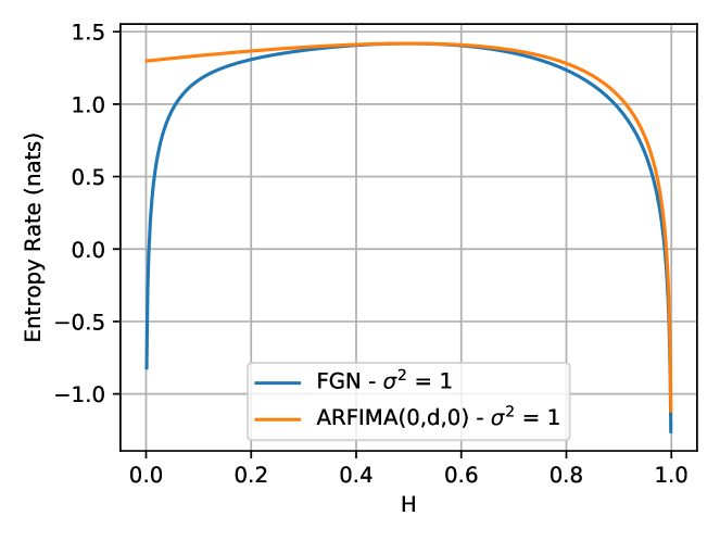
Figure 1: The entropy rate of FGN and ARFIMA(0,d,0) processes with variance, $\sigma^{2}=1$, as function of the Hurst parameter. The maximum for both processes is at $H=0.5$, and the function tends to $-\infty$ asymptotically as $H\rightarrow$ 0 and 1 for FGN and $H\rightarrow$ 1 only for ARFIMA(0,d,0)[13].

We plot the entropy rate of FGN as a function of the Hurst parameter in Figure 1. The entropy rate function attains a maximum at $H=0.5$, which is where the process is completely uncorrelated. As the process tends to 0 or 1, increasing the strength of the positive or negative correlations, the entropy rate function decreases. The stronger the correlations, more information is known and hence there is lower uncertainty about future values.

II-B2 ARFIMA(0,d,0)

An ARFIMA(0,d,0) process, $\{X_{n}\}_{n\in\mathbb{N}}$, is the stationary solution of the following equation for $-\nicefrac{{1}}{{2}}<d<\nicefrac{{1}}{{2}}$ (the parameters $d$ and $H$ are related as $d=H-\nicefrac{{1}}{{2}}$)

$$(1-L)^{d}X_{n} =\epsilon_{n},$$

where $L$ is the lag operator, which is defined as $LX_{n}=X_{n-1}$ [18]. The autocorrelation function is equal to,

$$\rho(k)=\frac{\Gamma(1-d)\Gamma(k+d)}{\Gamma(d)\Gamma(k+1-d)}.$$

As $\Gamma(k+a)/\Gamma(k+b)$ tends to $k^{a-b}$ asymptotically,

$$\rho(k)\sim\frac{\Gamma(1-d)}{\Gamma(d)}k^{2d-1},\text{ as},k\rightarrow\infty.$$

For $0<d<\nicefrac{{1}}{{2}}$ the sum of autocorrelations diverges, and hence ARFIMA(0,d,0) is a positively correlated LRD process. For $-\nicefrac{{1}}{{2}}<d<0$ the sum of autocorrelations converges and $\sum_{k=0}^{\infty}\rho(k)=0$, and hence the process is CSRD. If $d=0$ the process is the white noise process $X_{n}=\epsilon_{n}$.

The entropy rate of an ARFIMA(0,d,0) process as a function of $H$ is [13]

$$h(\raisebox{0.0pt}{$\chi$})=\frac{1}{2}\log\left(2\pi e\sigma^{2}\right)+\log \left(\Gamma\Big{(}\frac{3}{2}-H\Big{)}\right)$$

$$- \frac{1}{2}\log\big{(}\Gamma(2-2H)\big{)},$$

for process variance, $\sigma^{2}$. Figure 1 shows the resulting entropy rate as a function of $H$. For the LRD region FGN and ARFIMA(0,d,0) have very similar properties, however in the CSRD region ARFIMA(0,d,0) doesn’t diverge to $-\infty$. Hence, even though the two processes, FGN and ARFIMA(0,d,0) are often considered as simple alternative models with respect to their autocorrelation, they have different entropy rate behaviour. This differing entropy rate behaviour is one feature we will use to test the effectiveness of estimators.

III Discrete-valued, Discrete-Time Estimation

In this section we introduce a non-parametric estimator based on the Lempel-Ziv compression algorithm [38], which in future sections we can use as the basis of an estimator in the continuous-valued case. The estimation technique is based on a limit theorem on the frequency of string matches of a given length. For every position $i$ in a sequence ${\mathbf{x}}$, and segment length $\ell\geq 1$ we examine the segment $x_{i}^{i+\ell-1}=(x_{i},x_{i+1},\ldots,x_{i+\ell-1})$. For each $i$, and a given window length $n\geq 1$ we we find the longest segment starting from $i$ that also appears in the window. Equivalently, we can look for the minimum length of the non-matching sequence as defined below:

$$L^{n}_{i}({\mathbf{x}})=\min\{L:x_{i}^{i+L-1}\neq x_{j}^{j+L-1},1\leq j\leq n,j\neq i\},$$

that is, the length of the shortest prefix of $x_{i},x_{i+1},\ldots$ which is not a prefix of any other $x_{j},x_{j+1},...$ for $j\leq n$. A limit theorem was developed by Wyner and Ziv [36], based on string matching, which states

$$\lim\limits_{n\rightarrow\infty}\frac{L^{n}_{i}(x)}{\log n}\rightarrow\frac{1}{h(\raisebox{0.0pt}{$\chi$})},\text{ in probability}.$$

This can be turned into an estimation technique by truncating the sequence for some finite $n$, and calculating the reciprocal of $\frac{L^{n}_{i}(x)}{\log n}$.

This was extended to almost sure convergence, a.s., by Ornstein and Weiss [26], meaning that prefix sequences that do not converge have probability 0. These approaches, however, suffer from the issue of basing the estimation on one long sequence of data. Utilising the idea of the theorem above, estimation techniques were developed which utilise multiple substrings and average the $L^{n}_{i}$’s instead of estimating from one long string. The following statement, by Grassberger [16], that the estimator is consistent, was suggested as almost sure convergence heuristically,

$$\lim\limits_{n\rightarrow\infty}\frac{\sum_{i=1}^{n}L_{i}^{n}(x)}{n\log n}=\frac{1}{h(\raisebox{0.0pt}{$\chi$})}.$$ (1)

This expression was shown not to be true in general by Shields [32], except in the cases of independent and identically distributed (i.i.d.) processes and Markov chains, with almost sure convergence. However, a weaker version does hold for general ergodic processes, which states that for a given $\epsilon>0$, that all but a fraction of size at most $\epsilon$ of the ${\sum_{i=1}^{n}L_{i}^{n}(x)}/{n\log n}$, are within the same $\epsilon$ of $1/h(\raisebox{0.0pt}{$\chi$})$, in the limit as $n\rightarrow\infty$ [32].

This is converted to an estimation technique by taking a suitably large $n$ and the reciprocal of the above expression for $\hat{h}$. However, we aim to make consistent estimates for processes with strong correlations where the statement from Grassberger, (1) doesn’t hold, hence we require estimators that are consistent for a wider variety of correlation structures. The estimator remains biased, even taking the asymptotic limits. Kontoyiannis and Suhov [21], and Quas [28] extended this approach to a wider range of processes on a discrete alphabet $\mathcal{A}$, firstly stationary ergodic processes on a finite alphabet that obey a Doeblin condition, i.e., there exists an integer $r\geq 1$ and a real number $\beta\in(0,1)$ such that for all $x_{0}\in\mathcal{A},Pr(X_{0}=x_{0}|X^{-r}_{-\infty})\leq\beta$, with probability one, and secondly to processes with infinite alphabets and to random fields satisfying the Doeblin condition. The estimator from these limit theorems is then consistent and becomes unbiased in the asymptotic limit.

In subsequent sections we will quantise continuous valued processes to discrete processes, and then make estimates of the Shannon entropy rate, and then convert these to differential entropy rate estimates. Hence, the properties that have been shown, such as the consistency and bias, are properties that we will be looking to preserve to make reliable non-parametric estimates.

IV Continuous valued, discrete time Estimation

We consider some non-parametric estimators of entropy rate for continuous-valued data in two different classes, relative measures, that we can use for comparison of complexity of a system, and absolute measures, which are intended to accurately estimate the value of differential entropy rate for a system.

These techniques have all been developed to quantify the complexity of continuous-valued time series, and hence the intention is to compare time series as opposed to provide an absolute estimate. These types of measures, from dynamic systems literature, and have been successful in the analysis of signals to detect change, in a variety of applied contexts [1, 5, 22].

The final technique we consider, Specific Entropy [8], is an absolute measure of the entropy rate. Due to computational advances, the technique uses non-parametric kernel density estimation of the conditional probability density function, based on a finite past, and uses this in a “plug in” estimator.

IV-A Approximate Entropy

Approximate entropy was introduced in Pincus [27], with the intention of classifying complex systems, however it has been used to make entropy rate estimates, due to the connection with entropy rate for finite Markov chains and i.i.d. processes. Given a sequence of data, $x_{1},x_{2},...,x_{N}$, we have parameters $m$ and $r$, which represent the length of the substrings we will define and the maximum distance, according to a distance metric, between substrings to be considered a match. Then we create a sequence of substrings, $u_{1}=[x_{1},...,x_{m}],u_{2}=[x_{2},...,x_{m+1}],...,u_{N-m+1}=[x_{N-m+1},...,x_{N}]$. First we define a quantity,

$$C^{m}_{i}(r) =\frac{1}{N-m+1}\sum_{j=1}^{N-m+1}\mathbbm{1}_{\{d[u_{i},u_{j}]\leq r\}},$$

where $d[x(i),x(j)]$ is a distance metric. Commonly used metrics for this measure are the $l_{\infty}$ and $l_{2}$ distances,

$$l_{\infty}(x_{i},x_{j}) =\max_{k=0,...,m-1}|x_{i+k}-x_{j+k}|,\text{ or},$$

$$l_{2}(x_{i},x_{j}) =\sqrt{(x_{i}-x_{j})^{2}+...+(x_{i+m-1}-x_{j+m-1})^{2}}.$$

The following quantity, used in the calculation of the Approximate Entropy, is defined in Eckmann and Ruelle [12],

$$\Phi^{m}(r) =\frac{1}{N-m+1}\sum_{i=1}^{N-m+1}\log C^{m}_{i}(r).$$

Then we define Approximate entropy, $ApEn(m,r)$ as

$$ApEn(m,r) =\lim\limits_{N\rightarrow\infty}[\Phi^{m}(r)-\Phi^{m+1}(r)].$$

Therefore each estimate of approximate entropy is with respect to a finite amount of data, of length $N$, and not the true value for a system. This is a biased statistic, which arises from the the calculation of $C^{m}_{i}(r)$ quantities, where a substring is counted twice, and the application of the logarithm function, which is concave, contributing to the bias, since $E[\log(X)]\leq\log(E[X])$ by Jensen’s inequality [10]. The bias in this estimator decreases as the number of samples, $N$, gets larger [10], and this has been shown to bias towards having more complexity in a time series [30].

Pincus showed in his initial paper, that the Approximate Entropy would converge to the entropy rate for i.i.d. and finite Markov chains [27]. However, our intention is to make accurate estimates for stochastic processes with a more complex correlation structure, which we provide in Section V. Approximate entropy is quite sensitive to the two parameters, $m$, and $r$, and hence care must be taken when selecting these parameters [10, 37]. From previous investigations, it is recommended that $m$ has a relatively low value, i.e., 2 or 3, which will ensure that the conditional probabilities can be estimated reasonably well. The recommended values for $r$, are in the range of $0.1\sigma-0.25\sigma$, where $\sigma$ is the standard deviation [10]. In this paper, we will be using the values of $m=3$ and $r=0.2$, as we use the variance $\sigma^{2}=1$, for all processes.

IV-B Sample Entropy

A closely related technique for estimating the entropy rate is sample entropy [30], which was developed to address some issues in approximate entropy. It is highly dependent on the data length of the time series and the lack of relative consistency, i.e., that the approximate entropy of a time series is consistently smaller than another for all values of $r$, which is an important property which will give us confidence in our complexity measurements. The sample entropy is a simpler algorithm than approximate entropy, that is quicker to make an estimate and eliminating self-matches in the data.

We now define sample entropy, by using very similar objects to approximate entropy. Given a time series, $x_{1},...,x_{N}$, of length $N$, we again calculate substrings $u^{m}_{i}=[x_{i},...,x_{i+m-1}]$ of length $m$, and the parameter, $r$, for the maximum threshold between strings for comparison. We calculate

$$A=\sum_{i=0}^{N-m}\mathbbm{1}_{\{d[u^{m+1}_{i},u^{m+1}_{j}]<r\}},B=\sum_{i=0}^{N-m+1}\mathbbm{1}_{\{d[u^{m}_{i},u^{m}_{j}]<r\}},$$

where $d[u^{m}_{i},u^{m}_{j}]$ is a distance metric. Finally we define SampEn as,

$$SampEn =-\log(A/B).$$

As $A$ will be always less than or equal to $B$, this value will always be non-negative.

Sample entropy removes the bias that is introduced via the extra counting of vectors in the formation of the statistic, however it doesn’t reduce the source of bias that is introduced by the correlation of the substrings [30, 10].

The same parameter selection issues as approximate entropy also apply [10], and hence we choose $m=3$ and $r=0.2$.

IV-C Permutation Entropy

Permutation entropy is a complexity measure of time series that uses order statistics to estimate and classify the complexity of observed time series. This is a relative measure, however we expect it to pick up the trend of the entropy rate function. The technique was first defined by Bandt and Pompe [2], and subsequent investigations into order statistics which further develops the theory that was used in permutation entropy [3].

Now we will define Permutation entropy, first by defining the order statistics required. Given a time series, $x_{1},...,x_{N}$, which we assume to be stationary, we will be considering permutations, $\pi\in\Pi$ of the substrings of length, $n$, of which there are $n!$ different permutations. For each permutation, $\pi$, we define the relative frequency as,

$$p(\pi) =\frac{|\{t|t\leq N-n,x_{t+1},...,x_{t+n}\text{ has type }\pi|\}}{N-n+1}.$$

Hence, we are working with approximations to the real probabilities, however we could recover these by taking the limit as $N\rightarrow\infty$ by the Law of Large Numbers [11, pg. 73] using a characteristic function on the permutation, with a condition on the stationarity of the stochastic process.

The permutation entropy of a time series, of order $n\geq 2$, is then defined as,

$$H(n) =-\sum_{\pi\in\Pi}p(\pi)\log p(\pi).$$

Permutation entropy has one parameter, the order $n$. The number of permutations for an order scales as $n!$, which provides a time complexity issue as the require computations grows very quickly in the size of the order. Hence, the minimum possible data required to observe all of the possible permutations of order $n$, is $n!$ data. However, it is claimed that the Permutation Entropy is robust to the order of the permutations used [2]. To lower the complexity and provide robust measurements we will use $n=3$ in this paper.

IV-D Specific Entropy

Specific entropy was defined by Darmon [8], to provide a differential entropy rate estimation technique that is on a stronger statistical footing than the previously defined estimation techniques. The approach is to consider the short-term predictability of a sequence, by utilising a finite history of values to create a kernel density estimate of the probability density function, then use the kernel density estimate to plug in to the differential entropy rate formula in Definition II.4. For the calculation of this quantity, we define a parameter, $p$, which is the length of the history that is considered in the kernel density estimation of the conditional probability density function.

The definition of the specific entropy rate, makes a finite truncation of the conditional entropy version of the entropy rate, from Theorem II.1. This assumes stationarity of the conditional distributions used, up until $p$ observations in the past. Darmon [8], shows that the conditional entropy up to order $p$, depends on the state specific entropy of a particular past $(x_{p},\ldots,x_{1})=\mathbf{x^{p}_{1}}$ and the density of the possible pasts $(X_{p},\ldots,X_{1})=\mathbf{X^{p}_{1}}$ [8]. This is shown by an argument which establishes that,

$$h\left(X_{t}|\mathbf{X^{t-1}_{t-p}}\right)=-E\left[E\left[\log f\left(X_{t}|\mathbf{X^{t-1}_{t-p}}\right)\right]\right].$$

Given this relationship and the law of total expectation, they define the specific entropy rate, of order $p$, $h_{t}^{(p)}$, as

$$h_{t}^{(p)} =h\left(X_{t}|\mathbf{X^{t-1}_{t-p}}=\mathbf{x^{t-1}_{t-p}}\right),$$

$$=-\int_{-\infty}^{\infty}f\left(x_{p+1}|\mathbf{x^{p}_{1}}\right)\log f\left(x_{p+1}|\mathbf{x^{p}_{1}}\right)dx_{p+1}.$$

Hence, the specific entropy rate estimator, $\hat{h}_{t}^{(p)}$, is defined by plugging in the estimate of the density obtained by kernel density estimation, $\hat{f}\left(x_{p+1}|\mathbf{x^{p}_{1}}\right)$, is

$$\hat{h}_{t}^{(p)}=-E\left[\log\hat{f}\left(x_{p+1}|\mathbf{x^{p}_{1}}\right)\right].$$

Then the estimate of the differential entropy rate of order $p$, $\hat{h^{(p)}}$, is defined as

$$\hat{h}^{(p)} =\frac{1}{T-p}\sum_{t=p}^{T}\hat{h}_{t}^{(p)},$$

which is the time average of all the specific entropy rates across observed states.

Specific entropy relies on some parameters to construct the kernel density estimation, which are the length of the past, $p$ and the $p+1$ bandwidths, $k_{1},\ldots,k_{p+1}$ that are used in the kernel density estimation [8]. The parameter choice can have large impacts on the quality of the estimation. The suggested technique for selecting $p$ is a cross-validation technique which removes an individual observation and $l$ observations either side. A suggested approach is to take $l=0$ and only remove the individual observation [9]. In practice, it is advised to fix a $p$ and then calculate the bandwidths due to the computational complexity of the cross-validation [8]. In this work to balance the capturing of the strong correlations and the complexity we choose $p=10$.

V Accuracy of Continuous-Value Estimators

In this section we will analyse samples of continuous valued, discrete time long range dependent data using the existing continuous-value entropy rate estimators. Most analysis and tests of Approximate and Sample entropy have been based on i.i.d. processes or finite state Markov chains i.e., processes with either very short or no correlations. However, many real processes, in particular the types of processes for which complexity measures are useful, exhibit long-range correlations. To create sample data for testing we created 50 samples of 2000 data points, and averaged the estimates to get the values presented. Figure 2 shows just how bad common estimators are for FGN. Both the shape and scale of the entropy estimate curves are quite wrong (with the exception of the shape of the sample entropy).

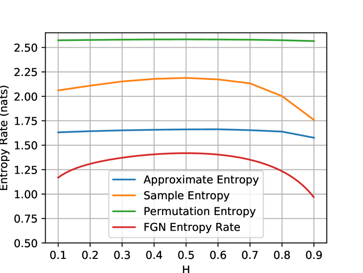
Figure 2: Approximate, sample and permutation entropy estimates for FGN. Note the wide discrepencies.

Figures 3(b) and 3(a) show the entropy rate estimates for the Sample and Approximate Entropy for both Fractional Gaussian Noise and ARFIMA(0,d,0) for two different parameters $m=2,3$ and $r=0.2$ as recommended in Delgado-Bonal and Marshak [10].

Sample Entropy approximates the the shape of the real entropy rate functions but provides large overestimates. This reinforces the use of Sample Entropy as a relative measure of complexity of a time series, as long as it is not used generally for the estimation of differential entropy rate.

Approximate Entropy, however, fails to even approximate trend or range of values. Interestingly, this technique is also quite sensitive to changes in the value of $m$.

Figure 3(c) shows the Permutation Entropy of order $n=3$. These results are indicate that permutation entropy is not a good choice for strongly correlated process as all the behaviour exists on a very small scale, with small differences across the range of $H$. The maximum Permutation Entropy for $n=3$, is $H(\pi)=\log_{2}(3!)\approxeq 2.585$, and all of the estimates are within 0.2 of the maximum value. Similar to Approximate and Sample entropy, from Figure 2 although the trend looks promising on a small scale, once we compare the behaviour to the actual entropy rate, it is a poor estimator of the actual entropy rate.

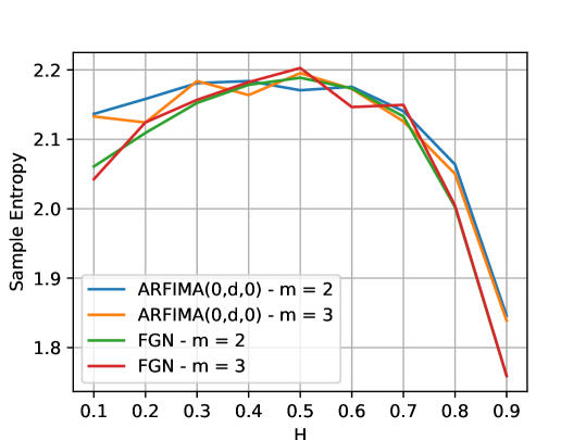
(a) Sample Entropy ($r=0.2$) shows the rough trend of the LRD processes, however it overestimates the differential entropy by a large amount.

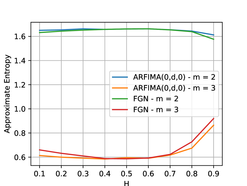
(b) Approximate Entropy ($r=0.2$) fails to even approximate trend or range of values. Interestingly, this technique is also quite sensitive to changes in the value of $m$.

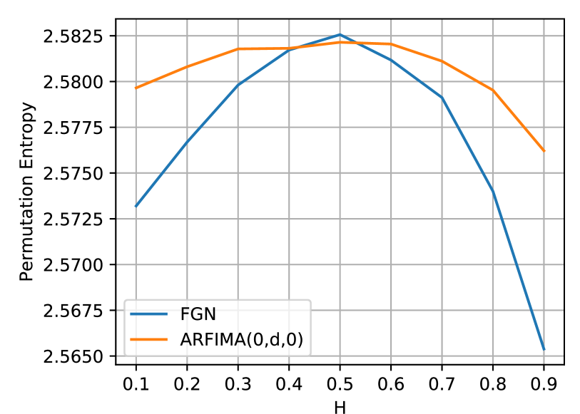
(c) Permutation Entropy (order 3) appears to capture the trend of the entropy rate function, however the scale of the changes is wrong. Noting that the maximum Permutation Entropy is $\log_{2}(3!)\approx 2.585$ the range displayed is very small.

Figure 3: Detailed entropy-rate estimates of FGN and ARFIMA(0,d,0) with process variance $\sigma^{2}=1$.

Naively, these estimates can be improved by extending the lengths of the windows being used, however, for LRD processes large windows would be required. Unfortunately the computational complexity of the approaches (see Table I) grows with increased window sizes and we see stability problems at least with Approximate Entropy, so there does not appear to be a suitable trade-off between computational cost and accuracy.

Estimates derived from Specific Entropy are shown in Figures 4(a) and 4(b), with $p=10$. Specific entropy provides good agreement with the entropy rate for LRD FGN and ARFIMA(0,d,0), i.e.,$H>\frac{1}{2}$, with greater divergence occuring in the CSRD parameter range for small $H$ values. However, note that the computational cost for these estimates is very high.

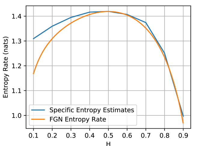
(a) FGN.

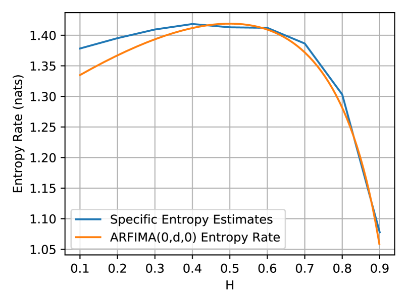
(b) ARFIMA(0,d,0).

Figure 4: Specific Entropy ($p=10$). These estimates are very good over the range of $H$, however the estimates start to diverge for smaller values of $H$.

VI Shannon and Differential Entropy

In this section, we make a connection between the differential and Shannon entropy rate, which we use as the basis of an estimation technique. We propose an approach where we quantise the continuous valued process into a discrete valued process, for a defined quantisation window size, $\Delta$, then apply estimators from the discrete valued domain, and then translate back to differential entropy.

Given the definitions of Shannon and Differential entropy, Definitions II.1 and II.4 respectively, we utilise a connection that exists between these quantities for a quantised version of continuous data, which is given by the following theorem [6, pg. 248].

Theorem VI.1 (Theorem 8.3.1 Cover and Thomas [6]).

If the density $f(x)$ of a random variable $X$ is Riemann integrable, then

$$H(X^{\Delta})+\log(\Delta)\rightarrow h(X),\text{ as }\Delta\rightarrow 0.$$

Therefore the entropy of an n-bit quantisation of a continuous random variable $X$ is approximately $h(X)+n$, when using $\log_{2}$ in the expression above.

Hence, if we quantise and apply Shannon entropy estimators we may be able to make a useful estimation of differential entropy, particularly with finer quantisations and more data. We extend this relationship to the case of Shannon entropy rate and differential entropy rate, which we clarify in the following theorem.

Theorem VI.2.

If the joint density function, $f(x_{1},...,x_{n})$, of the stochastic process, $\raisebox{0.0pt}{$\chi$}=\{X_{m}\}_{m\in\mathbb{N}}$ is Riemann integrable $\forall n\in\mathbb{N}$, then

$$H(\raisebox{0.0pt}{$\chi$}^{\Delta})+\log(\Delta)\rightarrow h(f)=h(\raisebox{0.0pt}{$\chi$}),\text{ as }\Delta\rightarrow 0.$$

Therefore, the entropy rate of an n-bit quantisation of a continuous-valued, discrete-time stochastic process, $\chi$ is approximately $h(\raisebox{0.0pt}{$\chi$})+n$, when using $\log_{2}$ in the expression above.

Proof.

For all finite $n\in\mathbb{N}$, the joint density of the finite collection of random variables is given by $f(x_{1},...,x_{n})$. For notational convenience we use

$$f(x_{1},...,x_{n}) =f(\mathbf{x}),$$

$$f(x_{i^{1}},...,x_{i^{n}}) =f(\mathbf{x_{i}}),$$

$$Pr(x_{1},...,x_{n}) =Pr(\mathbf{x}),$$

$$Pr(x_{i^{1}},...,x_{i^{n}}) =Pr(\mathbf{x_{i}}),$$

$$\text{and }dx_{1}\ldots dx_{n} =d\mathbf{x}.$$

We partition the range of each random variable, $X$ of $\chi$ into bins of length $\Delta$. Now, by the mean value theorem, for any probability density function $f(x)$ there exists $x^{(i^{j})}\in[i^{j}\Delta,(i^{j}+1)\Delta)$ in each bin, such that

$$f(x_{i^{j}})\Delta=\int_{i^{j}\Delta}^{(i^{j}+1)\Delta}f(x)dx.$$

Extending the result to the joint density $\exists\text{ }x_{i^{1}},...,x_{i^{n}}$, such that

$$f(x_{i^{1}},...,x_{i^{n}})\Delta^{n}=\int_{i^{1}\Delta}^{(i^{1}+1)\Delta}...\int_{i^{n}\Delta}^{(i^{n}+1)\Delta}f(\mathbf{x})d\mathbf{x}.$$

We define the quantised stochastic process, $\raisebox{0.0pt}{$\chi$}^{\Delta}=\{X_{m}^{\Delta}\}_{m\in\mathbb{N}}$, by defining each of the quantised random variables $\forall i^{j}$ as,

$$X_{i^{j}}^{\Delta}=x_{i^{j}},\text{ if }i^{j}\Delta\leq X_{i^{j}}<(i^{j}+1)\Delta.$$

Then the probability that $\left(X_{1}^{\Delta},...,X_{n}^{\Delta}\right)=\left(x_{i^{1}},...,x_{i^{n}}\right)$, is given by,

$$Pr(\mathbf{x_{i}}) =\int_{i^{1}\Delta}^{(i^{1}+1)\Delta}...\int_{i^{n}\Delta}^{(i^{n}+1)\Delta}f(\mathbf{x})d\mathbf{x},$$

$$=f(\mathbf{x_{i}})\Delta^{n}.$$

Hence, we consider the joint Shannon entropy of the quantised random variable,

$$H(X_{1}^{\Delta},...,X_{n}^{\Delta}) =-\sum_{i_{1}=-\infty}^{\infty}\ldots\sum_{i_{n}=-\infty}^{\infty}Pr(\mathbf{x_{i}})\log(Pr(\mathbf{x_{i}})),$$

$$=-\sum_{i_{1}=-\infty}^{\infty}\ldots\sum_{i_{n}=-\infty}^{\infty}f(\mathbf{x_{i}})\Delta^{n}\log(f(\mathbf{x_{i}})\Delta^{n}),$$

$$=-\sum_{i_{1}=-\infty}^{\infty}\ldots\sum_{i_{n}=-\infty}^{\infty}f(\mathbf{x_{i}})\Delta^{n}\log(f(\mathbf{x_{i}}))$$

$$\qquad-\sum_{i_{1}=-\infty}^{\infty}\ldots\sum_{i_{n}=-\infty}^{\infty}f(\mathbf{x_{i}})\Delta^{n}\log(\Delta^{n}).$$

As the joint density, $H(X_{1}^{\Delta},...,X_{n}^{\Delta})$, is Riemann integrable $\forall n\in\mathbb{N}$, this implies that as $\Delta\rightarrow 0$,

$$-\sum_{i_{1}=-\infty}^{\infty}\ldots\sum_{i_{n}=-\infty}^{\infty} f(\mathbf{x_{i}})\Delta^{n}\log(f(\mathbf{x_{i}}))$$

$$=-\int_{-\infty}^{\infty}\ldots\int_{-\infty}^{\infty}f(\mathbf{x})\log f(\mathbf{x})d\mathbf{x},$$

$$=h(X_{1},\ldots,X_{n}).$$

Since $f(\mathbf{x_{i}})$ is a joint density over $\mathbb{R}^{n}$, this implies that,

$$\sum_{i_{1}=-\infty}^{\infty}\ldots\sum_{i_{n}=-\infty}^{\infty}f(\mathbf{x_{i}})\Delta^{n} =\int_{-\infty}^{\infty}\ldots\int_{-\infty}^{\infty}f(\mathbf{x_{i}})d\mathbf{x}$$

$$=1.$$

Therefore, we get as $\Delta\rightarrow 0$,

$$H(X_{1}^{\Delta},\ldots,X_{n}^{\Delta})+n\log(\Delta)\rightarrow h(X_{1},\ldots,X_{n}).$$

Now we consider the limit of the quantised joint differential entropy, as the length of the joint entropy tends to infinity,

$$\lim\limits_{n\rightarrow\infty}\frac{1}{n}\left(H(X_{1}^{\Delta},\ldots,X_{n}^{\Delta})+n\log(\Delta)\right) \rightarrow$$

$$\lim\limits_{n\rightarrow\infty}\frac{1}{n} \left(h(X_{1},\ldots,X_{n})\right),$$

and substituting the definitions of Shannon and differential entropy rate respectively, we get

$$\implies H(\raisebox{0.0pt}{$\chi$}^{\Delta})+\log(\Delta) \rightarrow h(\raisebox{0.0pt}{$\chi$}).$$

∎

There will, however, be an error which is due to the difference between the real differential entropy rate, and the approximation of the integral at the quantisation size, $\Delta$.

Another thing to note is that as the quantisation window gets finer, i.e., as $\Delta$ gets smaller, the term in the estimator, $\log(\Delta)\rightarrow-\infty$. There is a potential concern that this disparity between the correction term and the actual estimate could lead to numerical errors. Thus, smaller quantisations aren’t necessarily better for practical estimation.

VII NPD-Entropy Estimator

Theorem VI.2 gives us a way to convert an estimator of entropy rate for discrete-valued, discrete-time stochastic processes into an estimator for a continuous-valued process. We call this strategy NPD-Entropy estimation and explore its properties in this section. In particular we develop links from the properties of the Shannon entropy rate estimator that is selected to the corresponding NPD-estimator.

Definition VII.1 (NPD-Entropy).

The NPD-Entropy estimator of the differential entropy rate, $h(\raisebox{0.0pt}{$\chi$})$, of a continuous-valued, discrete time stochastic process, $\raisebox{0.0pt}{$\chi$}=\{X_{i}\}_{i\in\mathbb{N}}$, using a Shannon entropy rate estimator, $H(\raisebox{0.0pt}{$\chi$}^{\Delta})$, of the corresponding quantised discrete-time, discrete-valued stochastic process $\raisebox{0.0pt}{$\chi$}^{\Delta}=\{X_{i}^{\Delta}\}_{i\in\mathbb{N}}$ with window size, $\Delta$, is defined as

$$\hat{h}_{NPD}(\raisebox{0.0pt}{$\chi$})=\hat{H}(\raisebox{0.0pt}{$\chi$}^{\Delta})+\log\Delta.$$

We analyse some properties of NPD-Entropy and start by considering the consistency of the estimation technique.

Theorem VII.1.

NPD-Entropy, $\hat{h}_{NPD}$, is a consistent estimator as $\Delta\rightarrow 0$, if and only if the associated Shannon entropy rate estimator, $\hat{H}$, is consistent, i.e., as $\Delta\rightarrow 0$ the following two are equivalent:

$$\lim\limits_{n\rightarrow\infty}\hat{H}(\raisebox{0.0pt}{$\chi$}^{\Delta}_{n}) \rightarrow H(\raisebox{0.0pt}{$\chi$}^{\Delta})\,a.s.,$$

$$\lim\limits_{n\rightarrow\infty}\hat{h}_{NPD}(\raisebox{0.0pt}{$\chi$}_{n}) \rightarrow h(\raisebox{0.0pt}{$\chi$})\,a.s.,$$

where $n$ denotes the length of the data sequence to which the estimator is applied.

Proof.

By definition

$$\lim\limits_{n\rightarrow\infty}\hat{h}_{NPD}(\raisebox{0.0pt}{$\chi$}_{n}) = \lim\limits_{n\rightarrow\infty}\hat{H}(\raisebox{0.0pt}{$\chi$}^{\Delta}_{n})+\log\Delta$$

$$= \log\Delta+H(\raisebox{0.0pt}{$\chi$}^{\Delta}).$$

Hence, by Theorem VI.2, the limiting properties of the two are linked. ∎

Remark.

This is a very general result, that only relies on the existence of a consistent estimator for Shannon entropy rate. The argument is agnostic to the mode of convergence used, and the strength of the convergence depends on which mode of convergence is used for the consistency of the Shannon entropy rate estimator.

We explore more general results for the variance, mean squared error, and then apply these to efficiency, as efficiency is applied to unbiased estimators of the entropy rate.

Theorem VII.2.

The NPD-Entropy, $\hat{h}_{NPD}$, constructed from an estimator of the Shannon entropy rate, $\hat{H}$ has the following properties

1. $\mbox{Bias}_{h}[\hat{h}_{NPD}(\raisebox{0.0pt}{$\chi$}_{n})]=\mbox{Bias}_{H}[\hat{H}(\raisebox{0.0pt}{$\chi$}^{\Delta}_{n})]$,

2. $\mbox{Var}(\hat{h}_{NPD}(\raisebox{0.0pt}{$\chi$}_{n}))=\mbox{Var}(\hat{H}(\raisebox{0.0pt}{$\chi$}^{\Delta}_{n}))$,

3. $\mbox{MSE}(\hat{h}_{NPD}(\raisebox{0.0pt}{$\chi$}_{n}))=\mbox{MSE}(\hat{H}(\raisebox{0.0pt}{$\chi$}^{\Delta}_{n}))$,

as $\Delta\rightarrow 0$.

Proof.

From the definition of bias [29, pg. 126], we have

$$\mbox{Bias}_{H}[\hat{H}] =E[\hat{H}]-H,$$

$$=E[(\hat{h}_{NPD}-\log\Delta)]-(h-\log\Delta),\text{ as }\Delta\rightarrow 0$$

$$=E[\hat{h}_{NPD}]-h,$$

$$=\mbox{Bias}_{h}[\hat{h}_{NPD}].$$

The result for the mean squared error of the estimator follows by an identical argument, substituting, $\hat{h}_{NPD}-\log\Delta$ and $h-\log\Delta$ for $\hat{H}$ and $H$ respectively as $\Delta\rightarrow 0$, therefore we omit the argument.
We consider another characterisation of the mean squared error, known as the bias-variance decomposition [14, pg. 24],

$$\mbox{MSE}[\hat{H}] =\mbox{Bias}_{H}[\hat{H}]^{2}+\mbox{Var}(\hat{H}),$$

and placing in terms of the variance and substituting the bias and mean square error equivalences as $\Delta\rightarrow 0$, we get

$$\mbox{Var}(\hat{H}) =\mbox{Bias}_{H}[\hat{H}]^{2}-\mbox{MSE}[\hat{H}],$$

$$=\mbox{Bias}_{h}[\hat{h}_{NPD}]^{2}-\mbox{MSE}[\hat{h}_{NPD}],\text{ as }\Delta\rightarrow 0,$$

$$=\mbox{Var}(\hat{h}_{NPD}).$$

∎

We investigate the asymptotic normality of the Shannon entropy rate estimator, That is, the asymptotic distribution of the estimator being a normally distributed random variable.

Theorem VII.3.

NPD-Entropy, $h$, is asymptotically normal as $\Delta\rightarrow 0$ if the associated Shannon entropy rate estimator, $H$, is consistent and asymptotically normal.

Proof.

Given a $\sigma^{2}\in\mathbb{R^{+}}$, for $n\rightarrow\infty$ with an asymptotically normal estimator we have,

$$\sqrt{n}\left(\hat{H}(\raisebox{0.0pt}{$\chi$}^{\Delta}_{n})-H\right) \rightarrow\mathcal{N}(0,\sigma^{2}).$$

Substituting the expression for the differential entropy rate,we get

$$\sqrt{n}\left((\hat{h}_{NPD}(\raisebox{0.0pt}{$\chi$}_{n})-\log\Delta)-(h-\log\Delta)\right) \rightarrow$$

$$\mathcal{N}(0,\sigma^{2}), \text{ as }\Delta\rightarrow 0,$$

and we conclude

$$\sqrt{n}\left(\hat{h}_{NPD}(\raisebox{0.0pt}{$\chi$}_{n})-h\right) \rightarrow\mathcal{N}(0,\sigma^{2}).$$

∎

The next property we examine is the efficiency, which is,

$$e(T)=\frac{I(\theta)^{-1}}{Var(T)},$$

for an unbiased estimator, $T$, of a parameter, $\theta$, where $I(\theta)=E\left[\left(\frac{\partial}{\partial\theta}\log f(T;\theta)\right)^{2}\mid\theta\right]$ is the Fisher information [7, pg. 481]. Efficiency of an estimator measures the variance of the estimator with respect to the lowest possible variance, the Cramer-Rao bound [7, pg. 480], which is when $e(T)=1$.

Theorem VII.4.

The efficiency of NPD-Entropy, $e(\hat{h}_{NPD}(\raisebox{0.0pt}{$\chi$}_{n}))$ is equal to the efficiency of the Shannon entropy rate estimator, $e(\hat{H}(\raisebox{0.0pt}{$\chi$}^{\Delta}_{n}))$ for a Riemann integrable probability density function for the process, $\raisebox{0.0pt}{$\chi$}=\{X_{i}\}_{i\in\mathbb{N}}$.

Proof.

We consider the Fisher information of the quantised process,

$$I_{\raisebox{0.0pt}{$\chi$}^{\Delta}}(H) =\sum_{i}\left(\frac{d}{dH}\log p_{i}\right)^{2}p_{i},$$

$$=\sum_{i}\left(\frac{d}{dH}\log(f(x_{i})\Delta)\right)^{2}f(x_{i})\Delta.$$

Where $p_{i}=\int_{i^{j}\Delta}^{(i^{j}+1)\Delta}f(x)dx=f(x_{i^{j}})\Delta$, since the density is Riemann integrable. Therefore the Fisher information is

$$I_{\raisebox{0.0pt}{$\chi$}^{\Delta}}(H) =\sum_{i}\left(\frac{d}{dH}\log f(x_{i})+\log\Delta\right)^{2}f(x_{i})\Delta,$$

$$=\sum_{i}\left(\frac{d}{dH}\log f(x_{i})\right)^{2}f(x_{i})\Delta,$$

since $\log\Delta$ is constant with respect to $H$. Then

$$I_{\raisebox{0.0pt}{$\chi$}^{\Delta}}(H) =\int\left(\frac{d}{dh}\log f(x)\right)^{2}f(x)dx,\text{ as }\Delta\rightarrow 0,$$

$$=I_{\raisebox{0.0pt}{$\chi$}}(h).$$

Where $\frac{dH}{df}=\frac{d(h-\log\Delta)}{df}=\frac{dh}{df}$, for a given function $f$, as $\Delta\rightarrow 0$.
Now we, consider the efficiency of the differential entropy rate estimator,

$$e(\hat{h}_{NPD}) =\frac{\frac{1}{I(h)}}{\mbox{Var}(\hat{h}_{NPD})},$$

$$=\frac{\frac{1}{I(H)}}{Var(\hat{H})},\text{ from Theorem\leavevmode\nobreak\ \ref{bias_var_mse}},$$

$$=e(\hat{H})$$

∎

Another property of interest is the convergence rate of an estimator, as we often want to understand how long it would take to be within a certain distance from the real value, to understand how much data is required for estimation.

Theorem VII.5.

The convergence rate of NPD-Entropy, $\hat{h}_{NPD}(\raisebox{0.0pt}{$\chi$}_{n})$ is equal to the convergence rate of the Shannon entropy rate estimator, $\hat{H}(\raisebox{0.0pt}{$\chi$}^{\Delta}_{n})$ as $\Delta\rightarrow 0$.

Proof.

For the convergence rate, $C(n)$, of a Shannon entropy rate estimator, we have $\forall n\in\mathbb{N}$,

$$Pr(|\hat{H}(\raisebox{0.0pt}{$\chi$}^{\Delta}_{n})-H|>\epsilon) \leq C(n).$$

Then making the substitution of the differential entropy rate estimator, and cancelling out the $\log\Delta$ terms, we get

$$Pr(|\hat{h}_{NPD}(\raisebox{0.0pt}{$\chi$}_{n})-h|>\epsilon) \leq C(n).$$

∎

VII-A Implementation and Initial Results

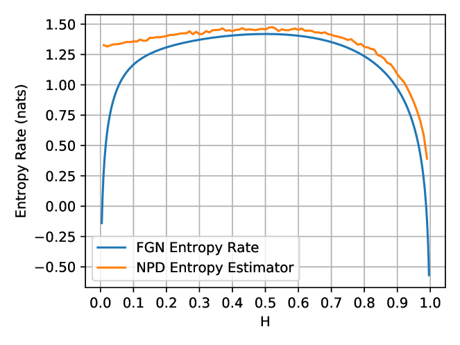
(a) Comparison for Fractional Gaussian Noise. The estimates have a small bias, but get poorer as $H\rightarrow 0$ and the entropy rate function asymptotically tends to $-\infty$.

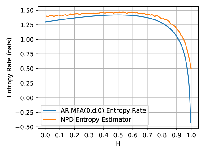
(b) Comparison for ARFIMA(0,d,0). Note the close correspondence, with a small bias.

Figure 5: NPD Entropy with $\Delta=1$ compared to actual entropy rate of FGN and ARFIMA(0,d,0). With $\Delta=1$, the Shannon entropy rate estimator is directly used as the NPD-Entropy estimate.

To test this concept, we have implemented an estimator using the discrete-valued estimator described in Section III. The conditions in Kontoyiannis and Suhov [20] were used to ensure that we produce a consistent Shannon entropy rate estimator.

The estimator was implemented in Python using the NumPy library [17]. We parallelised the implementation of NPD Entropy to increase the performance of the estimation technique since we can calculate the length of each prefix sequence, $L^{n}(x)$, independently. This has been implemented using the Python library Numba [23], which is able to parallelise the loop to calculating the prefixes, $L(x)$. The algorithm can be run online, for quick estimation of entropy rates of streaming data.

The estimators were tested on data generated by FGN and ARFIMA(0,d,0) processes. We generated 50 test samples of 2000 data points for each process. The estimates for each process were then averaged, to show the mean estimate at each value of $H$.

From observing both Figure 5(a) and Figure 5(b), utilising a quantised interval size of 1 (i.e. $\Delta=1$), we see overall good agreement, except in the region $H\rightarrow 0$ for FGN. In all cases the NPD-Entropy estimator was better at picking up the underlying trends of the entropy rate functions than the relative measures tested in Section V, but specific entropy produced closer estimates of the differential entropy rate at a large cost in computation time.

The limit theorems and the results on the inherited properties, from Section VII, of the estimator hold as $\Delta\rightarrow 0$, which for practical purposes we are unable to achieve. However, this leaves us with trying to understand the possible errors that have been introduced. Potential sources of estimation error are from the difference of the Riemann sums and the value of the integral, i.e., as $\sum f(x)\rightarrow\int f(x)$. As the quantisation window decreases, as $\Delta\rightarrow 0$, small differences from the true value and estimated values can be enlarged by the term $\log\Delta$. To test the deviation from true value, we produced estimates for a range of different quantisation window sizes, $\frac{1}{3},\frac{1}{2},1,2,3$, for the Hurst parameter range, $[0,1]$. Given that we have standardised all of the process variances to be $\sigma^{2}=1$, the window size is in direct proportion with the variance. This means that small fluctuations of the process will stay within same bin, and therefore the measured uncertainty will come from larger shifts. In general we would tailor the window size to the variance, since we want to balance the number of bins and the expected size of movements between random variables of the process.

The results for FGN are shown in Figure 6(a). The most accurate of these across the whole range is at $\Delta=1$, which is surprising as we should be more accurate as the quantisation size decreases. However, we are balancing a few different sources of error and in this case the best result is to quantise at a window size of 1. However, as the Hurst parameter tends to 1, the finer quantisations become more accurate estimators. As the correlations become stronger the variation in the process will be more subtle, hence the smaller quantisation windows are required to estimate the uncertainty.

The results are similar for ARFIMA(0,d,0) processes, with the closest estimator, across the entire parameter range, being when the quantisation window was of size, $\Delta=1$. The estimators got worse as $\Delta$ got further from 1, i.e. the next closest were $\Delta=\frac{1}{2}$ and $2$. The finer quantisations, $\Delta=\frac{1}{2},\frac{1}{3}$ became more accurate as $H$ increased.

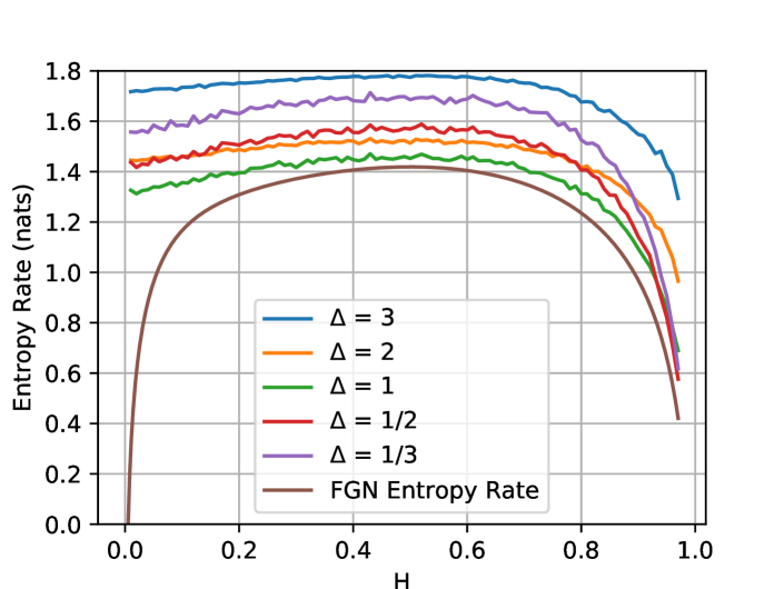
(a) Comparison of the quantised estimates and true values of differential entropy rate of FGN. The window size of one has the best estimates, however as the Hurst parameter tends to one the finer quantisations, i.e., $\frac{1}{3}$ and $\frac{1}{2}$, approximate the asymptotic decrease better.

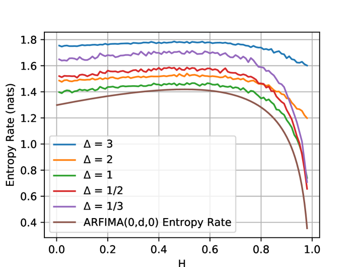
(b) Comparison of the quantised estimates and true values of differential entropy rate of ARFIMA(0,d,0). Similar to FGN, the window size of $1$ provides the best estimates over the range of Hurst parameter values, however we also see that the finer quantisations become more accurate as $H$ increases towards $1$.

Figure 6: NPD Entropy with $\Delta=\frac{1}{3},\frac{1}{2},1,2,3$ compared to actual entropy rate of FGN and ARFIMA(0,d,0)

VII-B Robustness of estimator to non-stationarity

A common assumption that is made to enable analysis of stochastic processes and for data generating processes, is stationarity, meaning that the probability distribution is time invariant over the stochastic processes.

Definition VII.2.

A stochastic process, $\raisebox{0.0pt}{$\chi$}=\{X_{i}\}_{i\in\mathbb{N}}$, with a cumulative distribution function for its joint distribution at times, $t_{1}+\tau,\ldots,t_{n}+\tau$, of, $F_{X}(t_{1}+\tau,\ldots,t_{n}+\tau)$. We say that the process is stationary if $F_{X}(t_{1}+\tau,\ldots,t_{n}+\tau)=F_{X}(t_{1},\ldots,t_{n}),\forall\tau>0,t_{1},\ldots,t_{n}\in\mathbb{R},\forall n\in\mathbb{N}$.

Many real world processes are not really stationary, hence we want to analyse how robust the quantised estimation technique is to non-stationarity. In the previous section we have shown that the estimator has good performance in the cases of strongly correlated processes. However, we would like to test the performance against processes that have a convergent entropy rate, but have moment statistics that vary with time.

The initial test for a departure from stationarity is a mean-shifting process. We define this as $X_{n}=\mu_{n}+\epsilon_{n}$, where $\epsilon_{n}\sim\mathcal{N}(0,1)$ and independent and where $\mu_{n}$ alternates periodically between 0 and 1 every 100 samples.The mean shifts are predictable so the entropy rate is

$$h\left(\mu_{n}+\epsilon_{n}\right) =h\left(\epsilon_{n}\right)=\frac{1}{2}\log(2\pi e)\approx 1.419.$$

We test this process with 50 realisations of 2000 data points. The mean and variance of the estimates are shown in Table II. NPD-Entropy, with a choice of parameter $\Delta=1$, made an estimate of the entropy rate of 1.554, which overestimates the true value by a small amount, similar to specific entropy. Sample and permutation entropy both provided large overestimates of the true value, with permutation entropy having an extremely low variance, close to its maximum value, $\log(3!)\approx 2.585$. Approximate entropy was a large underestimate, similar to the behaviour with $m=3$ for both the ARFIMA(0,d,0) and FGN estimates.

The second test for robustness to a departure from non-stationarity is to consider a simple model that has a stationary mean, but varying second order statistics, a Gaussian Random Walk, $\{Z_{n}\}_{n\in\mathbb{N}}$. Each step, $X_{i}\sim\mathcal{N}(0,1)$ is independent and we consider the sum of the steps $Z_{n}=\sum_{i=1}^{n}X_{i}$. The entropy rate can be derived by considering the limiting conditional entropy to give $h(Z_{n})=h(X_{n})\approx 1.419$. However, the process has non-stationary second moment $\mbox{Var}(Z_{n})=n$.

These initial results suggest that specific entropy is relatively robust, but its alternatives are not. However NPD-Entropy is somewhat robust to mean shifts, if not to changes in variance. The variance in this case is constantly growing in proportional to the number of random samples of the process, as opposed to the previous process which had non-stationarity in its mean, but a constant variance of the normally distributed noise. This may explain the difficulty of capturing the true value in this case, as all of the bins are likely to have small numbers of observations, unless large amounts of data points are observed. Therefore, we have to be careful in how processes depart from stationarity, to understand how closely we can estimate the true entropy rate.

	Mean Shift		Gaussian Walk
Estimation Technique	Mean	Variance	Mean	Variance
Approximate Entropy	$0.482$	$0.0008$	$0.099$	$0.0007$
Sample Entropy	$2.263$	$0.015$	$2.336$	$0.205$
Permutation Entropy	$2.582$	$0.000005$	$2.497$	$0.0002$
Specific Entropy	$1.478$	$0.0005$	$1.523$	$0.0007$
NPD-Entropy	$1.554$	$0.002$	$2.385$	$0.083$

Table II: Differential entropy rate estimates applied to two non-stationary processes: a Gaussian i.i.d. mean shift and a Gaussian walk with entropy rates 1.419. Each process was simulated 50 times. The relative measures, the sample entropy and permutation entropy both provide large overestimates of the true entropy, and approximate entropy provides large underestimates. NPD-entropy behaves only slightly worse than specific entropy on the mean-shift process, but somewhat worse on the Gaussian walk. Estimator variances are included to inform about the relative size of the errors.

VII-C Complexity Analysis of Estimation Techniques

The worst-case asymptotic time complexities of the estimators tested here are shown in Table I. Approximate entropy has two loops which run to calculate the quantity, first to calculate every $C_{i}^{m}(r)$, the number of strings that exceed a threshold, by fixing one of the substrings, then a second loop over all of the $C_{i}^{m}(r)$’s, i.e., for a pairwise comparison of all substrings. Hence, the time complexity is approximately $O(N^{2})$, where $N$ is the length of data. Sample entropy requires two separate loops, which run over the substrings of order $m$ and $m+1$ all calculating the number of pairs that exceed a threshold, i.e., two loops of order $N^{2}$, which also results in a pairwise comparison and hence the time complexity is approximately $O(N^{2})$. Permutation entropy takes the relative frequency of each possible permutation, of order $n$, of which there exist $n!$ permutations. This is performed across the entire data set, and hence the worst-case time complexity for permutation entropy is $O(n!N)$, and hence is extremely sensitive to the choice of order $n$. With appropriate choices of order this can be used as an quick measure of complexity of time series, however it does grow extremely quickly with the order of permutation and hence there is a trade off here between how much data is available with what order can be selected for this technique.

Specific entropy’s complexity depends on the choice of kernel density estimator. We used their implementation in R which used the package np for non-parametric kernel density estimation [8]. The technique calculates the bandwidth parameters and then calculates the product and univariate kernel estimates for windows of length $p$. Hence, to make an estimate we do $N$ kernel density evaluations, and therefore $Np$ for the calculation of the estimate of the joint density per window, and hence with a loop over all of the windows we get an approximate complexity of $O(N^{2}p)$. Although this does not appear substantially worse that the other estimators, the actual amount of computation is dramatically larger.

NPD Entropy has two steps: (i) quantisation and (ii) a Shannon entropy rate estimator, which in most cases will dominate the performance. In our case we use the Grassberger estimate, which utilises string-matching based on Lempel-Ziv algorithm [38], which has a complexity of $O(N\log N)$, using the algorithm of Grassberger [16].

Complexity estimates are useful to understand scaling properties, but the actual computation times for finite data can be dominated by non-asymptotic terms, and so we test performance directly using 1000 estimates of $N=1000$ data points. Tests were performed on a 2.4GHz Intel Core i5 processor with 8GB of RAM, running MacOS 10.14.6. The results are shown in Table I. Approximate entropy was much slower than sample entropy, with permutation entropy being the fastest by far. However NPD-Entropy is faster than all but permutation entropy and runs extremely quickly compared to specific entropy. The specific entropy was considerably slower than all the measures with the 1000 estimates being in the order of 6 days.

Given the time complexity, we suggest using NPD-Entropy as an efficient way of classifying complexity of a system. NPD-Entropy provides a more accurate and robust measurement with comparable or better computation times than most alternatives. Specific entropy is still superior for accurate measures, but computationally prohibitive except where accuracy is the only criteria.

VIII Conclusion

We have defined a new technique for the non-parametric estimation of the differential entropy rate. We have made an explicit link between the differential entropy rate and the Shannon entropy rate of the associated quantised process. This forms the basis of the estimation technique, NPD Entropy, by quantising the continuous data and utilising the existing theory of Shannon entropy rate estimation. We have shown that this estimation technique inherits statistical properties from the Shannon entropy rate estimator and performs better than other differential entropy rate estimators in the presence of strongly correlated data.

In addition, we have investigated the robustness to non-stationarity of the estimation technique, and provided over-estimates of the entropy. More research is required to analyse the robustness to non-stationarity and understand if the influence is similar to the Shannon entropy rate case. Finally, we have demonstrated the utility of NPD Entropy and shown that it can be run quickly and efficiently to make decent estimates if used in an online mode.

References

- [1] R. Alcaraz and J. J. Rieta. A review on sample entropy applications for the non-invasive analysis of atrial fibrillation electrocardiograms. Biomedical Signal Processing and Control, 5(1):1–14, 2010.
- [2] C. Bandt and B. Pompe. Permutation entropy: a natural complexity measure for time series. Physical review letters, 88(17):174102, 2002.
- [3] C. Bandt and F. Shiha. Order patterns in time series. Journal of Time Series Analysis, 28(5):646–665, 2007.
- [4] J. Beran. Statistics for Long-Memory Processes. Chapman & Hall/CRC Monographs on Statistics & Applied Probability. Taylor & Francis, 1994.
- [5] X. Chen, I. C. Solomon, and K. H. Chon. Comparison of the use of approximate entropy and sample entropy: applications to neural respiratory signal. In 2005 IEEE Engineering in Medicine and Biology 27th Annual Conference, pages 4212–4215. IEEE, 2006.
- [6] T. M. Cover and J. A. Thomas. Elements of Information Theory (Wiley Series in Telecommunications and Signal Processing). Wiley-Interscience, USA, 2006.
- [7] H. Cramér. Mathematical methods of statistics, volume 43. Princeton university press, 1999.
- [8] D. Darmon. Specific differential entropy rate estimation for continuous-valued time series. Entropy, 18(5):190, 2016.
- [9] D. Darmon. Information-theoretic model selection for optimal prediction of stochastic dynamical systems from data. Physical Review E, 97(3):032206, 2018.
- [10] A. Delgado-Bonal and A. Marshak. Approximate entropy and sample entropy: A comprehensive tutorial. Entropy, 21:541, 05 2019.
- [11] R. Durrett. Probability: Theory and Examples. Cambridge University Press, New York, NY, USA, 4th edition, 2010.
- [12] J.-P. Eckmann and D. Ruelle. Ergodic theory of chaos and strange attractors. In The theory of chaotic attractors, pages 273–312. Springer, 1985.
- [13] A. Feutrill and M. Roughan. Differential entropy rate characterisations of long range dependent processes, 2021. arXiv preprint http://arxiv.org/abs/2102.05306arXiv:2102.05306.
- [14] J. Friedman, T. Hastie, and R. Tibshirani. The elements of statistical learning, volume 1. Springer series in statistics New York, 2001.
- [15] A. Gefferth, D. Veitch, I. Maricza, S. Molnár, and I. Ruzsa. The nature of discrete second-order self-similarity. Advances in Applied Probability, pages 395–416, 2003.
- [16] P. Grassberger. Estimating the information content of symbol sequences and efficient codes. IEEE Transactions on Information Theory, 35(3):669–675, 1989.
- [17] C. R. Harris, K. J. Millman, S. J. van der Walt, R. Gommers, P. Virtanen, D. Cournapeau, E. Wieser, J. Taylor, S. Berg, N. J. Smith, R. Kern, M. Picus, S. Hoyer, M. H. van Kerkwijk, M. Brett, A. Haldane, J. F. del R’ıo, M. Wiebe, P. Peterson, P. G’erard-Marchant, K. Sheppard, T. Reddy, W. Weckesser, H. Abbasi, C. Gohlke, and T. E. Oliphant. Array programming with NumPy. Nature, 585(7825):357–362, Sept. 2020.
- [18] J. R. M. Hosking. Fractional differencing. Biometrika, 68(1):165–176, 04 1981.
- [19] H. E. Hurst. Long-term storage capacity of reservoirs. Trans. Amer. Soc. Civil Eng., 116:770–799, 1951.
- [20] I. Kontoyiannis, P. H. Algoet, Y. M. Suhov, and A. J. Wyner. Nonparametric entropy estimation for stationary processes and random fields, with applications to english text. IEEE Transactions on Information Theory, 44(3):1319–1327, 1998.
- [21] I. Kontoyiannis and I. Soukhov. Prefixes and the entropy rate for long-range sources. In Proceedings - 1994 IEEE International Symposium on Information Theory, ISIT 1994, Dec. 1994. 1994 IEEE International Symposium on Information Theory, ISIT 1994 ; Conference date: 27-06-1994 Through 01-07-1994.
- [22] D. E. Lake, J. S. Richman, M. P. Griffin, and J. R. Moorman. Sample entropy analysis of neonatal heart rate variability. American Journal of Physiology-Regulatory, Integrative and Comparative Physiology, 283(3):R789–R797, 2002.
- [23] S. K. Lam, A. Pitrou, and S. Seibert. Numba: A llvm-based python jit compiler. In Proceedings of the Second Workshop on the LLVM Compiler Infrastructure in HPC, LLVM ’15, New York, NY, USA, 2015. Association for Computing Machinery.
- [24] W. E. Leland, M. S. Taqqu, W. Willinger, and D. V. Wilson. On the self-similar nature of ethernet traffic. In Conference Proceedings on Communications Architectures, Protocols and Applications, SIGCOMM ’93, pages 183–193, New York, NY, USA, 1993. ACM.
- [25] B. B. Mandelbrot and J. W. van Ness. Fractional Brownian motions, fractional noises and applications. SIAM Review, 10:422–437, 1968.
- [26] D. S. Ornstein and B. Weiss. Entropy and data compression schemes. IEEE Transactions on Information Theory, 39(1):78–83, 1993.
- [27] S. M. Pincus. Approximate entropy as a measure of system complexity. Proceedings of the National Academy of Sciences, 88(6):2297–2301, 1991.
- [28] A. N. Quas. An entropy estimator for a class of infinite alphabet processes. Theory of Probability & Its Applications, 43(3):496–507, 1999.
- [29] J. A. Rice. Mathematical Statistics and Data Analysis. Belmont, CA: Duxbury Press., third edition, 2006.
- [30] J. S. Richman and J. R. Moorman. Physiological time-series analysis using approximate entropy and sample entropy. American Journal of Physiology-Heart and Circulatory Physiology, 278(6):H2039–H2049, 2000.
- [31] C. E. Shannon. A mathematical theory of communication. Bell Syst. Tech. J., 27(3):379–423, 1948.
- [32] P. C. Shields. Entropy and prefixes. Ann. Probab., 20(1):403–409, 01 1992.
- [33] C. Varotsos and D. Kirk-Davidoff. Long-memory processes in ozone and temperature variations at the region 60° s?60° n. Atmos. Chem. Phys., 6, 09 2006.
- [34] W. Willinger, M. S. Taqqu, R. Sherman, and D. V. Wilson. Self-similarity through high-variability: statistical analysis of ethernet lan traffic at the source level. IEEE/ACM Transactions on Networking, 5(1):71–86, Feb 1997.
- [35] W. Willinger, M. S. Taqqu, and V. Teverovsky. Stock market prices and long-range dependence. Finance and Stochastics, 3(1):1–13, Jan. 1999.
- [36] A. D. Wyner and J. Ziv. Some asymptotic properties of the entropy of a stationary ergodic data source with applications to data compression. IEEE Transactions on Information Theory, 35(6):1250–1258, 1989.
- [37] J. M. Yentes, N. Hunt, K. K. Schmid, J. P. Kaipust, D. McGrath, and N. Stergiou. The appropriate use of approximate entropy and sample entropy with short data sets. Annals of biomedical engineering, 41(2):349–365, 2013.
- [38] J. Ziv and A. Lempel. A universal algorithm for sequential data compression. IEEE Transactions on information theory, 23(3):337–343, 1977.