Extraction of invariant manifolds and application to turbulence with a passive scalar

Abstract

The reduction of dimensionality of physical systems, specially in fluid dynamics, leads in many situations to nonlinear ordinary differential equations which have global invariant manifolds with algebraic expressions containing relevant physical information of the original system. We present a method to identify such manifolds, and we apply it to a reduced model for the Lagrangian evolution of field gradients in homogeneous and isotropic turbulence with a passive scalar.

Fluids, and turbulence in particular, have been a playground for many applications of the theory of dynamical systems. Methods to reduce the number of degrees of freedom of a system have been developed for or applied to fluid dynamics, from truncations using Fourier Lorenz (1963) or empirical modes Holmes et al. (1996), to models that reduce the dimensionality of the Lagrangian evolution of field gradients Li and Meneveau (2005); Chevillard and Meneveau (2006); Meneveau (2011); Johnson and Meneveau (2016); Pereira et al. (2018); Sujovolsky et al. (2019). These latter models often also display global invariant manifolds (GIMs, i.e., manifolds globally preserved under the system evolution) with algebraic expressions, as the Vieillefosse manifold Vieillefosse (1982). Such manifolds play a crucial role in the dynamics, and perturbative methods were developed Guckenheimer and Holmes (1983) to identify them in nonlinear ordinary differential equations (ODEs). Here we present a method to identify GIMs with algebraic expressions, in ODEs as those resulting from reduced models for fluids, and apply it to homogeneous and isotropic turbulence (HIT) with a passive scalar Celani et al. (2000); Watanabe and Gotoh (2007); Buaria et al. (2021). Examples of passive scalars include small temperature fluctuations in a fluid, atmospheric humidity, or chemicals concentration. The concentration also corresponds to the continuous limit of diluted particles, of interest for practical and theoretical reasons Shraiman and Siggia (2000); Falkovich et al. (2001); Donzis and Yeung (2010); Gotoh and Watanabe (2015). However, reduced models for passive scalar gradients have been barely explored. We thus also derive a reduced model for this case. In HIT, similar models, sometimes called restricted Euler models or QR-models, are used to study singularities Vieillefosse (1982) and the origin of non-Gaussian statistics and intermittency Li and Meneveau (2005), among many other applications. Our model in turn can help understand how turbulence affects the passive scalar transport. The results we present are then twofold: A reduced model for field gradients evolution in passive scalar turbulence, and a method to identify GIMs.

We consider the Lagrangian evolution of the gradients of an incompressible velocity field $\bf{u}$ (with $\nabla\cdot{\bf u}=0$) and of a passive scalar $\theta$. The dynamics are given by

$$D_{t}{\bf u}=-{\boldsymbol{\nabla}}p+\nu\nabla^{2}{\bf u}+{\bf f},\,\,\,\,\,\,\,D_{t}\theta=\kappa\nabla^{2}\theta+f_{\theta},$$ (1)

where $D_{t}=\partial_{t}+{\bf u}\cdot{\boldsymbol{\nabla}}$ is the Lagrangian derivative, $p$ the pressure per unit mass density, $\nu$ the kinematic viscosity, $\kappa$ the diffusivity, ${\bf f}$ an external mechanical forcing, and $f_{\theta}$ a scalar source. For $\nu=\kappa$ the equations have one dimensionless parameter that controls the dynamics, the Reynolds number $\mathrm{Re}=u\lambda/\nu$, where $u$ is the r.m.s. flow velocity and $\lambda$ the Taylor microscale, a characteristic scale in turbulence. To compare with the reduced model we performed a direct numerical simulation (DNS) of Eq. (1) in a three-dimensional (3D) periodic cubic domain with spatial resolution of $1024^{3}$ grid points. We used a parallel pseudospectral fully-dealiased method to compute spatial derivatives and nonlinear terms, and a second-order Runge-Kutta scheme for time integration Mininni et al. (2011). A 3D large-scale random forcing ${\bf f}$ was used to sustain the turbulence, and a random scalar source $f_{\theta}$ was applied to inject passive scalar concentration. The viscosity and diffusivity where chosen in such a way that all the relevant flow scales were properly resolved. This resulted in ${\textrm{R}e}\approx 560$, with $k\eta\approx 1.2$, where $k$ is the maximum resolved wavenumber and $\eta$ the Kolmogorov dissipation scale. To study the Lagrangian evolution (i.e., following fluid elements) of velocity and passive scalar gradients, we tracked $10^{6}$ Lagrangian particles for several large-scale turnover times using the methods discussed in Yeung and Pope (1988). Velocity and passive scalar gradients at particles’ positions ${\bf x}$, ${\boldsymbol{\nabla}}{\bf u}({\bf x},t)$ and ${\boldsymbol{\nabla}}\theta({\bf x},t)$, were stored with high time cadence to compute their statistics and time derivatives.

A reduced model for the Lagrangian evolution of field gradients. From Eq. (1) we now derive a closed model for velocity and passive scalar field gradients, based on similar models for velocity gradients in HIT Meneveau (2011). While HIT is sustained out of equilibrium by the external forcing and dissipation, we neglect both and consider the ideal unforced case ($\nu=\kappa={\bf f}=f_{\theta}=0$). We can thus expect the reduced model to give a good approximation to field gradients dynamics only for short times, when the effect of the forcing and of dissipation are small compared with nonlinearities. In spite of this, we will see that the reduced model compares well with results from the DNS. The limit of negligible diffusivity can be interpreted, e.g., as the case of passive scalars in atmospheric turbulence, in which advection dominates. Diffusivity and viscosity (to also consider, e.g., the effect of the Schmidt number) can be later added using the methods described in Meneveau (2011).

When computing spatial derivatives of Eq. (1), we write field gradients using index notation and define $A_{ij}=\partial_{j}u_{i}$ and $\theta_{j}=\partial_{j}\theta$ (for $i$, $j\in\{x,y,z\}$). Then,

$$D_{t}A_{ij}+A_{kj}A_{ik}=-\partial_{ij}p,\,\,\,\,\,\,\,D_{t}\theta_{j}+A_{kj}\theta_{k}=0,$$ (2)

where $\partial_{ij}=\partial_{i}\partial_{j}$. The first equation is the usual Lagrangian evolution equation for the velocity gradient tensor $A_{ij}$, while the second is the Lagrangian evolution equation for passive scalar gradients. Some derivatives of the pressure in Eq. (2) can be removed using the incompressibility condition ${\boldsymbol{\nabla}}\cdot{\bf u}=A_{ii}=0$, which for $D_{t}A_{ii}$ in Eq. (2) implies $A_{ki}A_{ik}=-\partial_{ii}p$. The remaining spatial derivatives of the pressure can be written using the deviatoric part of the pressure Hessian, $H_{ij}=-(\partial_{ij}p-\delta_{ij}\partial_{kk}p/3)$, where $\delta_{ij}$ is the Kronecker delta. The equation for $D_{t}A_{ij}$ can then be written as

$$D_{t}A_{ij}+A_{kj}A_{ik}-\delta_{ij}A_{kl}A_{lk}/3=H_{ij}.$$ (3)

This equation, together with the equation for $D_{t}\theta_{j}$ in Eq. (2), provide a set of equations (albeit not closed) for the evolution of all components of ${\boldsymbol{\nabla}}{\bf u}$ and ${\boldsymbol{\nabla}}\theta$ along the trajectories of fluid elements.

To close this set of equations we use an approximation commonly used in restricted Euler models of HIT Cantwell (1992); Chevillard and Meneveau (2006); Meneveau (2011), and assume that the deviatoric part of the pressure Hessian can be neglected. In other words, we assume that $H_{ij}\approx 0$ in Eq. (3). Attempts have been made to improve this approximation, which otherwise results in a finite time blow up of the reduced model for HIT Wilczek and Meneveau (2014); Carbone et al. (2020); Parashar et al. (2020); such attempts include a multi-scale model that regularizes the singularity and retains the geometrical properties of the QR-model Chevillard et al. (2008). Then we reduce the information in $A_{ij}$ and $\theta_{j}$ to the smallest possible number of scalar quantities resulting in an autonomous system. For the velocity gradients in HIT, two scalar quantities (proportional to the traces of ${\bf A}^{2}$ and ${\bf A}^{3}$ and thus invariant under the group of rotations and reflections, with ${\bf A}$ the velocity gradient tensor) suffice to obtain the QR-model Meneveau (2011). Here, we also want to take into account the scalar gradients in the model. Thus we define

$$Q = -A_{ij}A_{ji}/2,\ \ R=-A_{ij}A_{jk}A_{ki}/3,\ \ S=\sum_{i}\theta_{i}/3,$$

$$T = \sum_{i}\theta_{j}A_{ji}/3,\ \ U=\sum_{i}\theta_{j}A_{jk}A_{ki}/3,$$ (4)

where repeated indices are summed. The equations for the evolution of $Q$ and $R$ are well known for HIT, and here we briefly outline their derivation for completeness. To derive an evolution equation for $Q$ we evaluate Eq. (3) in $A_{nj}$ and multiply it by $A_{in}$, to obtain

$$D_{t}(A_{in}A_{nj})+2A_{ik}A_{kn}A_{nj}-\dfrac{2}{3}A_{ij}A_{kl}A_{lk}=0,$$ (5)

where $H_{ij}$ was neglected. Setting $i=j$ we obtain $D_{t}{Q}=-3R$. To obtain an equation for $R$ we multiply Eq. (5) by the velocity gradient tensor again, to obtain

$$D_{t}(A_{in}A_{nk}A_{kj})+3A_{im}A_{mn}A_{nk}A_{kj}-A_{in}A_{nj}A_{kl}A_{lk}=0.$$ (6)

The trace of this equation results in an equation for $R$, but in order to do so we need to simplify the term $A_{im}A_{mn}A_{nk}A_{ki}$. We use the Cayley-Hamilton theorem Vieillefosse (1982); Cantwell (1992); Meneveau (2011), which for incompressible flows ($A_{ii}=0$) can be written as $A_{im}A_{mn}A_{nj}=-QA_{ij}-R\delta_{ij}$. Then, the first term on the r.h.s. of the trace of Eq. (6) can be written as $A_{im}A_{mn}A_{nk}A_{ki}=-QA_{ik}A_{ki}-R\delta_{ik}A_{ki}=2Q^{2}$. We finally obtain $D_{t}{R}=2Q^{2}/3$. The equations for $S$, $T$, and $U$ are new. An equation for $S$ is obtained by summing over $j$ in the equation for $D_{t}\theta_{j}$ in Eq. (2), resulting in $D_{t}{S}=-T$. An equation for $T$ requires using both $D_{t}\theta_{j}$ in Eq. (2) multiplied by $A_{ji}$, and the $ji$-component of Eq. (3) multiplied by $\theta_{j}$, to obtain

$$D_{t}(\theta_{j}A_{ji})+2\theta_{j}A_{jk}A_{ki}-\theta_{i}A_{kl}A_{lk}/3=0,$$ (7)

which when summing over $i$ reduces to $D_{t}{T}=-2U-2SQ/3$. Finally, to derive an equation for $U$ we use $D_{t}\theta_{j}$ in Eq. (2) and the $ji$-component of Eq. (5) to write

$$D_{t}(\theta_{j}A_{jk}A_{ki})+3\theta_{j}A_{jk}A_{kl}A_{li}-2\theta_{j}A_{ji}A_{kl}A_{lk}/3=0.$$ (8)

Using again the Cayley-Hamilton theorem and summing over $i$ results in $D_{t}U=5QT/3+3RS$. The resulting reduced model for the Lagrangian evolution of field gradients can be summarized as

$$D_{t}{Q} = -3R,\,\,\,\,\,D_{t}{R}=2Q^{2}/3,\,\,\,\,\,D_{t}{S}=-T,$$

$$D_{t}{T} = -2U-2SQ/3,\,\,\,\,\,D_{t}{U}=-5QT/3+3RS.$$ (9)

This system prescribes the evolution of field gradients along fluid elements trajectories. Over these trajectories, the equations are five closed ODEs. An analogous system can be obtained by considering $i$ to be either $x$, $y$, or $z$ (the same component in $S$, $T$, and $U$), instead of summing over the three components. This can be useful in experiments when only one component of the scalar gradients may be accesible, or for anisotropic flows.

Method to find algebraic GIMs. Invariant manifolds of a dynamical system $\dot{\bf y}={\bf F}({\bf y})$ are manifolds in phase space such that initial conditions in the manifold are preserved inside the manifold by the system evolution. If such manifold can be explicitly written as some function $G({\bf y})=c$ with $c$ a constant, then $\dot{G}({\bf y})=0$. Moreover, an invariant manifold in the vicinity of a fixed point $\dot{\bf y}=0$ with null real eigenvalues is a central manifold Guckenheimer and Holmes (1983). Such manifolds play a crucial role as they allow further reductions in the system dimensionality, and as points in phase space may converge to that manifold with slow evolution. When these manifolds have global algebraic expressions, we propose the following method to find them:

(i) We assign each variable in the ODEs a unit in terms of the unit of the time derivative, $[D_{t}]=[t^{-1}]=a$. For example, for $Q$ and $R$ in Eq. (9) (the usual reduced Euler model or QR-model of HIT), we choose $[Q]=a^{\epsilon_{Q}}$ and $[R]=a^{\epsilon_{R}}$. We compute the $\epsilon$-exponents for all variables (their “order”) from the ODEs. From the equations for $D_{t}Q$ and $D_{t}R$ in Eq. (9) we get $a^{\epsilon_{Q}+1}=a^{\epsilon_{R}}$ and $a^{\epsilon_{R}+1}=a^{2\epsilon_{Q}}$. Their logarithm results in the linear system

$$\epsilon_{Q}+1=\epsilon_{R},\,\,\,\,\,\epsilon_{R}+1=2\epsilon_{Q},$$ (10)

and thus $\epsilon_{Q}=2$, $\epsilon_{R}=3$. In some cases the linear system for the $\epsilon$-exponents can be indeterminated, in which case information of units from the original physical system, or the smallest possible exponents, can be used. For the rest of the variables in Eq. (9), $\epsilon_{S}=1$, $\epsilon_{T}=2$, and $\epsilon_{U}=3$.

(ii) We write all algebraic terms of order $n$ in the variables, for $n\in\mathbb{Z}$ (as from dimensional grounds, all terms in each GIM must be of the same order). As an example, for the ODEs in Eq. (9) and for order $n=4$, we have $Q^{2}$, $QS^{2}$, $QT$, $RS$, $S^{4}$, $S^{2}T$, $SU$, and $T^{2}$.

(iii) To find GIMs, we look for linear combinations of all terms of order $n$ with a null time derivative. For our ODEs and $n=4$, the general equation is $D_{t}(k_{1}Q^{2}+k_{2}QS^{2}+k_{3}QT+k_{4}RS+k_{5}S^{4}+k_{6}S^{2}T+k_{7}SU+k_{8}T^{2})=0$. Thus, we compute the $D_{t}$ derivatives of all terms of order $n$, which give us terms of order $n+1$ (in the example, $n+1=5$). As an example, $D_{t}(QS^{2})=-3RS^{2}-2STQ$.

(iv) To find linear combinations of $n$th-order terms defining a GIM, we construct a matrix $\mathbb{C}$ that in the $ij$-cell has the coefficient multiplying the $i$th-term of order $n+1$ that appears in the derivative of the $j$th-term of order $n$. In our example, if we order the columns with the $n=4$ terms as $\{Q^{2},QS^{2},QT,RS,S^{4},S^{2}T,SU,T^{2}\}$, and the rows with the $n+1=5$ terms as $\{QR,RS^{2},STQ,RT,UQ,SQ^{2},S^{3}T,ST^{2},US^{2},S^{3}Q,TU\}$, then the resulting matrix is

$$\centering\mathbb{C}=\begin{pmatrix}-6&0&0&0&0&0&0&0\\ 0&-3&0&0&0&0&3&0\\ 0&-2&0&0&0&0&5/3&-4/3\\ 0&0&-3&-1&0&0&0&0\\ 0&0&-2&0&0&0&0&0\\ 0&0&-2/3&2/3&0&0&0&0\\ 0&0&0&0&-4&0&0&0\\ 0&0&0&0&0&-2&0&0\\ 0&0&0&0&0&-2&0&0\\ 0&0&0&0&0&-2/3&0&0\\ 0&0&0&0&0&0&-1&-4\\ \end{pmatrix}\@add@centering$$ (11)

Note that $\mathbb{C}_{22}=-3$ and $\mathbb{C}_{32}=-2$, as $D_{t}(QS^{2})=-3RS^{2}-2STQ$. The null space of $\mathbb{C}$ gives the generators of the GIMs of order $n$. In this example, the null space is composed solely by $\left(0,4,0,0,0,0,4,-1\right)$, which means that $D_{t}(4QS^{2}+4SU-T^{2})=0$, defining a GIM. To find all algebraic GIMs of a system, we repeat the process for all $n\in\mathbb{N}$. The method thus described is reminiscent of methods used to algebraically equate terms of equal order in the perturbative search of invariant or central manifolds, and can thus be also used in such cases to systematically find those manifolds.

Figure 1: (a) Logarithm of the joint PDF of $Q$ and $R$ for fluid elements in the DNS (in colors). The Vieillefosse tail $Q=-(27/4R^{2})^{1/3}$ is shown by the solid line. (b) Same for the joint PDF of $T$ and $S(U+SQ)$. The solid line indicates the manifold in Eq. (13), and the dashed lines indicates the projection of the fixed points in Eq. (12) on this plane. All quantities are dimensionless. In both panels the arrows indicate the projection of the direction and speed of evolution of fluid elements in the DNS on these planes in phase space.

Figure 2: Logarithm of the joint PDF (in colors) of $9RT$ and $2Q(3U+2QS)$ for (a) all fluid elements in the DNS, and (b) fluid elements in locations where $|Q|>0.5$, $|R|>0.5$, $|S|>0.5$, $|T|>0.5$, and $|U|>0.5$. The manifold in Eq. (14) is shown by the solid line, and the projection of the fixed points in Eq. (12) on this plane are indicated by the dashed lines. References for the arrows are the same as in Fig. 1.

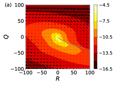
Fixed points and GIMs of the reduced Euler model for a passive scalar in HIT. The method just described gives the so-called Vieillefosse tail or invariant manifold of the QR-model of HIT Vieillefosse (1982), and works with reduced models as those obtained for other flows Sujovolsky et al. (2019); Sujovolsky and Mininni (2020). Now we analyze in detail the fixed points and GIMs of Eq. (9). The Vieillefosse tail $D_{t}(4Q^{3}+27R^{2})=0$ is obtained as a GIM of Eq. (9) for order $n=6$ (note that while the GIMs of the ideal system have free constants of integration, in the presence of forcing and disipation they reduce to finite size basins that go through the origin). Figure 1(a) shows this manifold, as well as the joint probability density function (PDF) of $Q$ and $R$ for the DNS of the full set of partial differential equations (with viscosity and forcing), and also indicates with arrows the evolution in phase space obtained from the time evolution of field gradients along fluid trajectories in the DNS. As is well known for HIT Meneveau (2011), even though the DNS has forcing and dissipation (and the deviatoric part of the pressure Hessian), fluid elements have a larger probability of having $Q$ and $R$ close to the GIM, and also evolve more slowly in the vicinity of this GIM. This provides valuable information on the geometry of the flow structures, as the $Q$-$R$ phase space is divided by the Vieillefosse tail into regions where the flow gradients display different local properties Cantwell (1992); Dallas and Alexakis (2013). In spite of the agreements, we recall that the QR-model has multiple limitations as, e.g., in the QR-model trajectories in phase space diverge in finite time, a process that is arrested in real fluids by pressure gradients and dissipation Chevillard et al. (2008); Wilczek and Meneveau (2014); Johnson and Meneveau (2016); Pereira et al. (2018); Carbone et al. (2020); Parashar et al. (2020).

Figure 3: Logarithm of the joint PDF of $-QS$ and $U$ for (a) only fluid elements in the DNS with $S\approx S_{0}=1$, and (b) all fluid elements. The local invariant manifold $U+QS_{0}=0$ is shown as a reference by the solid line. In (b) we also show $QS=0$ with dashed lines. Arrows show the same as in Figs. 1.

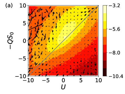
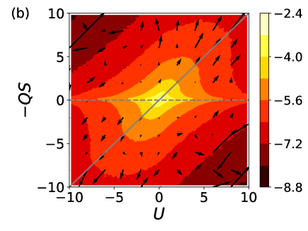
Equation (9) contains the QR-model in its first two equations, and thus it is not a surprise that the Vieillefosse tail is a GIM. Let’s now consider the fixed points and other GIMs and local invariant manifolds of the system (mostly related to the evolution of passive scalar gradients). The fixed points are a GIM by themselves

$$Q=R=T=U=0,\ \ S\ \text{free}.$$ (12)

For any value of $S=S_{0}$ these conditions do not evolve in time, and thus they are an invariant manifold. Physically, they express the fact that gradients of the scalar field do not change if velocity field gradients are zero.

Before, we showed that for order $n=4$

$$D_{t}(4QS^{2}+4SU-T^{2})=0,$$ (13)

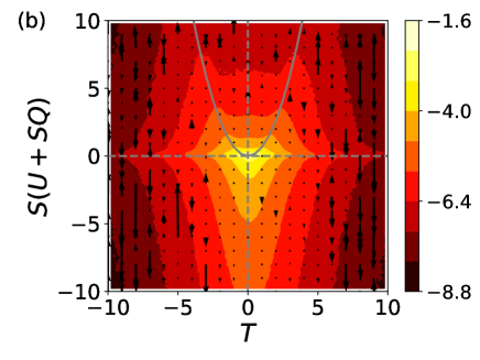
and thus it is a GIM. Figure 1(b) shows the joint PDF of $S(U+SQ)$ and $T$ in the DNS, indicating with a solid line $S(U+SQ)=T^{2}$ (the GIM), as well as $T=0$ and $S(U+SQ)=0$ (which are projections of the fixed points on the plane); note the system phase space has 5 dimensions, and thus the two-dimensional PDFs we show are projections of the total phase space on different planes (this is also the reason why arrows in the figures may overlap). We again see larger probabilities of finding fluid elements near the manifolds. As before, the arrows show the projection of the flow on this plane of phase space obtained from the DNS. The GIMs are not attracting or repelling but arrows become smaller in their vicinity. Note also how the arrows increase as $T$ increases, in agreement with equation $D_{t}S=-T$ in Eq. (9): As $T$ increases, so does the variation of $S$. Physically, this follows from the fact that gradients of the passive scalar ($S$) are stretched and amplified by velocity field gradients ($A_{ij}$).

The third GIM obtained with the method ($n=5$) is

$$D_{t}[9RT-2Q(3U+2QS)]=0.$$ (14)

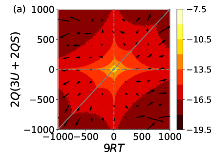
This GIM is shown in Fig. 2, where the solid line indicates $2Q(3U+2QS)=9RT$, and the dashed lines again indicate projections of Eq. (12) on this plane. The accumulation in this GIM becomes more clear when we restrict the DNS data to fluid elements outside the manifold in Eq. (12). Again, the velocity reduces as it goes near the GIM (see the arrows), and there is a larger probability of finding fluid elements in the DNS in the vicinity of these manifolds. Interestingly, the arrows align with the GIM, and escape from zero following this manifold. This behaviour resembles that of the Vieillefosse tail.

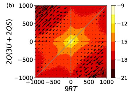
Finally, the system has a local central invariant manifold in the vicinity of the fixed points. When the system is linearized around Eq. (12), it can be shown that $U+QS_{0}=0$ is an invariant manifold, where $S_{0}$ is a fixed (constant) value of $S$. Figure 3 shows the $QS$ vs. $U$ plane for fluid elements with $S_{0}\approx 1$, and for all fluid elements in the DNS. The invariant manifold, and the projection of $Q=S=0$ on this plane are marked by solid and dashed lines respectively. Again an accumulation of fluid elements and a slow down in the dynamics can be seen in the DNS in the vicinity of the manifolds. Interestingly this indicates that $S$ (i.e., the passive scalar gradients) can remain approximately constant for a while when $S\approx-U/Q$ locally in the flow.

Discussion. We presented a reduced model for the evolution of passive scalar gradients in HIT, and a method to identify GIMs with algebraic expressions in nonlinear ODEs. Such GIMs often arise and play a relevant role, e.g., in reduced models for field gradients in fluids Vieillefosse (1982); Cantwell (1992); Li and Meneveau (2005); Chevillard and Meneveau (2006); Meneveau (2011); Johnson and Meneveau (2016); Pereira et al. (2018); Sujovolsky et al. (2019), where the persistence of low dimensional structures in complex and out-of-equilibrium flows is in many cases associated with the GIMs’ existence. In such models, an important problem is how to improve approximations for the treatment of the pressure Hessian Chevillard et al. (2008); Wilczek and Meneveau (2014); Carbone et al. (2020); Parashar et al. (2020), but treatment of systems with more degrees of freedom than HIT as often appear in more realistic flows also faces the problem of how to find invariant manifolds and to characterize phase space as the complexity of the reduced system increases Girimaji and Speziale (1995); Li (2010); Pumir (2017); Sujovolsky et al. (2019); Sujovolsky and Mininni (2020). In this case, as well as for other ODEs with GIMs with algebraic expressions, the method presented here can be of some value.

Moreover, the reduced model derived for the passive scalar in Eq. (12) has two autonomous ODEs for the isotropic invariants of the velocity field gradients ($Q$ and $R$) which are the usual QR-model Vieillefosse (1982); Cantwell (1992); Meneveau (2011), and three ODEs for the evolution of the gradients of the passive scalar (the equations for $S$, $T$, and $U$). It is remarkable that a closed system of 3 ODEs can be derived for the gradients of the scalar, which is only limited by the approximation of neglecting diffusivity (as the pressure Hessian does not affect the evolution of $\theta$). These ODEs and their manifolds capture the well know physics of the problem. Passive scalar gradients remain the same in the absence of velocity field gradients, and are amplified by strain in the velocity. The growth of $S$ along these manifolds is also consistent with recent observations of ramp-cliff structures in scalar turbulence. Other manifolds are non-trivial as, e.g., the fact that $S$ anti-correlates with $U/Q$, or the existence of other correlations of even higher order (in the nonlinearity) between velocity field and scalar gradients. Extensions of this model can be used to consider the problem of intermittency in the passive scalar Celani et al. (2000); Watanabe and Gotoh (2007); Buaria et al. (2021). The effect of diffusivity can be also included: its role should be to shrink the volume that orbits in phase space can explore, thus allowing studies of the effect of the Schmidt number in passive scalar turbulence.

The authors acknowledge fruitful discussions with G.B. Mindlin and D.J. Seidler, and support from PICT Grant No. 2015-3530 and 2018-4298, and of grant UBACyT No. 20020170100508.

References

- Lorenz (1963) E. N. Lorenz, J. Atm. Sci. 20, 130 (1963).
- Holmes et al. (1996) P. Holmes, J. L. Lumley, and G. Berkooz, Turbulence, Coherent Structure, Dynamical Systems and Symmetry (Cambridge Univ. Press, 1996).
- Li and Meneveau (2005) Y. Li and C. Meneveau, Phys. Rev. Lett. 95, 164502 (2005).
- Chevillard and Meneveau (2006) L. Chevillard and C. Meneveau, Phys. Rev. Lett. 97, 174501 (2006).
- Meneveau (2011) C. Meneveau, Annu. Rev. Fluid Mech. 43, 219 (2011).
- Johnson and Meneveau (2016) P. L. Johnson and C. Meneveau, J. Fluid Mech. 804, 387 (2016).
- Pereira et al. (2018) R. M. Pereira, L. Moriconi, and L. Chevillard, J. Fluid Mech. 839, 430 (2018).
- Sujovolsky et al. (2019) N. E. Sujovolsky, G. B. Mindlin, and P. D. Mininni, Phys. Rev. Fluids 4, 052402 (2019).
- Vieillefosse (1982) P. Vieillefosse, J. Physique 43, 837 (1982).
- Guckenheimer and Holmes (1983) J. Guckenheimer and P. Holmes, Nonlinear Oscillations, Dynamical Systems and Bifurcations of Vector Fields (Springer, 1983).
- Celani et al. (2000) A. Celani, A. Lanotte, A. Mazzino, and M. Vergassola, Phys. Rev. Lett. 84, 2385 (2000).
- Watanabe and Gotoh (2007) T. Watanabe and T. Gotoh, J. Fluid Mech. 590, 117 (2007).
- Buaria et al. (2021) D. Buaria, M. P. Clay, K. R. Sreenivasan, and P. Yeung, Phys. Rev. Lett. 126, 034504 (2021).
- Shraiman and Siggia (2000) B. I. Shraiman and E. D. Siggia, Nature 405, 639 (2000).
- Falkovich et al. (2001) G. Falkovich, K. Gawȩdzki, and M. Vergassola, Rev. Mod. Phys. 73, 913 (2001).
- Donzis and Yeung (2010) D. Donzis and P. Yeung, Physica D 239, 1278 (2010).
- Gotoh and Watanabe (2015) T. Gotoh and T. Watanabe, Phys. Rev. Lett. 115, 114502 (2015).
- Mininni et al. (2011) P. D. Mininni, D. Rosenberg, R. Reddy, and A. Pouquet, Parallel Comp. 37, 316 (2011).
- Yeung and Pope (1988) P. K. Yeung and S. B. Pope, J. Comp. Phys. 79, 373 (1988).
- Cantwell (1992) B. J. Cantwell, Phys. Fluids A 4, 782 (1992).
- Wilczek and Meneveau (2014) M. Wilczek and C. Meneveau, J. Fluid Mech. 756, 191 (2014).
- Carbone et al. (2020) M. Carbone, M. Iovieno, and A. D. Bragg, J. Fluid Mech. 900 (2020).
- Parashar et al. (2020) N. Parashar, B. Srinivasan, and S. S. Sinha, Phys. Rev. Fluids 5, 114604 (2020).
- Chevillard et al. (2008) L. Chevillard, C. Meneveau, L. Biferale, and F. Toschi, Phys. Fluids 20, 101504 (2008).
- Sujovolsky and Mininni (2020) N. E. Sujovolsky and P. D. Mininni, Phys. Rev. Fluids 5, 064802 (2020).
- Dallas and Alexakis (2013) V. Dallas and A. Alexakis, Phys. Fluids 25, 105106 (2013).
- Girimaji and Speziale (1995) S. S. Girimaji and C. G. Speziale, Phys. Fluids 7, 1438 (1995).
- Li (2010) Y. Li, Physica D 239, 1948 (2010).
- Pumir (2017) A. Pumir, Phys. Rev. Fluids 2, 074602 (2017).