Confinement-induced zero-bias peaks in conventional superconductor hybrids

Abstract

Majorana bound states in topological superconductors have been predicted to appear in the form of zero-bias conductance peaks of height $2e^{2}/h$, which represents one of the most studied signatures so far. Here, we show that quasi zero-energy states, similar to Majorana bound states, can naturally form in any superconducting hybrid junction due to confinement effects, without relation to topology. Remarkably, these topologically trivial quasi zero-energy states produce zero-bias conductance peaks, thus mimicking the most representative Majorana signature. Our results put forward confinement as an alternative mechanism to explain the ubiquitous presence of trivial zero-bias peaks and quasi zero-energy states in superconductor hybrids.

Introduction.—The realization of topological superconductivity featuring Majorana bound states (MBSs) in superconducting hybrid systems has lately been the subject of intense research due to its potential for technological applications [1, 2, 3, 4, 5, 6, 7, 8]. The most promising approach involves semiconductor nanowires with strong spin-orbit coupling and proximity-induced conventional superconductivity [9, 10]. Here, an external magnetic field drives such systems into a topological phase where MBSs emerge at zero energy and localize at each end of the wire. These properties enable MBSs to form the basis for qubit proposals robust against local perturbations [11, 12, 13, 14, 15, 16], highlighting the importance of topological superconductivity in condensed matter physics.

The detection of MBSs has been mainly pursued by exploiting their zero-energy nature. Indeed, tunneling from a normal metal into a MBS has been predicted to result in a zero-bias conductance peak (ZBCP) of height $2e^{2}/h$ [17, 18, 19, 20, 21, 22]. Subsequently, many experiments reported ZBCPs and interpreted them as strong evidence of MBSs [23, 24, 25, 26, 27, 28, 29, 30, 31]. Despite the significant experimental progress, the Majorana origin of ZBCPs has been recently questioned. In great part because several works have reported ZBCPs due to quasi zero-energy states (qZESs) at finite magnetic fields but well below the topological phase and, hence, not tied to topology [32, 33, 34, 35, 36, 37, 38, 39, 40, 41, 42, 43, 44, 45, 46, 47, 48, 49, 50, 51, 52]. In this regard, recent theoretical efforts have suggested interesting detection protocols of MBSs [53, 54, 55, 56, 57, 58, 59, 60, 61, 62, 63, 64, 65, 66, 67, 68, 69, 70, 71, 72], but the emergence of trivial qZESs still seems puzzling in conductance measurements.

Given the complex experimental setups involved in all Majorana platforms, it is fair to say that it still remains unclear if the emergence of trivial qZESs, and associated ZBCPs, is due to the interplay between superconductivity and magnetism, the intrinsic inhomogeneities of superconducting heterostructures, or both. Understanding the mechanisms behind these non-topological states can help to interpret ZBCPs in experiments, rule out a possible Majorana origin, and envisage routes for mitigating the emergence of the unwanted qZESs.

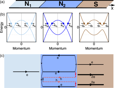
Figure 1: (a) Sketch of a one-dimensional N₁N₂S junction. (b) Dispersion relation on each region at the same chemical potential. The arrows represent the velocity direction of electrons and holes with wavevectors $k_{e,h}$ in N_1,2 and $q_{e,h}$ in S. (c) Quasi-bound states in N₂ involving only normal reflections (top) or both normal and Andreev processes (bottom).

In this work we demonstrate that qZESs can naturally emerge in hybrid junctions with conventional $s$-wave superconductors just due to confinement, and thus requiring neither magnetism nor spin-orbit coupling. To illustrate this generic effect, we consider a normal metal-normal metal-superconductor (N₁N₂S) junction, as in Fig. 1(a), where confinement in the central region (N₂) enables the formation of qZESs. Interestingly, we find that these trivial qZESs produce almost perfectly quantized ZBCPs that mimic those due to MBSs. Since most of the setups used to detect MBSs are prone to confinement, the emergence of topologically trivial qZESs, with quantized ZBCPs, is a generic and ubiquitous effect in any superconducting hybrid system.

Theoretical formulation.—We consider a ballistic one-dimensional junction between a normal metal and a superconductor separated by a normal region of length $L$, as shown in Fig. 1(a). This can be modeled by the Bogoliubov-de Gennes (BdG) Hamiltonian given by,

$$H=\bigg{[}\frac{p^{2}}{2m}-\mu(x)\bigg{]}\tau_{z}+\Delta(x)\tau_{x},$$ (1)

where $p=-i\hbar\partial_{x}$ is the momentum operator, $m$ the electron effective mass, $\mu(x)=\mu_{\rm N_{1}}\Theta(-x-L)+\mu_{\rm N_{2}}\theta(x+L)\Theta(-x)+\mu_{\rm S}\Theta(x)$ represents the chemical potential profile across the junction, with $\Theta(x)$ being the Heaviside step function and $\mu_{\rm N_{1(2)}}$ and $\mu_{\rm S}$ the chemical potentials in $N_{1(2)}$ and S regions, respectively. Moreover, $\Delta(x)=\Delta\Theta(x)$ represents the conventional singlet $s$-wave pair potential with $\Delta\neq 0$ only in S. We contrast our findings with junctions where S is a topological superconductor, which we model substituting the pair potential in Eq. 1 by the spin-triplet $p$-wave $\Delta(x)=\operatorname{sgn}(p)\Delta\Theta(x)$ [73].

Diagonalizing the Hamiltonian in Eq. 1, we obtain the energy-momentum dispersion in each region presented in Fig. 1(b), with wavevectors in the N regions given by $k_{e_{i},h_{i}}=k_{\rm N_{i}}\sqrt{1\pm\omega/\mu_{\rm N_{i}}}$, with $k_{\rm N_{i}}=\sqrt{2m\mu_{\rm N_{i}}/\hbar^{2}}$ and $i=1,2$. In the S region, we obtain $q_{e,h}=k_{\rm S}\sqrt{1\pm\sqrt{\omega^{2}-\Delta^{2}}/\mu_{\rm S}}$, with $k_{\rm S}=\sqrt{2m\mu_{\rm S}/\hbar^{2}}$. These wavevectors characterize the right and left moving electrons and holes (electron-like and hole-like quasiparticles) in the normal (superconducting) regions, indicated by filled circles with horizontal arrows in Fig. 1(b). Next, we use the scattering states associated to these quasiparticles to show how confinement in the middle region enables the formation of qZESs.

Confinement in normal-state junctions.—To understand the origin and impact of confinement in hybrid junctions modeled by Eq. 1, we first inspect the role of the intermediate N₂ region on transport across the junction when S is in its normal state (i.e., $\Delta=0$). For this purpose, we calculate the normal transmission across the NN₂N junction by matching the scattering states at the system interfaces, obtaining

$$T_{\rm N}=\frac{2e^{2}/h}{1+\big{[}\frac{k_{e}}{2k_{e_{2}}}+\frac{k_{e_{2}}}{2k_{e}}\big{]}^{2}-\big{[}\frac{k_{e}}{2k_{e_{2}}}-\frac{k_{e_{2}}}{2k_{e}}\big{]}^{2}{\rm cos}(2k_{e_{2}}L)},$$ (2)

where, without loss of generality, we assumed that the outer regions have the same chemical potential $\mu$ (i.e., $k_{e1}=q_{e}\equiv k_{e}$), while N₂ has $\mu_{\rm N_{2}}$ and length $L$. For a detailed derivation of Eq. 2, see Supplementary Material (SM) [74]. The normal transmission $T_{\rm N}$, Eq. 2, describes the possibility of an incident electron to be transmitted through the junction after experiencing several normal reflections inside the middle N₂ region. The effect of N₂ is captured in the cosine term in the denominator of Eq. 2, which signals the appearance of confinement and enables the formation of discrete energy levels whose number depends on the length of N₂, similarly to a Fabry-Perot cavity. Consequently, there is a resonant transmission $T_{\rm N}/(e^{2}/h)=1$ either in the absence of N₂, i.e., for $L=0$ which leads to $\cos(2k_{e_{2}}L)=1$, or when the wave vectors of the three regions are the same, $k_{e}=k_{e_{2}}$, see Fig. 1(b). For a finite length N₂ region, with a chemical potential different than the outer regions, the resonant condition is $k_{e_{2}}L=n\pi$, with $n$ and integer.

To visualize this behavior, we plot $T_{\rm N}$ in Fig. 2(a) as a function of the chemical potential $\mu_{\text{N}2}$. This allows us to identify the conditions for transport on and off resonance when the transmission is either maximum [$T_{\rm N}/(e^{2}/h)=1$] or minimum. On resonance, we obtain a ZBCP with periodicity determined by the length $L$, cf. Eq. 2. Interestingly, $T_{\rm N}$ can be resonant at exactly zero energy ($\omega=0$), that is, solely as a result of confinement from the middle region due to the finite length and different chemical potential, see dashed line in Fig. 2(a); see also Fig. 2(b). As we show next, this rather general result is behind the formation of trivial Andreev qZESs in superconducting junctions, making this effect ubiquitous in superconducting heterostructures [75].

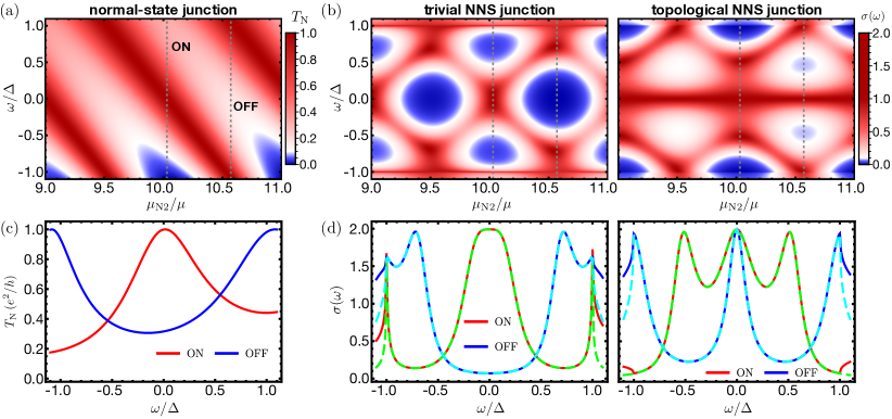
Figure 2: (a,b) Map of the conductance as a function of energy and the chemical potential of the intermediate region N₂ for a junction in the normal state (a) or with a trivial and topological superconductor (b). (c,d) Conductance on and off-resonance when the junction is in the normal state (c) or has a trivial or a topological superconductor (d). The values of $\mu_{\text{N}2}$ for each case are plotted as dashed gray lines in the maps, labeled ON and OFF for on- and off-resonance, respectively. For (d), we plot $2|r_{eh}|^{2}$ using green (cyan) dashed lines for on (off) resonance. In all cases, $k_{\text{F}}L=3\pi/2$, $\mu_{N1}=\mu_{S}\equiv\mu=2\Delta$.

Confinement in superconducting junctions.—We now analyze the consequences of confinement in transport across trivial and topological N₁N₂S junctions. In addition to normal reflections at both interfaces, Andreev reflections also take place at the N₂S interface, where incident electrons from N₂ are reflected back as holes [76]. Owing to these Andreev reflections the discrete energy levels of the middle region, discussed in previous section, become coherent superpositions of electrons and holes. As a result, Andreev quasi-bound states are formed with properties that depend on the system parameters, as schematically shown by the bottom process of Fig. 1(c). This occurs for both trivial and topological junctions. To analyze the impact of this phenomenon on transport properties, we inspect the normalized conductance [77]

$$\sigma(\omega)=\frac{2e^{2}}{h}T_{\text{N}}^{-1}(1-|r_{ee}(\omega)|^{2}+|r_{eh}(\omega)|^{2})\,,$$ (3)

where $T_{\text{N}}$ is given by Eq. 2, and $r_{ee}$ and $r_{eh}$ represent the normal and Andreev reflection amplitudes, respectively. These amplitudes are obtained by matching the scattering states of Eq. 1 at the interfaces of the N₁N₂S junction [74]. Equation 3 characterizes transport in both trivial and topological junctions, and we now discuss how it is affected by confinement effects.

In Fig. 2(b) we map the conductance $\sigma$ as a function of the energy $\omega$ and the chemical potential of the middle region $\mu_{\rm N_{2}}$ for a trivial and a topological (right panel) N₁N₂S junction. For both trivial and topological junctions, the conductance develops resonances with maximum values (dark red areas) that double those obtained when S is in its normal state, see Fig. 2(a). Here, the most important feature is that the conductance for a trivial N₁N₂S junction exhibits a ZBCP for exactly the same parameters that result in a resonant normal-state transmission, see Fig. 2. Note that the appearance of this ZBCP can be tuned by the chemical potential of the middle region $\mu_{\text{N}2}$. We have verified that impurity scattering at the interfaces narrows the width of this ZBCP. The presence or absence of a ZBCP directly corresponds to the on- or off-resonance regimes of the normal-state conductance, marked by vertical dotted lines in Fig. 2(a,b). By contrast, the ZBCP in topological junctions remains robust for any value of $\mu_{\text{N}2}$. On resonance, however, it can be challenging to identify whether the ZBCP is of trivial or topological nature as in both cases it exhibits a very similar behavior.

On resonance, the ZBCP for a trivial superconductor is properly quantized as twice the normal state transmission, compare Fig. 2(c) and Fig. 2(d). Such quantization quickly disappears if $\mu_{\text{N}2}$ is tuned out of resonance. Moreover, the ZBCP is mainly due to Andreev processes fulfilling $\sigma(|\omega|<\Delta)=2|r_{eh}|^{2}$, with $|r_{eh}(\omega=0)|^{2}\rightarrow 1$, see green and cyan dashed lines in Fig. 2(d). By contrast, the topological superconductor features a ZBCP both on and off resonance, with a perfect zero energy Andreev reflection $|r_{eh}(\omega=0)|^{2}=1$. While topological junctions exhibit robust unitarity of Andreev reflection, confinement in trivial junctions can only approximately accommodate regimes of unitarity. These two situations are, however, difficult to distinguish by naked eye.

The findings discussed above thus show that, on-resonance, the ZBCPs for both trivial and topological junctions feature a very similar behavior. We stress again that the ZBCP for trivial junctions arises solely due to confinement effects of the central region, since we have not considered any magnetic order and the pair potential does not include MBSs. Consequently, a ZBCP is not a definitive indicator of MBSs or topological superconductivity as it can easily appear in ballistic heterostructures without magnetic order or topology.

Real space zero-energy LDOS.—To better understand the behavior of the trivial qZES, we now study the spatial dependence of the local density of states (LDOS) $\rho$ at zero-energy. The LDOS is obtained from the retarded Green’s function $G^{r}(x,x^{\prime},\omega)$ associated to the BdG Hamiltonian in Eq. 1. To find $G^{r}(x,x^{\prime},\omega)$ we follow a scattering Green’s function approach [74] commonly used for superconducting junctions [78, 79, 17, 80, 81, 82, 83, 84]. The Green’s function $G^{r}(x,x^{\prime},\omega)$ is a $2\times 2$ matrix in Nambu (particle-hole) space, and the LDOS is then obtained as $\rho(\omega,x)=-{\rm Im}{\rm Tr}[G^{r}(x,x,\omega)]/\pi$. The LDOS in S and N₂ exhibits a complex behavior, but in N₁ it is simply given by

$$\rho(\omega,x)=\frac{m}{\pi\hbar^{2}}{\rm Im}\Big{\{}\sum\limits_{\alpha=e,h}\frac{i}{k_{\alpha}}\left(1+r_{\alpha\alpha}{\rm e}^{-2is_{\alpha}k_{\alpha}x}\right)\Big{\}},$$ (4)

where $s_{e,h}=\pm 1$ and $r_{\alpha\alpha}$ represent normal reflection amplitudes. Deep inside the leftmost normal region, the LDOS adopts the simple form $\rho_{0}=m(k^{-1}_{e1}+k^{-1}_{h1})/(\pi\hbar^{2})$, which we use for normalization.

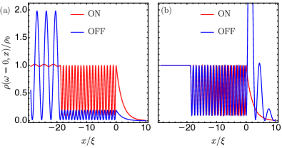
Figure 3: Spatial dependence of the zero-energy LDOS for trivial (a) and topological (b) junctions, with the same parameters as Fig. 2, and red (blue) lines corresponding to on- (off-)resonance.

Because our interest is on the qZES, we present in Fig. 3 the spatial dependence of the zero-energy LDOS for trivial (a) and topological (b) junctions, when the chemical potential of the middle region $\mu_{\rm N_{2}}$ is set on- and off-resonance (red and blue lines, respectively). For topological junctions, Fig. 3(b), the zero-energy LDOS is almost independent of the chemical potential in N₂, $\mu_{\rm N_{2}}$. The zero-energy LDOS is perfectly flat on N₁ and oscillates with constant amplitude in N₂, unaffected by variations of $\mu_{\rm N_{2}}$. Both features are a result of the perfect Andreev reflection taking place at the N₂-S interface for $\omega=0$, where the MBS is located, which, in turn, also promotes a perfect transmission at N-N₂. As a result, $r_{ee}=0$ in Eq. 4 and the zero-energy LDOS in N takes exactly the value of the bulk density $\rho_{0}$. Hence, the robust profile of the zero-energy LDOS in topological junctions can be attributed to the presence of a MBS.

For trivial junctions on-resonance, the magnitude and oscillations of the zero-energy LDOSred curve in Fig. 3(a) are very similar to those of topological junctions, albeit there are no MBS present in this case. This indicates the formation of an extended qZES in N₂, which is responsible for the finite LDOS at zero energy at the N-N₂ interface and causes the ZBCP in the conductance on-resonance (Fig. 2). However, off-resonance, the zero-energy LDOS oscillations become vanishing small, as seen in the blue curve of Fig. 3(a). Moreover, the zero-energy LDOS displays clear oscillations in the leftmost normal region N₁, originating from the term proportional to $r_{\alpha\alpha}$ in Eq. 4. While the oscillations in N₁ are present both on- and off-resonance, their amplitude is greatly suppressed on-resonance because normal reflections are finite but vanishing small, i.e., $|r_{ee}|^{2}\rightarrow 0$.

By the exposed above, the zero-energy LDOS on-resonance for a trivial junction has the same qualitative behavior as that of a topological junction. While for trivial junctions on resonance the unitarity of the Andreev reflection is only approximately true, i.e., $|r_{eh}|^{2}\rightarrow 1$, the presence of a MBS in topological junctions promotes a perfect Andreev reflection $|r_{eh}|^{2}=1$. However, whether the Andreev reflection unitarity is approximated or exact is rather challenging to distinguish in measurements, thus posing a critical question when interpreting ZBCPs. Consequently, discerning between the perfect Andreev reflection ($|r_{eh}|^{2}=1$) for a MBS and the approximate one ($|r_{eh}|^{2}\lesssim 1$) for a trivial qZES on resonance would require a very sensitive scanning tunneling experiment.

Finite-size effects.—To showcase the emergence of confinement-induced qZESs, we have thus far considered a perfectly one-dimensional ballistic junction with semi-infinite outer leads. We now explore possible deviations from having finite-size outer leads or quasi-one dimensional junctions. First, we performed tight-binding simulations on finite length systems, after discretizing Eq. 1 on a lattice, and verified that the main findings remain robust under more realistic conditions, see Ref. [74] for more details. Previously, the appearance of trivial qZESs has been confirmed in junctions with spin-orbit coupling and magnetism [34, 70]. However, these junctions require that the middle region is within the helical regime, and it was not clearly determined if the qZESs originate due to confinement or helicity. Our work thus clarifies the pivotal role of confinement in the formation of qZESs in semiconductor hybrid junctions.

Another finite-size effect is related to the finite cross section of semiconducting junctions. Indeed, the Majorana condition in these setups is only fulfilled by a few transverse modes [85]. Even though a perfect one-dimensional regime is challenging to achieve, most Majorana platforms attempt to approach a one-dimensional limit by reducing the number of transverse modes contributing to transport. To study the impact of extra transport modes on the trivial ZBCP, we extend Eq. 1 to describe a two-dimensional system and denote as $k_{y}$ the wavevector component parallel to the interfaces [74]. The transport observables in Eqs. 2 and 3 must then be averaged over all incident modes, and the resonant condition for the confined states in N₂ becomes more complicated, as it now depends on the transverse wavevector $k_{y}$. Consequently, as we add extra modes, the magnitude of the ZBCP for trivial junctions on resonance is reduced, although the peak never disappears. Even though a quantization of the ZBCP in planar junctions is no longer possible, a conductance approaching the quantized value is still achievable in quasi-one dimensional trivial junctions, see Ref. [74].

Conclusions.—We have shown that quasi zero-energy Andreev states can naturally emerge due to confinement effects in hybrid junctions based on conventional $s$-wave superconductors in the absence of any magnetic order. Such confinement-induced states can mimic the behavior of Majorana zero modes, featuring zero-bias conductance peaks and enhanced zero-energy local density of states. Confinement, which here emerges from a depleted or gated finite-length intermediate region, is a very common effect in hybrid junctions, including most Majorana nanowire experiments. Our results thus exemplify how ubiquitous trivial zero-bias peaks can be in hybrid junctions, even without spin fields, and highlight that zero-bias conductance peaks cannot be solely taken as a definitive indicator of Majorana bound states or topological superconductivity.

We thank A. M. Black-Schaffer for insightful discussions. J. C. acknowledges support from C.F. Liljewalchs stipendiestiftelse Foundation, the Knut and Alice Wallenberg Foundation through the Wallenberg Academy Fellows program, and the EU-COST Action CA-16218 Nanocohybri. P. B. acknowledges support from the Spanish CM “Talento Program” No. 2019-T1/IND-14088.

I Supplemental Material for “Confinement-induced zero-bias peaks in conventional superconductor hybrids”

In this Supplementary Material we provide details on how we calculate the conductance, the Green’s functions, and the LDOS for N₁N₂S junctions. We also detail the numerical simulations for finite-size and quasi-one dimensional systems.

II Conductance and density of states

In the main text, we have demonstrated that zero-energy states ubiquitously emerge in finite length junctions due to confinement effects. We have also shown that these zero-energy states give rise to zero-bias conductance peaks and large zero-bias LDOS. To support those findings, here we provide further details on the used models, and on how to obtain conductance and LDOS by using scattering states.

II.1 Junction models

We consider ballistic N₁N₂S junctions, where the middle region N₂ is of finite length $L$, with the left interface located at $x=-L$ and the right interface at $x=0$. The BdG Hamiltonian presented in the main text for the junction with a conventional $s$-wave spin-singlet superconductor can be written as

$$\begin{split}H_{\rm BdG}(x)&=\begin{pmatrix}H_{0}(x)&\Delta(x)\\ \Delta^{\dagger}(x)&-H_{0}(x)\end{pmatrix}\,,\end{split}$$ (S 1)

in the basis $\psi_{k}^{\rm T}=(c_{k,\uparrow},c_{-k,\downarrow}^{\dagger})$, where $H_{0}(x)=\frac{p^{2}}{2m}-\mu(x)$, with $p=-i\hbar\partial_{x}$. For the considered N₁N₂S junction, the $s$-wave spin-singlet pair potential is given by

$$\Delta(x)=\begin{cases}0\,,&x<-L,\\ 0\,,&-L<x<0,\\ \Delta\,,&x>0\,.\end{cases}$$ (S 2)

The chemical potential profile is given by

$$\mu(x)=\begin{cases}\mu_{\rm N_{1}}\,,&x<-L,\\ \mu_{\rm N_{2}}\,,&-L<x<0,\\ \mu_{\rm S}\,,&x>0.\end{cases}$$ (S 3)

To compare our results with unconventional superconductors, we also consider N₁N₂S junctions with S being a topological superconductor. In this case, the modeling is very similar with the difference that S here represents an spinless (spin-polarized) $p$-wave superconductor deep in the topological phase, as in the topological phase of the well known Kitaev model [11]. Hence, S is modelled by a BdG Hamiltonian similar to Eq. (S 1) but now in the spinless basis $\psi_{k}^{\rm T}=(c_{k},c_{-k}^{\dagger})$ and with the order parameter given by $p\Delta/k_{\rm S}$, with $k_{\rm S}$ the Fermi wave vector in S. The N regions are here spin-polarized or spinless, a property shared with the S region as well; this is expected for a strong magnetic field applied along the wire needed to reach the topological phase in the S region based on the conventional realizations of topological superconductivity [3].

II.2 Scattering states

We now discuss how to obtain the conductance and LDOS based on the scattering states for the Bogoliubov-de Gennes (BdG) Hamiltonian given by Eq. (S 1). In order to construct the scattering states, we first solve the eigenvalue problem in each region (N_i and S) by using the Hamiltonian given by Eq. (S 1). Next, we construct the scattering states taking into account right-moving electrons and holes from the leftmost region (N₁) and left-moving quasielectrons and quasiholes from the rightmost region (S). The resulting four scattering processes for the N₁N₂S junction are given by

$$\begin{split}\Psi_{1}(x)&=\begin{cases}\phi_{1}^{\rm N}\,{\rm e}^{ik_{e_{1}}x}+a_{1}\phi_{3}^{\rm N}\,{\rm e}^{ik_{h_{1}}x}+b_{1}\phi_{2}^{\rm N}\,{\rm e}^{-ik_{e_{1}}x},\,\quad\quad\,\,\,\quad\quad\quad\quad\quad\quad\quad\quad\quad x<-L&\\ e_{1}\phi_{1}^{\rm N}\,{\rm e}^{ik_{e_{2}}x}+e_{2}\phi_{2}^{\rm N}\,{\rm e}^{-ik_{e_{2}}x}+e_{3}\phi_{3}^{\rm N}\,{\rm e}^{ik_{h_{2}}x}+e_{4}\phi_{4}^{\rm N}\,{\rm e}^{-ik_{h_{2}}x}\,,\quad\quad\,\,\,-L<x<0&\\ c_{1}\phi_{1}^{\rm S}\,{\rm e}^{iq_{e}x}+d_{1}\phi_{4}^{\rm S}\,{\rm e}^{-iq_{h}x},\,\quad\quad\quad\quad\quad\quad\quad\quad\quad\quad\quad\quad\quad\quad\quad\quad\quad\quad\,x>0&\end{cases},\\ \Psi_{2}(x)&=\begin{cases}\phi_{4}^{\rm N}\,{\rm e}^{-ik_{h_{1}}x}+a_{2}\phi_{2}^{\rm N}\,{\rm e}^{-ik_{e_{1}}x}+b_{2}\phi_{3}^{\rm N}\,{\rm e}^{ik_{h_{1}}x},\quad\quad\quad\quad\quad\quad\quad\quad\quad\quad\quad x<-L&\\ f_{1}\phi_{1}^{\rm N}\,{\rm e}^{ik_{e_{2}}x}+f_{2}\phi_{2}^{\rm N}\,{\rm e}^{-ik_{e_{2}}x}+f_{3}\phi_{3}^{\rm N}\,{\rm e}^{ik_{h_{2}}x}+f_{4}\phi_{4}^{\rm N}\,{\rm e}^{-ik_{h_{2}}x}\,,\quad\quad\,\,-L<x<0&\\ c_{2}\phi_{4}^{\rm S}\,{\rm e}^{-iq_{h}x}+d_{2}\phi_{1}^{\rm S}\,{\rm e}^{iq_{e}x},\,\quad\quad\quad\quad\quad\quad\quad\quad\quad\quad\quad\quad\quad\quad\quad\quad\quad\quad\,x>0&\end{cases},\\ \Psi_{3}(x)&=\begin{cases}c_{3}\phi_{2}^{\rm N}\,{\rm e}^{-ik_{e_{1}}x}+d_{3}\phi_{3}^{\rm N}\,{\rm e}^{ik_{h_{1}}x},\,\quad\quad\quad\quad\quad\quad\quad\quad\quad\quad\quad\quad\quad\quad\quad\quad\,x<-L&\\ g_{1}\phi_{1}^{\rm N}\,{\rm e}^{ik_{e_{2}}x}+g_{2}\phi_{2}^{\rm N}\,{\rm e}^{-ik_{e_{2}}x}+g_{3}\phi_{3}^{\rm N}\,{\rm e}^{ik_{h_{2}}x}+g_{4}\phi_{4}^{\rm N}\,{\rm e}^{-ik_{h_{2}}x}\,,\quad\quad\,\,-L<x<0&\\ \phi_{2}^{\rm S}\,{\rm e}^{-iq_{e}x}+a_{3}\phi_{4}^{\rm S}\,{\rm e}^{-iq_{h}x}+b_{3}\phi_{1}^{\rm S}\,{\rm e}^{iq_{e}x},\,\quad\quad\quad\quad\quad\quad\quad\quad\quad\quad\quad\quad\quad x>0&\end{cases},\\ \Psi_{4}(x)&=\begin{cases}c_{4}\phi_{3}^{\rm N}\,{\rm e}^{ik_{h_{1}}x}+d_{4}\phi_{2}^{\rm N}\,{\rm e}^{-ik_{e_{1}}x},\,\quad\quad\quad\quad\quad\quad\quad\quad\quad\quad\quad\quad\quad\quad\quad\quad\,x<-L&\\ h_{1}\phi_{1}^{\rm N}\,{\rm e}^{ik_{e_{2}}x}+h_{2}\phi_{2}^{\rm N}\,{\rm e}^{-ik_{e_{2}}x}+h_{3}\phi_{3}^{\rm N}\,{\rm e}^{ik_{h_{2}}x}+h_{4}\phi_{4}^{\rm N}\,{\rm e}^{-ik_{h_{2}}x}\,,\quad\quad-L<x<0&\\ \phi_{3}^{\rm S}\,{\rm e}^{iq_{h}x}+a_{4}\phi_{1}^{\rm S}\,{\rm e}^{iq_{e}x}+b_{4}\phi_{4}^{\rm S}\,{\rm e}^{-iq_{h}x}\,,\quad\quad\quad\quad\quad\quad\quad\quad\quad\quad\quad\quad\quad\,\,\,x>0&\end{cases},\end{split}$$ (S 4)

where

$$\begin{split}\phi_{1,2}^{\rm N}&=\begin{pmatrix}1\\ 0\end{pmatrix},\quad\phi_{3,4}^{\rm N}=\begin{pmatrix}0\\ 1\end{pmatrix},\quad\phi_{1,2}^{\rm S}=\begin{pmatrix}u\\ v\end{pmatrix},\quad\phi_{3,4}^{\rm S}=\begin{pmatrix}\eta v\\ u\end{pmatrix},\end{split}$$ (S 5)

are the spinors of the N_i and S regions, with $\eta=+$ ($\eta=-$) for an $s$-wave ($p$-wave) superconductor. We have used the superconducting coherence factors

$$\begin{split}u=\sqrt{\frac{1}{2}\left(1+\frac{\sqrt{\omega^{2}+\Delta^{2}}}{\omega}\right)},\quad v=\sqrt{\frac{1}{2}\left(1-\frac{\sqrt{\omega^{2}+\Delta^{2}}}{\omega}\right)},\end{split}$$ (S 6)

and

$$\begin{split}k_{e_{i}(h_{i})}=\sqrt{\frac{2m}{\hbar^{2}}\left(\mu_{\rm N_{i}}\pm\omega\right)}\,,\quad q_{e(h)}=\sqrt{\frac{2m}{\hbar^{2}}\left(\mu_{\rm S}\pm\sqrt{\omega^{2}-\Delta^{2}}\right)}\,,\\ \end{split}$$ (S 7)

representing the electron (hole) wavevectors in the normal N₁ and superconducting S regions, respectively.

The four scattering processes $\Psi_{i}$ in Eqs. (S 4) represent, respectively, incident right-moving electron, right-moving hole, left-moving quasi-electron, and left-moving quasi-hole. The coefficients of the scattering states have a very specific meaning, associated to the nature of scattering process they describe. For instance, for $\Psi_{1}$, $a_{1}$ and $b_{1}$ are the amplitude of Andreev and normal reflections in N₁, respectively. Similarly, $c_{1}$ and $d_{1}$ are the amplitude of transmission into a quasielectron and quasihole, respectively.

In order to fully determine the scattering states $\Psi_{i}$ we still need to calculate their coefficients $a_{i}$, $b_{i}$, $c_{i}$, $d_{i}$, $d_{i}$, $e_{i}$, $f_{i}$, $g_{i}$, and $h_{i}$, with $i=1,2,3,4$. This is carried out by using the conditions established when integrating the BdG equations at both interfaces, which read

$$\begin{split}\Big{[}\partial_{x}\Psi(0>x>-L_{\rm N})]-[\partial_{x}\Psi(x<-L_{\rm N})]&=0\,,\\ \Big{[}\partial_{x}\Psi(x>0)]-[\partial_{x}\Psi(x<0)]&=0\,,\\ [\Psi_{i}(x<-L_{\rm N}))]&=[\Psi_{i}(0>x>-L_{\rm N}))]\,,\\ [\Psi_{i}(x<0)]&=[\Psi_{i}(x>0)]\,.\end{split}$$ (S 8)

This way we obtain all the coefficients of the scattering states in Eqs. (S 4), for N₁N₂S junctions with S being either $s$-wave or $p$-wave superconductor deep in the topological phase. Here, junctions with an $s$-wave superconductor are referred to as trivial junctions, while those with a $p$-wave superconductor in the topological phase are referred to as topological junctions.

The coefficients of Eqs. (S 4) allow us to obtain the local conductance in N₁ at zero temperature as,

$$\sigma(\omega)=\frac{2e^{2}}{h}\big{[}1-|b_{1}|^{2}+|a_{1}|^{2}\big{]}\,,$$ (S 9)

where $a$ and $b$ represent the amplitude of Andreev and normal reflection amplitudes, respectively. Note that Eq. (S 9) is valid for both trivial and topological junctions. Eq. S 9 is used to obtain the conductance in Fig. 2 of the main text for trivial and topological junctions.

In the case of a trivial ($\eta=+$) and a topological ($\eta=-$) junction, the normal and Andreev reflection amplitudes are

$$\begin{split}a_{1}={}&-\frac{8\Gamma}{t}k_{e1}k_{e2}k_{h2}\left(q_{e}+q_{h}\right)\mathrm{e}^{-i(k_{e1}-k_{h1}-k_{e2}-k_{h2})L},\\ b_{1}={}&-\frac{1}{t}\left\{\left(k_{e1}+k_{e2}\right)\left(k_{h1}-k_{h2}\right)\left[\left(q_{e}-k_{e2}\right)\left(q_{h}-k_{h2}\right)-\eta\Gamma^{2}\left(q_{h}+k_{e2}\right)\left(q_{e}+k_{h2}\right)\right]\right.\\ &\left.+\left(k_{e1}-k_{e2}\right)\left(k_{h1}+k_{h2}\right)\left[\left(q_{e}+k_{e2}\right)\left(q_{h}+k_{h2}\right)-\eta\Gamma^{2}\left(q_{h}-k_{e2}\right)\left(q_{e}-k_{h2}\right)\right]\mathrm{e}^{-2i(k_{e2}-k_{h2})L}\right.\\ &\left.-\left(k_{e1}-k_{e2}\right)\left(k_{h1}-k_{h2}\right)\left[\left(q_{e}+k_{e2}\right)\left(q_{h}-k_{h2}\right)-\eta\Gamma^{2}\left(q_{h}-k_{e2}\right)\left(q_{e}+k_{h2}\right)\right]\mathrm{e}^{-2ik_{e2}L}\right.\\ &\left.-\left(k_{e1}+k_{e2}\right)\left(k_{h1}+k_{h2}\right)\left[\left(q_{e}-k_{e2}\right)\left(q_{h}+k_{h2}\right)-\eta\Gamma^{2}\left(q_{h}+k_{e2}\right)\left(q_{e}-k_{h2}\right)\right]\mathrm{e}^{2ik_{h2}L}\right\},\\ t={}&\left(k_{e1}+k_{e2}\right)\left(k_{h1}-k_{h2}\right)\left[\left(q_{e}+k_{e2}\right)\left(q_{h}-k_{h2}\right)-\eta\Gamma^{2}\left(q_{h}-k_{e2}\right)\left(q_{e}+k_{h2}\right)\right]\\ +&\left(k_{e1}-k_{e2}\right)\left(k_{h1}+k_{h2}\right)\left[\left(q_{e}-k_{e2}\right)\left(q_{h}+k_{h2}\right)-\eta\Gamma^{2}\left(q_{h}+k_{e2}\right)\left(q_{e}-k_{h2}\right)\right]\mathrm{e}^{2i(k_{e2}+k_{h2})L}\\ -&\left(k_{e1}-k_{e2}\right)\left(k_{h1}-k_{h2}\right)\left[\left(q_{e}-k_{e2}\right)\left(q_{h}-k_{h2}\right)-\eta\Gamma^{2}\left(q_{h}+k_{e2}\right)\left(q_{e}+k_{h2}\right)\right]\mathrm{e}^{2ik_{e2}L}\\ -&\left(k_{e1}+k_{e2}\right)\left(k_{h1}+k_{h2}\right)\left[\left(q_{e}+k_{e2}\right)\left(q_{h}+k_{h2}\right)-\eta\Gamma^{2}\left(q_{h}-k_{e2}\right)\left(q_{e}-k_{h2}\right)\right]\mathrm{e}^{2ik_{h2}L},\end{split}$$ (S 10)

with $\Gamma=|\Delta|/(\omega+\sqrt{\omega^{2}-\Delta^{2}})$.

When superconductivity vanishes, and the leftmost and rightmost regions are normal metals with the same chemical potential, the conductance adopts a simplified form given by

$$T_{\rm N}(\omega)=\frac{2e^{2}}{h}\frac{1}{1+\big{[}\frac{k_{e1}}{2k_{e2}}+\frac{k_{e2}}{2k_{e1}}\big{]}^{2}-\big{[}\frac{k_{e1}}{2k_{e2}}-\frac{k_{e2}}{2k_{e1}}\big{]}^{2}{\rm cos}(2k_{e_{2}}L)}\,.$$ (S 11)

where $k_{e1}$ is the electron wave vector for both the leftmost and rightmost regions, while $k_{e_{2}}$ belongs to the middle one. Equation (S 11) results from the following scattering processes: an incident electron from N₁ can be transmitted through N₂ directly into the rightmost region N₃, or it can be trapped inside the finite region N₂, experience several reflections at both interfaces, and get finally transmitted to $N_{3}$. Consequently, the finite length region N₂ behaves like a cavity, trapping electrons which develop an interference pattern because the incident electronic state has two possible paths through N₂. This effect is reflected in the denominator of $T_{\rm N}$ in the form of an oscillatory cosine function that depends on the properties of the finite middle region N₂. The cosine term thus permits the appearance of discrete energy levels in the finite region. The oscillatory modulation disappears either when $L=0$ (no middle region or an extremely short one), or when we have the same wave vectors in all the three regions, i.e., $k_{e1}=k_{e2}$. The latter case requires the same chemical potentials in all three regions. Whenever one of these two conditions are satisfied we get a normal transmission of $T_{\rm N}=1$, an instance of resonant transport as seen in Fig. S 1(a); see also orange and blue curves in (b) and (c), respectively.

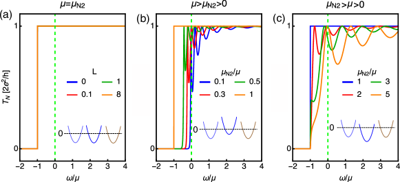
Figure S 1: Conductance of an N₁N₂S junction when S is in the normal state, for (a) equal chemical potentials $\mu=\mu_{\rm N_{2}}>0$, (b) $\mu>\mu_{\rm N_{2}}>0$, and (c) $0<\mu<\mu_{\rm N_{2}}$. The insets depict the position of the bands under the given chemical potentials with respect to zero energy.

Interestingly, the normal-state transmission $T_{\rm N}$ features an energy modulation when the middle region is finite and its chemical potential different from that of the outer regions. The energy modulation can be enhanced when, e.g., we take the limit $0<k_{e1}\ll 2k_{e2}$, where the transmission acquires the following form $T_{\rm N}\approx 2/[1+(k_{e1}^{2}/2k_{e2}^{2}){\rm sin}^{2}(k_{e2}L)]<1$. Analogously, for $0<k_{e2}\ll 2k_{e1}$, we get $T_{\rm N}\approx 2/[1+(k_{e2}^{2}/2k_{e1}^{2}){\rm sin}^{2}(k_{e2}L)]<1$. In these two regimes the transmission is reduced to $T_{\rm N}\ll 1$ when the sine term has maximal amplitude ($\sin^{2}(k_{e2}L)\sim 1$). Figure S 1 shows how the oscillatory modulation tends to reduce the values of the perfect transmission as a result of the phases acquired by the electrons inside the finite region. This effect coincides with the appearance of discrete energy levels inside N₂, which can be seen as resonances of the transmission in Fig. S 1 (b,c). An interesting feature to note in Fig. S 1 (b,c) is that $T_{\rm N}$ can be peaked at zero energy $\omega=0$, solely as a result of the finite length and different chemical potentials. We show in the main text that this innocent behavior has interesting consequences in the physics of hybrid junctions.

The local conductance in the normal state plotted in Fig. S 1 is presented in Eq. (2) of the main text.

II.3 Retarded Green’s functions

We now detail how to obtain the LDOS presented in Eq. (6) and Fig. 3 of the main text. To calculate the LDOS we employ the retarded Green’s function of the system. Thus, we first construct the retarded Green’s function $G^{r}(x,x^{\prime},\omega)$ with outgoing boundary conditions in each region from the scattering processes at the interfaces [86]. Thus, in general, the retarded Green’s function can be calculated as [86, 87]

$$\begin{split}G^{r}(x,x^{\prime},\omega)=&\begin{cases}\alpha_{1}\Psi_{1}(x)\tilde{\Psi}_{3}^{T}(x^{\prime})+\alpha_{2}\Psi_{1}(x)\tilde{\Psi}_{4}^{T}(x^{\prime})+\alpha_{3}\Psi_{2}(x)\tilde{\Psi}_{3}^{T}(x^{\prime})+\alpha_{4}\Psi_{2}(x)\tilde{\Psi}_{4}^{T}(x^{\prime}),&x>x^{\prime},\\ \beta_{1}\Psi_{3}(x)\tilde{\Psi}_{1}^{T}(x^{\prime})+\beta_{2}\Psi_{4}(x)\tilde{\Psi}_{1}^{T}(x^{\prime})+\beta_{3}\Psi_{3}(x)\tilde{\Psi}_{2}^{T}(x^{\prime})+\beta_{4}\Psi_{4}(x)\tilde{\Psi}_{2}^{T}(x^{\prime}),&x<x^{\prime},\end{cases}\end{split}$$ (S 12)

where $\Psi_{i}$ represent the scattering processes at the interfaces of the junction under investigation (N₁N₂S) and given by Eqs. (S 4). Here, $\tilde{\Psi}_{i}$ corresponds to the conjugated scattering processes obtained using $\tilde{H}_{\rm BdG}(k)=H_{\rm BdG}^{*}(-k)=H_{\rm BdG}^{\rm T}(-k)$ instead of Eq. (S 1). In general, the component of $\Psi_{i}$ (either for N_i or S) used will determine the range of $x$ and $x^{\prime}$.

The coefficients $\alpha_{i}$ and $\beta_{i}$ in Eq. (S 12) are found from the continuity of the Green’s function

$$[\omega-H_{\rm BdG}(x)]G^{r}(x,x^{\prime},\omega)=\delta(x-x^{\prime})\,,$$ (S 13)

where $H_{\rm BdG}$ is the BdG Hamiltonian of the system defined in Eq. (S 1). Then, by integrating around $x=x^{\prime}$ we obtain

$$\begin{split}&[G^{r}(x>x^{\prime})]_{x=x^{\prime}}=[G^{r}(x<x^{\prime})]_{x=x^{\prime}}\,,\\ &[\partial_{x}G^{r}(x>x^{\prime})]_{x=x^{\prime}}-[\partial_{x}G^{r}(x<x^{\prime})]_{x=x^{\prime}}=(2m/\hbar^{2})\tau_{z}\,,\end{split}$$ (S 14)

where $\tau_{i}$ are $i$-Pauli matrices in electron-hole space.

In general, the Green’s function, either in N_i or S region, is a $2\times 2$ matrix in electron-hole space,

$$G^{r}(x,x^{\prime},\omega)=\begin{pmatrix}G^{r}_{0}(x,x^{\prime},\omega)&F(x,x^{\prime},\omega)\\ \bar{F}(x,x^{\prime},\omega)&\bar{G}^{r}_{0}(x,x^{\prime},\omega)\end{pmatrix}\,,$$ (S 15)

where $G^{r}_{0}$ and $F$ correspond to the normal and anomalous components, respectively. Note that each element in the previous matrix is a scalar number because spin is not active. The diagonal term $G_{0}^{r}$ is particularly relevant because it allows us to calculate the LDOS as $\rho(\omega,x)=(1/\pi){\rm Im}{\rm Tr}\big{[}G^{r}(x,x,\omega)\big{]}$.

We follow the approach outlined above and calculate the Green’s functions to obtain the LDOS for trivial and topological junctions. Figure S 2 shows the LDOS as a function of energy and space when the chemical potential of the middle region is set on-resonance [Fig. S 2 (a,c)] and off-resonance [Fig. S 2(b,d)]; line cuts of these density plots are presented in Fig. 3 of the main text. In the N₁ region it is possible to find a simple expression which is then given by Eq. (4) in the main text.

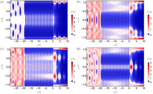
Figure S 2: Map of the LDOS as a function of the energy and the position for trivial (a,b) and topological (c,d) superconductors. Left (a,c) and right (b,d) panels correspond to on- and off-resonance cases, respectively, with values of $\mu_{\rm N_{2}}$ indicated by the dashed gray lines in Fig. 3(a) of the main text. All parameters are the same as in Fig. 3 of the main text.

On-resonance, the zero-energy LDOS for a trivial junction behaves very similar as for a topological junction, as seen in Fig. (S 2). This, however, breaks down off-resonance, where the zero-energy LDOS remain robust for the topological junction but is drastically reduced for the trivial junctions. While there are clear differences, these results point out that it might be challenging to distinguish the trivial and topological zero-energy LDOS on-resonance.

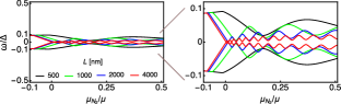
Figure S 3: Lowest energy levels of a trivial N₁N₂S with all regions being of finite length. Parameters: $L_{\rm N_{1}}=L_{\rm S}=2000$ nm, $\Delta=0.5$ meV, $\mu=0.5$ meV.

III Quasi zero-energy states in a finite length junction

In this part we show that the trivial quasi zero-energy states, discussed in the main text, remain even when the leftmost and rightmost regions have finite length, which we denote, respectively, as $L_{\rm N_{1}}$ and $L_{\rm S}$. As in the previous sections, the width of the central region is denoted $L$. We thus discretize Eq. (S 1) into a tight-binding lattice with a lattice spacing of $a=10$ nm and inspect the lowest energy level of the spectrum. This calculation is presented in Fig. S 3 for realistic parameters as a function of the chemical potential in the middle region $\mu_{\rm N_{2}}$, for different values of $L$. We observe that the lowest energy levels oscillate with $\mu_{\rm N_{2}}$ and approach zero-energy for sufficiently long middle regions. While the lowest energy states do not truly pin to zero energy, when they approach on resonance the gap between them is much smaller than one tenth of the superconducting gap. Such a small splitting would be challenging to resolve experimentally. We believe this is the critical issue when interpreting conductance data as, for all practical purposes, the trivial lowest energy states behave as a pair of Majorana bound states. We conclude this part by saying that the quasi zero-energy states presented in the main text remain robust even in finite length junctions and, thus, can be expected to occur in realistic setups.

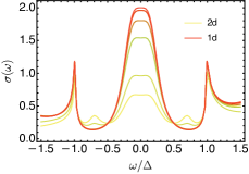
Figure S 4: Conductance of the N₁N₂S junction in the quasi-one dimensional limit. The width and doping of the central region is set on resonance with $\mu_{\text{N}2}=9.03\mu$, $k_{\text{F}}L=3\pi/2$, and $\mu_{\text{N}1}=\mu_{\text{S}}\equiv\mu=2\Delta$. We set $\lambda=0$ (two-dimensional limit), $\lambda=2,4,6,10$, and $\lambda=20$ (equivalent to one-dimensional case).

IV Quasi-one dimensional junctions

In the main text, we only considered one dimensional junctions. Most platforms for implementing Majorana bound states, even not being perfectly one-dimensional, only approach this limit after reducing the number of transverse modes contributing to transport. We now go beyond the one-dimensional limit expanding the Hamiltonian of Eq. (1) into the quasi-one dimensional limit. As a result, the momentum operator is written as $p=-i\hbar(\partial_{x}+\partial_{y})$. Considering that transport takes place along the $x$ direction, and each interface is perfectly flat in the $y$ direction, we can parametrize the transverse component of the wave vector by the angle of incidence on the leftmost normal region, $\theta=\sin^{-1}(k_{y}/k_{\text{N}1})$. For the other regions, translational invariance along the $y$ direction entails that

$$k_{\text{N}1}\sin\theta=k_{\text{N}2}\sin\theta_{\text{N}2}=k_{\text{S}}\sin\theta_{\text{S}}.$$ (S 16)

Consequently, the conductance in the normal and superconducting states, Eq. (2) and Eq. (3), respectively, must be averaged over all incident modes as

$$\langle\sigma(\omega)\rangle_{\mathbf{k}_{\parallel}}=\frac{1}{2}\int\limits^{\pi/2}_{\pi/2}\mathrm{d}\theta\cos\theta P(\theta)\sigma(\omega).$$ (S 17)

Here, $P(\theta)$ is the probability distribution for the transverse modes at the interface. We choose a Gaussian function of the form

$$P(\theta)=\exp\left(-\frac{\lambda^{2}}{2}\theta^{2}\right),$$ (S 18)

which allows us to recover the one-dimensional limit for $\lambda\rightarrow\infty$, while the planar two-dimensional case corresponds to $\lambda\rightarrow 0$. In the former case, we recover the results of the main text, while the latter case is equivalent to setting $P(\theta)=1$ in Eq. S 17.

The effect of adding extra transverse modes to the one-dimensional conductance is shown in Fig. S 4. To study the impact on the trivial zero energy states, we chose a junction on resonance featuring a quantized zero-bias conductance peak. First, the one-dimensional limit, red line in Fig. S 4, is already reproduced for $\lambda=20$. Reducing the value of the parameter $\lambda$, we approach the fully two-dimensional limit of a planar junction when $\lambda=0$ (yellow line). As we add extra modes, the magnitude of the zero-bias conductance peak is reduced, although the peak never disappears. The values in Fig. S 4 correspond, in descending order from the one-dimensional case, to $\lambda=10,6,4$, and $2$.

References

- Sato and Fujimoto [2016] M. Sato and S. Fujimoto, Majorana fermions and topology in superconductors, J. Phys. Soc. Jpn. 85, 072001 (2016).
- Sato and Ando [2017] M. Sato and Y. Ando, Topological superconductors: a review, Rep. Prog. Phys. 80, 076501 (2017).
- Aguado [2017] R. Aguado, Majorana quasiparticles in condensed matter, Riv. Nuovo Cimento 40, 523 (2017).
- Lutchyn et al. [2018] R. M. Lutchyn, E. P. Bakkers, L. P. Kouwenhoven, P. Krogstrup, C. M. Marcus, and Y. Oreg, Majorana zero modes in superconductor–semiconductor heterostructures, Nat. Rev. Mater. 3, 52 (2018).
- Zhang et al. [2019] H. Zhang, D. E. Liu, M. Wimmer, and L. P. Kouwenhoven, Next steps of quantum transport in Majorana nanowire devices, Nat. Commun. 10, 5128 (2019).
- Beenakker [2020] C. W. J. Beenakker, Search for non-Abelian Majorana braiding statistics in superconductors, SciPost Phys. Lect. Notes , 15 (2020).
- Oreg and von Oppen [2020] Y. Oreg and F. von Oppen, Majorana zero modes in networks of Cooper-pair boxes: Topologically ordered states and topological quantum computation, Annu. Rev. Condens. Matter Phys. 11, 397 (2020).
- Aguado [2020] R. Aguado, A perspective on semiconductor-based superconducting qubits, Appl. Phys. Lett. 117, 240501 (2020).
- Lutchyn et al. [2010] R. M. Lutchyn, J. D. Sau, and S. Das Sarma, Majorana fermions and a topological phase transition in semiconductor-superconductor heterostructures, Phys. Rev. Lett. 105, 077001 (2010).
- Oreg et al. [2010] Y. Oreg, G. Refael, and F. von Oppen, Helical liquids and Majorana bound states in quantum wires, Phys. Rev. Lett. 105, 177002 (2010).
- Kitaev [2001] A. Y. Kitaev, Unpaired Majorana fermions in quantum wires, Phys. Usp. 44, 131 (2001).
- Ivanov [2001] D. A. Ivanov, Non-abelian statistics of half-quantum vortices in -wave superconductors, Phys. Rev. Lett. 86, 268 (2001).
- Nayak et al. [2008] C. Nayak, S. H. Simon, A. Stern, M. Freedman, and S. Das Sarma, Non-abelian anyons and topological quantum computation, Rev. Mod. Phys. 80, 1083 (2008).
- Sarma et al. [2015] S. D. Sarma, M. Freedman, and C. Nayak, Majorana zero modes and topological quantum computation, npj Quantum Inf. 1, 15001 (2015).
- Alicea et al. [2011] J. Alicea, Y. Oreg, G. Refael, F. Von Oppen, and M. P. Fisher, Non-abelian statistics and topological quantum information processing in 1d wire networks, Nat. Phys.. 7, 412 (2011).
- Aasen et al. [2016] D. Aasen, M. Hell, R. V. Mishmash, A. Higginbotham, J. Danon, M. Leijnse, T. S. Jespersen, J. A. Folk, C. M. Marcus, K. Flensberg, and J. Alicea, Milestones toward Majorana-based quantum computing, Phys. Rev. X 6, 031016 (2016).
- Kashiwaya and Tanaka [2000a] S. Kashiwaya and Y. Tanaka, Tunnelling effects on surface bound states in unconventional superconductors, Rep. Prog. Phys. 63, 1641 (2000a).
- Bolech and Demler [2007] C. J. Bolech and E. Demler, Observing Majorana bound states in -wave superconductors using noise measurements in tunneling experiments, Phys. Rev. Lett. 98, 237002 (2007).
- Law et al. [2009] K. T. Law, P. A. Lee, and T. K. Ng, Majorana fermion induced resonant Andreev reflection, Phys. Rev. Lett. 103, 237001 (2009).
- Flensberg [2010] K. Flensberg, Tunneling characteristics of a chain of Majorana bound states, Phys. Rev. B 82, 180516 (2010).
- Lu et al. [2016] B. Lu, P. Burset, Y. Tanuma, A. A. Golubov, Y. Asano, and Y. Tanaka, Influence of the impurity scattering on charge transport in unconventional superconductor junctions, Phys. Rev. B 94, 014504 (2016).
- Burset et al. [2017] P. Burset, B. Lu, S. Tamura, and Y. Tanaka, Current fluctuations in unconventional superconductor junctions with impurity scattering, Phys. Rev. B 95, 224502 (2017).
- Mourik et al. [2012] V. Mourik, K. Zuo, S. Frolov, S. Plissard, E. Bakkers, and L. Kouwenhoven, Signatures of Majorana fermions in hybrid superconductor-semiconductor nanowire devices, Science 336, 1003 (2012).
- Higginbotham et al. [2015] A. P. Higginbotham, S. M. Albrecht, G. Kirsanskas, W. Chang, F. Kuemmeth, P. Krogstrup, T. S. J. J. Nygård, K. Flensberg, and C. M. Marcus, Parity lifetime of bound states in a proximitized semiconductor nanowire, Nat. Phys. 11, 1017 (2015).
- Deng et al. [2016] M. T. Deng, S. Vaitiekėnas, E. B. Hansen, J. Danon, M. Leijnse, K. Flensberg, J. Nygård, P. Krogstrup, and C. M. Marcus, Majorana bound state in a coupled quantum-dot hybrid-nanowire system, Science 354, 1557 (2016).
- Albrecht et al. [2016] S. M. Albrecht, A. P. Higginbotham, M. Madsen, F. Kuemmeth, T. S. Jespersen, J. Nygård, , P. Krogstrup, and C. M. Marcus, Exponential protection of zero modes in Majorana islands, Nature 531, 206 (2016).
- Zhang et al. [2017] H. Zhang, Önder Gül, S. Conesa-Boj, K. Zuo, V. Mourik, F. K. de Vries, J. van Veen, D. J. van Woerkom, M. P. Nowak, M. Wimmer, D. Car, S. Plissard, E. P. A. M. Bakkers, M. Quintero-Pérez, S. Goswami, K. Watanabe, T. Taniguchi, and L. P. Kouwenhoven, Ballistic superconductivity in semiconductor nanowires, Nat. Commun. 8, 16025 (2017).
- Suominen et al. [2017] H. J. Suominen, M. Kjaergaard, A. R. Hamilton, J. Shabani, C. J. Palmstrøm, C. M. Marcus, and F. Nichele, Zero-energy modes from coalescing Andreev states in a two-dimensional semiconductor-superconductor hybrid platform, Phys. Rev. Lett. 119, 176805 (2017).
- Nichele et al. [2017] F. Nichele, A. C. C. Drachmann, A. M. Whiticar, E. C. T. O’Farrell, H. J. Suominen, A. Fornieri, T. Wang, G. C. Gardner, C. Thomas, A. T. Hatke, P. Krogstrup, M. J. Manfra, K. Flensberg, and C. M. Marcus, Scaling of Majorana zero-bias conductance peaks, Phys. Rev. Lett. 119, 136803 (2017).
- Zhang et al. [2018] H. Zhang, C.-X. Liu, S. Gazibegovic, D. Xu, J. A. Logan, G. Wang, N. van Loo, J. D. S. Bommer, M. W. A. de Moor, D. Car, R. L. M. Op het Veld, P. J. van Veldhoven, S. Koelling, M. A. Verheijen, M. Pendharkar, D. J. Pennachio, B. Shojaei, J. S. Lee, C. J. Palmstrøm, E. P. A. M. Bakkers, S. D. Sarma, and L. P. Kouwenhoven, Retracted article: Quantized Majorana conductance, Nature 556, 74 (2018).
- Gül et al. [2018] Ö. Gül, H. Zhang, J. D. Bommer, M. W. de Moor, D. Car, S. R. Plissard, E. P. Bakkers, A. Geresdi, K. Watanabe, T. Taniguchi, et al., Ballistic Majorana nanowire devices, Nat. Nanotechnol. 13, 192 (2018).
- Kells et al. [2012] G. Kells, D. Meidan, and P. W. Brouwer, Near-zero-energy end states in topologically trivial spin-orbit coupled superconducting nanowires with a smooth confinement, Phys. Rev. B 86, 100503 (2012).
- Prada et al. [2012] E. Prada, P. San-Jose, and R. Aguado, Transport spectroscopy of nanowire junctions with Majorana fermions, Phys. Rev. B 86, 180503 (2012).
- Cayao et al. [2015] J. Cayao, E. Prada, P. San-Jose, and R. Aguado, Sns junctions in nanowires with spin-orbit coupling: Role of confinement and helicity on the subgap spectrum, Phys. Rev. B 91, 024514 (2015).
- San-José et al. [2016] P. San-José, J. Cayao, E. Prada, and R. Aguado, Majorana bound states from exceptional points in non-topological superconductors, Sci. Rep. 6, 21427 (2016).
- Liu et al. [2017] C.-X. Liu, J. D. Sau, T. D. Stanescu, and S. Das Sarma, Andreev bound states versus Majorana bound states in quantum dot-nanowire-superconductor hybrid structures: Trivial versus topological zero-bias conductance peaks, Phys. Rev. B 96, 075161 (2017).
- Ptok et al. [2017] A. Ptok, A. Kobiałka, and T. Domański, Controlling the bound states in a quantum-dot hybrid nanowire, Phys. Rev. B 96, 195430 (2017).
- Fleckenstein et al. [2018] C. Fleckenstein, F. Domínguez, N. Traverso Ziani, and B. Trauzettel, Decaying spectral oscillations in a Majorana wire with finite coherence length, Phys. Rev. B 97, 155425 (2018).
- Reeg et al. [2018] C. Reeg, O. Dmytruk, D. Chevallier, D. Loss, and J. Klinovaja, Zero-energy andreev bound states from quantum dots in proximitized rashba nanowires, Phys. Rev. B 98, 245407 (2018).
- Chen et al. [2019] J. Chen, B. D. Woods, P. Yu, M. Hocevar, D. Car, S. R. Plissard, E. P. A. M. Bakkers, T. D. Stanescu, and S. M. Frolov, Ubiquitous non-Majorana zero-bias conductance peaks in nanowire devices, Phys. Rev. Lett. 123, 107703 (2019).
- Stanescu and Tewari [2019] T. D. Stanescu and S. Tewari, Robust low-energy Andreev bound states in semiconductor-superconductor structures: Importance of partial separation of component Majorana bound states, Phys. Rev. B 100, 155429 (2019).
- Dvir et al. [2019] T. Dvir, M. Aprili, C. H. L. Quay, and H. Steinberg, Zeeman tunability of andreev bound states in van der waals tunnel barriers, Phys. Rev. Lett. 123, 217003 (2019).
- Vuik et al. [2019] A. Vuik, B. Nijholt, A. R. Akhmerov, and M. Wimmer, Reproducing topological properties with quasi-Majorana states, SciPost Phys. 7, 61 (2019).
- Avila et al. [2019] J. Avila, F. Peñaranda, E. Prada, P. San-Jose, and R. Aguado, Non-hermitian topology as a unifying framework for the Andreev versus Majorana states controversy, Commun. Phys. 2, 133 (2019).
- Pan and Das Sarma [2020] H. Pan and S. Das Sarma, Physical mechanisms for zero-bias conductance peaks in Majorana nanowires, Phys. Rev. Research 2, 013377 (2020).
- Jünger et al. [2020] C. Jünger, R. Delagrange, D. Chevallier, S. Lehmann, K. A. Dick, C. Thelander, J. Klinovaja, D. Loss, A. Baumgartner, and C. Schönenberger, Magnetic-field-independent subgap states in hybrid rashba nanowires, Phys. Rev. Lett. 125, 017701 (2020).
- Razmadze et al. [2020] D. Razmadze, E. C. T. O’Farrell, P. Krogstrup, and C. M. Marcus, Quantum dot parity effects in trivial and topological josephson junctions, Phys. Rev. Lett. 125, 116803 (2020).
- Dmytruk et al. [2020] O. Dmytruk, D. Loss, and J. Klinovaja, Pinning of Andreev bound states to zero energy in two-dimensional superconductor- semiconductor Rashba heterostructures, Phys. Rev. B 102, 245431 (2020).
- Yu et al. [2021] P. Yu, J. Chen, M. Gomanko, G. Badawy, E. P. A. M. Bakkers, K. Zuo, V. Mourik, and S. M. Frolov, Non-Majorana states yield nearly quantized conductance in proximatized nanowires, Nat. Phys. 17, 482 (2021).
- Valentini et al. [2020] M. Valentini, F. Peñaranda, A. Hofmann, M. Brauns, R. Hauschild, P. Krogstrup, P. San-Jose, E. Prada, R. Aguado, and G. Katsaros, Non-topological zero bias peaks in full-shell nanowires induced by flux tunable Andreev states, arXiv:2008.02348 (2020).
- Prada et al. [2020] E. Prada, P. San-Jose, M. W. de Moor, A. Geresdi, E. J. Lee, J. Klinovaja, D. Loss, J. Nygård, R. Aguado, and L. P. Kouwenhoven, From Andreev to Majorana bound states in hybrid superconductor–semiconductor nanowires, Nat. Rev. Phys. 2, 575 (2020).
- Ziani et al. [2020] N. T. Ziani, C. Fleckenstein, L. Vigliotti, B. Trauzettel, and M. Sassetti, From fractional solitons to Majorana fermions in a paradigmatic model of topological superconductivity, Phys. Rev. B 101, 195303 (2020).
- Moore et al. [2018] C. Moore, T. D. Stanescu, and S. Tewari, Two-terminal charge tunneling: Disentangling Majorana zero modes from partially separated Andreev bound states in semiconductor-superconductor heterostructures, Phys. Rev. B 97, 165302 (2018).
- Liu et al. [2018] C.-X. Liu, J. D. Sau, and S. Das Sarma, Distinguishing topological Majorana bound states from trivial Andreev bound states: Proposed tests through differential tunneling conductance spectroscopy, Phys. Rev. B 97, 214502 (2018).
- Hell et al. [2018] M. Hell, K. Flensberg, and M. Leijnse, Distinguishing Majorana bound states from localized Andreev bound states by interferometry, Phys. Rev. B 97, 161401 (2018).
- Ricco et al. [2019] L. S. Ricco, M. de Souza, M. S. Figueira, I. A. Shelykh, and A. C. Seridonio, Spin-dependent zero-bias peak in a hybrid nanowire-quantum dot system: Distinguishing isolated Majorana fermions from Andreev bound states, Phys. Rev. B 99, 155159 (2019).
- Yavilberg et al. [2019] K. Yavilberg, E. Ginossar, and E. Grosfeld, Differentiating Majorana from Andreev bound states in a superconducting circuit, Phys. Rev. B 100, 241408 (2019).
- Awoga et al. [2019] O. A. Awoga, J. Cayao, and A. M. Black-Schaffer, Supercurrent detection of topologically trivial zero-energy states in nanowire junctions, Phys. Rev. Lett. 123, 117001 (2019).
- Schulenborg and Flensberg [2020] J. Schulenborg and K. Flensberg, Absence of supercurrent sign reversal in a topological junction with a quantum dot, Phys. Rev. B 101, 014512 (2020).
- Zhang and Spånslätt [2020] G. Zhang and C. Spånslätt, Distinguishing between topological and quasi Majorana zero modes with a dissipative resonant level, Phys. Rev. B 102, 045111 (2020).
- Kashuba et al. [2017] O. Kashuba, B. Sothmann, P. Burset, and B. Trauzettel, Majorana STM as a perfect detector of odd-frequency superconductivity, Phys. Rev. B 95, 174516 (2017).
- Schuray et al. [2020] A. Schuray, M. Rammler, and P. Recher, Signatures of the Majorana spin in electrical transport through a Majorana nanowire, Phys. Rev. B 102, 045303 (2020).
- Grabsch et al. [2020] A. Grabsch, Y. Cheipesh, and C. W. J. Beenakker, Dynamical signatures of ground-state degeneracy to discriminate against Andreev levels in a Majorana fusion experiment, Adv. Quantum Technol. 3, 1900110 (2020).
- Pan et al. [2021] H. Pan, J. D. Sau, and S. Das Sarma, Three-terminal nonlocal conductance in majorana nanowires: Distinguishing topological and trivial in realistic systems with disorder and inhomogeneous potential, Phys. Rev. B 103, 014513 (2021).
- Liu et al. [2020] D. Liu, Z. Cao, X. Liu, H. Zhang, and D. E. Liu, Topological Kondo device for distinguishing quasi-Majorana and Majorana signatures, arXiv:2009.09996 (2020).
- Danon et al. [2020] J. Danon, A. B. Hellenes, E. B. Hansen, L. Casparis, A. P. Higginbotham, and K. Flensberg, Nonlocal conductance spectroscopy of andreev bound states: Symmetry relations and bcs charges, Phys. Rev. Lett. 124, 036801 (2020).
- Ricco et al. [2020] L. S. Ricco, J. E. Sanches, Y. Marques, M. de Souza, M. S. Figueira, I. A. Shelykh, and A. C. Seridonio, Topological isoconductance signatures in Majorana nanowires, arXiv:2004.14182 (2020).
- Thamm and Rosenow [2020] M. Thamm and B. Rosenow, Transmission amplitude through a Coulomb blockaded Majorana wire, arXiv:2010.15092 (2020).
- Chen et al. [2020] W. Chen, J. Wang, Y. Wu, J. Liu, and X. C. Xie, Non-abelian statistics of Majorana zero modes in the presence of an Andreev bound state, arXiv:2005.00735 (2020).
- Cayao and Black-Schaffer [2020] J. Cayao and A. M. Black-Schaffer, Distinguishing trivial and topological zero energy states in long nanowire junctions, arXiv:2011.10411 (2020).
- Fleckenstein et al. [2021] C. Fleckenstein, N. T. Ziani, A. Calzona, M. Sassetti, and B. Trauzettel, Formation and detection of Majorana modes in quantum spin Hall trenches, Phys. Rev. B 103, 125303 (2021).
- Ricco et al. [2021] L. S. Ricco, V. K. Kozin, A. C. Seridonio, and I. A. Shelykh, Accessing the degree of Majorana nonlocality with photons, arXiv:2105.05925 (2021).
- Tsintzis et al. [2019] A. Tsintzis, A. M. Black-Schaffer, and J. Cayao, Odd-frequency superconducting pairing in kitaev-based junctions, Phys. Rev. B 100, 115433 (2019).
- [74] See Supplemental Material at xxxx for details on how we calculate the conductance, the Green’s functions, and the LDOS for N1N2S junctions. we also present the numerical simulations for finite-size and quasi-one dimensional systems.
- Klapwijk and Ryabchun [2014] T. M. Klapwijk and S. A. Ryabchun, Direct observation of ballistic Andreev reflection, J. Exp. Theor. Phys. 119, 997 (2014).
- Klapwijk [2004] T. M. Klapwijk, Proximity effect from an Andreev perspective, J. Supercond. 17, 593 (2004).
- Blonder et al. [1982] G. E. Blonder, M. Tinkham, and T. M. Klapwijk, Transition from metallic to tunneling regimes in superconducting microconstrictions: Excess current, charge imbalance, and supercurrent conversion, Phys. Rev. B 25, 4515 (1982).
- McMillan [1968a] W. L. McMillan, Theory of superconductor-normal metal interfaces, Phys. Rev. 175, 559 (1968a).
- Furusaki and Tsukada [1991] A. Furusaki and M. Tsukada, Dc Josephson effect and Andreev reflection, Solid State Commun. 78, 299 (1991).
- Herrera et al. [2010] W. J. Herrera, P. Burset, and A. Levy Yeyati, A Green function approach to graphene–superconductor junctions with well-defined edges, J. Phys.: Condens. Matter 22, 275304 (2010).
- Burset et al. [2015] P. Burset, B. Lu, G. Tkachov, Y. Tanaka, E. M. Hankiewicz, and B. Trauzettel, Superconducting proximity effect in three-dimensional topological insulators in the presence of a magnetic field, Phys. Rev. B 92, 205424 (2015).
- Lu et al. [2015] B. Lu, P. Burset, K. Yada, and Y. Tanaka, Tunneling spectroscopy and josephson current of superconductor-ferromagnet hybrids on the surface of a 3d ti, Supercond. Sci. Technol. 28, 105001 (2015).
- Cayao and Black-Schaffer [2017] J. Cayao and A. M. Black-Schaffer, Odd-frequency superconducting pairing and subgap density of states at the edge of a two-dimensional topological insulator without magnetism, Phys. Rev. B 96, 155426 (2017).
- Lu and Tanaka [2018] B. Lu and Y. Tanaka, Study on Green’s function on topological insulator surface, Philos. Trans. R. Soc., A 376, 20150246 (2018).
- Lim et al. [2012] J. S. Lim, L. Serra, R. López, and R. Aguado, Magnetic-field instability of majorana modes in multiband semiconductor wires, Phys. Rev. B 86, 121103 (2012).
- McMillan [1968b] W. L. McMillan, Theory of superconductor—normal-metal interfaces, Phys. Rev. 175, 559 (1968b).
- Kashiwaya and Tanaka [2000b] S. Kashiwaya and Y. Tanaka, Tunnelling effects on surface bound states in unconventional superconductors, Rep. Prog. Phys. 63, 1641 (2000b).