A Broad Grid of 2D Kilonova Emission Models

Abstract

Depending upon the properties of their compact remnants and the physics included in the models, simulations of neutron star mergers can produce a broad range of ejecta properties. The characteristics of this ejecta, in turn, define the kilonova emission. To explore the effect of ejecta properties, we present a grid of 2-component 2D axisymmetric kilonova simulations that vary mass, velocity, morphology, and composition. The masses and velocities of each component vary, respectively, from 0.001 to 0.1 M_⊙ and 0.05 to 0.3$c$, covering much of the range of results from the neutron star merger literature. The set of 900 models is constrained to have a toroidal low electron fraction ($Y_{e}$) ejecta with a robust r-process composition and either a spherical or lobed high-$Y_{e}$ ejecta with two possible compositions. We simulate these models with the Monte Carlo radiative transfer code SuperNu using a full suite of lanthanide and 4th row element opacities. We examine the trends of these models with parameter variation, show how it can be used with statistical tools, and compare the model light curves and spectra to those of AT2017gfo, the electromagnetic counterpart of GW170817.

1 Introduction

The ejecta from neutron star mergers have long been believed to be a source of r-process elements (Lattimer & Schramm, 1974, 1976; Symbalisty & Schramm, 1982; Eichler et al., 1989; Davies et al., 1994). Whether or not these mergers dominate the r-process elements observed in the Galaxy depends on the amount of material ejected and the rate of mergers. The rate of mergers continues to evolve as gravitational wave observations continue (Abbott et al., 2020). Observations of GW170817 predicted a range of r-process yields depending upon the analysis of these observations and the nature of the simulations used to infer ejecta masses from the observations (Côté et al., 2018). Similarly, estimates of ejecta masses from merger calculations vary considerably depending upon both the importance of different ejecta mechanisms and the properties (e.g. masses, spins) of the binary components. This paper presents the emission from a broad range of ejecta properties to facilitate more detailed comparisons to observations of these mergers. The current variation in ejecta properties depend both upon aspects of the merger models (theoretical uncertainties) and the initial conditions of the merging binary (variations expected in nature). Until the former is constrained better, our range of models must include the range expected by both.

Simulations of the merger and post-merger environment of binary neutron stars and neutron star-black hole binaries have suggested a large number of mass ejection mechanisms, including: tidally disrupted dynamical ejecta, post-merger MHD and viscosity driven winds from the remnant system (see Shibata & Hotokezaka (2019) and references therein), shock-driven ejecta (see, for instance, Radice et al. (2018)), and cocoon outflow around the GRB jet (Gottlieb et al., 2018). The different results produced by different calculations depends, in part, upon how well the simulation technique captures these ejecta processes. The ejecta mass from merger and post-merger simulations vary over from less than 0.001 M_⊙ to nearly 0.1 M_⊙ (Dietrich et al., 2017; Bovard et al., 2017; Fujibayashi et al., 2018; Fahlman & Fernández, 2018; Radice et al., 2018; Most et al., 2019; Shibata & Hotokezaka, 2019). The masses of the binary objects have a large impact on the amount of mass ejected (Dietrich et al., 2017). The mass of the dynamical ejecta and the properties of the remnant also depend strongly on the neutron star equation of state (EOS) (Sekiguchi et al., 2015; Dietrich et al., 2017) where the remnant lifetime in turn affects the post-merger wind properties. Simulations using full general relativity and soft EOS tend to produce lower tidally-driven dynamical ejecta mass (compare, for instance, Rosswog et al. (2013) and Sekiguchi et al. (2015) - note that these two calculations use different hydrodynamic methods as well and it is possible that the hydrodynamic scheme also produces different ejecta masses).

Similarly, the simulated ejecta velocities also vary between different research groups, with average velocities lying between 0.1 and 0.6 times the speed of light, $c$ (see GW170817 estimates, for instance Kasen et al. (2017); Kawaguchi et al. (2018)). The velocity determines the degree of Doppler broadening of line features in the spectra, as well as the temperature and density at a given time. Consequently, differences on the order of $\sim 0.05-0.1c$ can have a large effect on the spectrum at a given time (see, for instance, Figure 3 of Kasen et al. (2017)).

Finally, the composition also varies considerably between different models. Ejecta with low electron fractions produces a robust heavy r-process, but many of the ejection mechanisms produce ejecta that consists of a broad range of electron fractions depending on the nature of the ejection process and the evolution of the merged object.

All of these properties (mass, velocity and composition) alter the electromagnetic signature from these mergers. At this point in time, no perfect simulation exists that captures all of the physics correctly and the variation between models reflects the assumptions in the different simulations. In addition, even if simulations converged on the properties of this ejecta for a particular progenitor binary, the range of progenitor properties (e.g. spin and masses of the merging neutron stars) will also produce a wide variety of ejecta properties. All of the ejecta properties can be simplified into a 2-component model (see Korobkin et al. (2020) and references therein) that includes one component that is very neutron-rich (primarily produced in the tidal ejecta from the initial merger) and a less neutron-rich component from disk winds, shock driven ejecta, etc. We will refer to these two components as low- and high-$Y_{e}$ respectively.

The differences in ejecta properties seen both in simulations and in the analysis of GW170817 have motivated a broad set of additional studies of both ejecta morphology, composition, masses, and velocities (Fontes et al., 2020; Tanaka et al., 2020; Kawaguchi et al., 2020; Krüger & Foucart, 2020; Korobkin et al., 2020; Barnes et al., 2020; Heinzel et al., 2020). These sets of detailed kilonova models that cover a broad range of the parameter space are essential in the analysis of kilonova observations. Here we describe a grid of 900 2D kilonova models, simulated with the Monte Carlo radiative transfer code SuperNu (Wollaeger et al., 2013; Wollaeger & van Rossum, 2014) intended for use by observers to characterize properties of observed kilonovae. These models vary mass, velocity, high-$Y_{e}$ morphology, and high-$Y_{e}$ composition. The model data used in this work are available from the LANL CTA website. This paper is organized as follows. In Section 2, we briefly review the software used to simulate the models. In Section 3, we summarize the properties and naming convention for the model outflows in which the radiative transfer is simulated. In Section 4, we verify the anticipated variation of light curves with model parameter variation, apply some example statistical tools to the model grid, and compare to the observed light curves and spectra of AT2017gfo, the electromagnetic counterpart to GW170817.

2 Codes and Numerical Methods

Our model light curves and spectra are produced with the SuperNu radiative transfer software using tabulated binned opacity (Fontes et al., 2020) from the Los Alamos suite of atomic physics codes (Fontes et al., 2015). For the composition and radioactive heating from r-process elements, we use the nucleosynthetic results from the WinNet code (Winteler et al., 2012), along with a decay network to determine the partitioning of energy among the decay products. The nucleosynthesis uses the Finite-Range Droplet Model (FRDM) (Möller et al., 1995), so the simulation results do not encompass the variability from uncertainty in nuclear mass models (Barnes et al., 2020; Zhu et al., 2021). We employ the decay product thermalization model of Barnes et al. (2016) and use grey Monte Carlo transport for the gamma-ray energy deposition (Swartz et al., 1995; Wollaeger et al., 2018).

For the opacities, we employ the binned approach demonstrated by Fontes et al. (2020). The opacity tables (including a full suite of lanthanide and 4th row elements) are over the same density and temperature grid as of Wollaeger et al. (2018), where the opacity values are computed assuming local thermodynamic equilibrium (LTE). This amounts to assuming Saha-Boltzmann statistics apply to computing ionization and excitation states (the inline SuperNu opacity calculation also assumes LTE).

In SuperNu, the radiative transfer is restricted to LTE, where the emissivity of the matter is simply the Planck function multiplied by the absorption opacity. This assumption is built into the Implicit Monte Carlo (IMC) time linearization that ultimately produces the effective scattering terms (instantaneous absorption and re-emission) Fleck & Cummings (1971). As in previous studies, the outflow is assumed homologous, where radius grows linearly with time at a velocity proportional to the radius, following the velocity grid prescription of Kasen et al. (2006). Discrete Diffusion Monte Carlo (DDMC) with opacity regrouping (Cleveland & Gentile, 2014; Wollaeger & van Rossum, 2014)) is used to optimize the radiative transfer. The DDMC Doppler shift has been given a Monte Carlo interpretation and incorporated into the opacity regrouping framework of Wollaeger & van Rossum (2014), which improves accuracy by removing one operator split in the equations (Wollaeger 2021, in prep). All SuperNu simulations are performed in 2D axisymmetric geometry, as in Korobkin et al. (2020).

3 Model Ejecta Properties

Although there are a number of ejecta processes, for our models, we simplify the ejecta into two components: a low electron fraction ejecta characteristic of the tidal ejecta that occurs during the initial merger and a high electron fraction ejecta expected from the other ejection processes (wind, shock and cocoon ejecta). Simulations of these high-$Y_{e}$ outflow mechanisms all predict roughly the same broad range of electron fractions: $Y_{e}\sim 0.2-0.5$ (see, for instance, Perego et al. (2014); Shibata & Hotokezaka (2019); Miller et al. (2019)). At this time, these different ejecta sources are difficult to distinguish. We note that three-component models may introduce a broader range of behavior in angular variation of light curves and spectra, which we have not explored in the scope of this model grid. In this section we present the model naming convention and the set of properties used to generate the 900 models in the data grid.

3.1 Model Nomenclature

We label models in the following way:

T_m<MD>_v<VD>_<S or P><N>_m<MW>_v<VW>

where T, MD, and VD are the shape, mass, and velocity of the low-$Y_{e}$ component, respectively, and S(P), N, MW, and VW, are the shape, composition, mass, and velocity of the high-$Y_{e}$ component, respectively. Masses are in units of solar mass (M_⊙) and velocities are in units of $c$. Table 1 has a summary of the properties that form the parameter space.

Table 1: Model properties per component and associated values.

Property	Values
Low-$Y_{e}$ mass	$\{0.001,0.003,0.01,0.03,0.1\}$ M⊙
High-$Y_{e}$ mass	$\{0.001,0.003,0.01,0.03,0.1\}$ M⊙
Low-$Y_{e}$ velocity	$\{0.05,0.15,0.3\}$ $c$
High-$Y_{e}$ velocity	$\{0.05,0.15,0.3\}$ $c$
Low-$Y_{e}$ morphology	Toroidal (T; Cassini oval family Korobkin et al. (2020))
High-$Y_{e}$ morphology	Spherical (S) or “Peanut” (P; Cassini oval family Korobkin et al. (2020))
Low-$Y_{e}$ composition	Robust r-process (see Table 2)
High-$Y_{e}$ composition	“High-” or “mid-” latitude wind (see options “1" and “2" in Table 2)

In the sections that follow, we use the terms "component" and "ejecta" interchangeably. We refer to the toroidal component as "low-$Y_{e}$" and the late-time non-toroidal component as "high-$Y_{e}$". We use the term "wind" only in reference to the elemental composition of the high-$Y_{e}$ component.

3.2 Mass-Velocity Grid

The grid of masses and velocities used in the models is inferred from the range of values acquired from the literature on merger, post-merger, and kilonova light curve simulations. Numerical simulations of tidal disruption produce low-$Y_{e}$ ejecta masses from $\lesssim 10^{-3}$ M_⊙ (Dietrich et al., 2017; Shibata & Hotokezaka, 2019) to $\sim 0.05$ M_⊙ for a binary neutron star system with a stiff EOS and high mass ratio (Dietrich et al., 2017). For a black hole-neutron star binary, the ejecta mass range goes up to $\sim$0.1 M_⊙ (see, for instance, Krüger & Foucart (2020)). The post-merger high-$Y_{e}$ ejecta can achieve a comparable range of values (see Table 1 of Shibata & Hotokezaka (2019)). To capture this range, our grid of mass values increase roughly by a root-decade from 0.001 to 0.1 M_⊙. We apply these five mass values to both the low- and high-$Y_{e}$ component. The values of mass are listed in the first two rows of Table 1.

Simulations of Dietrich et al. (2017) of different merger scenarios (mass ratio and EOS) also show an average low-$Y_{e}$ ejecta velocity range with error bars covering 0.1 to $0.2c$ for the low-$Y_{e}$ ejecta velocity, consistent with the 0.15 to $0.25c$ (or $\sim 0.3c$ for prompt black hole formation) range of average velocity reported by Shibata & Hotokezaka (2019). The range of possible values for the post-merger ejecta is comparable; some models of GW170817 use a faster blue component around 0.2 to $0.3c$ (Kasen et al., 2017) while others have $\sim 0.06-0.1c$ (Kawaguchi et al., 2018; Miller et al., 2019) for the fiducial model. The set of average velocities we simulate are consequently from 0.05 to 0.3$c$ for each of the two components, shown in the 3rd and 4th rows of Table 1.

3.3 Geometry

Ejecta morphology has been shown to alter the nature of the kilonova emission (Korobkin et al., 2020). Ab initio simulations of the merger produce significant tidally disrupted ejecta that is toroidally focused (see, for instance, Rosswog et al. (2013)), and here we assume the low-$Y_{e}$ dynamical ejecta is toroidal (labeled T) in morphology. Depending on EOS and the initial binary properties, simulations can produce more spherical dynamical ejecta from shocks after tidal disruption (Radice et al., 2018), but we do not consider spherical low-$Y_{e}$ ejecta. The high-$Y_{e}$ ejecta morphology is less well-constrained, but calculations of winds suggest the morphology has a lobed (axially focused or “peanut shaped”, labeled P) morphology (Miller et al., 2019; Korobkin et al., 2020). However, we include a more traditional spherical morphology (labeled S) for this late-time ejecta as well in our studies. We note that a range of high-$Y_{e}$ ejecta velocities have emerged in simulations (Shibata & Hotokezaka, 2019), and it has been argued that the smoothness of the early blue spectra of AT2017gfo indicates a fast high-$Y_{e}$ component surrounding a slower low-$Y_{e}$ component (see, for instance, Kasen et al. (2017)). The portion of our grid of models with slow low-$Y_{e}$ and fast high-$Y_{e}$ components adheres to this sort of configuration. The morphologies used for each component are listed in Table 1.

The T and P morphologies are generated using the same Cassini oval prescription as in Korobkin et al. (2020), and the S morphology is generated with the semi-analytic spherical formulae provided by Wollaeger et al. (2018). Variation over the mass-velocity grid, summarized in Section 3.2, does not change the intrinsic morphology of the ejecta. Increasing mass for a particular component uniformly scales up the density everywhere without changing the velocity coordinates, while increasing velocity stretches the morphology without changing the total mass. Both types of variation in the low-$Y_{e}$ ejecta can act to obscure the wind when the components are superimposed: increasing mass increases lanthanide partial densities, and increasing velocity covers more volume and reduces lanthanide density.

Figure 1 displays schematics of the low-$Y_{e}$ T morphology (red) combined with either the S or P-shaped winds (blue), as presented by Korobkin et al. (2020). Since each component is varied over the mass-velocity grid in Table 1, Fig. 1 does not necessarily show the correct scale of the high-$Y_{e}$ component relative to the low-$Y_{e}$ component. The model morphologies are symmetric under reflection through the (equatorial) plane bisecting the T morphology, perpendicular to the symmetry axis. Due to the stochastic nature of Monte Carlo radiative transfer simulations, equatorial reflection symmetry in the escaping flux is not strictly enforced.

Figure 1: Schematics of the two combined morphologies used in the simulation grid (Korobkin et al., 2020). All models have a toroidal (T, red) dynamical ejecta, 450 models are simulated a spherical wind (S, blue), and 450 models are simulated with a peanut-shaped wind (P, blue). Each component is varied over the mass-velocity grid in Table 1, and hence is not necessarily drawn to scale here.

3.4 Elemental Composition

The remaining ejecta property that significantly affects the emission is elemental composition. The compositions of our two components are set by the $Y_{e}$ and consist of an r-process composition for the low $Y_{e}$ ejecta (as in Even et al., 2019) and two different compositions for the high-$Y_{e}$ ejecta components, implementing a composition from an averaged $Y_{e}$ nucleosynthetic yield calculation. We use high (“wind 1”) and mid (“wind 2”) latitude compositions for the high-$Y_{e}$ component, with $Y_{e}$ values of 0.37 and 0.27 respectively (see Wollaeger et al., 2018). In Wollaeger et al. (2018), the 4th row elements were represented by a handful of surrogate elements with calculated opacities. In these calculations, we include the full suite of newly calculated 4th row elements with specific contributions enhanced to account for elements beyond the 4th row that are not included in our opacity set. These enhancements were done by comparing valence electron shells between our 4th row element and elements at higher Z (but potentially different principal quantum numbers). The elemental abundances are listed for each atomic number in Table 2; the wind abundances are plotted versus atomic number in Fig. 2 (with some of the elements labeled for convenience).

Table 2: Model abundances for the low-$Y_{e}$ (Dyn. Ej.) and high-$Y_{e}$ (Wind 1 or Wind 2) components.

El.	Z	Dyn. Ej.	Wind 1 ($Y_{e}=0.37$)	Wind 2 ($Y_{e}=0.27$)
K	19	-	3.21268e-15	6.97642e-11
Ca	20	-	1.17432e-04	2.52117e-08
Sc	21	-	2.38912e-10	4.96657e-03
Ti	22	-	3.14917e-05	3.09675e-07
V	23	-	1.49800e-04	3.64843e-07
Cr	24	-	1.26889e-01	4.73628e-02
Mn	25	-	1.81296e-03	1.19408e-06
Fe	26	5.32034e-06	8.80579e-03	2.65509e-02
Co	27	-	6.53211e-04	9.01509e-06
Ni	28	-	2.12761e-03	2.12444e-04
Cu	29	-	6.76567e-02	8.68511e-03
Zn	30	-	6.38433e-02	1.10971e-02
Ga	31	-	1.74815e-03	5.66150e-04
Ge	32	-	4.23957e-03	5.50677e-02
As	33	-	4.33796e-04	3.19672e-02
Se	34	1.01267e-01	1.92845e-01	2.84281e-01
Br	35	2.32170e-06	2.24753e-01	2.27961e-02
Kr	36	-	2.89604e-01	8.73940e-02
Zr	40	3.72218e-01	1.37605e-02	4.64549e-02
Pd	46	1.38800e-04	5.27557e-04	8.39116e-02
Te	52	3.85045e-01	5.55957e-07	2.88675e-01
La	57	5.11321e-04	-	-
Ce	58	8.65786e-04	-	-
Pr	59	8.59354e-05	-	-
Nd	60	1.49709e-03	-	-
Pm	61	5.41955e-04	-	-
Sm	62	2.03032e-03	-	-
Eu	63	1.54922e-03	-	-
Gd	64	5.12530e-03	-	-
Tb	65	3.27066e-03	-	-
Dy	66	1.39657e-02	-	-
Ho	67	3.64017e-03	-	-
Er	68	1.10523e-02	-	-
Tm	69	2.34168e-03	-	-
Yb	70	6.44273e-03	-	-
U	92	8.83764e-02	-	-

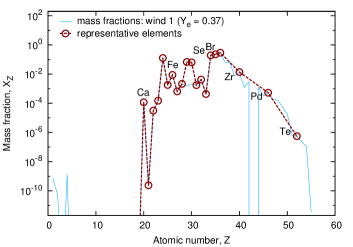
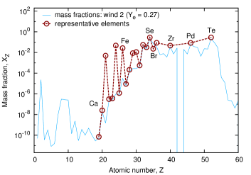
Figure 2: Representative abundances for wind 1 and wind 2 compositions (dashed red), including all of the 4th row elements from the periodic table. Deviations from original abundances account for elements with Z above 4th row: enhanced elements share similar valence electron structure with replaced elements. These compositions are applied to the high-$Y_{e}$ components of the model grid.

The low-$Y_{e}$ robust r-process dynamical ejecta composition is unchanged from Even et al. (2019) which has a simple non-lanthanide composition relative to the wind compositions. The impact of the lighter elements on the dynamical ejecta composition is small due to the effect of “lanthanide curtaining" (Barnes & Kasen, 2013; Kasen et al., 2015). Conversely, the impact of a very small fraction of lanthanides in the wind 2 composition ($\sim 10^{-7}$) is of little consequence in light curves and spectra (Even et al., 2019).

As in previous studies, the low- and high-$Y_{e}$ ejecta compositions are uniform in each component, and mixed by mass-fraction weighting in the regions of space where the components overlap. Consequently, despite wind 1 corresponding to a “high latitude” nucleosynthetic tracer, it is in fact applied to all latitudes of the high-$Y_{e}$ component morphology (as is the wind 2 composition).

4 Numerical Results

The effect of each of the model ejecta properties described in Section 3 on emission can be explored with statistics, given the size of the model grid. We present some example uses of our model grid, including basic statistics and comparison with an observation (AT2017gfo), using data in the expanded form of Table 7. Specifically, in Section 4.1 we establish the diversity in angular variation among the models, which complicates the analysis. In Section 4.2, we examine trends in means and standard deviations with variations in model properties and verify consistency with associated physics. In Section 4.3, we split the models by morphology and composition of the high-$Y_{e}$ component, and explore whether a reduced set of luminosity values can statistically distinguish the two model populations. In Section 4.4, we explore some rudimentary ways to compare the data set to AT2017gfo.

For all the models, given the geometry, the axial view is least obscured by the low-$Y_{e}$ dynamical ejecta and the edge view is most obscured, though the degree to which the low-$Y_{e}$ component is obscured depends on the relative speed of the high-$Y_{e}$ component. This is shown in Section 4.1. Since the on-axis and edge-on views represent the two extremes of light curve variation with respect to viewing angle, we restrict the data considered in Sections 4.2 and 4.3 to these views.

4.1 Viewing Angle Dependence

The degree to which the low-$Y_{e}$ ejecta obscures the blue kilonova from the high-$Y_{e}$ ejecta depends strongly on the relative speeds of the components. This dependence can be seen in the weak viewing angle variation in models with faster high-$Y_{e}$ ejecta and strong viewing angle variation in models with faster low-$Y_{e}$ ejecta. This is demonstrated in Fig. 3, which displays $g$, $r$, $z$, $J$ and $K$-band absolute AB magnitudes versus time for two models with low-$Y_{e}$ ejecta velocities at alternate extremes in the model set. Even for the lowest ratio of low-$Y_{e}$ to high-$Y_{e}$ ejecta mass, the model with fast low-$Y_{e}$ and slow high-$Y_{e}$ ejecta still produces substantial angular variation in the magnitudes (bottom panel). Alternatively, leaving all other properties unchanged, the fast high-$Y_{e}$ and slow low-$Y_{e}$ ejecta (top panel) substantially reduces the angular variation in the magnitudes. This phenomenon is the aforementioned lanthanide curtaining effect (Kasen et al., 2015), arising from the relatively high bound-bound contribution to opacity from the lanthanide abundances in the low-$Y_{e}$ component (see, for instance, Gaigalas et al. (2019); Fontes et al. (2020); Tanaka et al. (2020)). The diversity of angular variation in emission due to changes in the relative velocity of the components complicates the categorization of models based on other properties. Despite this complicating factor, in the following sections we attempt to establish expected trends collectively in the models, and determine if model morphology or composition are discernible as statistically distinct from the emission.

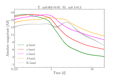
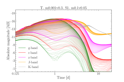
Figure 3: $g$, $r$, $z$, $J$ and $K$-band absolute AB magnitudes versus time for all viewing angles, for models with $0.001$ M_⊙ and $0.1$ M_⊙ in the low-$Y_{e}$ and high-$Y_{e}$ component, respectively. Top: low-$Y_{e}$ and high-$Y_{e}$ ejecta speed of $0.05c$ and $0.3c$, respectively. Bottom: low-$Y_{e}$ and high-$Y_{e}$ ejecta speed of $0.3c$ and $0.05c$, respectively.

4.2 Collective Data Trends

Various kilonova and supernova light curve studies have established basic trends in brightness that we expect to be reproduced in our grid of models. Specifically, we expect that increasing ejecta mass increases brightness and broadens the light curves in time (at least the bolometric luminosity), increasing the ejecta velocity increases brightness and narrows the light curves in time (shifting the peak luminosity to earlier time), and increasing the opacity decreases the brightness and broadens the light curves in time. These relationships have been encapsulated in power law relations of luminosity with respect to mass, velocity, and opacity (see, for instance, Arnett (1979); Li & Paczyński (1998); Grossman et al. (2014); Wollaeger et al. (2018)).

Here we verify that our models collectively produce the basic trends expected in two-component kilonova models with the assumed morphologies. With a large set of models uniformly spread over the space of parameters, we may perform some simple statistics to identify trends for certain parameter variations. In particular, for the axial and edge observer views, we calculate the arithmetic mean and standard deviation, per a fixed model property, of the bolometric luminosity, $g$ and $K$ bands at days one, four and eight. For luminosity, in Fig. 4 we scale by 10⁴⁰ erg/s and take the base 10 logarithm of the result in order to improve visibility of the trends,

$$\mathcal{L}=\log_{10}\left(\frac{L}{10^{40}}\right)\;\;,$$ (1)

where $\mathcal{L}$ is the scaled log luminosity that is plotted and $L$ is the original luminosity in erg/s. The day 1, 4, 8 top and side view bolometric luminosity, $g$ and $K$ band magnitudes for all 900 models are listed in the expaned form of Table 7 in Appendix A. The times are selected to sample the blue kilonova emission from the high-$Y_{e}$ component (days 1–4) and the red kilonova from the low-$Y_{e}$ component (days 4–8), and the $g$ and $K$ bands cover the relevant extremes in wavelength of the spectra.

Figure 4 has day one, four, and eight mean log luminosities versus low-$Y_{e}$ ejecta mass (left column) and low-$Y_{e}$ ejecta velocity (right column), with $\pm$1 standard deviation regions shaded about the means. The top row of panels is the axial view and the bottom row is the edge view. The mean and standard deviation are taken for the models over all other properties. Consequently, each mean or standard deviation at a given mass value is computed from 900/5=180 points of simulation data at that mass. From the left column of Fig. 4, we observe the expected trend of increasing luminosity with increasing ejecta mass. Moreover, at later times, the change in increase in luminosity per increase in mass is more pronounced, indicating that the low-$Y_{e}$ ejecta mass more strongly sets the later time luminosity. Comparing the data at day 1 for the top left and bottom left panels of Fig. 4, the luminosity at day 1 is more sensitive to the low-$Y_{e}$ ejecta mass for the edge view (bottom) than for the axial view, consistent with the low-$Y_{e}$ component having a larger effect on edge views on average. This can be seen by comparing the ratio of the mean luminosity between adjacent mass values: for the axial view the average increase in brightness is 19% and for the edge view the average increase is 36%.

As expected, the standard deviation of day 1 bolometric luminosity is not as sensitive to low-$Y_{e}$ ejecta mass as at day 4 or day 8, for either the axial or edge views. This result is consistent with the expectation that the early blue transient is not produced by the low-$Y_{e}$, lanthanide-rich component, for the parameter ranges studied. However, it is worth noting that the standard deviation of luminosities at days 1, 4, and 8 are all $\gtrsim$50% of the total luminosity at the highest mass, meaning the other ejecta properties still significantly influence the total luminosity at late time (this notion is consistent, for instance, with radiative emission from the high-$Y_{e}$ component being reprocessed into the IR by the dynamical ejecta; the high-$Y_{e}$ mass has an effect through this reprocessing).

It is more difficult to ascertain a trend in luminosity with low-$Y_{e}$ ejecta velocity, partly due to there being fewer points in the grid of models for velocity. There appears to be a weak trend at day 1, where the mean luminosity increases in the axial view as low-$Y_{e}$ ejecta velocity is increased, and decreases in the edge view as low-$Y_{e}$ ejecta velocity is increased. A physical explanation is that the higher velocity causes higher blue shift of emission from the dynamical ejecta in the observer frame, supporting a larger contribution to the total luminosity at early time (before the recession of photosphere). In contrast, for edge views, the faster low-$Y_{e}$ ejecta velocity more effectively obscure any given high-$Y_{e}$ ejecta, which acts to lower the total luminosity.

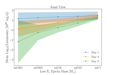
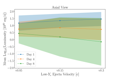
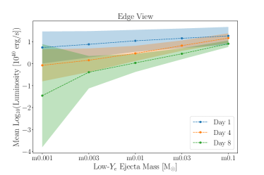
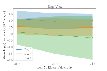
Figure 4: Mean of scaled logarithm of bolometric luminosity per low-$Y_{e}$ ejecta mass (left panels) and velocity (right panels) for axial (top panels) or edge (bottom panels) views at days 1 (blue), 4 (orange), and 8 (green). The shaded regions are $\pm$1 standard deviation around each mean (colored correspondingly). The trends follow the expected patterns: higher mass increases the luminosity at each time, and higher velocity tends to decrease the day 1 luminosity in the edge view. The variance at each value is large at day 1 across properties, but drops at day 4 and 8, indicating the low-$Y_{e}$ ejecta properties become more significant in setting the luminosity.

Figure 5 has day 1, 4, and 8 mean log luminosities versus high-$Y_{e}$ ejecta mass (left column) and high-$Y_{e}$ ejecta velocity (right column), with $\pm$1 standard deviation regions shaded about the means. Relative to Fig. 4, the bolometric luminosity in both the axial and edge views is more sensitive to high-$Y_{e}$ mass, varying by an order of magnitude from 0.001 to 0.1 M_⊙. In contrast to the variation with low-$Y_{e}$ mass, the variation in bolometric luminosity with high-$Y_{e}$ mass is greater in the axial view than in the edge view; for the axial view the average increase in brightness between adjacent high-$Y_{e}$ masses is 97%, and for the edge view it is 82%. The relative standard deviation (standard deviation over luminosity) is lowest at day 1 in the axial view for all masses, which together with the sensitivity of the mean indicates that the trend is sensitive to fewer other properties than at days 4 and 8. The high-$Y_{e}$ ejecta velocity does not appear to have a significant cumulative effect on the overall brightness, where the most significant change occurs in the edge view when going from $0.05c$ to $0.15c$; the increase of this change may again be related to the high-$Y_{e}$ component becoming less obscured by the low-$Y_{e}$ component.

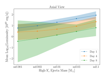
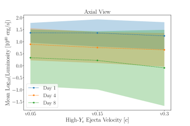
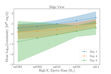
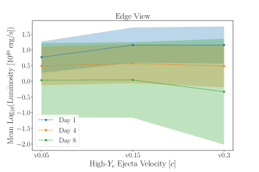
Figure 5: Mean of scaled logarithm of bolometric luminosity per high-$Y_{e}$ mass (left panels) and velocity (right panels) for axial (top panels) or edge (bottom panels) views at days 1 (blue), 4 (orange), and 8 (green). The shaded regions are $\pm$1 standard deviation around each mean (colored correspondingly). Varying high-$Y_{e}$ ejecta mass induces a significant trend in the mean luminosity at day 1; the trends for later time are consistent with reprocessing of high-$Y_{e}$ emission by the low-$Y_{e}$ ejecta.

Figure 6 has day 1, 4, and 8 axial $g$-band magnitudes versus low-$Y_{e}$ ejecta mass and velocity (top row), and high-$Y_{e}$ ejecta mass and velocity (bottom row). In contrast to the bolometric luminosity, the standard deviation in the $g$-band magnitude at day 1 is small compared to the mean magnitude. However, this is partly a result of computing standard deviation in magnitudes. As expected, we find that the variability of the $g$-band with respect to the high-$Y_{e}$ mass is more pronounced than with respect to the low-$Y_{e}$ mass. Similar to the bolometric luminosity, the mean $g$-band magnitude does not have strong trends in either low- or high-$Y_{e}$ ejecta velocities. The dependence of the $g$-band on the high-$Y_{e}$ velocity is more sensitive, but apparently non-monotonic at days 4 and 8. The drop in the mean from $0.05c$ to $0.15c$ is consistent with a reduced time scale of the blue transient, and the increase in the mean from $0.15c$ to $0.3c$ is consistent with the high-$Y_{e}$ component reprocessing more emission from the slower (or equal speed) low-$Y_{e}$ component.

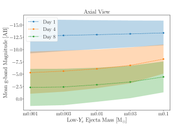
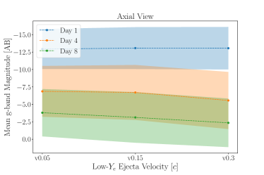
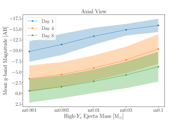
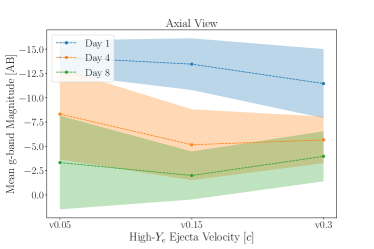
Figure 6: Mean $g$-band magnitude in axial view per low-$Y_{e}$ ejecta mass (top left) and velocity (top right), and high-$Y_{e}$ mass (bottom left) and velocity (bottom right), at days 1 (blue), 4 (orange), and 8 (green). The $g$-band magnitude trend is most apparent with increasing high-$Y_{e}$ mass, as expected. The mean $g$-band is not sensitive at day 1 to low-$Y_{e}$ ejecta mass, which is consistent with previous findings for early emission from 2-component models (Tanvir et al., 2017).

Figure 7 has the same data as Fig. 6, but for the much redder $K$-band. In contrast with the collective $g$-band results, the brightness in the $K$-band is more sensitive to the low-$Y_{e}$ ejecta mass (top left). Moreover, the change in mean magnitude between the grid mass extrema is larger for later time (comparing the day 1, 4, and 8 trend curves). This increase in sensitivity for later time is expected in the axial view, where the high-$Y_{e}$ mass plays a more dominant role in setting the brightness across bands. The magnitude of the $K$-band also trends upward for increasing high-$Y_{e}$ ejecta mass (bottom left), though there is high variability across models for each mass value.

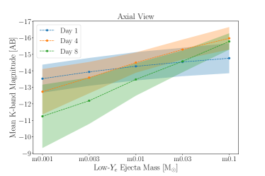
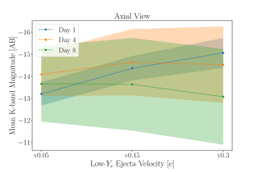
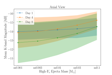
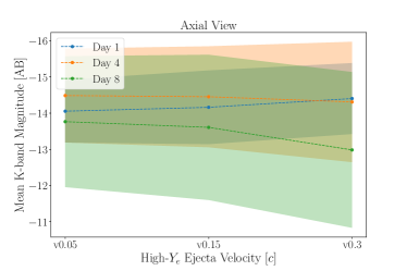
Figure 7: Mean $K$-band magnitude in axial view per low-$Y_{e}$ ejecta mass (top left) and velocity (top right), and high-$Y_{e}$ mass (bottom left) and velocity (bottom right), at days 1 (blue), 4 (orange), and 8 (green). The magnitude collectively trends upwards for both increasing low- and high-$Y_{e}$ ejecta. Moreover, the trend in low-$Y_{e}$ ejecta mass becomes significantly steeper at later time, indicating a growing impact of the low-$Y_{e}$ ejecta mass on $K$-band magnitude across models.

The collective trends of emission with respect to ejecta mass are consistent with our expectations for the behavior of 2-component kilonova models. It is more difficult to discern trends in velocity, but the weak trends that do exist readily correspond to well-established explanation (for example, lanthanide curtaining when the low-$Y_{e}$ component is faster than the high-$Y_{e}$ component). However, similar to the diversity in angular variation between models, the large standard deviations per fixed mass or velocity may obfuscate the identification of other model properties. In the following sections, we turn to the question of whether the two broadest properties, the high-$Y_{e}$ morphology and composition, when partitioned into two groups, can be statistically distinguished.

4.3 High-$Y_{e}$ Morphology and Composition Populations

We may test a null hypothesis that the data belong to the same distribution (i.e. same mean and standard deviation) when partitioned into groupings by model properties. In particular, given the differing degrees of lanthanide curtaining shown Section 4.1 and the amount of variance in trends with mass and velocity shown in Section 4.2, one may ask if broader model properties, such as high-$Y_{e}$ ejecta composition or morphology, can be statistically distinguished. Comparing these broad groupings could be performed with an analysis of variance, or similar statistical technique, to determine if the groups are distinguishable by their observable photometric properties (luminosity, magnitudes), assuming a fixed viewing angle for all models. However, with the model set, we may not be able to assume the observables are normally distributed; e.g. we may not be able to assume that the frequency of luminosity in a particular range follows a normal distribution over luminosity bins. Considering Fig. 8, we see that the distribution of axial absolute g-band magnitudes do not apparently follow normal distributions. While it may be possible to transform the observational data points to get more normal distributions, we may instead use some simple non-parametric statistical analysis to distinguish data groups.

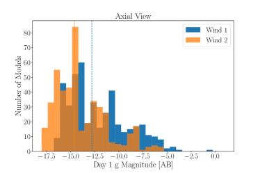
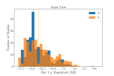
Figure 8: Histograms for fixed high-$Y_{e}$ composition (top) and morphology (bottom) of axial $g$-band absolute magnitudes over 30 uniformly spaced bins between magnitude values of -18 and 1. The histograms indicate a systematic shift between composition distributions. Medians are shown as dashed vertical lines colored by distribution.

In the following sub-sections, we explore the application of the non-parametric Mann-Whitney U test to find a subset (or “sub-vector”) of data from each model that can distinguish morphology or composition. With the sub-vector of data, we then perform a logistic regression over the models, and apply the resulting fitting parameters to fit the model data itself. With this series of calculations, we intend to demonstrate that the high-$Y_{e}$ composition of these models is easier to categorize into distinct groups than the high-$Y_{e}$ ejecta morphology.

4.3.1 Mann-Whitney U Test of Magnitudes and Luminosity

If the distributions within the partitioned groups are comparable in form, we may apply the non-parametric Mann-Whitney U test which, for two groups, tallies the number of times ($U$) that the samples in one group precede (in some ordering) the samples in another (Mann & Whitney, 1947),

$$U=mn+\frac{m(m+1)}{2}-T\;\;,$$ (2)

where $m$ and $n$ are the number of data points in each group, and $T$ is the sum of the ranks of the $m$ elements from one group in the $n+m$ ordered ranking of the total data set (the Wilcoxon statistic). The “ranks” are simply positions from sorting in the $n+m$ size list of all the data, which implies

$$\sum_{i}^{n}r_{i}+\sum_{j}^{m}s_{j}=\sum_{i}^{n}r_{i}+T\\ =\sum_{k}^{n+m}k=nm+\frac{m(m+1)}{2}+\frac{n(n+1)}{2}\;\;,$$ (3)

where $r_{i}$ and $s_{j}$ are rank subsets of $\{1,\ldots,m+n\}$ of the size $n$ and $m$ groups, respectively. The minimal rank-sum of the $r_{i}$ values is $n(n+1)/2$ (just the triangular number), which corresponds to a $U$ value of 0. An arbitrary ranking (with some $r_{i}>s_{j}$) can be formed from the $U=0$ ranking by first permuting $r_{n}=n$ with $s_{j}=n+j$, then $r_{n-1}=n-1$ with $s_{j^{\prime}}=n+j^{\prime}$ where $j^{\prime}<j$, and so forth. From this procedure, each permutation must increase the $U$ statistic by the difference of the old and new value for each $r_{i}$, since only values of $s_{j}$ will be passed over when $r_{i}$ is permuted. Consequently,

$$U=\sum_{i}^{n}(r_{i}-r_{i}^{\prime})=\sum_{i}^{n}r_{i}-\sum_{i}^{n}r_{i}^{\prime}=\sum_{i}^{n}r_{i}-\frac{n(n+1)}{2}\;\;,$$ (4)

where $r_{i}^{\prime}$ are the old ranks for $U=0$. Substituting Eq. (4) into Eq. (3) gives Eq. (2). The probability of a particular $U$ value can be found by counting the number of $n+m$ rank sequences that give $U$ from Eq. (2), and can be computed with a recurrence relation (see Mann & Whitney (1947)). We use the SciPy stats package (Virtanen et al., 2020), which has the Mann-Whitney U test as an intrinsic function.

The $U$ value can be used to test the null hypothesis that the cumulative distribution functions describing the two data sets are the same. In Fig. 8, the histograms are grouped by high-$Y_{e}$ ejecta composition (top) and high-$Y_{e}$ ejecta morphology. In these figures, it can be seen that the probability distributions are similarly shaped but may be significantly shifted in g-band brightness (especially for the grouping by composition). The distributions for the $K$ band and bolometric luminosities are also similar for these partitions of the data. Consequently, the conditions evidently suffice to use the Mann-Whitney U test over the data in the expanded form of Table 7.

Tables 3 and 4 show results of the Mann-Whitney U test for the high-$Y_{e}$ morphology and composition groups, respectively. These results include the $U$ statistic, $p$-value, and common language effect size $f$, which is the fraction of all possible pairs of data from each group that support an alternative to the null hypothesis (the null hypothesis is supported by values of $f$ close to 0.5, see McGraw & Wong (1992)). Shaded table cells indicate a $p$-value less than 0.05 (or 5%), a standard significance level for rejecting the null hypothesis. For the morphology test, the $p$-values indicate that the most significantly distinguishable cumulative distribution functions are over the $g$-band magnitudes, with axial views providing higher significance at the later days. This is consistent with the $g$-band magnitude trends shown in Fig. 9 for the on-axis view (lower panel): by day 4 there is a notable difference in the P and S morphologies for the wind 2 composition. Thus the Mann-Whitney U test verifies the apparent systematic shift between the distributions for each composition shown in Fig. 8.

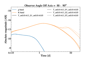
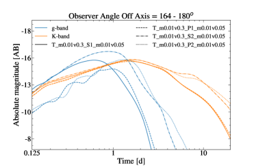
Figure 9: g (blue) and K (orange) band absolute AB magnitudes for models with $0.01$ M_⊙ mass for both high- and low-$Y_{e}$ ejecta, $0.3c$ low-$Y_{e}$ ejecta speed, and $0.05c$ high-$Y_{e}$ ejecta speed. The high-$Y_{e}$ ejecta are spherical ("S", wind 1 = solid, wind 2 = dot-dashed) and lobed ("P", wind 1 = dashed, wind 2 = dotted). The top panel is for the edge-on view and the bottom panel is for an axial view; as expected, the $g$-band is several magnitudes brighter in the axial view.

In contrast, the $p$-values for the $K$-band magnitude increase with time in both axial and edge views of the ejecta, indicating that the morphology distributions over the $K$ band become less statistically distinguishable as time progresses. The sample $K$-band magnitude curves in Fig. 9 provide evidence for this result as well, where the late time curves group by morphology and separate by composition. Moreover, only one of the six tabulated values is significant at the 5% level, while the other five do not reject the null hypothesis at this level. The bolometric luminosity likewise only has one $p$-value less than 0.05, for the day 1 edge view of the ejecta.

Table 3: Results of Mann-Whitney U test of high-$Y_{e}$ ejecta morphology (S group versus P group) per axial and edge views of $g$ band, $K$ band and bolometric luminosity $L_{\rm bol}$: $U$ statistic, $p$ value, and common language effect size $f$ at days 1, 4, and 8. $p$-values less than 5% are highlighted.

		g			K			$L_{\rm bol}$
	Day	$U$	$p$	$f$	$U$	$p$	$f$	$U$	$p$	$f$
	1	90486	$5.77\times 10^{-3}$	0.447	116240	$1.20\times 10^{-4}$	0.574	96588	0.232	0.477
Axial	4	78367	$4.39\times 10^{-9}$	0.387	107518	0.108	0.531	99476	0.649	0.491
	8	76170.5	$1.26\times 10^{-10}$	0.376	100989.0	0.947	0.499	103208	0.615	0.510
	1	83241.5	$3.86\times 10^{-6}$	0.411	107800.5	0.0928	0.532	109573	0.0328	0.541
Edge	4	94800.5	0.098	0.468	104131.5	0.460	0.514	103292	0.601	0.510
	8	109313	0.0386	0.540	97343.5	0.316	0.481	106616	0.168	0.526

The Mann-Whitney U test with partitioning in groups by composition produces more significant differences in cumulative distributions than morphology: 16 significant distribution comparisons compared to 7 for morphology at the 5% level. The $p$-value for the $g$ band is effectively zero for both axial and edge views of the ejecta (similar to the morphology test along the axial view, the $p$-value decreases towards later time). In contrast to the morphology grouping, the $K$ band at late time is a strong indicator of composition in the high-$Y_{e}$ component. The $K$-band magnitudes are close at day 1, but these magnitudes become systematically lower for the wind 1 composition; this trend is reflected in the lower $p$-values at later time. The final noteworthy difference with the morphology test is in the bolometric luminosity: for the composition test it is a significant indicator in the difference between the two populations. The difficulty of the Mann-Whitney U test in distinguishing morphology, relative to composition, is consistent with the morphology distributions being in closer alignment in Fig. 8. This pattern is noteworthy given the impact that morphology can have in brightness (Korobkin et al., 2020).

However, the Mann-Whitney U test (as presented here) does not test for differences in correlations among observables. For instance, the covariance of luminosity and $K$-band magnitude might be stronger for one morphology (composition) than the other, which would be a distinguishing factor between the morphology (composition) groups. We can calculate the Pearson correlation coefficient (Benesty et al., 2009) amongst the 9 data values per model per viewing angle ($g$ band, $K$ band, bolometric luminosity at day 1, 4, 8 for 36 comparisons per model, comparing axial-to-axial, axial-to-edge, or edge-to-edge views),

$$\varrho_{i,j}^{(P,v,w)}=\frac{\sum_{k=1}^{450}(o_{i,k}^{(P,v)}-\bar{o}_{i}^{(P,v)})(o_{j,k}^{(P,w)}-\bar{o}_{j}^{(P,w)})}{\sqrt{\sum_{k=1}^{450}(o_{i,k}^{(P,v)}-\bar{o}_{i}^{(P,v)})^{2}}\sqrt{\sum_{k=1}^{450}(o_{j,k}^{(P,w)}-\bar{o}_{j}^{(P,w)})^{2}}}\;\;,$$ (5)

where $i$ and $j$ are indices going from 1 to 9 labeling each observable, $o_{i,k}^{(P,v)}$ is the value of the observable $i$ for model with morphology P indexed at $k$, in viewing angle indexed $v$; so $\varrho_{i,j}^{(P,v,w)}\in[-1,1]$ is the Pearson correlation coefficient between $i$ and $j$ between viewing angles $v,w\in\{\text{axial},\text{edge}\}$. The maximum relative difference of correlation coefficients between morphologies is calculated as

$$\eta^{(P,S;v,w)}=\max_{i,j}\left\{\frac{|\varrho_{i,j}^{(P,v,w)}-\varrho_{i,j}^{(S,v,w)}|}{\min\{|\varrho_{i,j}^{(P,v,w)}|,|\varrho_{i,j}^{(S,v,w)}|\}}\right\}\;\;.$$ (6)

Equation (6) applies to composition if P is replaced by “wind 1” and S is replaced by “wind 2”. Using Eq. (6) for either morphology groups or composition groups, we find that the overall maximum relative difference in Pearson correlation coefficients occurs for morphology in the correlation between day 1 bolometric luminosity in the edge view and day 8 bolometric luminosity in the axial view: the correlations have the same sign ($\varrho_{i,j}^{(P,\text{axial},\text{edge})}=0.71$ and $\varrho_{i,j}^{(S,\text{axial},\text{edge})}=0.86$), but is stronger for S morphology by $\eta^{(P,S;\text{axial},\text{edge})}\sim$21%. For comparison the largest relative difference in correlation between composition groups is $\eta^{(1,2;\text{edge},\text{edge})}\sim$15%, for the correlation between day 1 $K$-band magnitude in the edge view and day 8 $g$-band magnitude also in the edge view. The Pearson correlation coefficients suggest that the impact of morphology on correlations between observables in different viewing angles per model can further distinguish the morphology groups. Given an observation is viewed at only one angle from Earth, the utility of the difference in the multi-angle correlations between the morphology groups in comparing an observation to the model grid is not readily apparent. Consequently, we focus on using the results of the Mann-Whitney U-test in forming a grid-observation comparison in the subsequent sections.

Table 4: Results of Mann-Whitney U test of high-$Y_{e}$ ejecta composition (wind 1 group versus wind 2 group) per axial and edge views of $g$ band, $K$ band and bolometric luminosity $L_{\rm bol}$: $U$ statistic, $p$ value, and common language effect size $f$ at days 1, 4, and 8. $p$-values less than 5% are highlighted.

		g			K			$L_{\rm bol}$
	Day	$U$	$p$	$f$	$U$	$p$	$f$	$U$	$p$	$f$
	1	138996.5	$3.60\times 10^{-22}$	0.686	105100	0.323	0.519	70296.5	$2.05\times 10^{-15}$	0.347
Axial	4	145124.5	$2.247\times 10^{-29}$	0.717	115642	$2.23\times 10^{-4}$	0.571	73292.5	$7.50\times 10^{-13}$	0.362
	8	158541.5	$7.04\times 10^{-49}$	0.783	123396.5	$1.34\times 10^{-8}$	0.609	72340.5	$1.19\times 10^{-13}$	0.357
	1	125232.5	$7.69\times 10^{-10}$	0.618	101830.5	0.882	0.503	82928.5	$2.62\times 10^{-6}$	0.409
Edge	4	130887	$2.94\times 10^{-14}$	0.646	114047.5	$1.03\times 10^{-3}$	0.563	77066.5	$5.55\times 10^{-10}$	0.381
	8	141209.5	$1.17\times 10^{-24}$	0.697	126966.5	$4.21\times 10^{-11}$	0.627	70454	$2.69\times 10^{-15}$	0.348

Finally, we note that we have verified the significant variables in Tables 3 and 4 with the Kolmogorov-Smirnov test, which also tests if two populations belong to the same distribution, but uses a distance metric between the partitioned distributions (Smirnov, 1948). In Section 4.3.2, we attempt to use the Mann-Whitney U test results to inform a logistic regression. The intent is to determine the effectiveness of this logistic regression in observable-based categorization of models into the morphology or composition groups.

4.3.2 Iteratively Reweighted Least Squares Categorization

The Mann-Whitney U test is a method for assessing whether two groups of data belong to one distribution over a particular parameter (the null hypothesis), but does not readily provide a way to categorize new data into a group. Consequently, for an observation or model that is not in the grid of 900, we need a different technique to determine the probability that it belongs to a particular category (for instance, of composition or morphology). One simple approach is to examine the data with the most significant $p$-values in Tables 3 or 4, and perform a multivariate logistic regression on those values. Specifically, for each model we use the data corresponding to the shaded $p$-values from those tables to perform the regression, which depends on the model property:

1. the $g$ band and day 1 $K$ band for morphology,

2. and all data except day 1 $K$ band for composition.

The fitted logistic can then be used to calculate a probability of a new observation’s inclusion in one of the groups. We attempt to fit the logistic regression parameters using an Iteratively Reweighted Least Squares (IRLS) procedure (Holland & Welsch, 1977), which is straightforward to implement using matrix manipulations available in NumPy’s linear algebra package (Harris et al., 2020). We concatenate size-$m$ sub-vectors $\vec{y}_{U}$ for each model into a 900-by-$m$ matrix $\mathbf{Y}_{U}$, where $m$ is the number of variables over which the Mann-Whitney U test distributions are significantly different. A logistic curve evaluated at each of the 900 data is

$$\vec{\mu}=\frac{1}{1+e^{-w_{0}-\mathbf{Y}_{U}\cdot\vec{w}}}\;\;,$$ (7)

where $w_{0}$ and $\vec{w}$ are a scalar and size-$m$ vector of weights. The IRLS procedure numerically solves for these weights with the following steps:

1. Calculate

   $$\mathbf{M}_{0}^{(k)}=\boldsymbol{\mu}^{(k)}\cdot(\mathbf{I}-\boldsymbol{\mu}^{(k)})\;\;,$$ (8)

   where superscript $(k)$ indicates evaluation at the $k^{\mathrm{th}}$ iteration, $\mathbf{M}_{0}^{(k)}$ is a 900x900 matrix, $\boldsymbol{\mu}^{(k)}$ is a 900x900 diagonal matrix formed from the vector in Eq. (7), and $\mathbf{I}$ is a 900x900 identity matrix.

2. Calculate

   $$\mathbf{M}_{1}^{(k)}=(\mathbf{Y}_{U}^{(k)})^{T}\cdot\mathbf{M}_{0}^{(k)}\cdot\mathbf{Y}_{U}^{(k)}\;\;,$$ (9)

   where superscript $(k)$ indicates evaluation at the $k$th iteration, $\mathbf{M}_{1}^{(k)}$ is an $m+1\times m+1$ matrix, and superscript $T$ indicates a matrix transpose.

3. Calculate

   $$\vec{M}_{2}^{(k)}=(\mathbf{Y}_{U}^{(k)})^{T}\cdot\left(\mathbf{M}_{0}^{(k)}\cdot\mathbf{Y}_{U}^{(k)}\cdot(w_{0}^{(k)},\vec{w}^{(k)})^{T}+\vec{y}-\vec{\mu}^{(k)}\right)\;\;,$$ (10)

   where $\vec{M}_{2}^{(k)}$ is a vector of size $m+1$ and $\vec{y}$ is a vector of 450 one’s and 450 zero’s, where a one indicates an S morphology or wind 2 composition.

4. Evaluate the weights for the next iteration,

   $$(w_{0}^{(k+1)},\vec{w}^{(k+1)})=(\mathbf{M}_{1}^{(k)})^{-1}\cdot\vec{M}_{2}^{(k)}\;\;,$$ (11)

   where superscript -1 indicates a matrix inverse.

The above steps are similar to a multivariate Newton iteration and maximize the log-likelihood of the logistic in Eq. (7) relative to the vector of true categorization, $\vec{y}$. The computational expense for the matrix inversion is mitigated by restricting $m$ to be the number of significant data points from the Mann-Whitney U test. In our calculation, the weights tend to be converged after five iterations. We constrain the number of parameters to four for the morphology test (three $g$ band and one $K$ band point) and eight for the composition test (three $g$ band, two $K$ band, and three bolometric luminosity points). This choice implies five and nine entries for $(w_{0},\vec{w})$ for the morphology and composition tests, respectively.

Figure 10 displays the probability of group inclusion versus model index (doubled over axial and edge views, with edge views indexed 900-1799) for the morphology test (top) and for the composition test (bottom). We have used the data set used in the regression to obtain logistic parameters, and have used this logistic fit to estimate the probability that each model is included in its own group. Despite using the parameters producing the lowest $p$-values in the Mann-Whitney U test for morphology, the logistic regression of the morphology does not fit the true categorization, and hence does not provide predictive capability for new models (within the scope of the limited data per model being used). The logistic regression for the composition groups fares somewhat better, as can be seen in the closer fit to the true composition distribution, but still suffers considerable dispersion in the probabilities (in particular, the overlap in fitted probabilities between the composition groups is large relative to the mean displacement between groups).

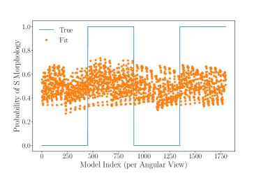
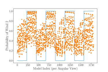
Figure 10: Fitted probabilities (orange, dotted) of the high-$Y_{e}$ component of each model having S morphology (top) or wind 2 composition (bottom) versus a model enumeration. Also shown are the true probabilities (0% or 100%) of inclusion in a group (blue, solid).

The results of the Mann-Whitney U test show the impact, collectively, of changing composition and morphology of the high-$Y_{e}$ ejecta. However, these group partitions into statistically significant differences in the distribution of observables do not provide a sufficient subset of observables to categorize new kilonova data points using the IRLS method for logistic regression. Since we have restricted our consideration to two angular views and three times of the $g$ band, $K$ band and bolometric luminosity, we may have excluded other observables that are significant indicators of morphology and composition. We have tested several different sub-vectors per categorization test, but note that the possibilities of sub-vector combinations can be expanded by using more viewing angles, broadband magnitudes, or times. Another factor that complicates the categorization of these models by composition or morphology is the diversity of the light curves over the other properties: viewing angle, high-$Y_{e}$ ejecta mass and velocity, and low-$Y_{e}$ ejecta mass and velocity. We are left to conclude that either a different fitting method over a different sub-vector of data is required, or that categorization by morphology or composition is inefficient due to the strong effects of the other model properties.

4.4 Comparison with AT2017gfo

We next compare AT2017gfo to our model data set using a logistic regression, as described in Section 4.3.2. For the sub-vector of data, we use the axial and edge luminosities at days 1, 4, and 8, given their low $p$-value from the Mann-Whitney U test in Section 4.3.1. Performing a logistic regression to fit parameter coefficients using just bolometric luminosity from the model data set, and evaluating the resulting function at the observed bolometric luminosity for AT2017gfo from Smartt et al. (2017), we find a probability estimate of $\sim$65% for a high-$Y_{e}$ component with a wind 2 composition, whereas the mean fitted probability of the data set from this regression is $\sim$46% for wind 1 models being categorized as wind 2 and $\sim$54% for wind 2 models being categorized (correctly) as wind 2. The goodness of fit is low, given the close mean probabilities, but the result suggests more closely examining models with high-$Y_{e}$ components that have wind 2 compositions.

If the probability from the Mann-Whitney U test-based IRLS logistic regression is taken to reduce the consideration to wind 2 compositions, that still leaves 450 models to consider. It may be worth reducing the number of models considered further with another metric that is simpler than the full spectra at each observed time; for instance one possible metric is an L₁ error measure of the bolometric luminosity,

$$\varepsilon_{\theta}=\frac{1}{N}\sum_{i}^{N}\frac{|L_{\theta}(t_{i})-L_{\rm obs,i}|}{L_{\rm obs,i}}\;\;,$$ (12)

where $\varepsilon_{\theta}$ is the model error at angle $\theta$ off axis, $N$ is the number of observed time points, $L_{\theta}$ is the model bolometric luminosity at $\theta$, and $L_{\rm obs,i}$ is the observed luminosity at time $t_{i}$. If we have an independent constraint that the observer angle is $\sim 18^{o}$ off-axis, we may restrict the angular views considered for Eq. (12). This particular choice of observer angle is motivated by recent estimation for GW170817, ${\theta\approx 15^{\circ}-22^{\circ}}$ (Hotokezaka et al., 2019). Table 5 has the partitioning of the number of models by the error calculated with Eq. (12) in the angular viewing bin containing $18^{o}$.

Table 5: L₁ error ranges in bolometric luminosity and corresponding number of models with wind 2 composition for the high-$Y_{e}$ component.

$\epsilon_{M,18^{o}}$	Number of Wind 2 Models
$\geq$ 1.0	329
$\geq$ 0.9, $<$ 1.0	24
$\geq$ 0.8, $<$ 0.9	21
$\geq$ 0.7, $<$ 0.8	16
$\geq$ 0.6, $<$ 0.7	16
$\geq$ 0.5, $<$ 0.6	16
$\geq$ 0.4, $<$ 0.5	20
$\geq$ 0.3, $<$ 0.4	8
$\geq$ 0.2, $<$ 0.3	0
$<$ 0.2	0

We may then examine models from a few different luminosity error groups, for instance the models and corresponding luminosity errors shown in Table 6. We have introduced an off-grid model with an average high-$Y_{e}$ ejecta velocity of 0.2$c$ for an additional comparison. The error in overall bolometric luminosity appears to systematically decrease as the ejecta velocity is increased, which would suggest that higher velocity is favored for AT2017gfo at the given viewing angle of $\sim 18^{o}$. However, in Table 6 we have constrained the other ejecta properties to specific values, so this error trend does not generally hold for all models.

Table 6: Sample models and corresponding bolometric luminosity error.

Model	$\epsilon_{M,18^{o}}$
T_m0.01v0.3_P2_m0.03v0.05	1.24
T_m0.01v0.3_P2_m0.03v0.15	0.77
T_m0.01v0.3_P2_m0.03v0.2	0.70
T_m0.01v0.3_P2_m0.03v0.3	0.45

Figure 11 has bolometric luminosity versus time for the models listed in Table 6 along with the AT2017gfo data from Smartt et al. (2017) (top left panel), and spectra versus wavelength at days 1 (top right), 3 (bottom left) and 5 (bottom right) along with VLT/X-shooter data presented by Pian et al. (2017). Despite having the lowest error in Table 6, the model with an average high-$Y_{e}$ ejecta velocity of 0.3$c$ produces a broad absorption feature between 1 and 2 $\mu$m at day 5 that is not present in the observed spectrum.

This behavior implies that a more complicated error metric may be needed to filter data, if such a step is taken before comparing spectra. This may also imply that there is some tension between the observation and the model, and that a fit should account for both consistency in spectra and in bolometric luminosity. Notably, the models with high-$Y_{e}$ ejecta velocity $>0.05c$ are all dim in the optical range relative to AT2017gfo by day 5; this is a consistent feature of our models, which warrants further investigation into both the numerical method and model assumptions.

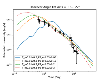
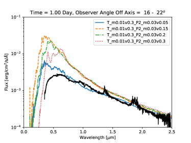
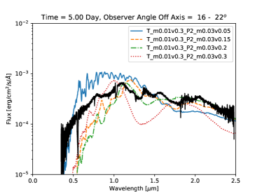
Figure 11: Luminosity versus time (top left), spectra versus wavelength at day 1 (top right), day 3 (bottom left), and day 5 (bottom right). All data are shown at an estimated observer angle of ${\theta\approx 15^{\circ}-22^{\circ}}$ (Hotokezaka et al., 2019).

5 Conclusions

We have simulated a broad grid of 900 2-component 2D axisymmetric kilonova models in order to supply a basis for model analysis and comparison to observations. Each ejecta component ranges from 0.001 to 0.1 M_⊙ in mass and 0.05 to 0.3$c$ in average ejecta speed. The model grid can support constraining the range of ejected mass from an observation or upper bound on an observation; we have indeed applied these models for the observational studies of Thakur et al. (2020), O’Connor et al. (2021) and Bruni et al. (2021). We emphasize as a caveat that the grid does not exhaust the space of possible kilonova models. For instance, this grid is not as varied in morphology as that of Korobkin et al. (2020) or as varied in composition as that of Even et al. (2019). Examples from these studies that we have not included in this grid are non-toroidal low-$Y_{e}$ ejecta and solar abundance r-process composition. Moreover, as a consequence of uncertainties in the nuclear mass models, there are uncertainties in the heating rate due to r-process (Barnes et al., 2020; Zhu et al., 2021) that we have not explored in this model grid. There has also been recent progress in non-LTE physics (Hotokezaka et al., 2021); we have not included any non-LTE treatment in the models presented here. Thus comparisons of observations to the model grid are limited by these model constraints, mass model uncertainties, and limitations in fidelity.

We have explored some example uses of the model grid in this work, including basic population statistics and comparison to the spectra of AT2017gfo. Below is a summary of this work and the corresponding results.

• The models have been simulated with multifrequency LTE radiative transfer and detailed opacities, along with detailed radioactive heating based on nucleosynthetic tracer points (Wollaeger et al., 2018) and the thermalization fraction formulation of Barnes et al. (2016). These models cover a large range of masses and velocities from the literature, but are restricted to toroidal low-$Y_{e}$ ejecta and either spherical or lobed high-$Y_{e}$ ejecta morphologies (Korobkin et al., 2020).

• Axial and edge view $g$ band, $K$ band, and bolometric luminosity values at days 1, 4 and 8 are listed in the expanded form of Table 7. We have showcased these data in an example involving the non-parametric Mann-Whitney U test for determining whether different partitions (or grouping) by properties produce statistically distinct distributions of observable properties. For this model set, the results imply that grouping by high-$Y_{e}$ composition is more effective in producing distinct distributions than grouping by high-$Y_{e}$ morphology. We emphasize that this test is possible for this model grid because there are only two morphologies and two compositions for the high-$Y_{e}$ component. A model set more exhaustive in morphology and composition would complicate this test, and generally minimize its effectiveness.

• Using observables over which the Mann-Whitney U test produces statistically distinct distributions in a logistic regression produces a low-quality fit, indicating more data (than presented in expanded Table 7) or more sophisticated techniques are needed to properly categorize observations with respect to the model data. We do find that the logistic regression performs better for the grouping by composition than for the grouping by morphology, which is consistent with the Mann-Whitney U tests.

• We have compared some of our model light curves and spectra from this grid to AT2017gfo, and find that an overly simple bolometric luminosity error estimate may filter out models that have better spectral agreement than lower-error models. The model spectra shown for high-$Y_{e}$ velocity $>0.05c$ exhibit a spectral cliff at late time, as discussed by Wollaeger et al. (2018), that is not present in the late spectrum of AT2017gfo.

The statistical study presented here can be further expanded using machine learning (ML) classification methods (see, for instance, Bishop et al. (1995); Zhang (2000)). We consider more advanced ML techniques for light curve interpolation in another work (Ristic et al., 2021). Interpolation should permit sparser initial grid requirements, which can also be achieved with Latin Hypercube sampling (see, for example, Stein (1987)). The grid we have presented here is uniform, but could be extended via Latin Hypercube sampling to account for new parameter variation. One potential impediment to Latin Hypercube sampling is the lack of an informed joint probability distribution over the model input. More observations, ab initio merger simulations, and population synthesis may help to estimate this probability distribution and enable efficient Latin Hypercube sampling.

Appendix A Magnitude Tables

Table 7: Axial / edge viewing bin for absolute AB magnitudes in g, K bands and bolometric luminosity ($L_{\rm bol}$ [$10^{40}$ erg/s]) for models with 0.001 M_⊙ dynamica ejecta and P morphology, high-latitude composition (1) wind.

	Day 1			Day 4			Day 8
Model	g	K	$L_{\rm bol}$	g	K	$L_{\rm bol}$	g	K	$L_{\rm bol}$
T_m0.001v0.05_P1_m0.001v0.05	-10.8 / -11.1	-12.2 / -11.5	2.0 / 1.6	-0.7 / -1.0	-12.1 / -11.2	0.4 / 0.2	4.0 / 4.3	-10.4 / -9.8	0.1 / 0.1
T_m0.001v0.05_P1_m0.001v0.15	-7.5 / -9.8	-12.2 / -11.3	1.1 / 1.1	0.1 / 1.0	-11.8 / -10.8	0.3 / 0.2	1.5 / 4.3	-10.3 / -9.6	0.1 / 0.1
T_m0.001v0.05_P1_m0.001v0.3	-5.9 / -5.5	-12.4 / -11.8	1.1 / 0.9	-2.5 / 2.4	-11.5 / -10.6	0.2 / 0.1	-0.8 / 4.6	-10.0 / -9.5	0.1 / 0.0
T_m0.001v0.05_P1_m0.003v0.05	-12.9 / -13.3	-12.2 / -11.6	5.1 / 5.5	-1.8 / -2.4	-12.2 / -11.6	0.5 / 0.3	3.2 / 2.7	-10.6 / -10.1	0.1 / 0.1
T_m0.001v0.05_P1_m0.003v0.15	-10.6 / -11.1	-12.2 / -11.7	2.1 / 3.1	-0.9 / 0.2	-11.9 / -11.0	0.4 / 0.2	0.6 / 3.5	-10.3 / -9.7	0.1 / 0.1
T_m0.001v0.05_P1_m0.003v0.3	-7.4 / -7.0	-12.5 / -11.7	1.5 / 1.3	-3.8 / 1.3	-11.6 / -10.6	0.3 / 0.1	-2.2 / 3.6	-10.0 / -9.5	0.1 / 0.1
T_m0.001v0.05_P1_m0.01v0.05	-13.9 / -14.2	-12.4 / -12.2	10.7 / 12.4	-5.0 / -5.5	-12.5 / -11.5	0.8 / 0.6	2.0 / 2.2	-11.2 / -11.0	0.2 / 0.1
T_m0.001v0.05_P1_m0.01v0.15	-12.8 / -13.1	-12.3 / -12.4	6.4 / 9.8	-2.0 / -0.8	-12.1 / -12.0	0.5 / 0.5	-0.4 / 2.5	-10.4 / -10.0	0.1 / 0.1
T_m0.001v0.05_P1_m0.01v0.3	-10.8 / -10.7	-12.5 / -11.7	3.6 / 6.4	-5.0 / 0.3	-11.6 / -10.7	0.4 / 0.3	-3.7 / 2.3	-10.0 / -9.5	0.1 / 0.1
T_m0.001v0.05_P1_m0.03v0.05	-14.2 / -14.5	-12.6 / -12.6	15.0 / 17.6	-8.8 / -9.3	-13.3 / -12.6	2.9 / 2.9	0.8 / 0.3	-12.0 / -12.2	0.4 / 0.4
T_m0.001v0.05_P1_m0.03v0.15	-14.7 / -15.0	-12.0 / -12.5	19.0 / 29.5	-3.3 / -2.7	-12.9 / -13.3	1.1 / 1.4	-1.3 / 1.4	-11.2 / -11.0	0.3 / 0.3
T_m0.001v0.05_P1_m0.03v0.3	-14.2 / -13.3	-12.7 / -13.1	18.8 / 22.1	-6.0 / -0.5	-12.1 / -11.4	0.9 / 0.7	-4.9 / 1.1	-10.1 / -9.6	0.2 / 0.2
T_m0.001v0.05_P1_m0.1v0.05	-14.3 / -14.6	-12.9 / -12.9	17.1 / 20.3	-12.0 / -12.2	-14.0 / -14.0	10.4 / 12.8	-3.2 / -3.8	-13.1 / -13.2	1.3 / 1.5
T_m0.001v0.05_P1_m0.1v0.15	-15.9 / -16.3	-12.6 / -13.6	55.7 / 80.7	-7.1 / -7.9	-13.7 / -12.8	3.3 / 4.8	-2.3 / 0.4	-12.7 / -12.9	0.8 / 0.9
T_m0.001v0.05_P1_m0.1v0.3	-15.7 / -15.0	-13.6 / -13.9	65.3 / 59.5	-7.1 / -2.1	-13.4 / -13.9	2.8 / 3.5	-6.0 / 0.3	-10.9 / -10.6	0.6 / 0.5
T_m0.001v0.15_P1_m0.001v0.05	-11.0 / -6.7	-13.2 / -12.3	3.4 / 0.8	2.2 / 0.3	-11.3 / -10.7	0.2 / 0.1	4.9 / 0.0	-9.8 / -9.4	0.0 / 0.0
T_m0.001v0.15_P1_m0.001v0.15	-8.4 / -8.7	-13.2 / -12.3	2.4 / 1.4	0.2 / 2.7	-11.2 / -10.6	0.2 / 0.1	1.5 / 5.3	-9.8 / -9.4	0.0 / 0.0
T_m0.001v0.15_P1_m0.001v0.3	-5.9 / -6.5	-13.3 / -12.5	1.8 / 1.2	-2.5 / 2.9	-11.0 / -10.4	0.1 / 0.1	-0.8 / 4.7	-9.4 / -9.2	0.0 / 0.0
T_m0.001v0.15_P1_m0.003v0.05	-13.4 / -8.1	-13.3 / -12.3	9.0 / 0.9	0.2 / 1.2	-11.7 / -11.3	0.3 / 0.2	4.3 / 0.6	-10.1 / -9.8	0.1 / 0.1
T_m0.001v0.15_P1_m0.003v0.15	-10.9 / -10.8	-13.4 / -12.5	4.2 / 3.2	-0.7 / 1.6	-11.4 / -10.8	0.2 / 0.2	0.6 / 3.6	-9.9 / -9.5	0.1 / 0.1
T_m0.001v0.15_P1_m0.003v0.3	-7.4 / -7.4	-13.4 / -12.5	2.3 / 1.7	-3.8 / 1.9	-11.0 / -10.4	0.2 / 0.1	-2.3 / 3.8	-9.5 / -9.2	0.0 / 0.0
T_m0.001v0.15_P1_m0.01v0.05	-14.5 / -8.8	-13.4 / -12.4	20.1 / 1.0	-4.3 / 0.9	-12.5 / -11.9	0.7 / 0.3	1.8 / 0.6	-10.9 / -10.8	0.1 / 0.1
T_m0.001v0.15_P1_m0.01v0.15	-13.0 / -13.0	-13.6 / -12.9	9.9 / 9.1	-1.9 / 0.3	-12.1 / -11.9	0.5 / 0.4	-0.3 / 2.8	-10.2 / -10.0	0.1 / 0.1
T_m0.001v0.15_P1_m0.01v0.3	-10.8 / -10.7	-13.6 / -12.7	4.8 / 6.9	-5.0 / 0.7	-11.2 / -10.7	0.3 / 0.3	-3.7 / 2.5	-9.6 / -9.3	0.1 / 0.1
T_m0.001v0.15_P1_m0.03v0.05	-14.8 / -9.2	-13.6 / -12.5	26.5 / 1.2	-9.0 / -4.0	-13.4 / -12.7	2.9 / 0.6	0.9 / 0.7	-11.9 / -12.1	0.3 / 0.3
T_m0.001v0.15_P1_m0.03v0.15	-14.9 / -14.9	-13.7 / -13.1	26.4 / 26.7	-3.3 / -2.3	-13.3 / -13.4	1.4 / 1.4	-1.2 / 2.1	-11.2 / -11.1	0.3 / 0.2
T_m0.001v0.15_P1_m0.03v0.3	-14.2 / -13.3	-13.8 / -13.6	20.2 / 22.4	-6.0 / -0.2	-12.0 / -11.6	0.8 / 0.7	-4.9 / 1.6	-10.0 / -9.7	0.2 / 0.2
T_m0.001v0.15_P1_m0.1v0.05	-14.8 / -9.4	-13.7 / -12.6	27.9 / 1.3	-12.6 / -8.7	-14.5 / -14.0	15.5 / 3.1	-3.7 / 0.6	-13.3 / -13.5	1.5 / 1.2
T_m0.001v0.15_P1_m0.1v0.15	-16.1 / -16.1	-13.9 / -13.8	69.6 / 68.4	-8.0 / -8.1	-14.2 / -13.3	5.4 / 4.9	-2.2 / 1.1	-12.9 / -13.0	0.9 / 0.9
T_m0.001v0.15_P1_m0.1v0.3	-15.7 / -14.9	-14.3 / -14.3	66.9 / 57.6	-7.1 / -1.9	-13.5 / -14.0	2.7 / 3.6	-6.0 / 0.5	-11.1 / -10.8	0.6 / 0.5
T_m0.001v0.3_P1_m0.001v0.05	-9.8 / -1.1	-13.4 / -12.6	2.2 / 0.7	1.7 / 0.3	-10.7 / -10.1	0.1 / 0.1	3.8 / 0.0	-8.4 / -7.8	0.0 / 0.0
T_m0.001v0.3_P1_m0.001v0.15	-6.9 / -5.1	-13.3 / -12.6	1.5 / 0.7	0.4 / 4.3	-10.5 / -9.8	0.1 / 0.1	1.6 / 5.6	-8.3 / -7.6	0.0 / 0.0
T_m0.001v0.3_P1_m0.001v0.3	-5.9 / -2.6	-13.2 / -12.6	1.2 / 0.8	-2.5 / 3.5	-10.5 / -9.7	0.1 / 0.1	-0.8 / 5.3	-8.1 / -7.5	0.0 / 0.0
T_m0.001v0.3_P1_m0.003v0.05	-12.8 / -1.7	-13.6 / -12.6	7.2 / 0.7	0.9 / 0.1	-11.2 / -10.9	0.1 / 0.1	5.0 / 0.0	-8.9 / -8.6	0.0 / 0.0
T_m0.001v0.3_P1_m0.003v0.15	-10.6 / -8.1	-13.5 / -12.7	3.9 / 1.1	-0.6 / 2.3	-10.7 / -10.1	0.1 / 0.1	0.8 / 5.1	-8.5 / -7.8	0.0 / 0.0
T_m0.001v0.3_P1_m0.003v0.3	-7.5 / -6.2	-13.4 / -12.6	2.1 / 1.2	-3.8 / 2.5	-10.5 / -9.8	0.1 / 0.1	-2.2 / 4.2	-8.2 / -7.6	0.0 / 0.0
T_m0.001v0.3_P1_m0.01v0.05	-14.4 / -2.9	-13.8 / -12.7	18.8 / 0.8	-2.6 / 0.4	-12.2 / -12.2	0.4 / 0.4	2.1 / 0.0	-10.2 / -10.2	0.1 / 0.1
T_m0.001v0.3_P1_m0.01v0.15	-13.0 / -10.8	-14.0 / -13.1	12.1 / 3.0	-1.8 / 2.2	-11.6 / -11.4	0.3 / 0.3	0.0 / 4.5	-9.0 / -8.7	0.1 / 0.1
T_m0.001v0.3_P1_m0.01v0.3	-10.9 / -10.4	-13.7 / -12.8	5.9 / 5.7	-5.0 / 1.5	-10.9 / -10.3	0.2 / 0.2	-3.7 / 3.1	-8.5 / -7.8	0.0 / 0.0
T_m0.001v0.3_P1_m0.03v0.05	-14.7 / -3.1	-13.9 / -12.8	25.6 / 0.9	-6.7 / 0.9	-13.5 / -13.0	2.1 / 1.0	-0.4 / 0.0	-11.5 / -11.8	0.2 / 0.2
T_m0.001v0.3_P1_m0.03v0.15	-14.9 / -13.3	-14.4 / -13.3	34.7 / 9.0	-2.9 / 0.9	-13.2 / -13.3	1.1 / 1.1	-0.9 / 2.4	-10.4 / -10.4	0.2 / 0.2
T_m0.001v0.3_P1_m0.03v0.3	-14.2 / -13.0	-14.2 / -13.8	23.9 / 19.6	-6.0 / 0.5	-12.1 / -11.5	0.8 / 0.6	-4.9 / 2.1	-9.1 / -8.5	0.2 / 0.1
T_m0.001v0.3_P1_m0.1v0.05	-14.1 / -2.1	-14.0 / -12.9	19.1 / 1.0	-11.1 / -3.6	-14.4 / -14.3	10.7 / 3.6	-2.7 / 0.0	-12.9 / -13.3	0.9 / 1.2
T_m0.001v0.3_P1_m0.1v0.15	-16.3 / -14.7	-14.6 / -13.9	93.4 / 23.3	-6.8 / -4.8	-14.6 / -14.1	6.0 / 3.7	-2.0 / 1.3	-12.5 / -12.5	0.7 / 0.7
T_m0.001v0.3_P1_m0.1v0.3	-15.7 / -14.7	-14.8 / -14.6	76.3 / 51.3	-7.1 / -1.7	-13.9 / -14.1	3.3 / 3.8	-6.0 / 0.9	-10.8 / -10.4	0.6 / 0.5

References

- Abbott et al. (2020) Abbott, R., Abbott, T. D., Abraham, S., et al. 2020, arXiv e-prints, arXiv:2010.14527
- Arnett (1979) Arnett, W. D. 1979, ApJ, 230, L37
- Barnes & Kasen (2013) Barnes, J., & Kasen, D. 2013, ApJ, 775, 18
- Barnes et al. (2016) Barnes, J., Kasen, D., Wu, M.-R., & Martínez-Pinedo, G. 2016, ApJ, 829, 110
- Barnes et al. (2020) Barnes, J., Zhu, Y. L., Lund, K. A., et al. 2020, arXiv e-prints, arXiv:2010.11182
- Benesty et al. (2009) Benesty, J., Chen, J., Huang, Y., & Cohen, I. 2009, in Noise reduction in speech processing (Springer), 1–4
- Bishop et al. (1995) Bishop, C. M., et al. 1995, Neural networks for pattern recognition (Oxford university press)
- Bovard et al. (2017) Bovard, L., Martin, D., Guercilena, F., et al. 2017, Phys. Rev. D, 96, 124005
- Bruni et al. (2021) Bruni, G., O’Connor, B., Matsumoto, T., et al. 2021, MNRAS, arXiv:2105.01440
- Cleveland & Gentile (2014) Cleveland, M. A., & Gentile, N. 2014, Journal of Computational and Theoretical Transport, 43, 6
- Côté et al. (2018) Côté, B., Fryer, C. L., Belczynski, K., et al. 2018, ApJ, 855, 99
- Davies et al. (1994) Davies, M. B., Benz, W., Piran, T., & Thielemann, F. K. 1994, ApJ, 431, 742
- Dietrich et al. (2017) Dietrich, T., Ujevic, M., Tichy, W., Bernuzzi, S., & Brügmann, B. 2017, Phys. Rev. D, 95, 024029
- Eichler et al. (1989) Eichler, D., Livio, M., Piran, T., & Schramm, D. N. 1989, Nature, 340, 126
- Even et al. (2019) Even, W., Korobkin, O., Fryer, C. L., et al. 2019, arXiv e-prints, arXiv:1904.13298
- Fahlman & Fernández (2018) Fahlman, S., & Fernández, R. 2018, ApJ, 869, L3
- Fleck & Cummings (1971) Fleck, J. A., J., & Cummings, J. D. 1971, Journal of Computational Physics, 8, 313
- Fontes et al. (2020) Fontes, C. J., Fryer, C. L., Hungerford, A. L., Wollaeger, R. T., & Korobkin, O. 2020, MNRAS, 493, 4143
- Fontes et al. (2015) Fontes, C. J., Zhang, H. L., Abdallah, J., J., et al. 2015, Journal of Physics B Atomic Molecular Physics, 48, 144014
- Fujibayashi et al. (2018) Fujibayashi, S., Kiuchi, K., Nishimura, N., Sekiguchi, Y., & Shibata, M. 2018, ApJ, 860, 64
- Gaigalas et al. (2019) Gaigalas, G., Kato, D., Rynkun, P., Radžiūtė, L., & Tanaka, M. 2019, ApJS, 240, 29
- Gottlieb et al. (2018) Gottlieb, O., Nakar, E., & Piran, T. 2018, MNRAS, 473, 576
- Grossman et al. (2014) Grossman, D., Korobkin, O., Rosswog, S., & Piran, T. 2014, MNRAS, 439, 757
- Harris et al. (2020) Harris, C. R., Millman, K. J., van der Walt, S. J., et al. 2020, Nature, 585, 357. https://doi.org/10.1038/s41586-020-2649-2
- Heinzel et al. (2020) Heinzel, J., Coughlin, M. W., Dietrich, T., et al. 2020, arXiv e-prints, arXiv:2010.10746
- Holland & Welsch (1977) Holland, P. W., & Welsch, R. E. 1977, Communications in Statistics-theory and Methods, 6, 813
- Hotokezaka et al. (2019) Hotokezaka, K., Nakar, E., Gottlieb, O., et al. 2019, Nature Astronomy, 3, 940
- Hotokezaka et al. (2021) Hotokezaka, K., Tanaka, M., Kato, D., & Gaigalas, G. 2021, arXiv e-prints, arXiv:2102.07879
- Kasen et al. (2015) Kasen, D., Fernández, R., & Metzger, B. D. 2015, MNRAS, 450, 1777
- Kasen et al. (2017) Kasen, D., Metzger, B., Barnes, J., Quataert, E., & Ramirez-Ruiz, E. 2017, Nature, 551, 80
- Kasen et al. (2006) Kasen, D., Thomas, R. C., & Nugent, P. 2006, ApJ, 651, 366
- Kawaguchi et al. (2018) Kawaguchi, K., Shibata, M., & Tanaka, M. 2018, ApJ, 865, L21
- Kawaguchi et al. (2020) —. 2020, ApJ, 889, 171
- Korobkin et al. (2020) Korobkin, O., Wollaeger, R., Fryer, C., et al. 2020, arXiv e-prints, arXiv:2004.00102
- Krüger & Foucart (2020) Krüger, C. J., & Foucart, F. 2020, Phys. Rev. D, 101, 103002
- Lattimer & Schramm (1974) Lattimer, J. M., & Schramm, D. N. 1974, ApJ, 192, L145
- Lattimer & Schramm (1976) —. 1976, ApJ, 210, 549
- Li & Paczyński (1998) Li, L.-X., & Paczyński, B. 1998, ApJ, 507, L59
- Mann & Whitney (1947) Mann, H. B., & Whitney, D. R. 1947, The annals of mathematical statistics, 50
- McGraw & Wong (1992) McGraw, K. O., & Wong, S. P. 1992, Psychological bulletin, 111, 361
- Miller et al. (2019) Miller, J. M., Ryan, B. R., Dolence, J. C., et al. 2019, Phys. Rev. D, 100, 023008
- Möller et al. (1995) Möller, P., Nix, J. R., Myers, W. D., & Swiatecki, W. J. 1995, Atomic Data and Nuclear Data Tables, 59, 185
- Most et al. (2019) Most, E. R., Papenfort, L. J., Tsokaros, A., & Rezzolla, L. 2019, ApJ, 884, 40
- O’Connor et al. (2021) O’Connor, B., Troja, E., Dichiara, S., et al. 2021, MNRAS, 502, 1279
- Perego et al. (2014) Perego, A., Rosswog, S., Cabezón, R. M., et al. 2014, MNRAS, 443, 3134
- Pian et al. (2017) Pian, E., D’Avanzo, P., Benetti, S., et al. 2017, Nature, 551, 67
- Radice et al. (2018) Radice, D., Perego, A., Hotokezaka, K., et al. 2018, ApJ, 869, L35
- Ristic et al. (2021) Ristic, M., Champion, E., O’Shaughnessy, R., et al. 2021, In prep.
- Rosswog et al. (2013) Rosswog, S., Piran, T., & Nakar, E. 2013, MNRAS, 430, 2585
- Sekiguchi et al. (2015) Sekiguchi, Y., Kiuchi, K., Kyutoku, K., & Shibata, M. 2015, Phys. Rev. D, 91, 064059
- Shibata & Hotokezaka (2019) Shibata, M., & Hotokezaka, K. 2019, Annual Review of Nuclear and Particle Science, 69, annurev
- Smartt et al. (2017) Smartt, S. J., Chen, T. W., Jerkstrand, A., et al. 2017, Nature, 551, 75
- Smirnov (1948) Smirnov, N. 1948, The annals of mathematical statistics, 19, 279
- Stein (1987) Stein, M. 1987, Technometrics, 29, 143
- Swartz et al. (1995) Swartz, D. A., Sutherland, P. G., & Harkness, R. P. 1995, ApJ, 446, 766
- Symbalisty & Schramm (1982) Symbalisty, E., & Schramm, D. N. 1982, Astrophys. Lett., 22, 143
- Tanaka et al. (2020) Tanaka, M., Kato, D., Gaigalas, G., & Kawaguchi, K. 2020, MNRAS, 496, 1369
- Tanvir et al. (2017) Tanvir, N. R., Levan, A. J., González-Fernández, C., et al. 2017, ApJ, 848, L27
- Thakur et al. (2020) Thakur, A. L., Dichiara, S., Troja, E., et al. 2020, MNRAS, 499, 3868
- Virtanen et al. (2020) Virtanen, P., Gommers, R., Oliphant, T. E., et al. 2020, Nature Methods, 17, 261
- Winteler et al. (2012) Winteler, C., Käppeli, R., Perego, A., et al. 2012, ApJ, 750, L22
- Wollaeger & van Rossum (2014) Wollaeger, R. T., & van Rossum, D. R. 2014, ApJS, 214, 28
- Wollaeger et al. (2013) Wollaeger, R. T., van Rossum, D. R., Graziani, C., et al. 2013, ApJS, 209, 36
- Wollaeger et al. (2018) Wollaeger, R. T., Korobkin, O., Fontes, C. J., et al. 2018, MNRAS, 478, 3298
- Zhang (2000) Zhang, G. P. 2000, IEEE Transactions on Systems, Man, and Cybernetics, Part C (Applications and Reviews), 30, 451
- Zhu et al. (2021) Zhu, Y. L., Lund, K. A., Barnes, J., et al. 2021, ApJ, 906, 94