Tunable High-Q Resonator by General Impedance Converter

Abstract

For the need of measurements focused in condensed matter physics and especially Bernoulli effect in superconductors we have developed an active resonator with dual operational amplifiers. A tunable high-Q resonator is performed in the schematics of the the General Impedance Converter (GIC). In the framework of frequency dependent open-loop gain of operational amplifiers, a general formula of the frequency dependence of the impedance of GIC is derived. The explicit formulas for the resonance frequency and Q-factor include as immanent parameter the crossover frequency of the operational amplifier. Voltage measurements of GIC with a lock-in amplifier perfectly agree with the derived formulas. A table reveals that electrometer operational amplifiers are the best choice to build the described resonator.

High-Q resonators with resonance frequency $f_{\mathrm{res}}$ can find many technical applications for which it is necessary to study the frequency dependence of a signal and simultaneously it is necessary this signal to be filtered by this high-Q resonator. The purpose of the present study is to represent a new possible solution of this problem in which the resonator is performed by 2 operational amplifiers (OpAmp) included in the well-known topology of the General Impedance Converter (GIC) Riordan (1967); Antoniou (1969); T. Deliyannis and Fiddler (1999); Franco (2002); Schaumann and Valkenburg (2001); Anonym (2018) drawn in Fig. 1.

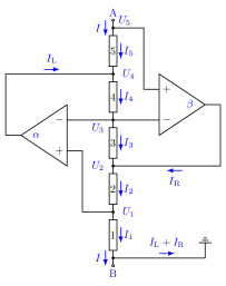
Figure 1: General Impedance Converter (GIC); the impedance $Z=U/I$ is between points A and B. $U=U_{\mathrm{A}}-U_{\mathrm{B}}$ is the voltage difference between those electrodes and $I$ is the corresponding current. The common point of the GIC (drawn intentionally upside down) is not connected with the common point of the rest of the circuit and in this sense we consider floating connection of GIC (see PCB drawing in supplementary material).

The work of the device is well described by the single pole approximation of the open-loop gain of a operational amplifier

$$G(\omega)\approx f_{c}/\mathrm{j}f,\quad\mbox{for}\quad f_{c}/G_{0}\ll f\ll f_{c},$$ (1)

where $f_{c}$ is the crossover frequency, $G_{0}\sim 10^{5}$ is the static open-loop gain, $f\equiv\omega/2\pi$ is the frequency, $\omega$ is the angular frequency, and $\mathrm{j}$ is the imaginary unit. Let us recall also the common relation between the plus $U_{+}$ and minus $U_{-}$ voltages of an OpAmp and the output one $U_{\mathrm{o}}$

$$\alpha U_{\mathrm{o}}=U_{+}-U_{-},\quad\alpha(\omega)\equiv 1/G(\omega)\approx\alpha_{0}+\tau s+\gamma s^{2},$$ (2)

where $s\equiv\mathrm{j}\omega$ is a widely used notation in electronics, $\alpha_{0}\equiv 1/G_{0}$ and the time constant $\tau=1/\omega_{c}\equiv 1/2\pi f_{c}$ is a convenient parametrization of the crossover frequency Ragazzini, Randall, and Russell (1947); Mishonov et al. (2019a); Ghausi and Laker (1991) and Ref. Franco, 2002, Eq. (6.3). The linear dependence of the reciprocal open loop gain $\alpha\approx\tau s$ is often used in many specifications of OpAmp, see for example Ref. Anonym, 2019a and cited there frequency dependent formulas for the amplification of inverting $A_{\mathrm{inv}}(\omega)=-1/[(r/R+1)\,\alpha+r/R]$ and non-inverting $A_{\mathrm{non}}(\omega)=1/[\alpha+1/(R/r+1)]$ amplifiers, where $R$ is the feedback resistance and $r$ is the gain resistance.

The schematics of the GIC analyzed in the present paper is shown in Fig. 1, where 5 impedances $Z_{1},\,Z_{2},\dots,\,Z_{5}$, voltages $U_{0},\,U_{1},\,\dots,\,U_{5}$, and currents $I_{1},\,I_{2},\dots,\,I_{5}$ are represented. For convenience $U_{5}\equiv U_{\mathrm{A}}$ and $U_{0}\equiv U_{\mathrm{B}}=0.$ The current through the impedances and voltages are related by the Ohm law

$$U_{1}-U_{0}=Z_{1}I_{1},\quad U_{2}-U_{1}=Z_{2}I_{2},$$ (3)

$$U_{3}-U_{2}=Z_{3}I_{3},\quad U_{4}-U_{3}=Z_{4}I_{4},\quad U_{5}-U_{4}=Z_{5}I_{5}.$$

We consider the input currents at the voltage inputs of the OpAmps negligible, which gives $I_{2}=I_{1}$, $I_{4}=I_{3}$ and $I_{5}=I$. The master equation Eq. (2) applied to both OpAmps gives the last equations of the system

$$U_{1}-U_{3}=\alpha U_{4},\qquad U_{5}-U_{3}=\beta U_{2}.$$ (4)

We suppose the use of a double OpAmp for which $\alpha\approx\beta$. Taking into account also the re-notation $U=U_{5}=U_{\mathrm{A}}$ and $U_{0}=U_{\mathrm{B}}=0,$ the solution of the simple system of equations

$$Z(\omega)\equiv\dfrac{U}{I} =\dfrac{Z_{5}}{1-\dfrac{(Z_{1}+Z_{2})-(Z_{3}+Z_{4})K}{(1+\beta)(Z_{1}+Z_{2})-Z_{3}K}},$$

$$K \equiv\frac{Z_{2}+(Z_{1}+Z_{2})\alpha}{Z_{3}+(Z_{3}+Z_{4})\alpha}.$$ (5)

At low frequencies $f\ll f_{c}$ and negligible $\alpha_{0}$, i.e. in the infinite open-loop gain approximation $U_{+}\approx U_{-}$ this general formula gives the well-known low frequency approximation $Z(\omega\rightarrow 0)\approx Z_{1}Z_{3}Z_{5}/Z_{2}Z_{4}.$

In the present work we analyze the case when 4 of the impedances of a GIC are resistors $Z_{1}=r_{1},$ $Z_{2}=r_{2},$ $Z_{3}=r_{3},$ $Z_{5}=r_{5}$ and only one of them is a capacitor $Z_{4}=1/\mathrm{j}\omega C_{4}$; metalized plastic thin films (polyester or polypropylene) which has dielectric loses of order $10^{-4}$. At low frequencies this approximation gives $Z=\mathrm{j}\omega L,$ where $L=C_{4}r_{1}r_{3}r_{5}/r_{2}.$ Actually simulated inductances together with D-elements Franco (2002); Inc. (2008); von Wangenheim (1996); Von Wangenheim (1997) are the main applications of GIC. In our example $r_{5}=r_{3}=1\,\mathrm{k}\Omega,$ $r_{2}=r_{1}=100\,\Omega,$ and metallized polyester film capacitor $C_{4}=10\;\mu\mathrm{F},$ which gives $L=10\,$H. This set-up was given at the 7 Experimental Physics Olympiad. Mishonov et al. (2019b)

If the GIC is sequentially connected to a load resistor $r_{l}$, as presented in Fig. 2, the sequential impedance becomes $Z_{s}\equiv Z+r_{l}$.

Figure 2: Circuit for $Z(\omega)$ measurement with Anfatec USB Lock–in 250 kHz amplifier. Anonym (2013) A sine voltage $U(t)$ from the lock-in amplifier is applied to GIC with impedance $Z(\omega)=R(\omega)+\mathrm{j}\omega L(\omega)$ and a serially connected load resistor $r_{l}$. The voltage drop $U_{r}$ on $r_{l}$ is measured by the lock-in for a range of frequencies.

For applied harmonic voltage $U(t)$ the current $I=U/Z_{s}$ and the voltage on the load resistor

$$U_{r}=\dfrac{U}{Z_{s}}r_{l}=|U_{r}|\mathrm{e}^{\mathrm{j}\varphi_{r}}=U_{r}^{\prime}+\mathrm{j}U_{r}^{\prime\prime},$$ (6)

$$\varphi_{r}(\omega)=\arctan\left(\frac{U_{r}^{\prime\prime}}{U_{r}^{\prime}}\right)\in\left(-\dfrac{\pi}{2},\,\dfrac{\pi}{2}\right),$$ (7)

$$|U_{r}(\omega)|=\sqrt{(U_{r}^{\prime})^{2}+(U_{r}^{\prime\prime})^{2}}.$$ (8)

Using a USB lock-in amplifierAnonym (2013) with $U=1\,$V and $r_{l}=10\,\Omega$ we measure the frequency dependence of the modulus $|U_{r}|$ and the phase $\varphi_{r}$ with the experimental set-up in Fig. 2. A sine voltage $U(t)$ is applied to the inductance with impedance $Z(\omega)=R(\omega)+\mathrm{j}\omega L(\omega)$ and the serially connected to it resistor $r_{l}$. The voltage drop $U_{r}$ on $r_{l}$ is measured by the lock-in amplifier for different frequencies. The experimental data and the fit according to our analytical results Eq. (Tunable High-Q Resonator by General Impedance Converter) and Eq. (8) are shown in Fig. 3.

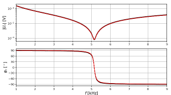
Figure 3: Voltage on the load resistor $r_{l}$ as a function of the frequency $f$. Points are experimental data, lines are calculated by our analytical results Eq. (Tunable High-Q Resonator by General Impedance Converter) and Eq. (8). Up: frequency dependence of the modulus of the voltage in log scale $|U_{r}(f)|$. The deep cusp corresponds to a high-Q resonance. Down: frequency dependence of the phase $\varphi_{r}(f)$. In a narrow frequency region $\sim f_{\mathrm{res}}/\mathcal{Q}$, close to $f_{\mathrm{res}}$, the phase decreases by 180^∘.

The fit of our theoretical formulas Eq. (Tunable High-Q Resonator by General Impedance Converter) and Eq. (8) to the experimental data for the frequency dependence modulus $|U_{r}|$ and phase $\varphi_{r}$ gives as fitting parameters of the used AD712KN Anonym (2018) $f_{c}=3.3$ MHz and $G_{0}\approx 26\times 10^{3}$.

One can see a very narrow resonance with high Q-factor $\mathcal{Q}\sim 10^{2}$ at a resonance frequency $f_{\mathrm{res}}=5.1\,$kHz. Having such an excellent fit of the experimental voltage with the analytical formula Eq. (Tunable High-Q Resonator by General Impedance Converter), one can easily calculate the real and imaginary part of the impedance of the GIC and to compare with the processed data for the impedance

$$\frac{Z(\omega)}{r_{l}} =\frac{Z^{\prime}+\mathrm{j}Z^{\prime\prime}}{r_{l}}=\frac{|Z|\mathrm{e}^{\mathrm{j}\varphi}}{r_{l}}=\left(\dfrac{U}{U_{r}}-1\right)$$ (9)

$$=\left(\dfrac{U}{|U_{r}|}\mathrm{e}^{-\mathrm{j}\varphi_{r}}\!-\!1\right)=-A_{\mathrm{inv}}(0)=\left(A_{\mathrm{non}}(0)\!-\!1\right),$$

$$Z^{\prime}(\omega) =R(\omega)=\left(\dfrac{U}{|U_{r}|}\cos(\varphi_{r})-1\right)r_{l},$$ (10)

$$Z^{\prime\prime}(\omega) =-r_{l}\dfrac{U}{|U_{r}|}\sin(\varphi_{r})=\omega L(\omega)=-\dfrac{1}{\omega C(\omega)},$$

$$L(\omega<\omega_{\mathrm{res}})>0,\qquad C(\omega>\omega_{\mathrm{res}})>0.$$

In such a way we have expressed the impedance $Z(\omega)$ of GIC by the measurable variables of modulus $|U_{r}|$ and phase $\varphi_{r}$ measured by a lock-in on a load resistor $r_{l}$ sequentially connected to GIC. Below $f_{\mathrm{res}}$ GIC is an inductance, while for frequencies higher than $f_{\mathrm{res}}$ GIC has frequency dependence as a capacitor. Qualitatively we have a parallel resonance circuit with a capacitor and inductance. It is remarkable that such a Q-factor can be easily reached even at audio frequencies. The phase changes at 180^∘ in frequency interval of only 100 Hz.

For $\omega_{\mathrm{res}}\equiv 2\pi f_{\mathrm{res}}$ and $\mathcal{Q}$ it is possible to obtain explicit analytical expressions by calculating the condition of zero conductivity $1/Z(\omega_{\mathrm{res}})=0$. Introducing

$$\Omega\equiv\omega\tau,\quad S=\mathrm{j}\Omega=\mathrm{j}\frac{f}{f_{c}}=s\tau,\quad\rho_{4}\equiv\dfrac{\tau}{C_{4}}\ll r_{3},$$

$$\epsilon_{4}\equiv\frac{\rho_{4}}{r_{3}}=\frac{\tau}{r_{3}C_{4}}\ll 1,\quad K_{1}\equiv\frac{r_{1}}{r_{1}+r_{2}},\quad K_{2}\equiv\frac{r_{2}}{r_{1}+r_{2}}$$

after some algebra from Eq. (Tunable High-Q Resonator by General Impedance Converter) the impedance

$$\frac{Z(\omega)}{r_{5}}=\frac{S^{3}+[(1+\epsilon_{4})+2a]S^{2}+[a^{2}+a+K_{1}+(1+2a)\epsilon_{4}]S+(a^{2}+a)\epsilon_{4}}{S^{3}+[(1+\epsilon_{4})+2a]S^{2}+[a^{2}+a+(1+2a)\epsilon_{4}]S+(a^{2}+a+K_{2})\epsilon_{4}},\quad a(\omega)\equiv\alpha_{0}+\gamma S^{2}.$$ (11)

The explicit formulas for the frequency dependence of the impedance of GIC Eq. (11) and Eq. (Tunable High-Q Resonator by General Impedance Converter) give the answer to every question related to the linear theory of GIC. The zeros of the denominator of Eq. (11) describe the resonances of the impedance, where the influence of $\gamma\ll 1$ is negligible and the annulation of the denominator using only the linear terms of $a$ and $\varepsilon_{2}$ gives

$$S^{3}+(1+2a+\epsilon_{4})S^{2}+(a+\epsilon_{4})S+\epsilon_{4}K_{2}=0.$$ (12)

This equation has an approximate solution at $\Omega\approx(1+\mathrm{j}/2\mathcal{Q})\,\Omega_{\mathrm{res}},\quad\Omega_{\mathrm{res}}\approx\sqrt{\epsilon_{4}K_{2}}=\tau\omega_{\mathrm{res}}\ll 1$ and

$$f_{\mathrm{res}}=\frac{\omega_{\mathrm{res}}}{2\pi}\approx\dfrac{1}{\sqrt{2\pi(1+r_{1}/r_{2})}}\sqrt{\frac{f_{c}}{r_{3}C_{4}}}\ll f_{c},$$ (13)

$$\mathcal{Q}\approx\frac{\sqrt{K_{2}\varepsilon_{4}}}{\alpha_{0}+K_{1}\varepsilon_{4}}\gg 1,$$ (14)

i.e. in order to increase Q-factor is necessary to use simultaneously high open loop gain $G_{0}=1/\alpha_{0}$ and high crossover frequency $f_{c}$. In some sense these results are derived by the Manhattan equationMishonov et al. (2019c) in action.

For optimized resonator $(\omega_{c}/G_{0})r_{3}C_{4}\sim K_{1}.$ The expression for $f_{\mathrm{res}}$ reveals that $r_{3}$ is the most convenient tunable parameter, while $r_{1}$ can be used for fine tuning. For $r_{1}\ll r_{2}$ when $K_{2}\approx 1$ we have $\Omega_{\mathrm{res}}=\sqrt{\epsilon_{4}}\ll 1,$ i.e some time dependent variable $X(t)$ obeys the oscillator equation $\mathrm{d}^{2}X(t)/\mathrm{d}t^{2}=-X(t)/r_{3}C_{4}\tau$ and the problem deserves more ingenious analysis giving the simple result $\omega_{\mathrm{res}}=1/\sqrt{\tau r_{3}C_{4}}$ directly.

For very low frequencies Eq. (11) gives Ohmic resistance

$$R_{L}\equiv Z^{\prime}(\omega\rightarrow 0)=(1+r_{1}/r_{2})r_{5}/G_{0}\ll r_{5},$$ (15)

an we have practically an ideal inductor with $L=10$ H. We wish to emphasize that our results in Eqs. (13) and (14) are based on the frequency dependent open-loop gain for the OpAmp described by Eq. (2).

The result for the Q-factor Eq. (14) deserves a detailed analysis. According to the Manhattan equationMishonov et al. (2019c) for the open-loop gain Eq. (2) $G(f)\approx(1/G_{0}+\mathrm{j}f/f_{c})^{-1}$ the crossover frequencyAnonym (2019a) is defined as a frequency for which $|G(f_{c})|=1$, that is why this frequency is also called unity gain frequency.Dostál (1993) In the same textbook by Dostal Dostál, 1993, Chap. 2 is introduced the dominant frequency

$$f_{d}\equiv f_{c}/G_{0}$$ (16)

according to which the open-loop gain in power decreases twice with respect to the zero frequency $|G(f_{d})|^{2}=G_{0}^{2}/2.$ Using these notions Eq. (14) reads

$$\mathcal{Q}=\dfrac{\dfrac{f_{\mathrm{res}}}{f_{d}}}{1+\dfrac{r_{1}}{r_{2}}\left(\dfrac{f_{\mathrm{res}}}{f_{c}}\right)\left(\dfrac{f_{\mathrm{res}}}{f_{d}}\right)}\gg 1.$$ (17)

For special case of $r_{1}=r_{2}$ introducing $x\equiv f_{\mathrm{res}}/f_{c}$ the Q-factor writes $\mathcal{Q}(x)=x/(G_{0}^{-1}+x^{2})$. This function has a maximum $\mathcal{Q}_{\mathrm{max}}=\sqrt{G_{0}}/2$ at $x_{\mathrm{max}}=1/\sqrt{G_{0}}$, i.e. at $f_{\mathrm{max}}=f_{c}/\sqrt{G_{0}}=\sqrt{f_{d}f_{c}}$ is the resonance frequency at $\mathcal{Q}_{\mathrm{max}}$. Usually the unity gain frequency $f_{c}$ is so high that the second term in the denominator gives only several percent contribution and with acceptable for the choice of OpAmps, we can use the approximation

$$\mathcal{Q}\approx f_{\mathrm{res}}/f_{d}\gg 1.$$ (18)

In other words the dominant frequency $f_{d}=f_{c}/G_{0}$ is the most important parameter for the choice of OpAmp used for the described resonator. For an ideal OpAmp with $f_{c}=\infty$ and $G_{0}=\infty$ this resonance cannot be described; it is necessary to precise also that $f_{d}=f_{c}/G_{0}=0$ which gives ideal $\mathcal{Q}=\infty$. In Table 1 the parameters for the frequently used OpAmps are given.

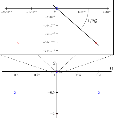
Figure 6: Poles ($\star$) and zeros ($\circ$) of the GIC impedance $Z(\omega)$ in the complex plane of the frequency $\Omega\equiv\omega\tau$, where $\omega\equiv-\mathrm{i}s=\omega^{\prime}+\mathrm{i}\omega^{\prime\prime}$, all of them in the lower semi-plane. The zero $\omega_{0}\approx-\mathrm{i}R_{L}/L$ describes current decay $\propto\mathrm{e}^{-(R_{L}/L)t}$ of DC current through the simulated inductance. The two pole resonances $\omega_{\pm}\approx\pm\omega_{\mathrm{res}}-\mathrm{i}\omega_{\mathrm{res}}/2\mathcal{Q}$ describe time decay of the voltage amplitude $\propto\mathrm{e}^{-(\omega_{\mathrm{res}}/2\mathcal{Q})t}\mathrm{e}^{-\mathrm{i}\omega_{\mathrm{res}}t}$ and energy of oscillations $\propto\mathrm{e}^{-(\omega_{\mathrm{res}}/\mathcal{Q})t}$. The other zeros and pole are irrelevant for the low frequency behavior of the GIC. For real frequencies and sinusoidal voltages $U(t)=\Re(U_{\omega}\mathrm{e}^{-\mathrm{i}\mathrm{\omega}t})$ and currents $I(t)=\Re(I_{\omega}\mathrm{e}^{-\mathrm{i}\mathrm{\omega}t})$ the impedance $Z(\omega)\equiv U_{\omega}/I_{\omega}$ and the conductivity $\sigma(\omega)\equiv 1/Z(\omega)=I_{\omega}/U_{\omega}$ describe linear responses of the system with respect to small perturbations. For damping modes of a stable system $Z(\omega)$ and $1/Z(\omega)$ are analytical functions in the upper $\omega$ semi-plane and one can calculate the Fourier transforms to time domain $Z(t)=\int_{-\infty}^{+\infty}\mathrm{e}^{-\mathrm{i}\omega t}Z(\omega)(\mathrm{d}\omega/2\pi)=\theta(t)Z(t)$ and $\sigma(t)=\int_{-\infty}^{+\infty}\mathrm{e}^{-\mathrm{i}\omega t}\sigma(\omega)(\mathrm{d}\omega/2\pi)=\theta(t)\sigma(t)$. The Heaviside $\theta$-function describes the causality principle: $I(t)=\int_{0}^{\infty}\sigma(t^{\prime})U(t-t^{\prime})\mathrm{d}t^{\prime}$ and analogously $U(t)=\int_{-\infty}^{t}Z(t-t^{\prime})I(t^{\prime})\mathrm{d}t^{\prime}$. For more details related to Kramers and Kronig causality principles, see for example the section on generalized susceptibility from the textbook on statistical physics by Landau and Lifshitz. The amplitude of the plane wave in optics is $\propto\exp[\mathrm{i}(\mathbf{k}\cdot\mathbf{r}-\omega t)]$, where the relation $\mathrm{j}=-\mathrm{i}$ comes from. Let $\zeta>0$ is a positive variable, $s=\zeta$ and $\omega=\mathrm{i}\zeta$ is purely imaginary. In this case $Z(\omega=\mathrm{i}\zeta)=\int_{0}^{+\infty}\mathrm{e}^{-\zeta t}Z(t)\,\mathrm{d}t.$ If the impedance is a passive system in thermal equilibrium with temperature $T$ the Matsubara frequency is discrete $\zeta_{n}=2n\pi k_{\mathrm{B}}T/\hbar$, where $n=0,1,2,\dots.$

OpAmp	$f_{c}$ [MHz]	$G_{0}$ {$10^{6}$}	$f_{d}$ [Hz]	Reference
ADA4530	2	14	0.14	Anonym, 2017, Table 1, Fig. 55
AD549	1	1.0	1.0	Anonym, 2015a, Fig 8, Fig. 14
AD8544	1	0.5	2.0	Anonym, 2011, Table 1, Fig. 18
TL072	5	1.0	5.0	Anonym, 2020, p. 15, Fig. 6-8
AD712	4	0.4	10	Anonym, 2018, Table 1, Fig. 11
ADA4610	9.3	0.1	93	Anonym, 2019b, Table 2, Fig. 26
LTC6269	300	0.25	1 200	Anonym, 2014, Table 2, G21
ADA4898	100	0.05	2 000	Anonym, 2015b, Table 1, Fig. 19
ADA4817	400	0.0014	286$\times 10^{3}$	Anonym, 2019a, Table 2, Fig. 31

Table 1: According to the approximate Eq. (18)

the best Q-factor is reached by the lowest dominant frequencies $f_{d}$. The table reveals that electrometer OpAmps are the best choice to build the described resonators. On the other hand low-noise and high frequency amplifiers are unsuitable for this purpose. The estimation according to Eq. 17 and further analysis show that one can expect with ADA4530Anonym (2017) one can reach $\mathcal{Q}>1000$ and with the other electrometer AD549Anonym (2015a) $\mathcal{Q}\approx 500$ both at kHz range.

Usually finite frequency of the crossover frequency $f_{c}$ is considered as some non-ideality of an OpAmp but the purpose of the present paper is to demonstrate that this inequality can be used for something useful, to design and create tunable high-Q resonators for various applications.Muñoz, Berga, and Escrivá (2005); Muñoz et al. (2006); Montero et al. (2007); Borodjieva and Manukova-Marinova (2004) In other words, the novelty of the proposed scheme is based on the immanent property of the operational amplifiers – the finite crossover frequency $f_{c}$. Recently we have also developed a method for fast and accurate measurement of the crossover frequency of operational amplifiers.Mishonov et al. (2021) All these studies are part of a creation of instrument for measurements focused in condensed matter physics and especially Bernoulli effect in superconductors.Mishonov and Varonov (2021) In conclusion in order to reach $\mathcal{Q}>100$ it is recommended to use a contemporary electrometer OpAmp.

Toshiro Mifune and Alberto Barone wish to thank to Hassan Chamati for the hospitality in the Georgi Nadjakov Institute of Solid State Physics and creative atmosphere during this long time endeavor. Albert Varonov would like to acknowledge the support by the Joint Institute for Nuclear Research, Dubna, Russian Federation - THEME 01-3-1137-2019/2023 and Grant No D01-378/18.12.2020 of the Ministry of Education and Science of Bulgaria.

Appendix A Supplementary Experimental Data

A.1 Signal + Noise Input and Output from Oscilloscope Output

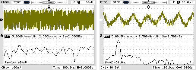
Figure 4: Two screenshots from digital oscilloscope (Rigol DS1052E) screen of a typical application of a resonance filter performed by GIC. Left: A sum of white noise (1 V peak to peak) and small sinusoidal signal (50 mV peak to peak, $f_{\mathrm{res}}=5.05$ kHz), signal to noise ratio 1/20, is applied from a signal generator (Rigol DG1022) to sequentially connected load resistor (100 k$\Omega$) and GIC, this is the input signal of the filter. Right: Voltage on the GIC in this voltage divider, this is the output signal of the filter. The small sinusoidal signal is recovered by suppressing the noise outside of the resonance. In technical applications of measurement of small signals Q-factor of the resonator multiplies the dynamic diapason of the lock-in voltmeter. The output signal passes through a voltage repeater with TL072 operational amplifier because of the giant modulus impedance of the GIC in the resonance, much larger than the input impedance of the oscilloscope (1 M$\Omega$), see Fig. 3. Both oscilloscope screens are vertically divided in half: the upper part represents the time dependence of the voltages, while the lower part gives the spectral density of the signals mathematically calculated by the oscilloscope from the voltage signal shown in the upper part. On the left one can see approximately constant spectral density of white noise, the small sine signal cannot be seen even in the spectral density. On the right the resonance maximum becomes visible due to suppressing of the non-resonance frequencies. The scale of all figures is different and it can be easily seen that the recovered sinusoidal signal has the same amplitude as the input sinusoidal signal. This recovered sine signal dominates the output signal spectral density.

A.2 PCB Layout

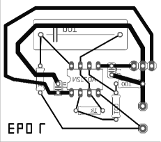
Figure 5: Printed Circuit Board (PCB) of the the resonator performed by GIC; topology is depicted in Fig. 1. One can see the place for the big metal-layer capacitor $C=10\,\mu\mathrm{F}$; $Z_{4}=1/\mathrm{j}\omega C$, the places of the small resistors $Z_{2}=Z_{1}=100\,\Omega$, and the places of the big resistors $Z_{5}=Z_{3}=1\,\mathrm{k}\Omega$. Not shown in Fig. 1: places for small ceramic capacitors capacitors which are connected to the voltage supply batteries are close to the 8 pin locus for the operational amplifier. The 3 pins on the right are for voltage supply $V_{\mathrm{S-}}$, floating (not connected) common point, and voltage supply $V_{\mathrm{S+}}$, This set-up was given to the participants of the 7-th Experimental Physics Olympiad, see Ref. [12]. At low frequency below 50 Hz high students measured that it is an artificial inductance $L=10$ H. The new idea of the present study is to demonstrate that this GIC has inherent high-Q resonance which is perfectly described by the single pole approximation Eq. (1) of the frequency dependent open-loop gain. The novelty of our result is that this opportunity has never been used to create a tunable high-Q resonator. Our motivation is to create a new set-up for measurement of small signals in the physics of superconductivity. The two pins on the lower right part of figure are the 2 electrodes of the GIC used to connect it in a circuit.

Appendix B Poles and Zeros in the Complex Frequency Plane

Appendix C Alternative Enumeration of the GIC Impedances

In Fig. 1 the impedances are numbered as floors of a building from the ground upwards. However in Fig. 8.45 of Ref. Inc., 2008 and the numbering is opposite, as rows of a matrix from up to down, i.e. enumeration (1, 2, 3, 4, 5) from the used above notation should be substituted by (5, 4, 3, 2, 1). In the enumeration used by Zumbahlen Inc. (2008) our main results Eq. (Tunable High-Q Resonator by General Impedance Converter) reads

$$Z(\omega)=\dfrac{Z_{1}}{1-\dfrac{Z_{3}Z_{5}-Z_{2}Z_{4}}{Z_{3}Z_{5}+Z_{4}Z_{5}\left[\alpha Z_{2}+\beta Z_{3}+\alpha\beta(Z_{2}+Z_{3})\right]}}\;.$$ (19)

Additionally, here we wish to point out that Fig. 8.46 and Figs. 8.47 A, B and C of Ref. Inc., 2008 have erroneous topology, which is corrected in Fig. 8.48.

Concerning the terminology in Ref. Inc., 2008 the notion: “general impedance converter” is used, while some authors recommend “generalized impedance converter”. We do not express an opinion but just a comparison “general relativity” or “generalized relativity” has to be called the Einstein theory for the geometrodymanics.

References

Riordan (1967)R. Riordan, “Simulated
inductors using differential amplifiers,” El. Lett. 3, 50–51 (1967).
Antoniou (1969)A. Antoniou, “Realisation
of gyrators using operational amplifiers, and their use in rc-active-network
synthesis,” Proc. IEE 116, 1838–1850 (1969).
T. Deliyannis and Fiddler (1999)Y. S. T. Deliyannis and J. K. Fiddler, Continuous-Time Active
Filter Design (CRC-Press, New York, 1999).
Franco (2002)S. Franco, “Design with operational amplifiers
and analog integrated circuits,” (McGraw Hill, New York, 2002) Chap. 4, 3rd ed.
Schaumann and Valkenburg (2001)R. Schaumann and M. E. V. Valkenburg, “Design of analog filters,” (Oxford University Press, New
York, 2001) Chap. 4.
Ragazzini, Randall, and Russell (1947)J. R. Ragazzini, R. H. Randall, and F. A. Russell, “Analysis of
problems in dynamics by electronic circuits,” Proc.
IRE 35, 444–452
(1947).
Mishonov et al. (2019a)T. M. Mishonov, V. I. Danchev, E. G. Petkov,
V. N. Gourev, I. M. Dimitrova, N. S. Serafimov, A. A. Stefanov, and A. M. Varonov, “Master equation for operational amplifiers:
stability of negative differential converters, crossover frequency and
pass-bandwidth,” J. Phys. Comm. 3, 035004 (2019a).
Inc. (2008)A. D. Inc., “Linear circuit design handbook,” (Newnes/Elsevier, New York, 2008) Chap. 8, pp. 8.68–8.69, GIC Figs. 8.45 and 8.46.
von Wangenheim (1996)L. von
Wangenheim, “Modification
of the classical GIC structure and its application to RC-oscillators,” Electronics Letters 32, 6–8(2) (1996).
Von Wangenheim (1997)L. Von Wangenheim, “Pspice
tunes oscillator circuits,” EDN 42, 121–122 (1997).
Mishonov et al. (2019b)T. M. Mishonov, R. Popeski-Dimovski, L. Velkoska, I. M. Dimitrova, V. N. Gourev, A. P. Petkov,
E. G. Petkov, and A. M. Varonov, “The Day of the Inductance.
Problem of the 7-th Experimental Physics Olympiad, Skopje, 7 December
2019,” (2019b), arXiv:1912.07368 [physics.ed-ph]
.
Mishonov et al. (2019c)T. M. Mishonov, A. A. Stefanov, E. G. Petkov, I. M. Dimitrova, V. I. Danchev, V. N. Gourev,
and A. M. Varonov, “Manhattan equation for the
operational amplifier,” in 10th Jubilee International Conference of the Balkan
Physical Union, Vol. 2075 (AIP Publishing, 2019) p. 160002.
Dostál (1993)J. Dostál, “Operational amplifiers,” (Butterworth-Heinemann, New
York, 1993) Chap. 2 Operational
Amplifier Parameters, 2nd ed., sec. 2.1 Linear Parameters and Linear Model.
Muñoz, Berga, and Escrivá (2005)D. R. Muñoz, S. C. Berga, and C. R. Escrivá, “Current loop generated from
a generalized impedance converter: A new sensor signal conditioning
circuit,” Rev. Sci. Instr. 76, 066103 (2005).
Muñoz et al. (2006)D. R. Muñoz, J. S. Moreno,
S. C. Berga, E. C. Montero, C. R. Escrivá, and A. E. N. Antón, “Temperature compensation of wheatstone bridge
magnetoresistive sensors based on generalized impedance converter with input
reference current,” Rev. Sci. Instr. 77, 105102 (2006).
Montero et al. (2007)E. C. Montero, D. R. Muñoz,
J. S. Moreno, J. F. Barrio, and A. S. Mustelier, “Signal conditioning for differential
temperature measurement with thermistors using a generalized impedance
converter,” Rev. Sci. Instr. 78, 086114 (2007).
Mishonov et al. (2021)T. M. Mishonov, E. G. Petkov, I. M. Dimitrova, N. S. Serafimov, and A. M. Varonov, “Probability
distribution function of crossover frequency of operational amplifiers,” Measurement 179, 109509 (2021), arXiv:1802.09342v3 [eess.SP]
.