Effective GUP-modified Raychaudhuri equation and black hole singularity: four models

Abstract

The classical Raychaudhuri equation predicts the formation of conjugate points for a congruence of geodesics, in a finite proper time. This in conjunction with the Hawking-Penrose singularity theorems predicts the incompleteness of geodesics and thereby the singular nature of practically all spacetimes. We compute the generic corrections to the Raychaudhuri equation in the interior of a Schwarzschild black hole, arising from modifications to the algebra inspired by the generalized uncertainty principle (GUP) theories. Then we study four specific models of GUP, compute their effective dynamics as well as their expansion and its rate of change using the Raychaudhuri equation. We show that the modification from GUP in two of these models, where such modifications are dependent of the configuration variables, lead to finite Kretchmann scalar, expansion and its rate, hence implying the resolution of the singularity. However, the other two models for which the modifications depend on the momenta still retain their singularities even in the effective regime.

1 Introduction

As is well-known, most reasonable classical spacetimes are singular, in the sense of geodesic incompleteness, as predicted by the celebrated Hawking-Penrose singularity theorems. The essential ingredient behind the formulation of these theorems, namely the Raychaudhuri equation, predicts the convergence of geodesics in a finite proper time, and this leads directly to their incompleteness Raychaudhuri:1953yv ; Penrose:1964wq ; Hawking:1969sw .

The above singularity being classical however, it is expected that it will be resolved by a consistent theory of Quantum Gravity (QG). This is particularly true for black holes and in particular the Schwarzschild model. While classically a physical singularity exists in the interior of this black hole, the hope is that quantum gravity effects will lead to its resolution. This issue has been studied in various approaches to quantum gravity, in particular, in loop quantum gravity (LQG), which is a nonperturbative canonical approach to quantization of gravity Thiemann:2007pyv . Within LQG, both the interior and the full spacetime of Schwarzschild and also lower dimensional black holes have been studied (see. e.g., Bojowald:2004af ; Ashtekar:2005qt ; Bojowald:2005cb ; Bohmer:2007wi ; Corichi:2015xia ; Barrau:2018rts ; Alesci:2019pbs ; Aruga:2019dwq ; Bodendorfer:2019cyv ; Brahma:2014gca ; Campiglia:2007pb ; Chiou:2008nm ; Corichi:2015vsa ; Cortez:2017alh ; Gambini:2008dy ; Gambini:2009ie ; Gambini:2011mw ; Gambini:2013ooa ; Gambini:2020nsf ; Husain:2004yz ; Kelly:2020uwj ; Thiemann:1992jj ; Campiglia:2007pr ; Gambini:2009vp ; Rastgoo:2013isa ; Corichi:2016nkp ; Morales-Tecotl:2018ugi ; Blanchette:2020kkk and the references within). If one only considers the interior, then the metric mimics the metric of the Kantowski-Sachs (KS) cosmological model and one is dealing with a minisuperspace model, meaning a gravitational system with finite dimensional classical phase space. Within LQG, this model is usually quantized using polymer quantization Ashtekar:2002sn ; Corichi:2007tf ; Morales-Tecotl:2016ijb ; Tecotl:2015cya ; Flores-Gonzalez:2013zuk by first symmetry reducing the model at the classical level and then applying the quantization procedure (although other works, such as Alesci:2019pbs , exist in which reduction is done after quantization). The polymer quantization introduces a (set of) parameter(s) into the theory called the polymer scale. These parameters set minimal scales of the model which determine the onset of quantum gravitational effects. These works show a general effective way of avoiding the singularity.

There has been a phenomenological approach to studying certain problems in QG, via the so-called Generalized Uncertainty Principle (GUP). Various approaches to QG, black hole physics etc. predict the existence of a minimum measurable length and/or a maximum measurable angular momentum. For example, examining string theory and its related scattering amplitudes beyond the Planck scale strongly suggests such a length Amati:1988tn ; Gross:1987ar as does some other approaches to quantum gravity. This leads to a deformation of the standard Heisenberg commutation relation, which in turn induces correction terms to practically all quantum mechanical Hamiltonians. This leads to QG effects in a range of systems from the laboratory based to the astrophysical, including potentially measurable ones in the context of black holes and cosmology AMELINO_CAMELIA_2002 ; Amelino_Camelia_2001 ; Cort_s_2005 ; Pikovski_2012 ; Marin:2013pga ; Bawaj_2015 ; Amelino_Camelia_2013 ; Hossenfelder_2013 ; Amati:1988tn ; Kempf:1994su ; Maggiore:1993rv ; Maggiore_1994 ; Adler_2001 ; Das_2008 ; Nozari_2008 ; Alonso_Serrano_2018 ; Myung_2007 ; Bargue_o_2015 ; Gangopadhyay_2018 ; Ali_2014 ; Ali_2015 ; Das_2011 ; Sprenger_2011 ; Ali_2011 ; Rovelli:1994ge ; Garay:1994en ; Scardigli:1999jh ; AmelinoCamelia:2008qg ; Bosso:2018ckz ; Bosso:2017hoq ; Bosso:2018uus ; Bosso:2019ljf ; Casadio_2020 ; Bosso:2020aqm ; Todorinov_2019 ; Bosso_2020 ; Bosso_2021 ; Bonder:2017ckx ; Das_2020 ; das2021bounds ; Garcia-Chung:2020zyq ; Stargen_2019 ; das2021test . However, GUP in the context of the Raychaudhuri equation, its deformations and the subsequent implications for singularity resolution, to the best of our knowledge has not been studied extensively. We investigate this further in this article. The role of GUP in the interior of black holes has been investigated recently in Bosso:2020ztk ; preparation1 . Corrections to the Raychaudhuri equation from other sources and its implications to singularity resolution in quantum gravity and cosmology was studied in Das_2014 ; Das_2015 ; Burger_2018 ; Das_2019 .

In this paper, we investigate the modified dynamics of the interior of the Schwarzschild black hole using Ashtekar-Barbero variables but using modified algebra inspired by GUP. We consider a generic class of deformations of the Poisson algebra assuming that such modification are the phenomenological result of similar modifications at the quantum level. Using this modified algebra, we derive the dynamics of the generic equations of motion of the interior and based on that find the expansion $\theta$ and its rate of change $\frac{d\theta}{d\tau}$ (with $\tau$ being the proper time) using the Raychaudhuri equation. Then, we discuss the general conditions under which $\theta$ and $\frac{d\theta}{d\tau}$ remain finite everywhere in the interior. The finiteness of these quantities implies that no caustic points for congruence of geodesics, and consequently no singularity, exists. We then choose four specific subcases of this generic class of models in which the modifications are either linear or quadratic in configuration variable or the momenta. We derive the detailed dynamics of each case as well as the explicit expression for $\theta$ and $\frac{d\theta}{d\tau}$ in relevant cases. We then show that in two of the four cases in which the modifications depend on the configuration variables, the Kretchmann scalar, $\theta$ and $\frac{d\theta}{d\tau}$ remain finite everywhere in the interior, which implies the resolution of the singularity. However, in the two other cases in which the modifications depend on the momenta, the Kretchmann scalar diverges even in the effective regime and the singularity persists. Hence, for the latter two cases we do not compute $\theta$ and $\frac{d\theta}{d\tau}$.

The structure of this manuscript is as follows. In Sec. 2 we review the dynamics of the interior of the Schwarzschild black hole in the classical regime using the Ashtekar-Barbero variables. In Sec. 3, we briefly discuss the Raychaudhuri equation, its significance and its classical expression and behavior for the interior of the Schwarzschild black hole. In Sec. 4, we introduce the generic class of the GUP modifications we are considering and derive the generic form of $\theta$ and $\frac{d\theta}{d\tau}$ for this class using the generic dynamics of the interior and the Raychaudhuri equation. We also discuss the conditions under which $\theta$ and $\frac{d\theta}{d\tau}$ remain finite. In Sec. 5 we consider four specific models within the generic class mentioned. These are the most common models used in GUP. We analyze both the dynamics and the behavior of $\theta$ and $\frac{d\theta}{d\tau}$ in these models and show that in two of them the singularity is resolved while in the other two it persists even in the effective regime. Finally, in Sec. 6 we summarize our work and conclude and also discuss some possible future directions.

2 Classical Schwarzschild interior and its dynamics

It is well-known that by switching the coordinates $t$ and $r$ in the metric of the Schwarzschild black hole

$$ds^{2}=-\left(1-\frac{2GM}{r}\right)dt^{2}+\left(1-\frac{2GM}{r}\right)^{-1}dr^{2}+r^{2}d\Omega^{2},$$ (1)

one can obtain the metric of the interior as

$$ds^{2}=-\left(\frac{2GM}{t}-1\right)^{-1}dt^{2}+\left(\frac{2GM}{t}-1\right)dr^{2}+t^{2}d\Omega^{2},$$ (2)

where now $t$ is the Schwarzschild interior time that takes values in the range $t\in(0,2GM)$. In this form, $t$ is the radius of the 2-spheres inside the black hole. The above metric is a special case of a Kantowski-Sachs (KS) cosmological spacetime that is given by the metric Collins:1977fg

$$ds_{KS}^{2}=-N(T)^{2}dT^{2}+g_{xx}(T)dx^{2}+g_{\theta\theta}(T)d\theta^{2}+g_{\phi\phi}(T)d\phi^{2}.$$ (3)

Note that $x$ here can be a rescaling of the coordinate $r$ in (2), and $T$ is the generic KS time corresponding to the choice of he lapse $N(T)$. The KS spacetime is a spatially homogeneous but anisotropic model. Its spatial hypersurfaces have topology $\mathbb{R}\times\mathbb{S}^{2}$, and its symmetry group is the KS isometry group $\mathbb{R}\times SO(3)$.

We are interested in expressing the model in terms of the Ashtekar-Barbero connection $A_{a}^{i}$ and its conjugate, the desitized triad $\tilde{E}_{i}^{a}$. It turns out that due to the symmetry of the model, $A_{a}^{i},\,\tilde{E}_{i}^{a}$ adapted to this spacetime can be written as Ashtekar:2005qt

$$A_{a}^{i}\tau_{i}dx^{a}= \frac{c}{L_{0}}\tau_{3}dx+b\tau_{2}d\theta-b\tau_{1}\sin\theta d\phi+\tau_{3}\cos\theta d\phi,$$ (4)

$$\tilde{E}_{i}^{a}\tau_{i}\partial_{a}= p_{c}\tau_{3}\sin\theta\partial_{x}+\frac{p_{b}}{L_{0}}\tau_{2}\sin\theta\partial_{\theta}-\frac{p_{b}}{L_{0}}\tau_{1}\partial_{\phi},$$ (5)

where $b$, $c$, and their respective momenta $p_{b}$ and $p_{c}$, are functions that only depend on time, and $\tau_{i}=-i\sigma_{i}/2$ are a $su(2)$ basis satisfying $\left[\tau_{i},\tau_{j}\right]=\epsilon_{ij}{}^{k}\tau_{k}$, with $\sigma_{i}$ being the Pauli matrices. Hence $b,\,c$ comprise the components of $A_{a}^{i}$ and $p_{b},\,p_{c}$ make up the components of $\tilde{E}_{i}^{a}$. The parameter $L_{0}$ here is called the fiducial length. Due to the topology of the model and the presence of a noncompact direction $x\in\mathbb{R}$ in space, the symplectic form $\int_{\mathbb{R}\times\mathbb{S}^{2}}\text{d}^{3}x\,\text{d}q\wedge\text{d}p$, which is necessary to express the Poisson algebra, diverges. Therefore, in order to cure this one needs to choose a finite fiducial volume over which the integral is calculated Ashtekar:2005qt . This is a common practice in the study of homogeneous minisuperspace models. One then introduces an auxiliary length $L_{0}$ to restrict the noncompact direction to an interval $x\in\mathcal{I}=[0,L_{0}]$. The volume of the fiducial cylindrical cell in this case becomes $V_{0}=a_{0}L_{0}$, where $a_{0}$ is the area of the 2-sphere $\mathbb{S}^{2}$ in $\mathcal{I}\times\mathbb{S}^{2}$.

As usual in gravity, the classical Hamiltonian is the sum of constraints that generate spacetime diffeomorphisms and internal or Gauss (in our case $su(2)$) symmetry. The full classical Hamiltonian constraint in Ashtekar-Barbero formulation is Thiemann:2007pyv

$$H_{\textrm{full}}=\frac{1}{8\pi G}\int d^{3}x\frac{N}{\sqrt{\det|\tilde{E}|}}\left\{\epsilon_{i}^{jk}F_{ab}^{i}\tilde{E}_{j}^{a}\tilde{E}_{k}^{b}-2\left(1+\gamma^{2}\right)K_{[a}{}^{i}K_{b]}^{j}\tilde{E}_{i}^{a}\tilde{E}_{j}^{b}\right\},$$ (6)

where $K_{a}^{i}$ is the extrinsic curvature of foliations, $\epsilon_{ijk}$ is the totally antisymmetric Levi-Civita symbol, and $F=dA+A\wedge A$ is the curvature of the Ashtekar-Barbero connection. By replacing Eqs. (4) and (5) into (6), one obtains the symmetry reduced Hamiltonian of the KS model in $b,\,c,\,p_{b},\,p_{c}$ as Ashtekar:2005qt ; Chiou:2008nm ; Corichi:2015xia ; Bohmer:2007wi ; Morales-Tecotl:2018ugi

$$H=-\frac{N}{2G\gamma^{2}}\left[2bc\sqrt{p_{c}}+\left(b^{2}+\gamma^{2}\right)\frac{p_{b}}{\sqrt{p_{c}}}\right].$$ (7)

Given the homogeneous nature of the model, the diffeomorphism constraint is trivially satisfied, and after imposing the Gauss constraint, one is left only with the classical Hamiltonian constraint (7).

The classical algebra of the canonical variables also turns out to be

$$\{c,p_{c}\}=2G\gamma,\quad\quad\{b,p_{b}\}=G\gamma.$$ (8)

Considering $q_{ab}$ as the spatial part of the KS metric (3), and noticing

$$qq^{ab}=\delta^{ij}\tilde{E}_{i}^{a}\tilde{E}_{j}^{b},$$ (9)

one can obtain the relations between the KS spatial metric components and $b,\,c,\,p_{b},\,p_{c}$ as

$$g_{xx}\left(T\right)= \frac{p_{b}\left(T\right)^{2}}{L_{0}^{2}p_{c}\left(T\right)},$$ (10)

$$g_{\theta\theta}\left(T\right)= \frac{g_{\phi\phi}\left(T\right)}{\sin^{2}\left(\theta\right)}=p_{c}\left(T\right).$$ (11)

Note that the lapse $N(T)$ is not determined and can be chosen freely based on a specific situation. The adapted metric using (10) and (11) then becomes

$$ds^{2}=-N(T)^{2}dT^{2}+\frac{p_{b}^{2}}{L_{0}^{2}\,p_{c}}dx^{2}+p_{c}(d\theta^{2}+\sin^{2}\theta d\phi^{2}).$$ (12)

Comparing this with the Schwarzschild metric (2) with time $t$ and corresponding lapse, we obtain

$$N\left(t\right)= \left(\frac{2GM}{t}-1\right)^{-\frac{1}{2}},$$ (13)

$$g_{xx}\left(t\right)= \frac{p_{b}\left(t\right)^{2}}{L_{0}^{2}p_{c}\left(t\right)}=\left(\frac{2GM}{t}-1\right),$$ (14)

$$g_{\theta\theta}\left(t\right)= \frac{g_{\phi\phi}\left(t\right)}{\sin^{2}\left(\theta\right)}=p_{c}\left(t\right)=t^{2}.$$ (15)

This shows that

$$p_{b}= 0, p_{c}= 4G^{2}M^{2}, \textrm{on the horizon\,}t=2GM,$$ (16)

$$p_{b}\to 0, p_{c}\to 0, \textrm{at the singularity\,}t\to 0.$$ (17)

In order to understand the physical interpretation of these variables, we first note from (15) that $p_{c}$ is the square of the radius of the infalling 2-spheres. $p_{b}$ is also related to the areas $A_{x,\theta}$ and $A_{x,\phi}$ of the surfaces bounded by $\mathcal{I}$ and a great circle along a longitude of $V_{0}$, and $\mathcal{I}$ and the equator of $V_{0}$, respectively via Chiou:2008nm

$$A_{x,\theta}=A_{x,\phi}=2\pi L_{0}\sqrt{g_{xx}g_{\Omega\Omega}}=2\pi p_{b}.$$ (18)

In order to better understand the role of $b,\,c$, let us choose a lapse $N=1$. This is always possible since $N$ is a gauge that is related to the choice of hypersurface foliations and physics is invariant under such choice of gauge. The time corresponding to this lapse is the proper time $\tau$ which has a relation with the generic time $T$ for the metric (3),

$$d\tau^{2}=N(T)^{2}dT^{2}.$$ (19)

Using the form of the lapse function (19), we can derive the equations of motion for $b,\,c$ as Chiou:2008nm ; Blanchette:2020kkk ; Bosso:2020ztk

$$b= \frac{\gamma}{2}\frac{1}{\sqrt{p_{c}}}\frac{dp_{c}}{d\tau}=\gamma\frac{d}{d\tau}\sqrt{g_{\Omega\Omega}}=\frac{\gamma}{\sqrt{\pi}}\frac{d}{d\tau}\sqrt{A_{\theta,\phi}},$$ (20)

$$c= \gamma\frac{d}{d\tau}\left(\frac{p_{b}}{\sqrt{p_{c}}}\right)=\gamma\frac{d}{d\tau}\left(L_{0}\sqrt{g_{xx}}\right).$$ (21)

These show that, classically, $b$ is proportional to the rate of change of the square root of the physical area of $\mathbb{S}^{2}$, and $c$ is proportional to the rate of change of the physical length of $\mathcal{I}$.

To obtain the classical dynamics of the interior, we now choose a different gauge

$$N\left(T\right)=\frac{\gamma\sqrt{p_{c}\left(T\right)}}{b\left(T\right)}.$$ (22)

The advantage of this lapse function is that the equations of motion of $c,\,p_{c}$ decouple from those of $b,\,p_{b}$ as we will see in a moment and it makes it possible to solve them. Using (22), the Hamiltonian constraint (7) becomes

$$H=-\frac{1}{2G\gamma}\left[\left(b^{2}+\gamma^{2}\right)\frac{p_{b}}{b}+2cp_{c}\right].$$ (23)

The equations of motion corresponding to this Hamiltonian are

$$\frac{db}{dT}= \left\{b,H\right\}=-\frac{1}{2}\left(b+\frac{\gamma^{2}}{b}\right),$$ (24)

$$\frac{dp_{b}}{dT}= \left\{p_{b},H\right\}=\frac{p_{b}}{2}\left(1-\frac{\gamma^{2}}{b^{2}}\right),$$ (25)

$$\frac{dc}{dT}= \left\{c,H\right\}=-2c,$$ (26)

$$\frac{dp_{c}}{dT}= \left\{p_{c},H\right\}=2p_{c}.$$ (27)

These equations are to be supplemented with the on-shell condition of the vanishing of the Hamiltonian constraint (23) on the constraint surface

$$\left(b^{2}+\gamma^{2}\right)\frac{p_{b}}{b}+2cp_{c}\approx 0.$$ (28)

Solving these equations one obtains expressions in time $T$. It turns out that in order to write the solution in Schwarzschild time $t$, one needs to make the transformation $T=\ln(t)$ in the solutions. This way one obtains Ashtekar:2005qt ; Bohmer:2007wi ; Corichi:2015xia ; Blanchette:2020kkk ; Bosso:2020ztk

$$b\left(t\right)= \pm\gamma\sqrt{\frac{2GM}{t}-1},$$ (29)

$$p_{b}\left(t\right)= lL_{0}t\sqrt{\frac{2GM}{t}-1},$$ (30)

$$c\left(t\right)= \mp\frac{\gamma GMlL_{0}}{t^{2}},$$ (31)

$$p_{c}\left(t\right)= t^{2}.$$ (32)

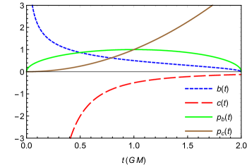
Figure 1: The behavior of canonical variables as a function of the Schwarzschild time $t$. We have chosen the positive sign for $b$ and negative sign for $c$. The figure is plotted using $\gamma=0.5,\,M=1,\,G=1$ and $L_{0}=1$.

The behavior of these solutions as a function of $t$ is depicted in Fig. 1. From these equations or the plot, one can see that $p_{c}\to 0$ as $t\to 0$, i.e., at the classical singularity. As a result Riemann invariants such as the Kretschmann scalar

$$K=R_{abcd}R^{abcd}\propto\frac{1}{p_{c}^{3}},$$ (33)

all diverge, signaling the presence of a physical singularity for $p_{c}\to 0$ as expected.

3 The classical Raychaudhuri Equation

Let a congruence of (a collection of nearby) geodesics be defined by the velocity field tangent to the geodesics, $u^{a}(x)$. Then taking the derivative of $u_{a;b}$ with respect to the proper time $\tau$ (or affine parameter), we get

$$\frac{du_{a;b}}{d\tau}=u_{a;b;c}\,u^{c}= \left[u_{a;c;b}+R_{cba}^{d}u_{a}\right]u^{c}$$

$$= (u_{a;c}u^{c})_{;b}-u_{;b}^{c}u_{a;c}+R_{cbad}u^{c}u^{d}.$$ (34)

Next, defining the induced metric $h_{ab}=g_{ab}-u_{a}u_{b}$, decomposing $u_{a;b}$ into its trace, symmetric and antisymmetric parts as follows $u_{a;b}=\frac{1}{3}\theta h_{ab}+\sigma_{ab}+\omega_{ab}$ and taking the trace of Eq. (34), we get

$$\frac{d\theta}{d\tau}=-\frac{1}{3}\,\theta^{2}-\sigma_{ab}\sigma^{ab}+\omega_{ab}\omega^{ab}-R_{ab}u^{a}u^{b}.$$ (35)

Here $\theta$ is the expansion, $\sigma_{ab}\sigma^{ab}$ is the shear, $\omega_{ab}\omega^{ab}$ is the vorticity term and $R_{ab}$ is the Ricci tensor. As can be seen, most of the terms in the RHS of the above equation are negative and therefore for a congruence of geodesics with no vorticity, the above equation can be integrated to give $\tau<3/\theta_{0}$, where $\theta_{0}$ is the initial value of $\theta$ and $\tau$ signifies the proper time of geodesic convergence. In the next few sections we will show how quantum corrections will introduce positive terms in the RHS of Eq. (35).

Since we consider our model in vacuum, we can set $R_{ab}=0$ in (35). Also, in general in KS models, the vorticity term is only nonvanishing if one considers metric perturbations Collins:1977fg . Hence, $\omega_{ab}\omega^{ab}=0$ in our model, too. This reduces the Raychaudhuri equation for our analysis to

$$\frac{d\theta}{d\tau}=-\frac{1}{3}\theta^{2}-\sigma_{ab}\sigma^{ab}.$$ (36)

It is well-known that the expansion and shear for this model can be written in terms of $N,\,p_{b},\,p_{c}$ and their time derivatives as Collins:1977fg ; Blanchette:2020kkk ; Bosso:2020ztk

$$\theta= \frac{\dot{p}_{b}}{Np_{b}}+\frac{\dot{p}_{c}}{2Np_{c}},$$ (37)

$$\sigma^{2}= \frac{2}{3}\left(-\frac{\dot{p}_{b}}{Np_{b}}+\frac{\dot{p}_{c}}{Np_{c}}\right)^{2}.$$ (38)

Replacing (25), (27) and (22) into (37) and (38) and substituting them into (36) we obtain Blanchette:2020kkk ; Bosso:2020ztk

$$\frac{d\theta}{d\tau}=-\frac{1}{2p_{c}}\left(1+\frac{9b^{2}}{2\gamma^{2}}+\frac{\gamma^{2}}{2b^{2}}\right).$$ (39)

Using (32) and (29) in the above yields Blanchette:2020kkk ; Bosso:2020ztk

$$\frac{d\theta}{d\tau}=\frac{-2t^{2}+8GMt-9G^{2}M^{2}}{\left(2GM-t\right)t^{3}}.$$ (40)

In the same way, one can obtain

$$\theta=\pm\frac{1}{2\sqrt{p_{c}}}\left(\frac{3b}{\gamma}-\frac{\gamma}{b}\right)=\pm\frac{-2t+3GM}{t^{\frac{3}{2}}\sqrt{(2GM-t)}}.$$ (41)

These expressions and their plot in Fig. 2 clearly signal the presence of a singularity at $t\to 0$ as expected.

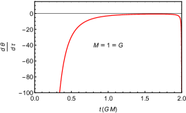
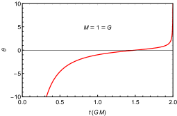
Figure 2: Left: $\frac{d\theta}{d\tau}$ as a function of the Schwarzschild time $t$. Right: negative branch of $\theta$ as a function of $t$. Both $\theta$ and $\frac{d\theta}{d\tau}$ diverge as we approach $t\to 0$. Note that the divergence at the horizon is due to the choice of Schwarzschild coordinate system.

4 General deformed algebra, Effective dynamics and the Raychaudhuri equation

As mentioned in the Introduction, various approaches to QG, black hole physics etc. strongly suggest the existence of a minimum measurable length in spacetime. This is often associated with the Planck length, but in principle can be any length scale lying between the Planck and the electroweak scale. This gives rise to an effective and generic modification of the standard Heisenberg algebra. Inspired by the above, and the fact that a corrected quantum algebra also implies suitable modifications of the corresponding Poisson algebra, we propose the following fundamental Poisson brackets between the canonical variables as

$$\{b,p_{b}\} =G\gamma F_{1}\left(b,c,p_{b},p_{c},\beta_{b},\beta_{c}\right),$$ (42)

$$\{c,p_{c}\} =2G\gamma F_{2}\left(b,c,p_{b},p_{c},\beta_{b},\beta_{c}\right),$$ (43)

where the modifications are encoded entirely in $F_{1}$ and $F_{2}$, and hence the non-deformed classical limit is obtained by setting $F_{1}=1=F_{2}$. Such modification will result in the effective equations of motion

$$\frac{db}{dT} =\{b,H\}=-\frac{1}{2}\left(b+\frac{\gamma^{2}}{b}\right)F_{1},$$ (44)

$$\frac{dp_{b}}{dT} =\{p_{b},H\}=\frac{p_{b}}{2}\left(1-\frac{\gamma^{2}}{b^{2}}\right)F_{1},$$ (45)

$$\frac{dc}{dT} =\{c,H\}=-2cF_{2},$$ (46)

$$\frac{dp_{c}}{dT} =\{p_{c},H\}=2p_{c}F_{2}.$$ (47)

As before, these equations should be supplemented by weakly vanishing of the Hamiltonian constraint (23).

From the above equations of motion for $b,\,p_{b}$, we can infer

$$\frac{db}{dp_{b}}=\frac{\left(\gamma^{2}+b^{2}\right)}{\left(\gamma^{2}-b^{2}\right)}\frac{b}{p_{b}}.$$ (48)

which leads to

$$p_{b}=\frac{Ab}{\gamma^{2}+b^{2}},$$ (49)

with $A$ being a constant of integration. In the same way from the equations of motion for $c,\,p_{c}$, we get

$$\frac{dc}{dp_{c}}=-\frac{c}{p_{c}},$$ (50)

which yields

$$p_{c}=\frac{B}{c},$$ (51)

with $B$ being another integration constant. From the last two equations we can also deduce a couple of basic results that will be useful later. First, note that if one demands that the Kretchmann scalar (33) remains finite everywhere inside the black hole, then $p_{c}$ should remain finite everywhere, and particularly at $t\to 0$. Hence, from Eq. (51) and assuming a finite $p_{c}$ everywhere in the interior, we deduce that $c$ should remain finite everywhere in the interior too. Second, from Eq. (49) we can have three types of behaviors for $b(t)$, particularly at $t\to 0$, as follows:

1. If for $t\to 0$ we get $b\to 0$, then $p_{b}\to 0$ too in that region.

2. If $b$ remains finite, then $p_{b}$ will remain finite.

3. If $b\to\pm\infty$, then $p_{b}\to 0$.

The above equations of motion (44)-(47) can now be substituted into the Raychaudhuri equation, Eq. (36) and (37) to obtain (with $N=\frac{\gamma\sqrt{p_{c}}}{b}$ as before):

$$\frac{d\theta}{d\tau}=\frac{1}{4\gamma^{2}p_{c}}\left(2\gamma^{2}F_{1}^{2}+4b^{2}F_{1}F_{2}-4\gamma^{2}F_{1}F_{2}-b^{2}F_{1}^{2}-12b^{2}F_{2}^{2}-\frac{F_{1}^{2}\gamma^{4}}{b^{2}}\right),$$ (52)

and

$$\theta=\pm\frac{1}{2\gamma\sqrt{p_{c}}}\left(bF_{1}-\frac{\gamma^{2}F_{1}}{b}+2bF_{2}\right),$$ (53)

in terms of the canonical variables. We need both $\theta$ and $\frac{d\theta}{d\tau}$ to remain finite everywhere, particularly close to and at the singularity. Since we are assuming $p_{c}|_{t\to 0}\to\mathrm{finite}$ due to requirement for finiteness of the Kretchmann scalar at the singularity, only the terms inside the parentheses in $\theta$ and $\frac{d\theta}{d\tau}$ above matter.

In what follows, we will consider four cases of linear modifications to the Poisson algebra. These cases, as suggested by literature in the field, are the most used cases in GUP-inspired models. These cases include the configuration-dependent modifications

$$F_{1}(q,p)= 1+\alpha_{b}b, F_{2}(q,p)= 1+\alpha_{c}c,$$ (54)

$$F_{1}(q,p)= 1+\beta_{b}b^{2}, F_{2}(q,p)= 1+\beta_{c}c^{2},$$ (55)

and the momentum-dependent modifications

$$F_{1}(q,p)= 1+\alpha_{b}^{\prime}p_{b}, F_{2}(q,p)= 1+\alpha_{c}^{\prime}p_{c},$$ (56)

$$F_{1}(q,p)= 1+\beta_{b}^{\prime}p_{b}^{2}, F_{2}(q,p)= 1+\beta_{c}^{\prime}p_{c}^{2}.$$ (57)

In what follows we consider the effect of such modifications on the dynamics of the interior and the behavior of $\theta$ and $\frac{d\theta}{d\tau}$ in this region.

5 Specific models

We consider four distinct GUP inspired models in this section and examine the consequences. These four models are chosen because they cover most of the spectrum of GUPs that authors have used to study Planck scale/QG corrections in quantum systems, suitably adapted to the problem at hand. Following the lead of those works studying linear and quadratic GUP models, our four cases cover the linear and quadratic in the canonical variables $b,c,p_{b}$ and $p_{c}$.

5.1 Model 1: $F_{1}=1+\beta_{b}b^{2},\,F_{2}=1+\beta_{c}c^{2}$

This is the case whose dynamics was studies in Bosso:2020ztk . Here, the algebra becomes

$$\left\{b,p_{b}\right\}= G\gamma\left(1+\beta_{b}b^{2}\right),$$ (58)

$$\left\{c,p_{c}\right\}= 2G\gamma\left(1+\beta_{c}c^{2}\right),$$ (59)

and the corresponding equations of motion are

$$\frac{db}{dT}= \left\{b,H\right\}=-\frac{1}{2}\left(b+\frac{\gamma^{2}}{b}\right)\left(1+\beta_{b}b^{2}\right),$$ (60)

$$\frac{dp_{b}}{dT}= \left\{p_{b},H\right\}=\frac{p_{b}}{2}\left(1-\frac{\gamma^{2}}{b^{2}}\right)\left(1+\beta_{b}b^{2}\right),$$ (61)

$$\frac{dc}{dT}= \left\{c,H\right\}=-2c\left(1+\beta_{c}c^{2}\right),$$ (62)

$$\frac{dp_{c}}{dT}= \left\{b,H\right\}=2p_{c}\left(1+\beta_{c}c^{2}\right).$$ (63)

Once again, these equations should be supplemented by the weakly vanishing ($\approx 0$) of the Hamiltonian constraint (23),

$$\left(b^{2}+\gamma^{2}\right)\frac{p_{b}}{b}+2cp_{c}\approx 0.$$ (64)

The solutions to these equations of motion in terms of the Schwarzschild time $t$ are Bosso:2020ztk

$$b\left(t\right)= \pm\frac{\gamma\sqrt{2GMt^{\beta_{b}\gamma^{2}}-t\left(2\gamma^{2}GM\right)^{\beta_{b}\gamma^{2}}}}{\sqrt{t\left(2\gamma^{2}GM\right)^{\beta_{b}\gamma^{2}}-2\beta_{b}\gamma^{2}GMt^{\beta_{b}\gamma^{2}}}},$$ (65)

$$p_{b}\left(t\right)= \frac{\ell_{c}}{\sqrt{-\beta_{c}}}t^{-\beta_{b}\gamma^{2}}\sqrt{\left[2GMt^{\beta_{b}\gamma^{2}}-t\left(2\gamma^{2}GM\right)^{\beta_{b}\gamma^{2}}\right]\left[t\left(2\gamma^{2}GM\right)^{\beta_{b}\gamma^{2}}-2\beta_{b}\gamma^{2}GMt^{\beta_{b}\gamma^{2}}\right]},$$ (66)

$$c\left(t\right)= \mp\frac{\ell_{c}}{\sqrt{-\beta_{c}}}\frac{\gamma GM}{\sqrt{t^{4}-\ell_{c}^{2}\gamma^{2}G^{2}M^{2}}},$$ (67)

$$p_{c}\left(t\right)= \sqrt{t^{4}+\ell_{c}^{2}\gamma^{2}G^{2}M^{2}}.$$ (68)

where we have set $l=1$. Following Bosso:2020ztk , in these equations we have defined a physical scale

$$\ell_{c}^{2}=-\beta_{c}L_{0}^{2}.$$ (69)

The introduction of this scale is necessary to avoid the dependence of physical quantities such as expansion and shear on the fiducial parameter $L_{0}$. Note that if we identify this $p_{c}^{\mathrm{min}}$ with the one derived from LQG in Corichi:2015xia , we will obtain $\ell_{c}^{(\alpha)2}=\Delta$ Bosso:2020ztk , where $\Delta$ is the minimum area in LQG.

The above solutions are plotted in Fig. 3. In general:

• If $\beta_{c}<0$ then $p_{c}$ never vanishes, and hence the Kretschmann scalar does not diverge. Consequently the singularity is resolved effectively. Also in this case $c$ becomes bounded everywhere in the interior.

• If $\beta_{b}<0$ then $b$ is bounded everywhere in the interior.

• If $\beta_{c}=0$, then $p_{c}\to 0$ for $t\to 0$ and the Kretchamnn scalar blows up in that region. Hence, singularity will be still present. Also in this case $c$ will not be bounded.

• If $\beta_{b}\geq 0$, then $b$ will not be bounded.

• If $\beta_{c}>0$, then the evolution stops at some point before reaching $t=0$ due to $p_{c}$ becoming complex. Also (69) will not make sence for a real scale $\ell_{c}$.

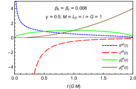
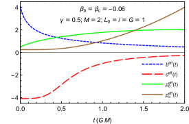
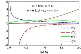
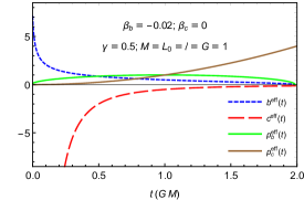
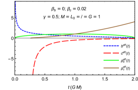
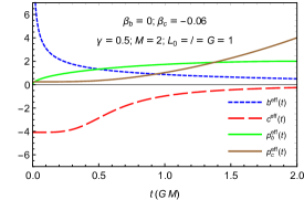
Figure 3: The behavior of solutions of the modified case in the Schwarzschild time $t$ for positive, negative and vanishing $\beta_{b}$ and $\beta_{c}$ for the whole interior. We have chosen the positive sign for $b$ and negative sign for $c$. Note that for nonvanishing negative $\beta_{c}$ we always get a minimum nonvanishing value for $p_{c}$, while a nonvanishing negative $\beta_{b}$ leads to a finite value of $b$ at $t\to 0$. The values of parameters are mentioned on each plot.

Therefore we can conclude that the case of interest for us is the one in which both $\beta_{b},\,\beta_{c}<0$ (top right plot). In this case not only $p_{c}$ acquires a minimum value and the Kretchmann scalar remains finite, but also $b$ and $c$ are bounded.

From the solution (65) (also seen in Fig 3), and assuming since $\beta_{b},\,\beta_{c}<0$, we see that

$$b|_{t\to 0^{+}}\to \frac{1}{\sqrt{-\beta_{b}}},$$ (70)

$$F_{1}|_{t\to 0^{+}}\to 0,$$ (71)

$$F_{2}|_{t\to 0^{+}}\to 0.$$ (72)

Considering these limits and looking at (52) and (53), we see that both $\theta$ and $\frac{d\theta}{d\tau}$ vanish at $t\to 0$. This in fact can be seen by computing the expression for the expansion

$$\theta=\frac{1}{2\gamma\sqrt{p_{c}}}\left[3b-\frac{\gamma^{2}}{b}+\beta_{b}b\left(b^{2}-\gamma^{2}\right)+2\beta_{c}c^{2}b\right],$$ (73)

and the Raychaudhuri equation Bosso:2020ztk ,

$$\frac{d\theta}{d\tau}= -\frac{9b^{2}}{4\gamma^{2}p_{c}}-\frac{\gamma^{2}}{4b^{2}p_{c}}-\frac{1}{2p_{c}}$$

$$+\frac{\beta_{b}}{2\gamma^{2}p_{c}}\left(b^{4}-\gamma^{4}\right)-\frac{\beta_{c}c^{2}}{\gamma^{2}p_{c}}\left(5b^{2}+\gamma^{2}\right)$$

$$-\frac{\beta_{b}^{2}b^{2}}{4\gamma^{2}p_{c}}\left(b^{2}-\gamma^{2}\right)^{2}-\frac{3b^{2}\beta_{c}^{2}c^{4}}{\gamma^{2}p_{c}}+\frac{\beta_{b}\beta_{c}b^{2}c^{2}}{\gamma^{2}p_{c}}\left(b^{2}-\gamma^{2}\right),$$ (74)

for this model, and then replacing in them the solutions (65)-(68) for $\beta_{b},\beta_{c}<0$ and plotting them versus the Schwarzschild time $t$. These plots are presented in Fig. 4, in which one can compare the behavior of effective $\theta$ and $\frac{d\theta}{d\tau}$ versus their classical counterparts. We see that far from the the position where used to be the classical singularity, the effective behavior follows the classical one almost identically. However, close to the $t=0$ region, the defocusing effective corrections dominate and prevent $\theta$ and $\frac{d\theta}{d\tau}$ from diverging. This shows that the singularity is resolved in the effective regime. Furthermore, interestingly $\frac{d\theta}{d\tau}$ shows a similar qualitative behavior (double bump) as the $\bar{\mu}$ case in (most of) the loop quantum gravity approach(es) to this model (Fig. 8 in Blanchette:2020kkk ).

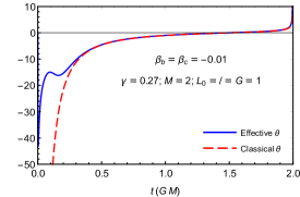
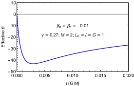
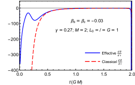
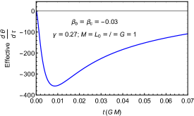
Figure 4: Plots of expansion and its rate of change for model 1. Top left: classical vs effective $\theta$ as a function of the Schwarzschild time $t$. Top right: closeup of the effective $\theta$ as a function of $t$. Bottom left: classical vs effective $\frac{d\theta}{d\tau}$ as a function of $t$. Top right: closeup of the effective $\frac{d\theta}{d\tau}$ as a function of $t$.

5.2 Model 2: $F_{1}=1+\beta_{b}^{\prime}p_{b}^{2},\,F_{2}=1+\beta_{c}^{\prime}p_{c}^{2}$

In this case, once $F_{1},\,F_{2}$ are replaced into (44)-(47), it is possible to analytically solve the equation in $c,\,p_{c}$ in Schwarzschild time $t$,

$$c= GMlL_{0}\gamma\frac{\sqrt{1-\beta_{c}^{\prime}t^{4}}}{t^{2}},$$ (75)

$$p_{c}= \frac{t^{2}}{\sqrt{1-\beta_{c}^{\prime}t^{4}}},$$ (76)

where first we have solved the differential equations in $T$, replaced $T\to\ln\left(t\right)$ and then matched the classical limits the known classical solutions Eqs. (29)-(32). Immediately, we see from (76) that

$$\lim_{t\to 0^{+}}p_{c}=0,$$ (77)

and hence the Kretchmann scalar diverges at $t\to 0$ and singularity is not resolved even in the effective regime. Furthermore $c$ blows up at $t\to 0$. So we will not further analyze the behavior of $\theta$ and $\frac{d\theta}{d\tau}$ in this case.

5.3 Model 3 $F_{1}=1+\alpha_{b}b,\,F_{2}=1+\alpha_{c}c$

For this model, too, it is possible to analytically solve for $c,\,p_{c}$, while $b,\,p_{b}$ can be obtained numerically. For $c,\,p_{c}$ we obtain

$$c= -\frac{GM\gamma lL_{0}}{t^{2}+\alpha_{c}GM\gamma lL_{0}},$$ (78)

$$p_{c}= t^{2}+\alpha_{c}GM\gamma lL_{0}.$$ (79)

This shows that $p_{c}$ at $t\to 0$ acquires a minimum which depends on $L_{0}$. Once again we can use the prescription introduced in Bosso:2020ztk to define a new physical scale

$$\ell_{c}^{(\alpha)}=\alpha_{c}L_{0},$$ (80)

and thus the minimum values of $p_{c}$ becomes

$$p_{c}^{\mathrm{min}}=\ell_{c}^{(\alpha)}GM\gamma.$$ (81)

Again, if we identify this $p_{c}^{\mathrm{min}}$ with the one derived from LQG in Corichi:2015xia , we will once again obtain $\ell_{c}^{(\alpha)2}=\Delta$.

Using the solutions above, we see that at $t\to 0$

$$c=-\frac{1}{\alpha_{c}},$$ (82)

and hence

$$F_{2}|_{t\to 0}=0.$$ (83)

Replacing these forms of $F_{1}$ and $F_{2}$ in (53) and (52) yields

$$\theta|_{t\to 0}= \frac{1}{2\gamma\sqrt{p_{c}}}\left(b^{2}-\gamma^{2}\right)\frac{F_{1}}{b}$$

$$= \frac{1}{2\gamma\sqrt{p_{c}}}\left(b^{2}-\gamma^{2}\right)\left(\alpha_{b}+\frac{1}{b}\right),$$ (84)

and

$$\frac{d\theta}{d\tau}\bigg{|}_{t\to 0}= -\frac{1}{4\gamma^{2}p_{c}}\left(b^{2}-\gamma^{2}\right)^{2}\left(\frac{F_{1}}{b}\right)^{2}$$

$$= -\frac{1}{4\gamma^{2}p_{c}}\left[\left(b^{2}-\gamma^{2}\right)\left(\alpha_{b}+\frac{1}{b}\right)\right]^{2}$$

$$= -\left[\theta|_{t\to 0}\right]^{2}.$$ (85)

It is clear from above two equations that the only way to keep both $\theta$ and $\frac{d\theta}{d\tau}$ finite is for $b$ to remain finite at $t\to 0$.

We can see these results in another way. By replacing $c$ from (51) in $F_{2}$ we obtain

$$F_{2}=1+\alpha_{c}\frac{B}{p_{c}}.$$ (86)

Substituting both of the above $F_{1},\,F_{2}$ in (53) and (52) one obtains

$$\theta=\frac{1}{2\gamma\sqrt{p_{c}}}\left[3b-\frac{\gamma^{2}}{b}+\alpha_{b}\left(b^{2}-\gamma^{2}\right)+\alpha_{c}\frac{2bB}{p_{c}}\right],$$ (87)

and

$$\frac{d\theta}{d\tau}= -\frac{9b^{2}}{4\gamma^{2}p_{c}}-\frac{\gamma^{2}}{4b^{2}p_{c}}-\frac{1}{2p_{c}}$$

$$+\frac{\alpha_{b}}{\gamma^{2}bp_{c}}\left(b^{4}-\gamma^{4}\right)-\frac{B\alpha_{c}}{\gamma^{2}p_{c}^{2}}\left(5b^{2}+\gamma^{2}\right)$$

$$-\frac{\alpha_{b}^{2}}{4\gamma^{2}p_{c}}\left(b^{2}-\gamma^{2}\right)^{2}-\frac{3b^{2}B^{2}\alpha_{c}^{2}}{\gamma^{2}p_{c}^{3}}+\frac{B\alpha_{b}\alpha_{c}b}{\gamma^{2}p_{c}^{2}}\left(b^{2}-\gamma^{2}\right).$$ (88)

From these two expressions we see that a necessary and sufficient condition for finiteness of both $\theta$ and $\frac{d\theta}{d\tau}$ is the finiteness of $b$ when $t\to 0$. Also note the similarity of this expression with Eq. (74) from model 1. From the discussion in Sec. 4, the finiteness of $b$ means that all the four canonical variables should remain finite at $t\to 0$ for both $\theta$ and $\frac{d\theta}{d\tau}$ not to diverge. This is in fact the case as we will see below.

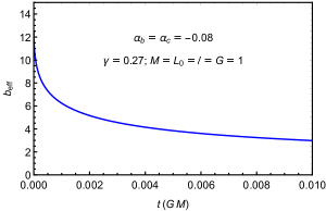
Figure 5: Plot of the solution for $b$ as a function of the Schwarzschild time $t$ for model 3 close to the region that used to be the singularity. It is clear that $b$ remains finite as $t\to 0^{+}$.

The above analysis is confirmed by numerical solutions of the differential equations for $b,\,p_{b}$ in this case. From these numerical solutions, particularly the one for $b$ which is plotted in Fig 5, it is clear that $b$ is bounded in the interior and especially for $t\to 0^{+}$.

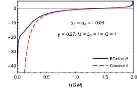
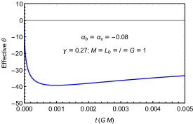
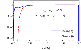
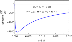
Figure 6: Plots of expansion and its rate of change for model 3. Top left: classical vs effective $\theta$ as a function of the Schwarzschild time $t$. Top right: closeup of the effective $\theta$ as a function of $t$. Bottom left: classical vs effective $\frac{d\theta}{d\tau}$ as a function of $t$. Top right: closeup of the effective $\frac{d\theta}{d\tau}$ as a function of $t$.

Furthermore, by using the numerical solutions for $b,\,p_{b}$ and the analytical solutions for $c,\,p_{c}$ in expressions (87) and (88) for $\theta$ and $\frac{d\theta}{d\tau}$, one can obtain the plot of these quantities. These are presented in Fig. 6. Once again we see that far from the position where used to be the classical singularity, the classical and the effective quantities matc almost exactly. However, as $t\to 0$, the effective terms take over and turn the expansion and its rate toward the value zero. Also note that once again the double bump pattern is visible in the plot of $\frac{d\theta}{d\tau}$.

5.4 Model 4: $F_{1}=1+\alpha_{b}^{\prime}p_{b},\,F_{2}=1+\alpha_{c}^{\prime}p_{c}$

For this case, the solutions to $c,\,p_{c}$ in $t$ are

$$c= -GM\gamma lL_{0}\frac{1-\alpha_{c}^{\prime}t^{2}}{t^{2}},$$ (89)

$$p_{c}= \frac{t^{2}}{1-\alpha_{c}^{\prime}t^{2}}.$$ (90)

Hence, similar to Model 2, we have $\lim_{t\to 0^{+}}p_{c}=0$ and the Kretschmann scalar blows up at $t\to 0$. Therefore, the singularity persists even in the effective GUP regime.

6 Discussion and conclusion

In this work, we have studied the effects of modifying the Poisson bracket inspired by GUP on the Raychaudhuri equation in the interior of the Schwarzschild black hole. This modification leads to an effective algebra that can be interpreted as a modification inherited from the quantum algebra. As a result, the equations of motion will be modified and give us an effective dynamics in the interior of the black hole.

We have first studied a generic class of modifications and analyzed the conditions under which the expansion scalar $\theta$ and its rate of change $\frac{d\theta}{d\tau}$, i.e., the Raychaudhuri equation, remain finite everywhere inside the black hole. This finiteness signals the absence of caustic points and particularly in this case, a physical singularity.

Armed with such a generic analysis, we studied four specific models that is usually considered in GUP theories with linear or quadratic mortification to the algebra. We studied their effective dynamics and analyzed in detail, the behavior of $\theta$ and $\frac{d\theta}{d\tau}$ in each model. We have shown that in two of these models, in which the modifications are momentum dependent, the singularity persists. However, in the other two model which are either linearly or quadratically dependent of the configuration variables, due to quantum gravity correction, the Kretchamann scalar, $\theta$ and $\frac{d\theta}{d\tau}$ remain finite everywhere inside the black hole. This is a strong indication that the singularity of the black hole is resolved effectively. In addition to being finite, both $\theta$ and $\frac{d\theta}{d\tau}$ approach zero as the Schwarzschild time $t\to 0$.

The main reason for the aforementioned behavior of $\theta$ and $\frac{d\theta}{d\tau}$ is the following: in the interior of the Schwarzschild black hole which is a special form of the Kantowski-Sachs cosmological model, both $\theta$ and $\frac{d\theta}{d\tau}$ depend on the time derivatives of the momenta of the model. Replacing these time derivatives from the classical equations of motion into the expressions for $\theta$ and $\frac{d\theta}{d\tau}$ leads to terms that all have negative terms, implying focusing of the geodesics which ultimately lead to caustic points with $\theta,\,\frac{d\theta}{d\tau}\to-\infty$ for $t\to 0^{+}$. This is not surprising given the attractive nature of gravity. However, repeating the same procedure but now suing the effective equations of motion leads to two sets of terms. The classical ones that are all negative as before and terms coming from the modifications that are positive. These terms are quite small far from $t\to 0^{+}$ but dominate and take over close to that region and turn the values of $\theta$ and $\frac{d\theta}{d\tau}$ over to zero rather than $-\infty$. One can effective interpret these terms as repulsive.

Although the models we consider here do not exhaust all possibilities and other GUP models can be considered in principle, as mentioned earlier, the models we study here are the ones that are more frequently studied in the literature. Having said that, for the sake of completeness and to shed more light on other GUP models, it is worth examining them in the future.

As a future project, we would like to extend our results to more general spacetimes. In particular, we would like to study the form of modifications to a generic class of metrics needed for the singularity to be resolved especially in relation to the behavior of $\theta$ and $\frac{d\theta}{d\tau}$.

- (1) A. Raychaudhuri, Relativistic cosmology. 1., Phys. Rev. 98 (1955) 1123.
- (2) R. Penrose, Gravitational collapse and space-time singularities, Phys. Rev. Lett. 14 (1965) 57.
- (3) S. Hawking and R. Penrose, The Singularities of gravitational collapse and cosmology, Proc. Roy. Soc. Lond. A 314 (1970) 529.
- (4) T. Thiemann, Modern Canonical Quantum General Relativity, Cambridge Monographs on Mathematical Physics. Cambridge University Press, 2007, 10.1017/CBO9780511755682.
- (5) M. Bojowald, Spherically symmetric quantum geometry: States and basic operators, Class. Quant. Grav. 21 (2004) 3733 [gr-qc/0407017].
- (6) A. Ashtekar and M. Bojowald, Quantum geometry and the Schwarzschild singularity, Class. Quant. Grav. 23 (2006) 391 [gr-qc/0509075].
- (7) M. Bojowald and R. Swiderski, Spherically symmetric quantum geometry: Hamiltonian constraint, Class. Quant. Grav. 23 (2006) 2129 [gr-qc/0511108].
- (8) Böhmer, Christian G. and Vandersloot, Kevin, Loop Quantum Dynamics of the Schwarzschild Interior, Phys. Rev. D 76 (2007) 104030 [0709.2129].
- (9) A. Corichi and P. Singh, Loop quantization of the Schwarzschild interior revisited, Class. Quant. Grav. 33 (2016) 055006 [1506.08015].
- (10) A. Barrau, K. Martineau and F. Moulin, A status report on the phenomenology of black holes in loop quantum gravity: Evaporation, tunneling to white holes, dark matter and gravitational waves, Universe 4 (2018) 102 [1808.08857].
- (11) E. Alesci, S. Bahrami and D. Pranzetti, Quantum gravity predictions for black hole interior geometry, Phys. Lett. B 797 (2019) 134908 [1904.12412].
- (12) D. Arruga, J. Ben Achour and K. Noui, Deformed General Relativity and Quantum Black Holes Interior, Universe 6 (2020) 39 [1912.02459].
- (13) N. Bodendorfer, F. M. Mele and J. Münch, Effective Quantum Extended Spacetime of Polymer Schwarzschild Black Hole, Class. Quant. Grav. 36 (2019) 195015 [1902.04542].
- (14) S. Brahma, Spherically symmetric canonical quantum gravity, Phys. Rev. D 91 (2015) 124003 [1411.3661].
- (15) M. Campiglia, R. Gambini and J. Pullin, Loop quantization of spherically symmetric midi-superspaces : The Interior problem, AIP Conf. Proc. 977 (2008) 52 [0712.0817].
- (16) D.-W. Chiou, Phenomenological loop quantum geometry of the Schwarzschild black hole, Phys. Rev. D 78 (2008) 064040 [0807.0665].
- (17) A. Corichi, A. Karami, S. Rastgoo and T. Vukašinac, Constraint Lie algebra and local physical Hamiltonian for a generic 2D dilatonic model, Class. Quant. Grav. 33 (2016) 035011 [1508.03036].
- (18) J. Cortez, W. Cuervo, H. A. Morales-Técotl and J. C. Ruelas, Effective loop quantum geometry of Schwarzschild interior, Phys. Rev. D 95 (2017) 064041 [1704.03362].
- (19) R. Gambini and J. Pullin, Black holes in loop quantum gravity: The Complete space-time, Phys. Rev. Lett. 101 (2008) 161301 [0805.1187].
- (20) R. Gambini, J. Pullin and S. Rastgoo, Quantum scalar field in quantum gravity: The vacuum in the spherically symmetric case, Class. Quant. Grav. 26 (2009) 215011 [0906.1774].
- (21) R. Gambini, J. Pullin and S. Rastgoo, Quantum scalar field in quantum gravity: the propagator and Lorentz invariance in the spherically symmetric case, Gen. Rel. Grav. 43 (2011) 3569 [1105.0667].
- (22) R. Gambini and J. Pullin, Loop quantization of the Schwarzschild black hole, Phys. Rev. Lett. 110 (2013) 211301 [1302.5265].
- (23) R. Gambini, J. Olmedo and J. Pullin, Spherically symmetric loop quantum gravity: analysis of improved dynamics, Class. Quant. Grav. 37 (2020) 205012 [2006.01513].
- (24) V. Husain and O. Winkler, Quantum resolution of black hole singularities, Class. Quant. Grav. 22 (2005) L127 [gr-qc/0410125].
- (25) J. G. Kelly, R. Santacruz and E. Wilson-Ewing, Effective loop quantum gravity framework for vacuum spherically symmetric space-times, 2006.09302.
- (26) T. Thiemann and H. Kastrup, Canonical quantization of spherically symmetric gravity in Ashtekar’s selfdual representation, Nucl. Phys. B 399 (1993) 211 [gr-qc/9310012].
- (27) M. Campiglia, R. Gambini and J. Pullin, Loop quantization of spherically symmetric midi-superspaces, Class. Quant. Grav. 24 (2007) 3649 [gr-qc/0703135].
- (28) R. Gambini, J. Pullin and S. Rastgoo, New variables for 1+1 dimensional gravity, Class. Quant. Grav. 27 (2010) 025002 [0909.0459].
- (29) S. Rastgoo, A local true Hamiltonian for the CGHS model in new variables, 1304.7836.
- (30) A. Corichi, J. Olmedo and S. Rastgoo, Callan-Giddings-Harvey-Strominger vacuum in loop quantum gravity and singularity resolution, Phys. Rev. D 94 (2016) 084050 [1608.06246].
- (31) H. A. Morales-Técotl, S. Rastgoo and J. C. Ruelas, Effective dynamics of the Schwarzschild black hole interior with inverse triad corrections, Annals Phys. 426 (2021) 168401 [1806.05795].
- (32) K. Blanchette, S. Das, S. Hergott and S. Rastgoo, Black hole singularity resolution via the modified Raychaudhuri equation in loop quantum gravity, Phys. Rev. D 103 (2021) 084038 [2011.11815].
- (33) A. Ashtekar, S. Fairhurst and J. L. Willis, Quantum gravity, shadow states, and quantum mechanics, Class. Quant. Grav. 20 (2003) 1031 [gr-qc/0207106].
- (34) A. Corichi, T. Vukasinac and J. A. Zapata, Polymer Quantum Mechanics and its Continuum Limit, Phys. Rev. D 76 (2007) 044016 [0704.0007].
- (35) H. A. Morales-Técotl, S. Rastgoo and J. C. Ruelas, Path integral polymer propagator of relativistic and nonrelativistic particles, Phys. Rev. D 95 (2017) 065026 [1608.04498].
- (36) H. A. Morales-Técotl, D. H. Orozco-Borunda and S. Rastgoo, Polymer quantization and the saddle point approximation of partition functions, Phys. Rev. D 92 (2015) 104029 [1507.08651].
- (37) E. Flores-González, H. A. Morales-Técotl and J. D. Reyes, Propagators in Polymer Quantum Mechanics, Annals Phys. 336 (2013) 394 [1302.1906].
- (38) D. Amati, M. Ciafaloni and G. Veneziano, Can Space-Time Be Probed Below the String Size?, Phys. Lett. B 216 (1989) 41.
- (39) D. J. Gross and P. F. Mende, String Theory Beyond the Planck Scale, Nucl. Phys. B 303 (1988) 407.
- (40) G. AMELINO-CAMELIA, Relativity in spacetimes with short-distance structure governed by an observer-independent (planckian) length scale, International Journal of Modern Physics D 11 (2002) 35–59.
- (41) G. Amelino-Camelia, Testable scenario for relativity with minimum length, Physics Letters B 510 (2001) 255–263.
- (42) J. L. Cortés and J. Gamboa, Quantum uncertainty in doubly special relativity, Physical Review D 71 (2005) .
- (43) I. Pikovski, M. R. Vanner, M. Aspelmeyer, M. S. Kim and v. Brukner, Probing planck-scale physics with quantum optics, Nature Physics 8 (2012) 393–397.
- (44) F. Marin et al., Gravitational bar detectors set limits to Planck-scale physics on macroscopic variables, Nature Phys. 9 (2013) 71.
- (45) M. Bawaj, C. Biancofiore, M. Bonaldi, F. Bonfigli, A. Borrielli, G. Di Giuseppe et al., Probing deformed commutators with macroscopic harmonic oscillators, Nature Communications 6 (2015) .
- (46) G. Amelino-Camelia, Quantum-spacetime phenomenology, Living Reviews in Relativity 16 (2013) .
- (47) S. Hossenfelder, Minimal length scale scenarios for quantum gravity, Living Reviews in Relativity 16 (2013) .
- (48) A. Kempf, G. Mangano and R. B. Mann, Hilbert space representation of the minimal length uncertainty relation, Phys. Rev. D 52 (1995) 1108 [hep-th/9412167].
- (49) M. Maggiore, A Generalized uncertainty principle in quantum gravity, Phys. Lett. B 304 (1993) 65 [hep-th/9301067].
- (50) M. Maggiore, Quantum groups, gravity, and the generalized uncertainty principle, Physical Review D 49 (1994) 5182–5187.
- (51) R. J. Adler, P. Chen and D. I. Santiago, The generalized uncertainty principle and black hole remnants, General Relativity and Gravitation 33 (2001) 2101–2108.
- (52) S. Das and E. C. Vagenas, Universality of quantum gravity corrections, Physical Review Letters 101 (2008) .
- (53) K. Nozari and S. H. Mehdipour, Quantum gravity and recovery of information in black hole evaporation, EPL (Europhysics Letters) 84 (2008) 20008.
- (54) A. Alonso-Serrano, M. P. Dąbrowski and H. Gohar, Generalized uncertainty principle impact onto the black holes information flux and the sparsity of hawking radiation, Physical Review D 97 (2018) .
- (55) Y. S. Myung, Y.-W. Kim and Y.-J. Park, Black hole thermodynamics with generalized uncertainty principle, Physics Letters B 645 (2007) 393–397.
- (56) P. Bargueño and E. C. Vagenas, Semiclassical corrections to black hole entropy and the generalized uncertainty principle, Physics Letters B 742 (2015) 15–18.
- (57) S. Gangopadhyay and A. Dutta, Black hole thermodynamics and generalized uncertainty principle with higher order terms in momentum uncertainty, Advances in High Energy Physics 2018 (2018) 1–9.
- (58) A. F. Ali and B. Majumder, Towards a cosmology with minimal length and maximal energy, Classical and Quantum Gravity 31 (2014) 215007.
- (59) A. F. Ali, M. Faizal and M. M. Khalil, Short distance physics of the inflationary de sitter universe, Journal of Cosmology and Astroparticle Physics 2015 (2015) 025–025.
- (60) S. Das and R. Mann, Planck scale effects on some low energy quantum phenomena, Physics Letters B 704 (2011) 596–599.
- (61) M. Sprenger, P. Nicolini and M. Bleicher, Neutrino oscillations as a novel probe for a minimal length, Classical and Quantum Gravity 28 (2011) 235019.
- (62) A. F. Ali, S. Das and E. C. Vagenas, Proposal for testing quantum gravity in the lab, Physical Review D 84 (2011) .
- (63) C. Rovelli and L. Smolin, Discreteness of area and volume in quantum gravity, Nucl. Phys. B 442 (1995) 593 [gr-qc/9411005].
- (64) L. J. Garay, Quantum gravity and minimum length, Int. J. Mod. Phys. A 10 (1995) 145 [gr-qc/9403008].
- (65) F. Scardigli, Generalized uncertainty principle in quantum gravity from micro - black hole Gedanken experiment, Phys. Lett. B 452 (1999) 39 [hep-th/9904025].
- (66) G. Amelino-Camelia, Quantum-Spacetime Phenomenology, Living Rev. Rel. 16 (2013) 5 [0806.0339].
- (67) P. Bosso, S. Das and R. B. Mann, Potential tests of the Generalized Uncertainty Principle in the advanced LIGO experiment, Phys. Lett. B 785 (2018) 498 [1804.03620].
- (68) P. Bosso, Generalized Uncertainty Principle and Quantum Gravity Phenomenology, Ph.D. thesis, Lethbridge U., 2017. 1709.04947.
- (69) P. Bosso, Rigorous Hamiltonian and Lagrangian analysis of classical and quantum theories with minimal length, Phys. Rev. D 97 (2018) 126010 [1804.08202].
- (70) P. Bosso and O. Obregón, Minimal length effects on quantum cosmology and quantum black hole models, Class. Quant. Grav. 37 (2020) 045003 [1904.06343].
- (71) R. Casadio and F. Scardigli, Generalized uncertainty principle, classical mechanics, and general relativity, Physics Letters B 807 (2020) 135558.
- (72) P. Bosso, On the quasi-position representation in theories with a minimal length, Class. Quant. Grav. 38 (2021) 075021 [2005.12258].
- (73) V. Todorinov, P. Bosso and S. Das, Relativistic generalized uncertainty principle, Annals of Physics 405 (2019) 92–100.
- (74) P. Bosso, S. Das and V. Todorinov, Quantum field theory with the generalized uncertainty principle i: Scalar electrodynamics, Annals of Physics 422 (2020) 168319.
- (75) P. Bosso, S. Das and V. Todorinov, Quantum field theory with the generalized uncertainty principle ii: Quantum electrodynamics, Annals of Physics 424 (2021) 168350.
- (76) Y. Bonder, A. Garcia-Chung and S. Rastgoo, Bounds on the Polymer Scale from Gamma Ray Bursts, Phys. Rev. D96 (2017) 106021 [1704.08750].
- (77) A. Das, S. Das and E. C. Vagenas, Discreteness of space from gup in strong gravitational fields, Physics Letters B 809 (2020) 135772.
- (78) A. Das, S. Das, N. R. Mansour and E. C. Vagenas, Bounds on gup parameters from gw150914 and gw190521, 2021.
- (79) A. Garcia-Chung, J. B. Mertens, S. Rastgoo, Y. Tavakoli and P. Vargas Moniz, Propagation of quantum gravity-modified gravitational waves on a classical FLRW spacetime, Phys. Rev. D 103 (2021) 084053 [2012.09366].
- (80) D. J. Stargen, S. Shankaranarayanan and S. Das, Polymer quantization and advanced gravitational wave detector, Physical Review D 100 (2019) .
- (81) S. Das and M. Fridman, Test of quantum gravity in statistical mechanics, 2021.
- (82) P. Bosso, O. Obregón, S. Rastgoo and W. Yupanqui, Deformed algebra and the effective dynamics of the interior of black holes, 2012.04795.
- (83) P. Bosso, O. Obregón, S. Rastgoo and W. Yupanqui, In preparation .
- (84) S. Das, Quantum raychaudhuri equation, Physical Review D 89 (2014) .
- (85) S. Das and R. K. Bhaduri, Dark matter and dark energy from a bose–einstein condensate, Classical and Quantum Gravity 32 (2015) 105003.
- (86) D. J. Burger, N. Moynihan, S. Das, S. S. Haque and B. Underwood, Towards the raychaudhuri equation beyond general relativity, Physical Review D 98 (2018) .
- (87) S. Das, S. S. Haque and B. Underwood, Constraints and horizons for de sitter with extra dimensions, Physical Review D 100 (2019) .
- (88) C. Collins, Global structure of the Kantowski-Sachs cosmological models, J. Math. Phys. 18 (1977) 2116.