Fermionic corrections to quark and gluon form factors in four-loop QCD

Abstract

We analytically compute all four-loop QCD corrections to the photon-quark and Higgs-gluon form factors involving a closed massless fermion loop. Our calculation of non-planar vertex integrals confirms a previous conjecture for the analytical form of the non-fermionic contributions to the collinear anomalous dimensions of quarks and gluons.

I Introduction

Two of the most important processes which are studied in great detail at the CERN LHC are the production of lepton pairs and Higgs bosons. The total cross sections for Drell-Yan lepton pair production through virtual photons and Higgs boson production through the dominant gluon fusion channel are known to next-to-next-to-next-to-leading order (N³LO) in perturbation theory [1, 2, 3] in the limit of an infinitely heavy top quark. Historically, first the virtual corrections have been computed and the real radiation contributions have been added later. In this paper we take an important step towards the N⁴LO corrections and provide analytic results for the fermionic contribution to the virtual corrections, both to the Drell-Yan and Higgs boson production processes.

The virtual corrections are conveniently expressed in terms of form factors of the photon-quark vertex and the effective gluon-Higgs boson vertex. Let us denote the corresponding bare vertex functions by $\Gamma^{\mu}_{q}$ and $\Gamma^{\mu\nu}_{g}$, respectively. Then the bare form factors are obtained from

$$F_{q}(q^{2}) = -\frac{1}{4(1-\epsilon)q^{2}}\mbox{Tr}\left(q_{2}\!\!\!\!\!/\,\,\,\Gamma^{\mu}q_{1}\!\!\!\!\!/\,\,\,\gamma_{\mu}\right)\,,$$

$$F_{g}(q^{2}) = \frac{\left(q_{1}\cdot q_{2}\,\,g_{\mu\nu}-q_{1,\mu}\,q_{2,\nu}-q_{1,\nu}\,q_{2,\mu}\right)}{2(1-\epsilon)}\Gamma^{\mu\nu}_{g}\,,$$ (1)

where our overall normalization is such that both form factors are one at leading order. Further, we work in conventional dimensional regularization and use $d=4-2\epsilon$ for the space-time dimension. The external momentum of the photon and Higgs is $q=q_{1}+q_{2}$ and $q_{1}$ and $q_{2}$ are the incoming momenta of the quark and anti-quark in the case of $F_{q}$ and of the gluons in the case of $F_{g}$. Some sample Feynman diagrams contributing to the fermionic part of $F_{q}$ and $F_{g}$ are shown in Fig. 1.

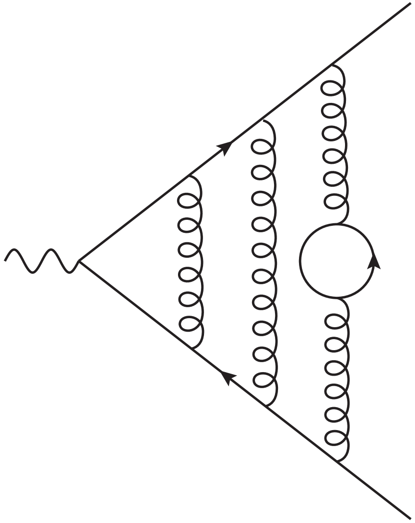
$n_{f}C_{F}^{3}$

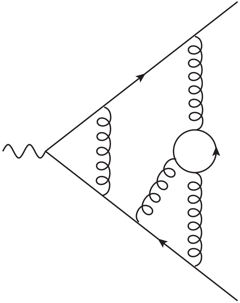
$n_{f}C_{F}^{2}C_{A}$

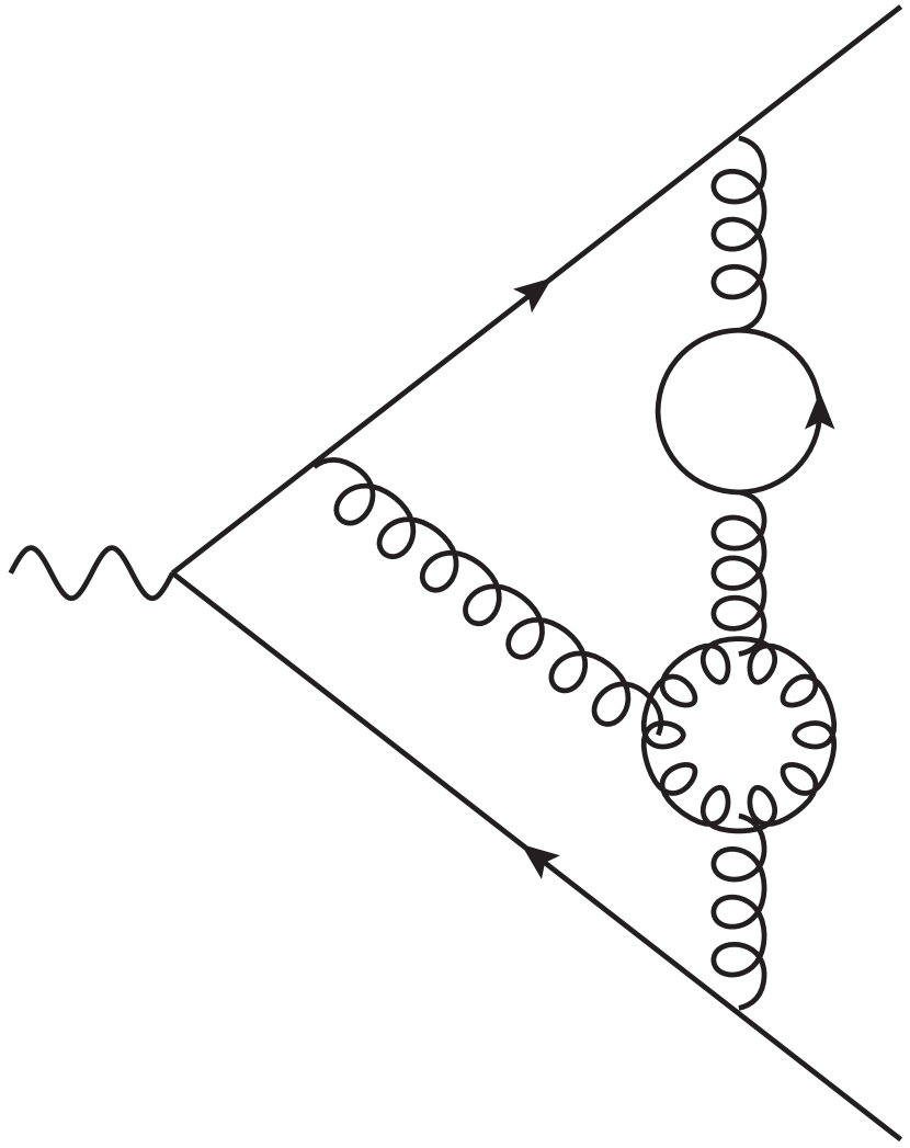
$n_{f}C_{F}C_{A}^{2}$

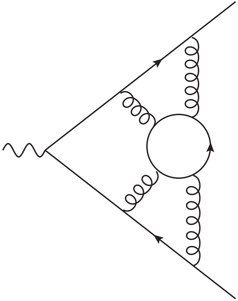
$n_{f}(d^{abcd}_{F})^{2}$

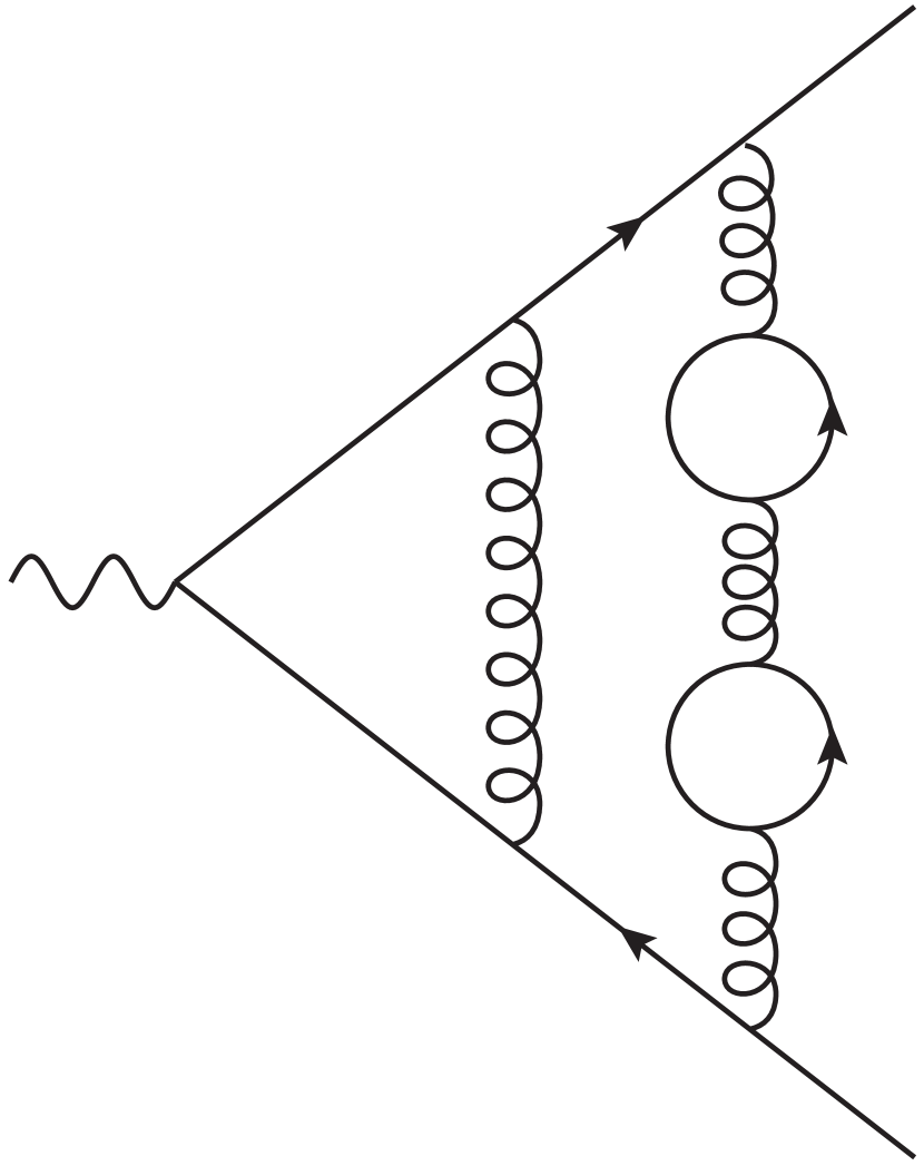
$n_{f}^{2}C_{F}^{2}$

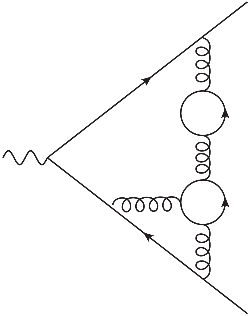
$n_{f}^{2}C_{F}C_{A}$

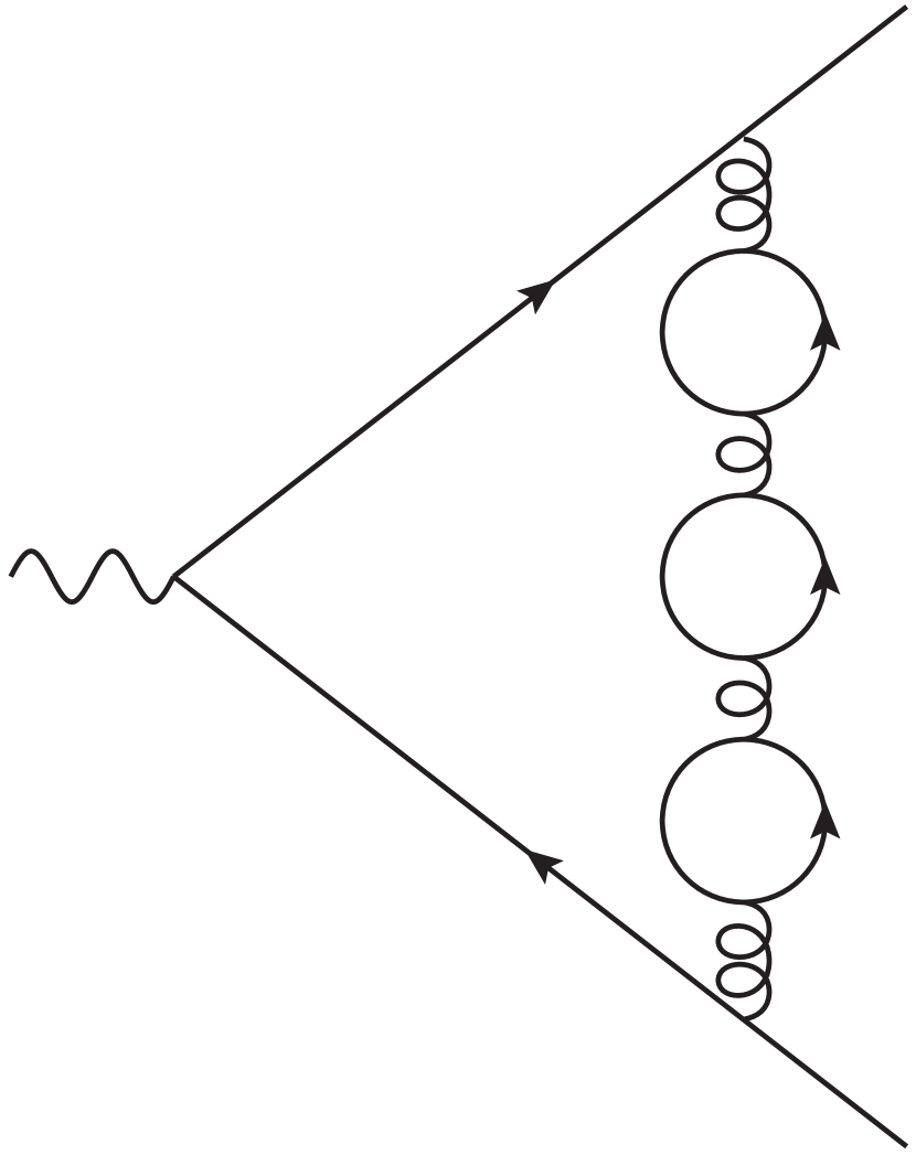
$n_{f}^{3}C_{F}$

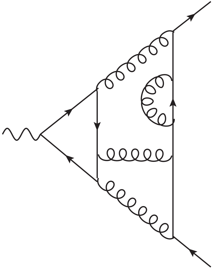
$n_{q\gamma}(d^{abc}_{F})^{2}C_{F}$

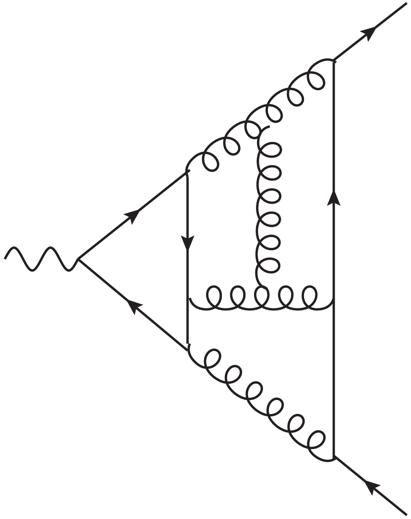
$n_{q\gamma}(d^{abc}_{F})^{2}C_{A}$

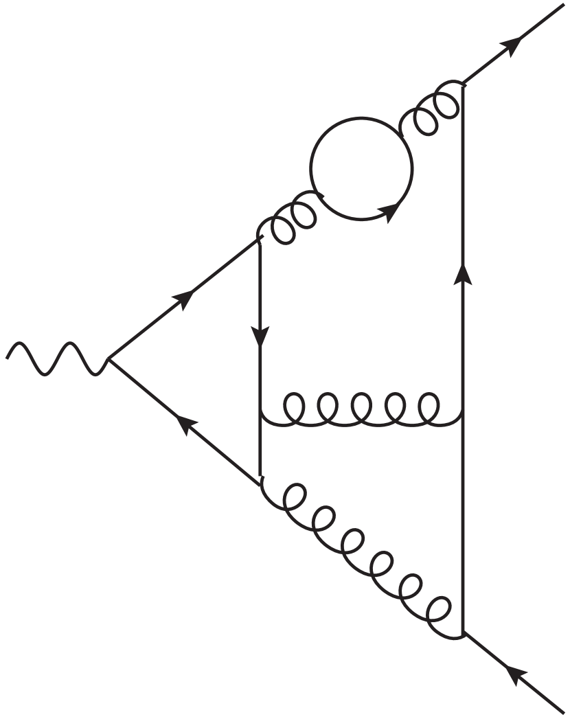
$n_{q\gamma}n_{f}(d^{abc}_{F})^{2}$

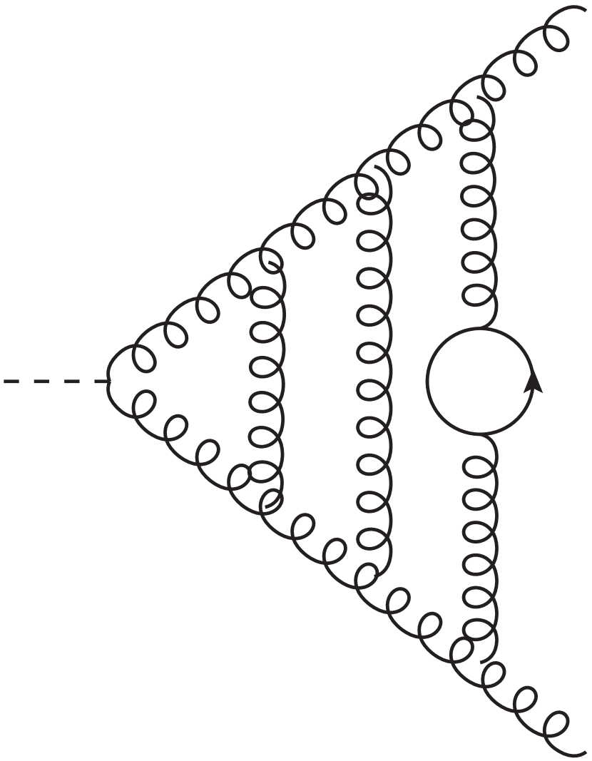
$n_{f}C_{A}^{3}$

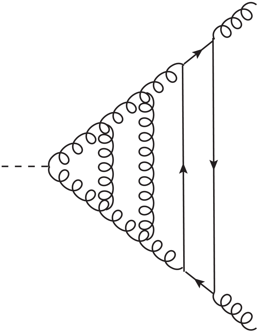
$n_{f}C_{A}^{2}C_{F}$

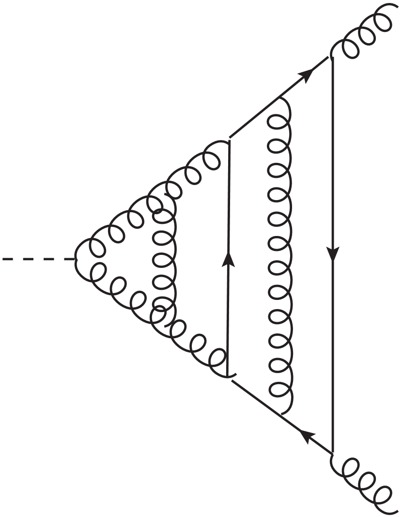
$n_{f}C_{A}C_{F}^{2}$

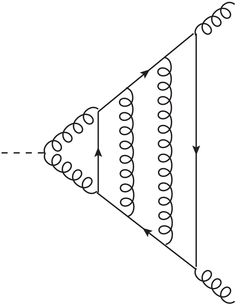
$n_{f}C_{F}^{3}$

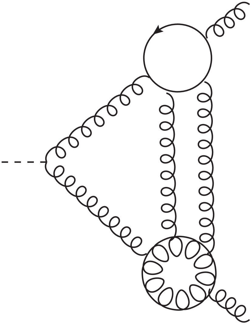
$n_{f}d_{A}^{abcd}d_{F}^{abcd}$

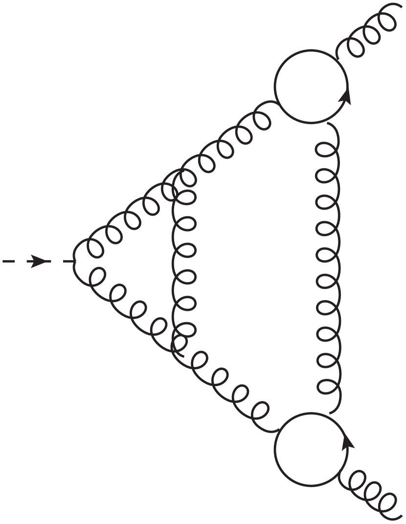
$n_{f}^{2}C_{A}^{2}$

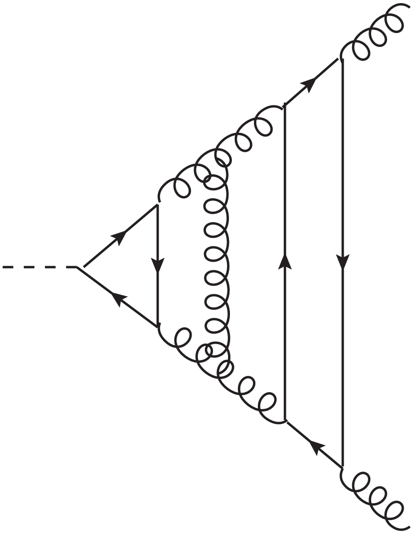
$n_{f}^{2}C_{A}C_{F}$

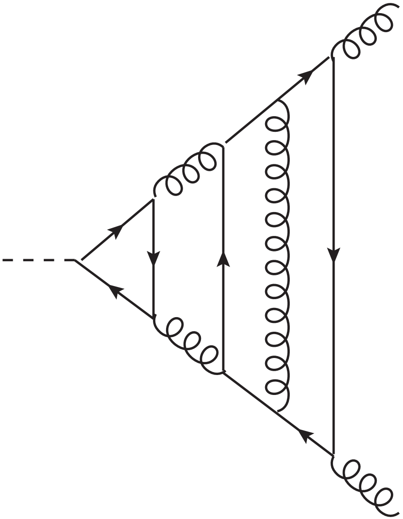
$n_{f}^{2}C_{A}C_{F}^{2}$

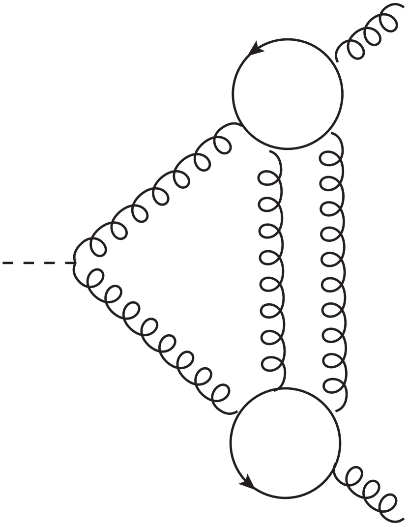
$n_{f}^{2}(d_{F}^{abcd})^{2}$

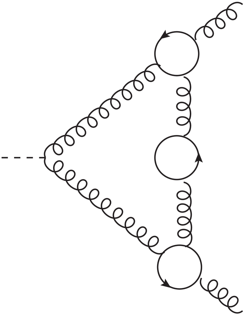
$n_{f}^{3}C_{A}$

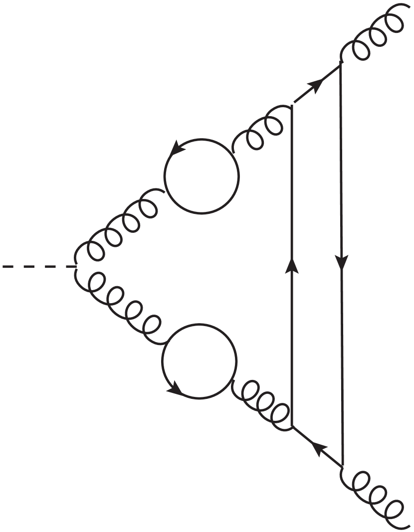
$n_{f}^{3}C_{F}$

Figure 1: Sample Feynman diagrams contributing to the fermionic corrections to $F_{q}$ and $F_{g}$ at four-loop order. Straight and curly lines denote quarks and gluons, respectively. Both planar and non-planar diagrams contribute.

We define the perturbative expansion of $F_{q}$ and $F_{g}$ in terms of the bare strong coupling constant and write

$$F_{x} = 1+\sum_{n\geq 1}\left(\frac{\alpha_{s}^{0}}{4\pi}\right)^{n}\left(\frac{4\pi}{e^{\gamma_{E}}}\right)^{n\epsilon}\left(\frac{\mu^{2}}{-q^{2}-i0}\right)^{n\epsilon}F_{x}^{(n)}\,,$$

with $x\in\{q,g\}$.

Two-loop corrections to $F_{q}$ have been computed in Refs. [4, 5, 6, 7] and the first two-loop calculation for $F_{g}$ has been performed in [8]. In the first three-loop calculation of $F_{q}$ and $F_{g}$ [9] the coefficients of the highest $\epsilon$ expansion terms of three master integrals were only known numerically. These coefficients have been computed in [10]. The results of [9] have been confirmed in Refs. [11, 12, 13]. For the computation of three-loop master integrals we also refer to [14].

At four-loop order there are only partial results. For $F_{q}$, the large-$N_{c}$ limit, which only involves planar diagrams, has been considered in Refs. [15, 16], the $n_{f}^{2}$ terms are available from [17], the complete contribution from color structure $(d_{F}^{abcd})^{2}$ has been computed in [18] and confirmed in [19]. For $F_{q}$ and $F_{g}$, all corrections with three or two closed fermion loops were calculated in [20, 21], respectively, including also the singlet contributions.

There are a number of works where pole parts of the form factors have been computed. In fact, from the $1/\epsilon^{2}$ pole it is possible to extract the so-called cusp anomalous dimension. A complete calculation based on the form factors can be found in Ref. [19]. In that work a basis of finite integrals has been chosen and expanded only to lower orders in $\epsilon$ in order to obtain the required weight six information. Ref. [19] confirmed the expression presented in Ref. [22], which is based on a calculation in $\mathcal{N}=4$ super Yang-Mills, other known QCD results, and conjectural input for one term in the matter contributions. Partial contributions to the QCD cusp anomalous dimension are available from [23, 24, 20, 15, 16, 17, 25, 26] and numerical results are presented in Refs. [27, 28].

Recently, the collinear anomalous dimensions of the quark and gluon form factors have been computed in Ref. [29] by extracting the $1/\epsilon$ poles of the corresponding form factors. All contributions could be computed analytically except one contribution from a non-planar four-loop integral defined in $6-2\epsilon$ dimensions, which is parameterized by ${\cal H}$ (c.f. Eq. (10) of [29]),

$$\mathrel{\mathop{\vbox{\hbox{\includegraphics[scale={.15}]{D_12_27631H}}}}\limits^{\vbox to-1.80835pt{\kern-2.0pt\hbox{$\scriptstyle{(6-2\epsilon)\qquad}$}\vss}}}\equiv\mathcal{H}+{\mathcal{O}\left(\epsilon\right)}.$$ (3)

Using a numerical evaluation of ${\cal H}$ to 10 significant digits together with an assumption on the multiple zeta values present in ${\cal H}$, an analytic expression could be conjectured. Using the results obtained in the present paper we confirm this expression; details are presented in the next Section where we outline some of the techniques used for our calculation. Our analytic results are presented in Section III and Section IV contains our conclusions and an outlook to the full result.

II Calculation

We employ Qgraf [30] to generate the required Feynman diagrams with closed fermion loops, 2464 diagrams for $F_{q}^{(4)}$ and 18642 diagrams for $F_{g}^{(4)}$. After applying the projectors and performing the numerator algebra with Form 4 [31], we obtain the form factors $F_{q}$ and $F_{g}$ expressed as a linear combination of scalar functions belonging to properly defined integral families. Each function has 18 indices where up to twelve correspond to the different propagators of the diagrams. In addition to planar diagrams (see, e.g., Ref. [15, 16, 32]) there are non-planar diagrams; it is the latter which pose challenges. We perform the calculation in a general $R_{\xi}$ gauge and check explicitly that terms proportional to $\xi$ cancel in our results.

From the computational point of view there are two challenges one has to deal with. The first one is the integration-by-parts reduction [33, 34] of the scalar integrals, which appear in the amplitudes, to so-called master integrals. For this task, we employ the setup described in Ref. [19], which is based on the codes Reduze 2 [35] and Finred, implementing techniques from [36, 37, 38, 39, 40, 41, 42].

The second challenge is the computation of the master integrals as a Laurent series in $\epsilon$. Here we have two approaches at hand. The first one is based on the construction of a basis of finite master integrals [43, 13, 44], partly in $6-2\epsilon$ dimensions. Subsequently the program HyperInt [45] is used to compute the $\epsilon$ expansion of the master integrals. This approach allowed us to compute all $\epsilon$ coefficients of the master integrals required for the fermionic four-loop corrections except for $\mathcal{H}$. We wish to note, however, that it remains unclear whether the evaluation of the constants of transcendental weight eight (or even higher) of some of the non-planar twelve-line master integrals is possible in this approach. In particular, for the two Feynman integrals corresponding to non-planar graphs with twelve edges

       (4)

it is not known whether a linearly reducible [46, 47] Feynman parametric representation exists.

In this Letter, we show that both remaining non-linearly reducible topologies (4) can be solved using a second method, which is based on differential equations. While the method of differential equations [48, 49, 50] is not directly applicable to one-scale Feynman integrals, we can introduce an additional scale parameter, as was suggested in Ref. [51]. On the one hand, we complicate the situation. On the other hand, we obtain the possibility to apply the full power of the method of differential equations (see, e.g., Refs. [52, 53] and Ref. [54, Section E.8]). In the context of massless four-loop form factors this approach has been applied successfully in Refs. [15, 16, 17, 18]. In a first step one introduces a second mass scale by imposing a virtuality $q_{2}^{2}\not=0$ on one of the external partons, which apparently makes the problem more complicated. However, we are now in a position to establish differential equations for the master integrals in the variable $x=q_{2}^{2}/q^{2}$ which determine the connection between the points $x=1$ and $x=0$. The boundary conditions are then easy to fix at $x=1$ as in this point our integrals turn into massless propagator integrals for which analytic results are known at least up to weight twelve [55, 56]. A detailed description of the procedure can be found in Ref. [18].

In our calculation we employ Fire 6 [57] in combination with LiteRed [40, 58] to compute the reductions for the differential equations and closely follow the algorithm of Refs. [59, 60] as implemented in Libra [61] to bring our system in $\epsilon$-form. The complexity of the two topologies (4) is somewhat reflected also in the properties of the differential equations. First, it appears that differential equations for these two topologies, in addition to singularities at $x=0$ and $1$, have singularities at $x=-1,\,4,\,1/4$ (at $x=4$) for the first (second) topology, respectively. Among those, the singularity at $x=1/4$ is especially troublesome as it lies inside the segment $(0,1)$ connecting the points of interest. Moreover, it appears that in order to reduce the system to $\epsilon$-form, we need to introduce the algebraic extensions $x_{1}=\sqrt{x}$, $x_{2}=\sqrt{x-1/4}$, and $x_{3}=\sqrt{1/x-1/4}$. Fortunately, for each specific iterated integral which appears in the $\epsilon$ expansion of the master integrals of these two topologies it is possible to find the rationalizing variable change. As a result, the master integrals of the two topologies are not directly expressed via non-alternating multiple zeta values, but rather via Goncharov polylogarithms with letters in the alphabet $\{0,\pm 1,\pm i\sqrt{3},e^{\pm i\pi/3},e^{\pm 2i\pi/3},e^{\pm i\pi/3}/2\}$. Using the PSLQ algorithm, we were able to express our final result for the master integrals with two massless legs and their subtopologies through to weight nine in terms of regular zeta values, $\zeta_{n}$ $(n=2,\ldots,9)$, and the multiple zeta value

$$\zeta_{5,3}=\sum_{m=1}^{\infty}\sum_{n=1}^{m-1}\frac{1}{m^{5}n^{3}}\approx 0.0377076729848\,.$$ (5)

Our results for the corner integrals of the two non-planar topologies through to the finite parts are

$$\vbox{\hbox{\includegraphics[scale={.15}]{D_12_27631}}}=\frac{1}{\epsilon^{8}}\Big{(}\mfrac{7}{18}\Big{)}+\frac{1}{\epsilon^{7}}\Big{(}\mfrac{55}{24}\Big{)}+\frac{1}{\epsilon^{6}}\Big{(}-\mfrac{67}{9}\zeta_{2}-\mfrac{797}{144}\Big{)}+\frac{1}{\epsilon^{5}}\Big{(}-\mfrac{442}{9}\zeta_{3}-\mfrac{643}{18}\zeta_{2}+\mfrac{1193}{144}\Big{)}+\frac{1}{\epsilon^{4}}\Big{(}-\mfrac{9199}{360}\zeta_{2}^{2}-\mfrac{3547}{18}\zeta$$

$$\qquad+\mfrac{7793}{72}\zeta_{2}+\mfrac{1013}{48}\Big{)}+\frac{1}{\epsilon^{3}}\Big{(}-\mfrac{2858}{3}\zeta_{5}+\mfrac{27617}{36}\zeta_{3}\zeta_{2}-\mfrac{3439}{180}\zeta_{2}^{2}+\mfrac{60893}{72}\zeta_{3}-\mfrac{1897}{8}\zeta_{2}-\mfrac{43895}{144}\Big{)}+\frac{1}{\epsilon^{2}}\Big{(}\mfrac{179927}{72}\zeta_{3}^{2}-\mfrac{40853}{252}\zeta_{2}^{3}$$

$$\qquad-\scalebox{0.85}{2780}\zeta_{5}+\mfrac{23467}{9}\zeta_{3}\zeta_{2}+\mfrac{132359}{180}\zeta_{2}^{2}-\mfrac{66607}{24}\zeta_{3}-\mfrac{5423}{72}\zeta_{2}+\mfrac{311383}{144}\Big{)}+\frac{1}{\epsilon}\Big{(}-\mfrac{1015395}{32}\zeta_{7}+\mfrac{30493}{2}\zeta_{5}\zeta_{2}+\mfrac{274199}{90}\zeta_{3}\zeta_{2}^{2}$$

$$\qquad+\mfrac{44984}{9}\zeta_{3}^{2}-\mfrac{540823}{420}\zeta_{2}^{3}+\mfrac{477281}{24}\zeta_{5}-\mfrac{412181}{36}\zeta_{3}\zeta_{2}-\mfrac{117101}{30}\zeta_{2}^{2}+\mfrac{410629}{72}\zeta_{3}+\mfrac{400999}{72}\zeta_{2}-\mfrac{622069}{48}\Big{)}+\mfrac{122261}{15}\zeta_{5,3}$$

$$\qquad+\mfrac{1298525}{12}\zeta_{5}\zeta_{3}-\mfrac{942899}{36}\zeta_{3}^{2}\zeta_{2}-\mfrac{121150681}{9000}\zeta_{2}^{4}-\mfrac{2558101}{16}\zeta_{7}+\mfrac{360793}{6}\zeta_{5}\zeta_{2}-\mfrac{53821}{18}\zeta_{3}\zeta_{2}^{2}-\mfrac{1428953}{72}\zeta_{3}^{2}+\mfrac{2037031}{168}\zeta_{2}^{3}$$

$$\qquad-\mfrac{1989461}{24}\zeta_{5}+\mfrac{526387}{12}\zeta_{3}\zeta_{2}+\mfrac{245017}{18}\zeta_{2}^{2}+\mfrac{738547}{72}\zeta_{3}-\mfrac{1198061}{24}\zeta_{2}+\mfrac{10519199}{144}+\mathcal{O}(\epsilon),$$ (6)

$$\vbox{\hbox{\includegraphics[scale={.15}]{E_12_47063}}}=\frac{1}{\epsilon^{8}}\Big{(}\mfrac{1}{18}\Big{)}+\frac{1}{\epsilon^{7}}\Big{(}\mfrac{13}{48}\Big{)}+\frac{1}{\epsilon^{6}}\Big{(}-\mfrac{4}{9}\zeta_{2}-\mfrac{193}{192}\Big{)}+\frac{1}{\epsilon^{5}}\Big{(}-\mfrac{395}{72}\zeta_{3}-\mfrac{175}{144}\zeta_{2}+\mfrac{167}{48}\Big{)}+\frac{1}{\epsilon^{4}}\Big{(}-\mfrac{13577}{720}\zeta_{2}^{2}-\mfrac{347}{18}\zeta_{3}$$

$$\qquad+\mfrac{373}{96}\zeta_{2}-\mfrac{385}{36}\Big{)}+\frac{1}{\epsilon^{3}}\Big{(}-\mfrac{5941}{24}\zeta_{5}-\mfrac{799}{36}\zeta_{3}\zeta_{2}-\mfrac{130661}{1440}\zeta_{2}^{2}+\mfrac{1043}{32}\zeta_{3}-\mfrac{1225}{72}\zeta_{2}+\mfrac{1771}{72}\Big{)}+\frac{1}{\epsilon^{2}}\Big{(}-\mfrac{1687}{72}\zeta_{3}^{2}-\mfrac{1495399}{5040}\zeta_{2}^{3}$$

$$\qquad-\mfrac{23419}{24}\zeta_{5}-\mfrac{6953}{24}\zeta_{3}\zeta_{2}+\mfrac{13921}{90}\zeta_{2}^{2}-\mfrac{6655}{72}\zeta_{3}+\mfrac{730}{9}\zeta_{2}+\mfrac{11}{4}\Big{)}+\frac{1}{\epsilon^{1}}\Big{(}-\mfrac{433869}{64}\zeta_{7}-\mfrac{21667}{24}\zeta_{5}\zeta_{2}+\mfrac{101723}{90}\zeta_{3}\zeta_{2}^{2}-\mfrac{5267}{12}\zeta_{3}^{2}$$

$$\qquad-\mfrac{14629019}{10080}\zeta_{2}^{3}+\mfrac{257675}{96}\zeta_{5}+\mfrac{30845}{144}\zeta_{3}\zeta_{2}-\mfrac{981}{8}\zeta_{2}^{2}+\mfrac{45509}{72}\zeta_{3}-\mfrac{8633}{24}\zeta_{2}-\mfrac{41461}{72}\Big{)}+\mfrac{43916}{15}\zeta_{5,3}+\mfrac{44957}{4}\zeta_{5}\zeta_{3}$$

$$\qquad+\mfrac{133033}{36}\zeta_{3}^{2}\zeta_{2}-\mfrac{257784979}{56000}\zeta_{2}^{4}-\mfrac{1611457}{64}\zeta_{7}-\mfrac{207481}{24}\zeta_{5}\zeta_{2}+\mfrac{4033391}{720}\zeta_{3}\zeta_{2}^{2}+\mfrac{846605}{288}\zeta_{3}^{2}+\mfrac{4194707}{1440}\zeta_{2}^{3}-\mfrac{76189}{12}\zeta_{5}$$

$$\qquad+\mfrac{61787}{36}\zeta_{3}\zeta_{2}-\mfrac{168493}{360}\zeta_{2}^{2}-\mfrac{59869}{12}\zeta_{3}+\mfrac{48311}{36}\zeta_{2}+\mfrac{197863}{36}+\mathcal{O}(\epsilon)$$ (7)

in the conventions of [32]. Combining the integral solutions obtained by direct integration with the result (II) allows us to determine

$$\mathcal{H} =\mfrac{161}{16}\zeta_{7}+\mfrac{5}{2}\zeta_{5}\zeta_{2}-\frac{5}{2}\zeta_{3}\zeta_{2}^{2}+\scalebox{0.85}{10}\zeta_{3}^{2}+\mfrac{223}{210}\zeta_{2}^{3}-\scalebox{0.85}{25}\zeta_{5}$$

$$\quad-\scalebox{0.85}{6}\zeta_{3}\zeta_{2}+\mfrac{3}{10}\zeta_{2}^{2}+\scalebox{0.85}{9}\zeta_{3}\,.$$ (8)

This value for $\mathcal{H}$ agrees with the expression conjectured in [29] and thus confirms the non-fermionic contributions to the collinear anomalous dimensions in that reference analytically. Moreover, this result provides the last remaining master integral coefficient required for the present calculation.

III Results for form factors

In this Section we present the complete fermionic four-loop corrections to the form factors $F_{q}$ and $F_{g}$ in massless QCD. We express the results in terms of $SU(N_{c})$ color factors and use

$$C_{F}=\frac{N_{c}^{2}-1}{2N_{c}}\,,\quad C_{A}=N_{c}\,,\quad N_{A}=N_{c}^{2}-1\,,$$

$$N_{F}=N_{c}\,,\quad n_{q\gamma}=\sum_{q^{\prime}}\frac{Q_{q^{\prime}}}{Q_{q}}\,,\quad\frac{d_{F}^{abc}d_{F}^{abc}}{N_{A}}=\frac{N_{c}^{2}-4}{16N_{c}}\,,$$

$$\frac{d_{F}^{abcd}d_{F}^{abcd}}{N_{A}}=\frac{N_{c}^{4}-6N_{c}^{2}+18}{96N_{c}^{2}}\,,$$

$$\frac{d_{A}^{abcd}d_{F}^{abcd}}{N_{A}}=\frac{N_{c}(N_{c}^{2}+6)}{48}\,,$$ (9)

where $Q_{q}$ is the fractional charge of the quark $q$ and $n_{f}$ is the number of active quark flavors. Without loss of generality we have used for the trace normalization $T_{F}=1/2$.

The $\epsilon$ expansion of the fermionic corrections to both form factors start with seventh order poles in $1/\epsilon$, reflecting the fact that fermionic corrections start to contribute only at two loops. Similarly, four-loop contributions with more than two closed fermion loops or specific color factors start even later in the $\epsilon$ expansion. The corresponding poles through to order $1/\epsilon$ can be obtained from [19]; they consist of zeta values with transcendental weight up to six.

Here, we calculate the complete finite part of the fermionic four-loop contributions to $F_{q}$ and $F_{g}$ and obtain an analytical result in terms of zeta values with transcendental weight up to seven. Our result for the finite part of $F_{q}^{(4)}$ reads

$$\left.F_{q}^{(4)}\right|_{\epsilon^{0}} ={\color[rgb]{0.0,0.0,0.7}n_{f}C_{F}^{3}}\Big{(}\mfrac{1153615}{126}\zeta_{7}+\mfrac{6316}{9}\zeta_{5}\zeta_{2}+\mfrac{229468}{135}\zeta_{3}\zeta_{2}^{2}+\mfrac{547270}{81}\zeta_{3}^{2}+\mfrac{1341628}{2835}\zeta_{2}^{3}-\mfrac{3467995}{162}\zeta_{5}-\mfrac{192737}{81}\zeta_{3}\zeta_{2}-\mfrac{1420133}{1215}\zeta_{2}^{2}$$

$$-\mfrac{38482147}{972}\zeta_{3}+\mfrac{12734681}{648}\zeta_{2}+\mfrac{7837713013}{419904}\Big{)}+{\color[rgb]{0.0,0.0,0.7}n_{f}C_{A}C_{F}^{2}}\Big{(}\mfrac{5669}{4}\zeta_{7}-\mfrac{249194}{135}\zeta_{5}\zeta_{2}-\mfrac{417244}{405}\zeta_{3}\zeta_{2}^{2}-\mfrac{11438080}{729}\zeta_{3}^{2}$$

$$-\mfrac{38510}{63}\zeta_{2}^{3}+\mfrac{4959127}{243}\zeta_{5}+\mfrac{408107}{81}\zeta_{3}\zeta_{2}+\mfrac{8388679}{2916}\zeta_{2}^{2}+\mfrac{2642551543}{26244}\zeta_{3}-\mfrac{111491363}{2187}\zeta_{2}-\mfrac{326984889779}{3779136}\Big{)}$$

$$+{\color[rgb]{0.0,0.0,0.7}n_{f}C_{A}^{2}C_{F}}\Big{(}\mfrac{6943}{24}\zeta_{7}+\mfrac{2755}{9}\zeta_{5}\zeta_{2}+\mfrac{1912}{45}\zeta_{3}\zeta_{2}^{2}+\mfrac{202210}{27}\zeta_{3}^{2}+\mfrac{128953}{1620}\zeta_{2}^{3}-\mfrac{34844257}{3240}\zeta_{5}-\mfrac{119489}{108}\zeta_{3}\zeta_{2}-\mfrac{1251893}{540}\zeta_{2}^{2}$$

$$-\mfrac{111467677}{1944}\zeta_{3}+\mfrac{123861583}{3888}\zeta_{2}+\mfrac{21075909203}{279936}\Big{)}+{\color[rgb]{0.0,0.0,0.7}n_{f}\mfrac{d_{F}^{abcd}d_{F}^{abcd}}{N_{F}}}\Big{(}-\scalebox{0.85}{1240}\zeta_{7}+\mfrac{992}{3}\zeta_{5}\zeta_{2}-\mfrac{3952}{15}\zeta_{3}\zeta_{2}^{2}+\mfrac{680}{9}\zeta_{3}^{2}+\mfrac{41620}{189}\zeta_{2}^{3}$$

$$+\mfrac{95098}{27}\zeta_{5}+\mfrac{92}{3}\zeta_{3}\zeta_{2}+\mfrac{7552}{45}\zeta_{2}^{2}-\mfrac{21566}{9}\zeta_{2}-\mfrac{13414}{27}\zeta_{3}+\mfrac{3190}{3}\Big{)}+{\color[rgb]{0.0,0.0,0.7}n_{f}^{2}C_{F}^{2}}\Big{(}\mfrac{689582}{729}\zeta_{3}^{2}+\mfrac{191252}{945}\zeta_{2}^{3}+\mfrac{187364}{1215}\zeta_{5}$$

$$+\mfrac{177800}{729}\zeta_{3}\zeta_{2}+\mfrac{4777}{135}\zeta_{2}^{2}-\mfrac{90719803}{13122}\zeta_{3}+\mfrac{44208841}{13122}\zeta_{2}+\mfrac{5325319081}{944784}\Big{)}+{\color[rgb]{0.0,0.0,0.7}n_{f}^{2}C_{A}C_{F}}\Big{(}-\mfrac{1714}{3}\zeta_{3}^{2}-\mfrac{2836}{315}\zeta_{2}^{3}+\mfrac{150886}{135}\zeta_{5}$$

$$-\mfrac{436}{3}\zeta_{3}\zeta_{2}-\mfrac{3722}{135}\zeta_{2}^{2}+\mfrac{2897315}{486}\zeta_{3}-\mfrac{5825827}{1296}\zeta_{2}-\mfrac{3325501813}{279936}\Big{)}+{\color[rgb]{0.0,0.0,0.7}n_{f}^{3}C_{F}}\Big{(}-\mfrac{2194}{135}\zeta_{5}-\mfrac{820}{81}\zeta_{3}\zeta_{2}+\mfrac{3322}{135}\zeta_{2}^{2}-\mfrac{20828}{243}\zeta_{3}$$

$$+\mfrac{145115}{729}\zeta_{2}+\mfrac{10739263}{17496}\Big{)}+{\color[rgb]{0.0,0.0,0.7}n_{q\gamma}\mfrac{d_{F}^{abc}d_{F}^{abc}C_{F}}{N_{F}}}\Big{(}\scalebox{0.85}{26624}\zeta_{7}+\scalebox{0.85}{1792}\zeta_{5}\zeta_{2}+\mfrac{35584}{15}\zeta_{3}\zeta_{2}^{2}+\mfrac{30688}{9}\zeta_{3}^{2}-\mfrac{179152}{189}\zeta_{2}^{3}-\mfrac{170224}{27}\zeta_{5}$$

$$-\mfrac{8656}{3}\zeta_{3}\zeta_{2}+\mfrac{60416}{45}\zeta_{2}^{2}-\mfrac{100624}{9}\zeta_{2}-\mfrac{71552}{27}\zeta_{3}-\mfrac{89360}{9}\Big{)}+{\color[rgb]{0.0,0.0,0.7}n_{q\gamma}\mfrac{d_{F}^{abc}d_{F}^{abc}C_{A}}{N_{F}}}\Big{(}-\mfrac{13972}{3}\zeta_{7}-\scalebox{0.85}{1840}\zeta_{5}\zeta_{2}-\mfrac{784}{5}\zeta_{3}\zeta_{2}^{2}$$

$$-\scalebox{0.85}{13008}\zeta_{3}^{2}-\mfrac{618328}{189}\zeta_{2}^{3}+\mfrac{54436}{9}\zeta_{5}+\mfrac{15112}{3}\zeta_{3}\zeta_{2}-\mfrac{95692}{45}\zeta_{2}^{2}+\mfrac{45976}{9}\zeta_{3}+\mfrac{107984}{9}\zeta_{2}+\mfrac{65264}{9}\Big{)}+{\color[rgb]{0.0,0.0,0.7}n_{q\gamma}n_{f}\mfrac{d_{F}^{abc}d_{F}^{abc}}{N_{F}}}\Big{(}\scalebox{0.85}{2304}\zeta_{3}^{2}$$

$$+\mfrac{545792}{945}\zeta_{2}^{3}-\mfrac{8512}{9}\zeta_{5}-\mfrac{1888}{3}\zeta_{3}\zeta_{2}+\mfrac{12448}{45}\zeta_{2}^{2}-\mfrac{3520}{9}\zeta_{3}-\mfrac{16928}{9}\zeta_{2}-\mfrac{11296}{9}\Big{)}$$

$$+\text{contributions without closed fermion loop}.$$ (10)

For the finite part of $F_{g}^{(4)}$ we obtain

$$\left.F_{g}^{(4)}\right|_{\epsilon^{0}} ={\color[rgb]{0.0,0.0,0.7}n_{f}C_{A}^{3}}\Big{(}\mfrac{365579}{63}\zeta_{7}-\mfrac{64151}{135}\zeta_{5}\zeta_{2}+\mfrac{410228}{405}\zeta_{3}\zeta_{2}^{2}-\mfrac{11278261}{2916}\zeta_{3}^{2}-\mfrac{1672838}{2835}\zeta_{2}^{3}-\mfrac{24219919}{4860}\zeta_{5}+\mfrac{638345}{486}\zeta_{3}\zeta_{2}$$

$$-\mfrac{1464209}{29160}\zeta_{2}^{2}+\mfrac{483257171}{52488}\zeta_{3}-\mfrac{55297501}{34992}\zeta_{2}-\mfrac{322439904151}{7558272}\Big{)}+{\color[rgb]{0.0,0.0,0.7}n_{f}C_{A}^{2}C_{F}}\Big{(}-\mfrac{66967}{36}\zeta_{7}+\mfrac{10022}{9}\zeta_{5}\zeta_{2}-\mfrac{8824}{9}\zeta_{3}\zeta_{2}^{2}$$

$$+\mfrac{129887}{81}\zeta_{3}^{2}-\mfrac{163538}{945}\zeta_{2}^{3}+\mfrac{2166853}{1620}\zeta_{5}+\mfrac{91172}{81}\zeta_{3}\zeta_{2}-\mfrac{10414}{27}\zeta_{2}^{2}+\mfrac{25799269}{5832}\zeta_{3}-\mfrac{6154445}{3888}\zeta_{2}-\mfrac{821501405}{139968}\Big{)}$$

$$+{\color[rgb]{0.0,0.0,0.7}n_{f}C_{A}C_{F}^{2}}\Big{(}\scalebox{0.85}{2692}\zeta_{7}-\scalebox{0.85}{1420}\zeta_{5}\zeta_{2}+\mfrac{2500}{3}\zeta_{3}\zeta_{2}^{2}+\mfrac{2720}{3}\zeta_{3}^{2}+\mfrac{376624}{945}\zeta_{2}^{3}-\mfrac{50591}{6}\zeta_{5}+\mfrac{1321}{3}\zeta_{3}\zeta_{2}-\mfrac{4057}{5}\zeta_{2}^{2}+\mfrac{85357}{36}\zeta_{3}$$

$$+\mfrac{6451}{36}\zeta_{2}-\mfrac{24275}{432}\Big{)}+{\color[rgb]{0.0,0.0,0.7}n_{f}C_{F}^{3}}\Big{(}\scalebox{0.85}{3360}\zeta_{7}-\scalebox{0.85}{2940}\zeta_{5}-\scalebox{0.85}{156}\zeta_{3}+\mfrac{169}{2}\Big{)}+{\color[rgb]{0.0,0.0,0.7}n_{f}\mfrac{d_{A}^{abcd}d_{F}^{abcd}}{N_{A}}}\Big{(}\mfrac{2464}{3}\zeta_{7}+\scalebox{0.85}{1824}\zeta_{5}\zeta_{2}-\mfrac{1088}{3}\zeta_{3}\zeta_{2}^{2}$$

$$-\mfrac{15700}{3}\zeta_{3}^{2}-\mfrac{245536}{945}\zeta_{2}^{3}+\mfrac{108692}{9}\zeta_{5}+\mfrac{1544}{9}\zeta_{3}\zeta_{2}-\mfrac{35108}{45}\zeta_{2}^{2}-\mfrac{89932}{9}\zeta_{3}+\mfrac{9580}{27}\zeta_{2}+\mfrac{6944}{9}\Big{)}+{\color[rgb]{0.0,0.0,0.7}n_{f}^{2}C_{A}^{2}}\Big{(}\mfrac{717266}{729}\zeta_{3}^{2}$$

$$+\mfrac{58858}{945}\zeta_{2}^{3}-\mfrac{62671}{1215}\zeta_{5}-\mfrac{87329}{1458}\zeta_{3}\zeta_{2}+\mfrac{380701}{3240}\zeta_{2}^{2}+\mfrac{27036815}{52488}\zeta_{3}-\mfrac{53253361}{104976}\zeta_{2}+\mfrac{110016540845}{7558272}\Big{)}+{\color[rgb]{0.0,0.0,0.7}n_{f}^{2}C_{A}C_{F}}\Big{(}\!-\mfrac{4354}{3}\zeta_{3}^{2}$$

$$-\mfrac{143524}{945}\zeta_{2}^{3}-\mfrac{47948}{27}\zeta_{5}-\mfrac{3688}{9}\zeta_{3}\zeta_{2}-\mfrac{13820}{81}\zeta_{2}^{2}-\mfrac{538853}{162}\zeta_{3}-\mfrac{27629}{81}\zeta_{2}+\mfrac{3697777}{324}\Big{)}+{\color[rgb]{0.0,0.0,0.7}n_{f}^{2}C_{F}^{2}}\Big{(}\mfrac{2432}{3}\zeta_{3}^{2}+\mfrac{32512}{135}\zeta_{2}^{3}$$

$$+\scalebox{0.85}{3360}\zeta_{5}+\mfrac{128}{3}\zeta_{3}\zeta_{2}-\mfrac{484}{3}\zeta_{2}^{2}-\mfrac{36260}{9}\zeta_{3}+\mfrac{439}{9}\zeta_{2}-\mfrac{80281}{216}\Big{)}+{\color[rgb]{0.0,0.0,0.7}n_{f}^{2}\mfrac{d_{F}^{abcd}d_{F}^{abcd}}{N_{A}}}\Big{(}\scalebox{0.85}{512}\zeta_{3}^{2}-\scalebox{0.85}{960}\zeta_{5}+\mfrac{384}{5}\zeta_{2}^{2}+\scalebox{0.85}{1520}\zeta_{3}$$

$$-\mfrac{9008}{9}\Big{)}+{\color[rgb]{0.0,0.0,0.7}n_{f}^{3}C_{A}}\Big{(}-\mfrac{14474}{135}\zeta_{5}+\mfrac{4556}{81}\zeta_{3}\zeta_{2}-\mfrac{1418}{27}\zeta_{2}^{2}-\mfrac{99890}{243}\zeta_{3}+\mfrac{38489}{729}\zeta_{2}-\mfrac{20832641}{17496}\Big{)}+{\color[rgb]{0.0,0.0,0.7}n_{f}^{3}C_{F}}\Big{(}-\mfrac{508069}{324}$$

$$+\mfrac{4288}{27}\zeta_{5}-\scalebox{0.85}{64}\zeta_{3}\zeta_{2}+\mfrac{2288}{27}\zeta_{2}^{2}+\mfrac{24812}{27}\zeta_{3}+\mfrac{3074}{27}\zeta_{2}\Big{)}$$

$$+\text{contributions without closed fermion loop}.$$ (11)

The $n_{f}^{3}$, $n_{f}^{2}$ and $n_{q\gamma}n_{f}$ terms agree with the results presented in Refs. [20, 21]. Our expression for $F_{q}$ reproduces the result of Ref. [15] in the large-$N_{c}$ limit. The remaining, subleading color terms for $F_{q}^{(4)}$ and all of the terms linear in $n_{f}$ for $F_{g}^{(4)}$ are new.

IV Conclusions

In this Letter, we calculated the complete fermionic corrections to the photon-quark and Higgs-gluon vertices in massless four-loop QCD. We solved two non-planar vertex topologies using the method of differential equations and found a result in terms of multiple zeta values. This renders the only two topologies which were not known to be linearly reducible accessible, such that the main obstacle for the remaining four-loop corrections has been removed. Our calculation confirms a previous conjecture for the analytical solution of one of the integrals in this topology, which fully establishes the pole terms of all non-fermionic four-loop corrections analytically.

References

• [1] C. Anastasiou, C. Duhr, F. Dulat, F. Herzog, and B. Mistlberger, Higgs Boson Gluon-Fusion Production in QCD at Three Loops, Phys. Rev. Lett. 114 (2015) 212001, [arXiv:1503.06056].
• [2] B. Mistlberger, Higgs boson production at hadron colliders at N3LO in QCD, JHEP 05 (2018) 028, [arXiv:1802.00833].
• [3] C. Duhr, F. Dulat, and B. Mistlberger, Drell-Yan Cross Section to Third Order in the Strong Coupling Constant, Phys. Rev. Lett. 125 (2020), no. 17 172001, [arXiv:2001.07717].
• [4] G. Kramer and B. Lampe, Two Jet Cross-Section in $e^{+}e^{-}$ Annihilation, Z. Phys. C 34 (1987) 497. [Erratum: Z. Phys. C42 (1989) 504].
• [5] T. Matsuura and W. L. van Neerven, Second Order Logarithmic Corrections to the Drell-Yan Cross Section, Z. Phys. C 38 (1988) 623.
• [6] T. Matsuura, S. C. van der Marck, and W. L. van Neerven, The Calculation of the Second Order Soft and Virtual Contributions to the Drell-Yan Cross-Section, Nucl. Phys. B 319 (1989) 570–622.
• [7] T. Gehrmann, T. Huber, and D. Maître, Two-loop quark and gluon form-factors in dimensional regularisation, Phys. Lett. B 622 (2005) 295–302, [hep-ph/0507061].
• [8] R. V. Harlander, Virtual corrections to $gg\to h$ to two loops in the heavy top limit, Phys. Lett. B 492 (2000) 74–80, [hep-ph/0007289].
• [9] P. A. Baikov, K. G. Chetyrkin, A. V. Smirnov, V. A. Smirnov, and M. Steinhauser, Quark and gluon form factors to three loops, Phys. Rev. Lett. 102 (2009) 212002, [arXiv:0902.3519].
• [10] R. N. Lee and V. A. Smirnov, Analytic Epsilon Expansions of Master Integrals Corresponding to Massless Three-Loop Form Factors and Three-Loop g-2 up to Four-Loop Transcendentality Weight, JHEP 02 (2011) 102, [arXiv:1010.1334].
• [11] T. Gehrmann, E. W. N. Glover, T. Huber, N. Ikizlerli, and C. Studerus, Calculation of the quark and gluon form factors to three loops in QCD, JHEP 06 (2010) 094, [arXiv:1004.3653].
• [12] T. Gehrmann, E. W. N. Glover, T. Huber, N. Ikizlerli, and C. Studerus, The quark and gluon form factors to three loops in QCD through to $\mathcal{O}\left(\epsilon^{2}\right)$, JHEP 11 (2010) 102, [arXiv:1010.4478].
• [13] A. von Manteuffel, E. Panzer, and R. M. Schabinger, On the Computation of Form Factors in Massless QCD with Finite Master Integrals, Phys. Rev. D 93 (2016), no. 12 125014, [arXiv:1510.06758].
• [14] G. Heinrich, T. Huber, D. A. Kosower, and V. A. Smirnov, Nine-Propagator Master Integrals for Massless Three-Loop Form Factors, Phys. Lett. B 678 (2009) 359–366, [arXiv:0902.3512].
• [15] J. M. Henn, A. V. Smirnov, V. A. Smirnov, and M. Steinhauser, A planar four-loop form factor and cusp anomalous dimension in QCD, JHEP 05 (2016) 066, [arXiv:1604.03126].
• [16] J. M. Henn, A. V. Smirnov, V. A. Smirnov, M. Steinhauser, and R. N. Lee, Four-loop photon quark form factor and cusp anomalous dimension in the large-$N_{c}$ limit of QCD, JHEP 03 (2017) 139, [arXiv:1612.04389].
• [17] R. N. Lee, A. V. Smirnov, V. A. Smirnov, and M. Steinhauser, The $N_{f}^{2}$ contributions to fermionic four-loop form factors, Phys. Rev. D 96 (2017), no. 1 014008, [arXiv:1705.06862].
• [18] R. N. Lee, A. V. Smirnov, V. A. Smirnov, and M. Steinhauser, Four-loop quark form factor with quartic fundamental colour factor, JHEP 02 (2019) 172, [arXiv:1901.02898].
• [19] A. von Manteuffel, E. Panzer, and R. M. Schabinger, Cusp and collinear anomalous dimensions in four-loop QCD from form factors, Phys. Rev. Lett. 124 (2020), no. 16 162001, [arXiv:2002.04617].
• [20] A. von Manteuffel and R. M. Schabinger, Quark and gluon form factors to four-loop order in QCD: the $N_{f}^{3}$ contributions, Phys. Rev. D 95 (2017), no. 3 034030, [arXiv:1611.00795].
• [21] A. von Manteuffel and R. M. Schabinger, Quark and gluon form factors in four loop QCD: The $N_{f}^{2}$ and $N_{q\gamma}N_{f}$ contributions, Phys. Rev. D 99 (2019), no. 9 094014, [arXiv:1902.08208].
• [22] J. M. Henn, G. P. Korchemsky, and B. Mistlberger, The full four-loop cusp anomalous dimension in $\mathcal{N}=4$ super Yang-Mills and QCD, JHEP 04 (2020) 018, [arXiv:1911.10174].
• [23] J. A. Gracey, Anomalous dimension of nonsinglet Wilson operators at $O(1/N(f))$ in deep inelastic scattering, Phys. Lett. B 322 (1994) 141–146, [hep-ph/9401214].
• [24] M. Beneke and V. M. Braun, Power corrections and renormalons in Drell-Yan production, Nucl. Phys. B 454 (1995) 253–290, [hep-ph/9506452].
• [25] J. Davies, A. Vogt, B. Ruijl, T. Ueda, and J. A. M. Vermaseren, Large-$n_{f}$ contributions to the four-loop splitting functions in QCD, Nucl. Phys. B 915 (2017) 335–362, [arXiv:1610.07477].
• [26] A. Grozin, Four-loop cusp anomalous dimension in QED, JHEP 06 (2018) 073, [arXiv:1805.05050]. [Addendum: JHEP 01, 134 (2019)].
• [27] S. Moch, B. Ruijl, T. Ueda, J. A. M. Vermaseren, and A. Vogt, Four-Loop Non-Singlet Splitting Functions in the Planar Limit and Beyond, JHEP 10 (2017) 041, [arXiv:1707.08315].
• [28] S. Moch, B. Ruijl, T. Ueda, J. A. M. Vermaseren, and A. Vogt, On quartic colour factors in splitting functions and the gluon cusp anomalous dimension, Phys. Lett. B 782 (2018) 627–632, [arXiv:1805.09638].
• [29] B. Agarwal, A. von Manteuffel, E. Panzer, and R. M. Schabinger, Four-loop collinear anomalous dimensions in QCD and $\mathcal{N}=4$ super Yang-Mills, arXiv:2102.09725.
• [30] P. Nogueira, Automatic Feynman graph generation, J. Comput. Phys. 105 (1993) 279–289.
• [31] J. Kuipers, T. Ueda, J. A. M. Vermaseren, and J. Vollinga, FORM version 4.0, Comput. Phys. Commun. 184 (2013) 1453–1467, [arXiv:1203.6543].
• [32] A. von Manteuffel and R. M. Schabinger, Planar master integrals for four-loop form factors, JHEP 05 (2019) 073, [arXiv:1903.06171].
• [33] F. Tkachov, A Theorem on Analytical Calculability of Four Loop Renormalization Group Functions, Phys. Lett. B 100 (1981) 65–68.
• [34] K. Chetyrkin and F. Tkachov, Integration by Parts: The Algorithm to Calculate beta Functions in 4 Loops, Nucl. Phys. B 192 (1981) 159–204.
• [35] A. von Manteuffel and C. Studerus, Reduze 2 - Distributed Feynman Integral Reduction, arXiv:1201.4330.
• [36] S. Laporta, High precision calculation of multi-loop Feynman integrals by difference equations, Int. J. Mod. Phys. A 15 (2000) 5087–5159, [hep-ph/0102033].
• [37] A. von Manteuffel and R. M. Schabinger, A novel approach to integration by parts reduction, Phys. Lett. B 744 (2015) 101–104, [arXiv:1406.4513].
• [38] J. Gluza, K. Kajda, and D. A. Kosower, Towards a Basis for Planar Two-Loop Integrals, Phys. Rev. D 83 (2011) 045012, [arXiv:1009.0472].
• [39] J. Böhm, A. Georgoudis, K. J. Larsen, M. Schulze, and Y. Zhang, Complete sets of logarithmic vector fields for integration-by-parts identities of Feynman integrals, Phys. Rev. D 98 (2018), no. 2 025023, [arXiv:1712.09737].
• [40] R. N. Lee, LiteRed 1.4: a powerful tool for reduction of multi-loop integrals, J. Phys. Conf. Ser. 523 (2014) 012059, [arXiv:1310.1145].
• [41] T. Bitoun, C. Bogner, R. P. Klausen, and E. Panzer, Feynman integral relations from parametric annihilators, Lett. Math. Phys. 109 (2019), no. 3 497–564, [arXiv:1712.09215].
• [42] B. Agarwal, S. P. Jones, and A. von Manteuffel, Two-loop helicity amplitudes for $gg\to ZZ$ with full top-quark mass effects, arXiv:2011.15113.
• [43] A. von Manteuffel, E. Panzer, and R. M. Schabinger, A quasi-finite basis for multi-loop Feynman integrals, JHEP 02 (2015) 120, [arXiv:1411.7392].
• [44] R. M. Schabinger, Constructing multi-loop scattering amplitudes with manifest singularity structure, Phys. Rev. D 99 (2019), no. 10 105010, [arXiv:1806.05682].
• [45] E. Panzer, Algorithms for the symbolic integration of hyperlogarithms with applications to Feynman integrals, Comput. Phys. Commun. 188 (2015) 148–166, [arXiv:1403.3385].
• [46] F. Brown, The Massless higher-loop two-point function, Commun. Math. Phys. 287 (2009) 925–958, [arXiv:0804.1660].
• [47] F. Brown, On the periods of some Feynman integrals, arXiv:0910.0114.
• [48] A. Kotikov, Differential equations method: New technique for massive Feynman diagrams calculation, Phys. Lett. B 254 (1991) 158–164.
• [49] Z. Bern, L. J. Dixon, and D. A. Kosower, Dimensionally regulated pentagon integrals, Nucl. Phys. B 412 (1994) 751–816, [hep-ph/9306240].
• [50] T. Gehrmann and E. Remiddi, Differential equations for two loop four point functions, Nucl. Phys. B 580 (2000) 485–518, [hep-ph/9912329].
• [51] J. M. Henn, A. V. Smirnov, and V. A. Smirnov, Evaluating single-scale and/or non-planar diagrams by differential equations, JHEP 03 (2014) 088, [arXiv:1312.2588].
• [52] J. M. Henn, Multi-loop integrals in dimensional regularization made simple, Phys. Rev. Lett. 110 (2013), no. 25 251601, [arXiv:1304.1806].
• [53] J. M. Henn, Lectures on differential equations for Feynman integrals, J. Phys. A 48 (2015) 153001, [arXiv:1412.2296].
• [54] A. Blondel et al., Standard model theory for the FCC-ee Tera-Z stage, in Mini Workshop on Precision EW and QCD Calculations for the FCC Studies : Methods and Techniques CERN, Geneva, Switzerland, January 12-13, 2018, (Geneva), CERN, CERN, 2019. arXiv:1809.01830.
• [55] P. A. Baikov and K. G. Chetyrkin, Four Loop Massless Propagators: An Algebraic Evaluation of All Master Integrals, Nucl. Phys. B 837 (2010) 186–220, [arXiv:1004.1153].
• [56] R. N. Lee, A. V. Smirnov, and V. A. Smirnov, Master Integrals for Four-Loop Massless Propagators up to Transcendentality Weight Twelve, Nucl. Phys. B 856 (2012) 95–110, [arXiv:1108.0732].
• [57] A. V. Smirnov and F. S. Chuharev, FIRE6: Feynman Integral REduction with Modular Arithmetic, Comput. Phys. Commun. 247 (2020) 106877, [arXiv:1901.07808].
• [58] R. N. Lee, Presenting LiteRed: a tool for the Loop InTEgrals REDuction, arXiv:1212.2685.
• [59] R. N. Lee, Reducing differential equations for multiloop master integrals, JHEP 04 (2015) 108, [arXiv:1411.0911].
• [60] R. N. Lee and A. A. Pomeransky, Normalized Fuchsian form on Riemann sphere and differential equations for multiloop integrals, arXiv:1707.07856.
• [61] R. N. Lee, Libra: a package for transformation of differential systems for multiloop integrals, arXiv:2012.00279.
• [62] J. A. M. Vermaseren, Axodraw, Comput. Phys. Commun. 83 (1994) 45–58.
• [63] D. Binosi and L. Theussl, JaxoDraw: A Graphical user interface for drawing Feynman diagrams, Comput. Phys. Commun. 161 (2004) 76–86, [hep-ph/0309015].