First HETDEX Spectroscopic Determinations of Ly$\alpha$ and UV Luminosity Functions at $z=2-3$:
Bridging a Gap Between Faint AGN and Bright Galaxies

Abstract

We present Ly$\alpha$ and ultraviolet-continuum (UV) luminosity functions (LFs) of galaxies and active galactic nuclei (AGN) at $z=2.0-3.5$ determined by the un-targetted optical spectroscopic survey of the Hobby-Eberly Telescope Dark Energy Experiment (HETDEX). We combine deep Subaru imaging with HETDEX spectra resulting in $11.4$ deg² of fiber-spectra sky coverage, obtaining $18320$ galaxies spectroscopically identified with Ly$\alpha$ emission, $2126$ of which host type 1 AGN showing broad (FWHM$~{}>1000$ km s^-1) Ly$\alpha$ emission lines. We derive the Ly$\alpha$ (UV) LF over 2 orders of magnitude covering bright galaxies and AGN in $\log L_{\mathrm{Ly\alpha}}/\mathrm{[erg~{}s^{-1}]}=43.3-45.5$ ($-27<M_{\mathrm{UV}}<-20$) by the $1/V_{\mathrm{max}}$ estimator. Our results reveal the bright-end hump of the Ly$\alpha$ LF is composed of type 1 AGN. In conjunction with previous spectroscopic results at the faint end, we measure a slope of the best-fit Schechter function to be $\alpha_{\mathrm{Sch}}=-1.70^{+0.13}_{-0.14}$, which indicates $\alpha_{\mathrm{Sch}}$ steepens from $z=2-3$ towards high redshift. Our UV LF agrees well with previous AGN UV LFs, and extends to faint-AGN and bright-galaxy regimes. The number fraction of Ly$\alpha$-emitting objects ($X_{\mathrm{LAE}}$) increases from $M_{\mathrm{UV}}^{*}\sim-21$ to bright magnitude due to the contribution of type 1 AGN, while previous studies claim that $X_{\mathrm{Ly\alpha}}$ decreases from faint magnitude to $M_{\mathrm{UV}}^{*}$, suggesting a valley in the $X_{\mathrm{Ly\alpha}}-$magnitude relation at $M_{\mathrm{UV}}^{*}$. Comparing our UV LF of type 1 AGN at $z=2-3$ with those at $z=0$, we find that the number density of faint ($M_{\mathrm{UV}}>-21$) type 1 AGN increases from $z\sim 2$ to $z\sim 0$ as opposed to the evolution of bright ($M_{\mathrm{UV}}<-21$) type 1 AGN, suggesting AGN downsizing in the rest-frame UV luminosity.

1 Introduction

At high redshift, Lyman $\alpha$ emitters (LAEs) are a widely studied population of objects that feature strong Lyman $\alpha$ (Ly$\alpha$ $\lambda 1216~{}$Å) emission lines (e.g., Rhoads et al., 2000; Gronwall et al., 2007; Pentericci et al., 2009; Ouchi et al., 2020). Typical LAEs are interpreted as young ($\lesssim 50$ Myr), low-mass ($\lesssim 10^{10}$ M_⊙) galaxies with high star formation rates (SFR) of $\sim 1-100~{}$ M_⊙ yr^-1 (e.g., Nagao et al., 2005; Gawiser et al., 2006; Finkelstein et al., 2007, 2008, 2009; Ono et al., 2010a, b; Kashikawa et al., 2012; Harikane et al., 2018). Such properties make LAEs important tracers for galaxy formation at the low-mass end of the spectrum in the early universe, complementary to the continuum selected Lyman Break Galaxies (LBGs) that are relatively massive.

A key statistical property of LAEs is the luminosity function (LF), which is defined as the number density as a function of luminosity. The LAE LFs and their evolution can provide valuable insights into the evolution of young, star forming (SF) galaxies over the cosmic time. Over the past decades, LAEs have been identified and studied with LFs over the redshift range $z\sim\ 0-9$ using deep narrow band (e.g., Gronwall et al., 2007; Ouchi et al., 2008, 2010; Konno et al., 2016, 2018; Tilvi et al., 2020) and spectroscopic surveys (e.g., Blanc et al., 2011; Cassata et al., 2011; Zheng et al., 2013; Drake et al., 2017; Herenz et al., 2019). These studies have found that at Ly$\alpha$ luminosity $L_{\mathrm{Ly\alpha}}\lesssim 10^{43}$ erg s^-1, the Ly$\alpha$ LF of LAEs can be described by the Schechter function (Schechter, 1976),

$$\phi_{\mathrm{Sch}}(L)\mathrm{dlog}L=\\ \ln 10\ \phi^{*}_{\mathrm{Sch}}\left(\frac{L}{L^{*}_{\mathrm{Sch}}}\right)^{\alpha_{\mathrm{Sch}}+1}\exp{\left(-\frac{L}{L^{*}_{\mathrm{Sch}}}\right)}\mathrm{dlog}L.$$ (1)

The values of $L^{*}_{\mathrm{Sch}}$, $\alpha_{\mathrm{Sch}}$, and $\phi^{*}_{\mathrm{Sch}}$ represent the characteristic luminosity, the faint end slope, and the characteristic number density, respectively. Comparing Ly$\alpha$ LFs at different epochs also shows the redshift evolution of LAEs. From $z\sim 0$ to $z\sim 3$, the number density of LAEs increases rapidly (e.g., Deharveng et al., 2008). At $z\sim 3-6$, there is little evolution in the number density of LAEs (e.g., Dawson et al., 2004; Ouchi et al., 2008). Beyond $z\sim 6$, the observed number density of LAEs begins to decrease due to the resonant scattering of Ly$\alpha$ photon by the increasing neutral hydrogen (H1) fraction in the intergalactic medium (IGM) towards the epoch of reionization (e.g., Kashikawa et al., 2006; Hu et al., 2010; Itoh et al., 2018), although there is also evidence suggesting no evolution of Ly$\alpha$ LF from $z=5.7-6.5$ (e.g., Malhotra & Rhoads, 2004).

Despite the efforts of previous studies of the Ly$\alpha$ LFs, several open questions still remain. One open question is the steepness of the faint-end slope of the Ly$\alpha$ LFs that describes the fraction of faint galaxies relative to brighter ones. Theoretical models of hierarchical structure formation predict that low-mass galaxies are more dominant at higher redshift, which results in a steeper faint-end slope. Such a redshift evolution of the faint-end slope has been identified in the UV continuum LF (hereafter UV LF) of LBGs (e.g., Bouwens et al., 2015; Finkelstein et al., 2015). Since the dust attenuation of Ly$\alpha$ emission in the interstellar medium (ISM) becomes larger towards fainter UV luminosity (e.g., Ando et al. 2006; Ouchi et al. 2008) and higher redshift (e.g.,Blanc et al. 2011; Hayes et al. 2011), the observed faint-end slope of Ly$\alpha$ LF is expected to be steeper than that of UV LF towards higher redshift. However, the faint-end slope of the Ly$\alpha$ LF is poorly constrained in the previous studies due to the large uncertainty of contamination in photometric LAE samples and the limited spectroscopic LAE samples.

Another open question in relation to the Ly$\alpha$ LF is the shape of the bright end. Several studies have attempted to statistically characterize the bright LAEs with $\log L_{\mathrm{Ly\alpha}}/\mathrm{[erg~{}s^{-1}]}\gtrsim 43.5$ based on photometrically selected samples, reaching various conclusions. For example, Konno et al. (2016) identified an excess in the number density with respect to the Schechter function at the bright end of their Ly$\alpha$ LFs at $z=2.2$. Such an excess was also found in Ly$\alpha$ LFs over other redshift ranges (e.g., Wold et al. 2017; Zheng et al. 2017). Sobral et al. (2017, 2018a), and Matthee et al. (2017) have shown a similar but less significant bright-end excess at $z=2-3$ and demonstrated that such an excess can be fitted by a power law. At similar redshifts, Spinoso et al. (2020) found $\sim 14,500$ LAEs with $\log L_{\mathrm{Ly\alpha}}/\mathrm{[erg~{}s^{-1}]}>43.3$. The Ly$\alpha$ LFs of their bright LAEs are described by Schechter exponential decays with $\log L^{*}_{\mathrm{Sch}}/\mathrm{[erg~{}s^{-1}]}\sim 44.5-44.8$. Despite these efforts, the precise shape of the Ly$\alpha$ LF, especially at the bright end, is in need of further constraints from spectroscopic studies.

Along with the shape of the Ly$\alpha$ LF at the bright end, it is also important to understand the nature of the extreme objects that cause the bright-end excess. Although the differential attenuation of Ly$\alpha$ photons in the clumsy ISM may cause the Ly$\alpha$ LFs to have a non-Shechter shape, more evidence attributes the bright-end excess to the existence of Ly$\alpha$-emitting active galactic nuclei (AGN). The AGN activity peaks at $z\sim 2-3$ (Hasinger, 2008), which may result in the contribution of faint AGN to the LAE population. Such a scenario is supported by results based on the spectroscopic follow-ups and multi-wavelength detections of small samples of photometrically-selected, bright LAEs. In particular, Ouchi et al. (2008) show that their bright LAEs at $z=3.1-3.7$ with $L_{\mathrm{Ly\alpha}}=10^{43.3-43.6}$ erg s^-1 always host AGN. Sobral et al. (2018b) conduct spectrosopic observations on 21 luminous LAEs at $z\sim 2-3$ and conclude that the AGN fraction increases with Ly$\alpha$ luminosity. Similar trends are also observed through the number fraction of radio and X-ray detected LAEs (e.g., Matthee et al. 2017; Calhau et al. 2020). AGN trace the growth of black holes (BHs) at the center of galaxies and may provide feedback that suppresses star formation in galaxies (e.g., Fabian, 2012; Merloni & Heinz, 2013). Hence, they are keys to understanding galaxy evolution.

In this paper, we investigate the Ly$\alpha$ and UV LFs of LAEs at $z\sim\ 2-3$ detected by the Hobby-Eberly Telescope Dark Energy Experiment (HETDEX) survey (Hill et al. 2008; Gebhardt et al. in preparation; Hill et al. in preparation). Combining the un-targetted, wide-field integral field spectroscopic (IFS) data of HETDEX and deep ground-based imaging data of Subaru Hyper Supreme Cam (HSC), we explore the low number density regime for both Ly$\alpha$ and UV LFs, where the LAE population consists of both SF galaxies and AGN.

This paper is arranged as follows. Section 2 describes the details of the HETDEX survey and the spectroscopic data included in this paper. Our LAE samples are presented in Section 3. In Section 4, we derive the Ly$\alpha$ LF at $z=2.0-3.5$. We also show the spectroscopic properties and the UV LF of type 1 AGN in our LAE samples. We discuss the evolution of the Ly$\alpha$ LF of LAEs and the UV LF of type 1 AGN in Section 5. Throughout this paper, we use AB magnitudes (Oke, 1974) and the cosmological parameters of ($\Omega_{\mathrm{m}}$, $\Omega_{\Lambda}$, $h$) = (0.3, 0.7, 0.7).

2 Observations and Data

2.1 HETDEX Survey

HETDEX is an un-targeted integral field spectroscopic survey designed to measure the expansion history of the universe at $z~{}\sim~{}1.9-3.5$ by mapping the three-dimensional positions of around 1 million LAEs. The survey started in January 2017, and is scheduled to complete in 2024. On completion, it will cover $\sim$540 deg² of sky area that is divided into northern (”Spring”) and equatorial (”Fall”) fields. The corresponding survey volume is $\sim 11$ comoving Gpc³. The survey is conducted with the Visible Integral-field Replicable Unit Spectrograph (Hill et al. 2018a; Hill et al. in preparation), which is fed by fibers from the prime focus of the upgraded 10m Hobby-Eberly Telescope (HET, Ramsey et al. 1994; Hill et al. 2018b; Hill et al. in preparation). VIRUS is a replicated integral field spectrograph (Hill, 2014) that consists of 156 identical spectrographs (arrayed as 78 units, each with a pair of spectrographs) fed by 34,944 fibers, each $1.^{\prime\prime}5$ diameter, projected on sky. VIRUS has a fixed spectral bandpass of $3500-5500$ Å and resolving power R $\sim$ 800 at $4500$ Å  (Hill et al. 2018a; Hill et al. in preparation). The fibers are grouped into 78 integral field units (IFUs, Kelz et al. 2014), each with 448 fibers in a common cable. There is one IFU covering $51^{\prime\prime}\times 51^{\prime\prime}$ area for each two-channel spectrograph unit. The fibers are illuminated directly at the f/3.65 prime focus of HET and are arrayed within each IFU with a 1$/$3 fill-factor such that an observation requires three exposures with dithers in sky position to fill in the areas of the IFUs. For HETDEX, the exposure time is 3x360 seconds for each pointing set. The IFUs are arrayed in a grid pattern with 100 arcsecond spacing, within the central 18 arcmin diameter of the field of the upgraded HET, and fill this area with $\sim$1$/$4.5 fill factor. A detailed technical description of the HET wide field upgrade and VIRUS and their performance is presented in Hill et al. (in preparation).

The data presented in this paper were obtained as part of the internal HETDEX data release 2 (iHDR2, Gebhardt et al., in preparation). iHDR2 includes 3086 exposure sets taken between January 2017 and June 2020 with between 16 and 71 active IFUs. From these data we select $1862$ exposure sets whose footprints are covered by Subaru/Hyper Suprime-Cam (HSC) imaging data. The total area is $57$ deg² with spatial filling factors of $\sim 20$%, which yields an effective area of $11.4$ deg², corresponding to $\sim 2.0\times 10^{8}$ comoving Mpc³ for the redshift range of $2.0<z<3.5$.

2.2 Subaru HSC Imaging

To provide better measurements on the UV continuua of LAEs at $z=1.9-3.5$, we utilize the $r$-band imaging data taken by Subaru/HSC. The HSC $r$-band filter covers the wavelength range of $5500~{}\sim~{}7000$ Å. For sources at $z=1.9-3.5$, the HSC $r$-band magnitudes serve as a good estimation for the UV continua while the HETDEX spectra can detect the Ly$\alpha$ emission lines.

The $r$-band imaging data in this study are taken from two surveys, the HSC $r$-band imaging survey for HETDEX (hereafter HETDEX-HSC survey) and Subaru Strategic Program (HSC-SSP; Aihara et al., 2018). HETDEX-HSC survey has obtained imaging data of a $\sim$250 deg² area in the Spring field. The observations of the HETDEX-HSC survey were carried out in 2015-2018 (S15A, S17A, S18A; PI: A. Schulze) and 2019-2020 (S19B; PI: S. Mukae) with the total observing time of 3 nights and the seeing sizes of $0^{\prime\prime}.6-1^{\prime\prime}.0$. The 5$\sigma$ limiting magnitude in a $3^{\prime\prime}.0$ diameter aperture is $r=25.1$ mag.

In addition to the HETDEX-HSC survey, we also exploit the $r$-band imaging data in the public data release 2 (PDR2) of HSC-SSP (Aihara et al., 2019). The HSC-SSP PDR2 includes deep multi-color imaging data of a sky area of $\sim 300$ deg² taken over the span of 300 nights. The $r$-band imaging data of HSC-SSP PDR2 have average seeing size of $\sim 0^{\prime\prime}.7$. The 5$\sigma$ limiting magnitude for the $3^{\prime\prime}.0$ diameter aperture is $r=25.8$ mag and $r=27.7$ mag in the Wide (W) and UltraDeep (UD) layers, respectively. The data reduction and source detection of HETDEX-HSC and HSC-SSP surveys are conducted with hscPipe (Bosch et al., 2018) version 6.7.

3 Samples

In this section, we provide details of how we construct LAE samples with iHDR2. Although iHDR2 includes a curated emission line catalog (hereafter HETDEX emission line catalog) that is based on the blind search for detections from all spectral and spatial elements (Gebhardt et al., in preparation), the HETDEX emission line catalog fails to recover some of the previously identified type 1 AGN with broad emission lines. This is because the HETDEX emission line catalog is optimized for typical star-forming galaxies with narrow emission lines. Given the large HETDEX dataset, current attempts to include broad emission line candidates remain challenging, as this could introduce artifacts such as continuum between two close absorption lines and humps caused by calibration issues. With the challenge of selecting broad-line LAEs from the HETDEX emission line catalog, we construct a new emission line catalog based on the iHDR2 reduced fiber spectra and the deep HSC $r$-band imaging data (hereafter HSC-detected catalog). Our detection algorithm performs emission line detection in a variety of wavelength bins at the positions of continuum sources in the HSC $r$-band imaging data. Because the spatial positions are determined, the algorithm is able to detect broad emission line candidates while limiting the number of artifacts. In Section 3.1, we describe the HETDEX emission line catalog and the HSC-detected catalog. We combine the HETDEX emission line catalog and the HSC-detected catalog, making an emission line catalog with signal-to-noise ratio (S/N) $>5.5$ that does not miss broad emission lines. In Section 3.2, we construct the LAE sample from the combined catalog. Section 3.3 describes our spectroscopic follow-ups on LAE candidates selected in Section 3.2.

3.1 Emission Line Catalogs

3.1.1 HETDEX Emission Line Catalog

The HETDEX emission line catalog (internally v2.1.1) is constructed with an automatic detection pipeline developed by the HETDEX collaboration. Details of the pipeline are introduced in Gebhardt et al. (in preparation). In general, the following three steps are involved. i) The positions of emission line candidates are determined based on a grid search in all spatial and spectral elements of the reduced HETDEX fiber spectra with bin sizes of $0.^{\prime\prime}5$ in the spatial direction and 4Å in the wavelength direction. ii) At the positions of detections, 1D spectra are extracted, and emission line fits are conducted to measure the central wavelengths, fluxes, and linewidths of emission line candidates. iii) Emission line candidates are further screened based on the $\chi^{2}$ of the fitting results, S/N, and linewidths.

From the HETDEX emission line catalog, we obtain emission line candidates with S/N $>5.5$ and wavelength of 3666 Å$<\lambda<$ 5490 Å. The S/N $>5.5$ cut allow us to obtain a relatively clean emission line sample with limited false detections. We apply the wavelength cut to keep consistency with our HSC-detected sources (Section 3.1.2). We also require the emission line candidates to locate within the areas covered by HSC $r$-band imaging data. We measure the rest-frame UV continua of emission line candidates using the HSC $r$-band imaging data. We cross-match the emission line candidates with the HSC $r$-band detected sources within $2^{\prime\prime}$ radii, and use the $3^{\prime\prime}$ diameter aperture magnitudes of the $r$-band detected sources as the continua flux density. If there are no $r$-band detected counterparts, we use the $5\sigma$ limiting magnitude (Table 2) as the upper limit of the continua flux density.

To check the possible contamination from false detections such as cosmic rays, sky residuals, and bad pixels, we randomly select $412$ emission line candidates and conduct visual classification. We find that $17/412$ ($4\%$) emission line candidates are false detections. This indicates a negligible fraction of false detections in our HETDEX emission line catalog. We obtain $138314$ emission line candidates from the HETDEX emission line catalog.

3.1.2 HSC-Detected Catalog

We construct our HSC-detected emission line catalog based on the $r$-band imaging data of the HETDEX-HSC survey and the HSC-SSP survey. From the $r$-band detected source catalog, we select isolated or cleanly deblended sources. We then require that none of the central $3\times 3$ pixels are saturated, and none of the central $3\times 3$ pixels are severely affected by very bright neighboring sources. We also remove objects with flags indicating failed centroid position measurements. The selection criteria that we use for this purpose are listed in Table 1. We then limit the catalog to the $2972750$ sources whose S/N is larger than $5$ based on their $3^{\prime\prime}$ diameter aperture magnitudes.

Table 1: Flags for the HSC $r$-band source catalog

Parameter	Value	Notes
r_pixelflags_edge	False	Source is outside usable exposure region
r_pixelflags_interpolatedcenter	False	Interpolated pixel in the source center
r_pixelflags_saturatedcenter	False	Saturated pixel in the source center
r_pixelflags_crcenter	False	Cosmic ray in the source center
r_pixelflags_bad	False	Bad pixel in the source footprint
r_pixelflags_bright_objectcenter	False	Source center is close to BRIGHT_OBJECT pixels
r_pixelflags_bright_object	False	Source footprint includes BRIGHT_OBJECT pixels
r_pixelflags	False	General failure flag
detect_istractinner	True	True if source is in the inner region of a coadd tract
detect_ispatchinner	True	True if source is in the inner region of a coadd patch

We extract 1D source spectra $F_{\mathrm{source}}(\lambda)$ at the positions of the objects in the $r$-band source catalog from the reduced HETDEX fiber spectra. We assume that the 2D distribution of light on the focal plane for point-sources is described by the Moffat PSF (e.g. Moffat, 1969; Trujillo et al., 2001), and calculate the PSF value $p_{i}$ at the position of fiber $i$. We sum up the fiber spectra within a radius of $2.^{\prime\prime}5$ around the positions of the objects in the $r$-band source catalog using the equation:

$$F_{\mathrm{source}}(\lambda)=\frac{\sum_{i=1}^{n}F_{i}(\lambda)p_{i}}{\sum_{i=1}^{n}p_{i}^{2}},$$ (2)

where $F_{i}(\lambda)$ is the spectrum of fiber $i$. Since the noise levels of fiber spectra at the edge of the HETDEX spectral range is $>3$ times higher than the median level, we only use the data in the spectral range of 3666 Å $<~{}\lambda<$ 5490 Å. This wavelength range corresponds to the Ly$\alpha$ redshift of 2.0 $<z<$ 3.5.

We perform emission line detection and flux measurement on the source spectra. We first subtract continua from the source spectra with the median filter and sigma clipping method. To include the broad emission lines, we then repeatedly scan and measure the S/N of the source spectra within various wavelenth bins (6, 10, 18, 34, and 110 Å). We require the emission lines to have S/N $>5.5$ in any of the wavelength bins. We fit single Gaussian profiles to measure the central wavelengths and FWHMs of the emission lines. Since the shapes of Ly$\alpha$ emission lines are sometimes asymmetric or have double peaks (e.g. Dijkstra et al., 2006; Matthee et al., 2018), we additionally fit double Gaussian profiles. For flux measurements, the choice between the single Gaussian and the double Gaussian models are determined by visual inspections.

To remove false detections such as cosmic rays, sky residuals, and bad pixels, we first apply the machine learning (ML) classifier (Sakai, 2021, Sakai et al., in preparation) that takes the 2D spectrum of each emission line candidate as input and returns a score from 0 (false detections) to 1 (real detections). We test the reliability of our ML classifier by visually classifying $14276$ randomly selected detections. Among the $14276$ detections, $1725$($12551$) are classified as real(false) detections. Comparing our visual classification with the scores given by the ML classifier, we find that a score higher than $0.1$ effectively remove $5762/12551$($46\%$) false detections while recovering $1624/1725$($94\%$) real detections. We thus require a score higher than $0.1$. This initial screening process yields to $385493$ emission line candidates from the HSC-detected catalog. We conduct visual classification to remove the remaining false detections in the HSC-detected catalog after selecting LAE candidates in Section 3.2.

3.2 LAE Selection

It is challenging to distinguish Ly$\alpha$ from [Oii] $\lambda 3727$ Å lines with the HETDEX spectral data alone for three reasons. First, the spectral resolution of VIRUS is not high enough to distinguish between the asymmetric Ly$\alpha$ and the blended [Oii] doublet based on the skewness of their emission line profiles (Hill et al. in preparation; Gebhardt et al. in preparation). Second, many LAEs at $2.06~{}\leq~{}z~{}\leq~{}3.5$ and [Oii] emitters at $0.1~{}\leq~{}z~{}\leq~{}0.5$ appear as single-line emitters in the HETDEX spectra whose range is $3500-5500$ Å. Finally, the relatively low sensitivity makes it difficult to precisely measure the continuum of sources within the spectrum alone to select LAEs with the rest-frame equivalent width (EW₀) cut technique (e.g. Gronwall et al., 2007; Ouchi et al., 2008; Konno et al., 2016) that is widely used.

To resolve this problem, we identify Ly$\alpha$ emission lines from the final emission line catalog based on the EW₀ calculated from the flux measured from HETDEX spectra and continuum measured from HSC $r$-band imaging data. Our goal is to select Ly$\alpha$ emission lines from both SF galaxies and AGN. We first require the EW₀ of the emission line to be greater than 20 Å, assuming Ly$\alpha$ redshifts. This Ly$\alpha$ EW₀ cut is similar to previous LAE studies (e.g. Gronwall et al., 2007; Konno et al., 2016). We estimate continuum flux densities at the wavelength of Ly$\alpha$ from the HSC $r$-band magnitudes with the assumption of a flat UV continuum (i.e., $F_{\nu}$ = const). This is a typical UV spectrum assumed in studies on high-z galaxies including LAEs (e.g., Ouchi et al. 2008; Konno et al. 2016, 2018). At $z=2-3.5$, the $r$-band central wavelength corresponds to the rest-frame $1400-2000$ Å. If we assume a UV slope of $-0.5$ to $0.5$, the resulting UV flux changes by only $20\%$.

We notice that with this Ly$\alpha$ EW₀ cut, there still remain a consistent number of foreground contaminants. Most of these contaminants are the [Oii] (Civ $\lambda 1549$ Å, Ciii] $\lambda 1909$ Å, and Mgii $\lambda 2798$ Å) emission lines from low-z SF galaxies (AGN). Because the sources of contamination are different for SF galaxies and AGN, it is difficult to select Ly$\alpha$ emission lines from SF galaxies and AGN with one set of criteria. To resolve this problem, We use the FWHM of the emission line to separate SF galaxies and type 1 AGN (e.g., Netzer 1990). We divide our EW${}_{0}>20$ Å emission line sample into two subsamples, narrow line (NL, FWHM $\leq 1000$ km s^-1) and broad line (BL, FWHM $>1000$ km s^-1) subsamples, that mainly contain SF galaxies and type 1 AGN, respectively. We select NL-(BL-) LAEs from NL (BL) subsample, combining them to make our combined LAE (C-LAE) sample. Section 3.2.1 and 3.2.2 discuss NL- and BL- LAE selection respectively. We summarize our LAE sample in Section 3.2.3.

3.2.1 NL-LAE Subsample

We select NL-LAEs from the NL emission line catalog with EW${}_{0}>20$ Å and FWHM$\leq 1000$ km s^-1. For the typical SF galaxy, the most prominent emission lines within the HETDEX spectral range of $3500-5500$ Å could be Ly$\alpha$, [Oii], H$\beta$ $\lambda$4863 Å, and [Oiii] $\lambda$4960 Å, $\lambda$5007 Å. Assuming the single emission line to be H$\beta$ at $z=0-0.13$ ([Oiii] at $z=0-0.10$), the HETDEX spectra would cover other strong emission lines such as [Oii] (H$\beta$) on the blue (red) side of the spectrum. Because other emission lines of LAEs at $z=1.9-3.5$ ([Oii] emitters at $z=0.13-0.48$) lie beyond the HETDEX wavelength coverage, LAEs ([Oii] emitters) would appear as single-line emitters in the HETDEX spectra. Due to this reason, LAEs at $z=2.1-3.5$ and [Oii] emitters at $z=0-0.5$ are indistinguishable in the HETDEX spectra for typical SF galaxy. To isolate LAEs from [Oii] emitters, we apply the Bayesian statistical method (Leung et al., 2017), as modified and implemented by Farrow et al. (2021) and Davis et al (in preparation). The Bayesian statistical method calculates the probability $P_{\mathrm{{LAE}}}$ ($P_{\mathrm{{[O\Romannum{2}]}}}$) that a given source is an LAE ([Oii] emitter) based on the $\mathrm{EW_{0}}$, the luminosity, and the wavelength of the source. The probability ratio $P_{\mathrm{{LAE}}}/P_{\mathrm{[OII]}}$ serves as the LAE selection criterion. We test various possible LAE selection criteria ($P_{\mathrm{{LAE}}}/P_{\mathrm{[OII]}}>1,2,5,10,20$) with the HETDEX iHDR2 data, where $37$ $(10)$ spectroscopically and photometrically identified LAEs (foreground contaminants) are included in our emission line catalog (e.g. Kriek et al., 2015; Laigle et al., 2016; Tasca et al., 2017) with EW${}_{0}>20$ Å. For each possible LAE selection criterion, we make test samples of both confirmed LAEs and foreground contaminants that meet the criterion. We calculate fractions of confirmed LAEs (foreground contaminants) in the test samples to the total confirmed LAEs (test samples) that correspond to a sample completeness (contamination rate). We apply the criterion of $P_{\mathrm{{LAE}}}/P_{\mathrm{[OII]}}>1$ that provides a reasonably high completeness of $76\%$ (=28/37) and a reasonably low contamination rate of $13\%$ (=4/32). The number of objects in our NL-LAE subample is $16194$. Figure 2 shows four examples of our NL-LAEs.

Table 2: Summary of LAE samples

Field	(R.A., Decl.)	Area	$N_{\mathrm{NL-LAE}}$	$N_{\mathrm{BL-LAE}}$	$N_{\mathrm{C-LAE}}$	Imaging data	$r_{5\sigma}$
	(deg)	(arcmin2)					(mag)
dex-Spring	($205.0$, $51.3$)	$29470$	$11966$	$1532$	$13498$	HET-HSC	$25.1$
dex-Fall	($21.5$, $0.0$)	$11542$	$4129$	$584$	$4713$	HSC-SSP(W)	$25.8$
COSMOS	($150.2$, $2.3$)	$133$	$99$	$10$	$109$	HSC-SSP(UD)	27.7
Total		$41145$	$16194$	$2126$	$18320$

3.2.2 BL-LAE Subsample

We examine our BL-LAE selection criteria of $\mathrm{EW_{0}}>20$ Å and FWHM $>1000$ km s^-1. For type 1 AGN, the major strong permitted and semi-forbidden emission lines within the HETDEX spectral range are Ly$\alpha$, Civ, Ciii], and Mgii. When a single broad emission line is presented in the HETDEX spectrum, it could be Ly$\alpha$ from AGN at $z=2.0-3.5$, Civ from AGN at $z=1.3-2.0$, Ciii] from AGN at $z=0.8-1.3$, or Mgii from AGN at $z=0.3-1.0$. However, our Ly$\alpha$ $\mathrm{EW_{0}}>20$ cut would require AGN emitting Civ, Ciii], and Mgii to have a relatively large rest-frame EWs ($\gtrsim 25$, $31$, and $46$ Å). Based on stacking analyses of 53 AGN spectra taken with Wide Field Camera 3 on the HST, Lusso et al. (2015) find that the typical rest-frame EWs of Civ and Ciii] are about $5$ times smaller than that of Ly$\alpha$. The EWs of Mgii are also $\gtrsim 3$ times smaller than those of Ly$\alpha$ for AGN (Netzer, 1990). Thus, the effect of contamination from low-$z$ type 1 AGN would be small. Discussions on the contamination of our BL-LAE subsample is presented in Section 4.1. We confirm that $>90\%$ of Ly$\alpha$-emitting AGN at $2.0<z<3.5$ in the SDSS DR14 sample (Pâris et al., 2018) satisfy our selection criteria. We obtain the final sample of BL-LAEs that contains $2126$ objects. We notice that $458/2126$ BL-LAEs have secured redshift at $z=2.0-3.5$ based on multiple emission lines identified in HETDEX spectra. Figure 3 shows four examples of our BL-LAEs.

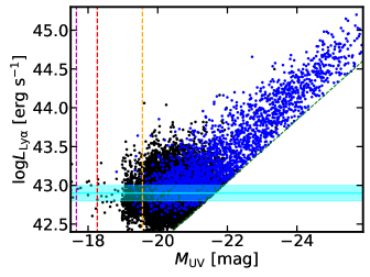
Figure 1: $M_{\mathrm{UV}}-\log L_{\mathrm{Ly\alpha}}$ distributions of our LAE sample. The blue (black) data points denote BL- (NL-) LAEs. The green dashed line indicates our EW${}_{0}>20$ Å cut. The horizontal cyan line corresponds to our $50\%$ $L_{\mathrm{Ly\alpha}}$ detection limit averaged over our redshift range, with cyan shaded regions indicating the $1\sigma$ uncertainty (68.27% equal-tailed credible interval). The magenta, red, and orange vertical dashed lines show the $M_{\mathrm{UV}}$ detection limits in COSMOS, Fall and Spring fields, respectively.

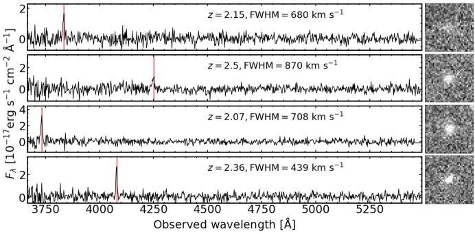
Figure 2: Examples of NL-LAEs. Left panels show the HETDEX spectra (black lines) of NL-LAEs. The redshifts and FWHMs are indicated at the top of each spectrum. The red solid lines represent the wavelengths of Ly$\alpha$ emission lines. Right panels denote the $8^{\prime\prime}\times 8^{\prime\prime}$ $r$-band images from the HETDEX-HSC survey. North is up, and east is to the left.

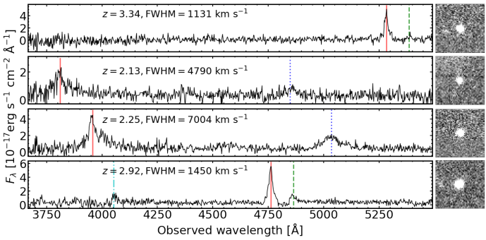
Figure 3: Same as Fig. 2, but for our BL-LAEs. Additionally, the blue dotted lines, green dashed lines, and cyan dash-dotted lines represent the wavelengths of detected Civ, Nv $\lambda 1240$ Å, and Ovi $\lambda 1035$ Å emission lines, respectively.

3.2.3 Summary of Our LAE Sample

Overall, our LAE selection criteria can be summarized as

$$\mathrm{EW_{0}}>20\mathrm{\r{A}}\ \mathrm{and}\\ [(\mathrm{FWHM}\leq 1000\ \mathrm{km\ s^{-1}}\ \mathrm{and}\ P_{\mathrm{{LAE}}}/P_{\mathrm{[OII]}}>1)\\ \mathrm{or}\ (\mathrm{FWHM}>1000\ \mathrm{km\ s^{-1}})]$$ (3)

With this set of criteria, we select $18320$ LAEs from an effective survey area of $11.4$ deg². Our LAE sample includes $16194$ ($2126$) NL- (BL-) LAEs (Table 2). In Figure 1, we show the $M_{\mathrm{UV}}-\log L_{\mathrm{Ly\alpha}}$ distribution of our LAE sample.

It should be noted that our LAEs defined by Eqation 3 represent an EW₀-limited sample of both Ly$\alpha$-emitting SF galaxies and AGN at the bright $L_{\mathrm{Ly\alpha}}$ regime ($L_{\mathrm{Ly\alpha}}\gtrsim 10^{43}$ erg s^-1) that is different from the one of the forthcoming HETDEX studies, which produces a number count offset up to a factor of two.

3.3 Spectroscopic Follow-up of BL-LAE Candidates

To identify the potential Civ emission line of our type 1 AGN candidates, we carried out spectroscopic follow-up observations with the DEpt Imaging Multi Object Spectrograph (DEIMOS) on the Keck 2 Telescope (PI: Y. Harikane). With the criteria mentioned in Section 3.2.2, we select five BL-LAE candidates that are visible during the observations. Our targets are summarized in Table 3.

The observations were conducted on 2020 February 25 (UT) during the filler time of Harikane et al.’s observations when their main targets were not visible. The seeing size is $0^{\prime\prime}.4-0^{\prime\prime}.8$ in FWHM. We used 2 DEIMOS masks, KAKm1 and MUKm1, to cover the 5 objects (Table 3) with the BAL12 filter and the 600ZD grating that is a blue spectroscopy setting for DEIMOS. The slit width was $1^{\prime\prime}.0$. The spatial pixel scale was $0^{\prime\prime}.1181\ \mathrm{pixel}^{-1}$. The spectral range is 4500-8000 Å with a resolution of $R\sim 1500$. We took 5 (4) frames for KAKm1 (MUKm1) with a single exposure time of 2,000 seconds. However, one frame for KAKm1 was affected by the high background sky level. We do not use this frame for our analysis. The total number of frames used for our analyses is 4 for each mask, KAKm1 or MUKm1. The effective exposure time is 8,000 seconds. We acquired data of arc lamps and standard star G191B2B.

Table 3: Targets of our DEIMOS Observations

Object ID	R.A.	Decl.	$z_{\mathrm{Ly\alpha}}$	$F_{\mathrm{Ly\alpha}}$	$r$	$i$	Note
	(J2000)	(J2000)		($10^{-17}$ erg s-1 cm-2)	(mag)	(mag)
ID-1	14:20:11.8258	+52:51:50.4864	2.33	23.04	26.4	26.5	No emission line detected
ID-2	14:19:23.4252	+52:51:50.4864	2.08	344.3	23.5	23.4	No data available
ID-3	14:18:46.2857	+52:41:48.9012	2.27	92.55	23.3	23.2	Foreground galaxy at $z=0.48$
ID-4	14:19:28.9898	+52:49:59.3724	2.31	67.95	22.5	22.5	Type 1 AGN
ID-5	14:18:33.0739	+52:43:13.71	2.14	42.47	23.5	23.1	Type 1 AGN

We obtained spectroscopic data listed in Table 3. Because one out of 5 objects, ID-2, unfortunately fall on the broken CCD of DEIMOS, DEIMOS spectra are available for 4 out of 5 objects. Usually, the DEIMOS spectroscopic data are reduced with the spec2d IDL pipeline (Davis et al., 2003), which performs the bias subtraction, flat fielding, image stacking and wavelength calibration. However, the spec2d pipeline does not work in our blue spectroscopy setting due to the lack of wavelength data in the blue wavelength. We thus carry out the data reduction manually with the IRAF software package (Tody, 1986), using the arc lamps for the wavelength calibration and standard star G91B2B for the flux calibration. We obtain 1D spectra of objects by summing up 15 pixels ($\sim 1^{\prime\prime}.77$) in the spatial direction.

We search for emission lines in both 2D and 1D spectra of the objects listed in 3 at the expected wavelengths, using the redshifts derived from the HETDEX Ly$\alpha$ emission lines. We identify Civ and Ciii] emission lines in two out of the four faint BL-LAE candidates, ID-4 and ID-5. One of the four faint BL-LAE candidates, ID-3, is a foreground galaxy at $z=0.48$ with H$\beta$ and [Oiii] emission lines identified in the DEIMOS spectrum. Another BL-LAE candidate, ID-1, has no detectable emission lines in the DEIMOS spectrum. The $3\sigma$ limiting flux of Civ (Ciii]) of ID-1 is $2.16(1.87)\times 10^{-18}$ erg s^-1 cm^-2. Detailed spectroscopic properties of ID4 and ID5 are presented in Section 5.

4 Deriving the Luminosity Functions

4.1 Contamination

We estimate the contamination rate of our NL- ($f_{\mathrm{NL}}$) and BL-LAEs ($f_{\mathrm{BL}}$) by cross-matching our sample with spectroscopic and/or photometric catalogs. We also explore the morphology of BL-LAEs in archival Hubble Space Telescope (HST) imaging data. Because the number of objects available for $f_{\mathrm{NL}}$ ($f_{\mathrm{BL}}$) estimation is not sufficient to build a redshift and luminosity correlation, we apply a uniform $f_{\mathrm{NL}}$ ($f_{\mathrm{BL}}$) for our NL- (BL-) LAEs. The errors of $f_{\mathrm{NL}}$ and $f_{\mathrm{BL}}$ are based on Poisson statistics.

We estimate $f_{\mathrm{NL}}$ as described in Section 3.2.1. We make a subsample of $32$ NL-LAEs in COSMOS field that are spectroscopically and/or photometrically identified by previous studies. We find that four out of these 32 known galaxies are foreground contaminants. We adopt the $f_{\mathrm{NL}}=13\%\pm 8\%$ ($4/32$) for our NL-LAE subsample.

For BL-LAEs, there are two types of contamination. The first type of contamination is the foreground type 1 AGN whose emission lines are redshifted to the HETDEX spectral range (Section 3.2.2). We estimate the fraction of such contamination $f_{\mathrm{BL,foreground}}$ by crossmatching our BL-LAE subsample with SDSS DR14 QSO catalog (Pâris et al., 2018). Our crossmatching results shows that 111 of our BL-LAEs are previously identified AGN. Among these 111 objects, 99 objects are Ly$\alpha$-emitting AGN at $z=2-3.5$. The remaining 12 objects turn out to be foreground AGN (10 Civ-emitting AGN at $z\sim 1.4$, one Ciii]-emitting AGN at $z\sim 1.0$, and one Mgii-emitting AGN at $z\sim 0.8$). We thus apply $f_{\mathrm{BL,foreground}}=11\%\pm 3\%$ ($12/111$).

The second type of contamination is the broad emission line mimicked by blended narrow lines emitted from close-galaxy pairs on the sky at the similar wavelengths. We examine the morphology of BL-LAE candidates in COSMOS field with archival high-resolution optical images taken with Advanced Camera for Surveys (ACS) on Hubble Space Telescope (Koekemoer et al. 2007; Massey et al. 2010). We find that three out of 10 BL-LAE candidates have multiple components in the HST/ACS images that indicate possible close-galaxy pairs. Because the multiple components do not necessarily all have emission lines, we add errors allowing $f_{\mathrm{close}}$ to range from $0$ to $30\%+20\%$ (3/10). $f_{\mathrm{BL}}$ is obtained by:

$$f_{\mathrm{BL}}=f_{\mathrm{foreground}}+f_{\mathrm{close}}.$$ (4)

4.2 Detection Completeness

For LAEs selected from HETDEX emission line catalog, the detection completeness ($C_{\mathrm{HET}}$) as a function of observed wavelength ($\lambda$) and emission line flux ($F$) is estimated from simulated LAEs inserted into real HETDEX data (Farrow et al., in preparation; Gebhardt et al., in preparation). From $\lambda$ and $F$, we calculate Ly$\alpha$ redshift $z$ and luminosity $L_{\mathrm{Ly\alpha}}$, transforming $C_{\mathrm{HET}}(\lambda,F)$ to $C_{\mathrm{HET}}(z,L_{\mathrm{Ly\alpha}})$. Figure 4 presents an example of $C_{\mathrm{HET}}(z,L_{\mathrm{Ly\alpha}})$.

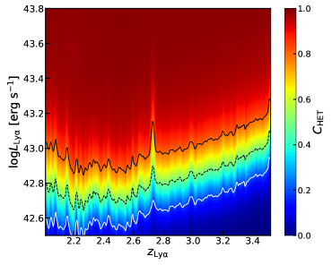
Figure 4: Completeness map of our HETDEX LAEs. The solid white line, dashed black line, and solid black line indicate the $20\%$, $50\%$, and $80\%$ completeness levels, respectively.

For HSC-detected LAEs, the detection completeness $C_{\mathrm{HSC}}$ consists of two completeness values of the HSC $r$-band source detection $C_{\mathrm{HSC,cont}}$ and the HETDEX emission line detection $C_{\mathrm{HSC,line}}$, where

$$C_{\mathrm{HSC}}(z,M_{\mathrm{UV}},L_{\mathrm{Ly\alpha}})=C_{\mathrm{HSC,cont}}(z,M_{\mathrm{UV}})\times C_{\mathrm{HSC,line}}(z,L_{\mathrm{Ly\alpha}}).$$ (5)

We derive $C_{\mathrm{HSC,cont}}$ from Kakuma (2020), who has calculated the completeness of their HSC-SSP $r$-band imaging data as a function of magnitude. We scale their completeness function by the difference of the $5\sigma$ limiting magnitudes between their HSC SSP wide field data ($r_{5\sigma}=25.8$) and our HETDEX-HSC data ($r_{5\sigma}=25.1$), estimating the completeness function of $C_{\mathrm{HSC_{c}ont}}$ that is shown in Figure 5.

We estimate $C_{\mathrm{HSC,line}}$ by Monte Carlo simulations. Specifically, we make $500$ mock spectra with Gaussian line models. For each object in our sample, we fix the FWHM of the line models to the emission line fitting result given in Section 3.1.2. We then produce composite fiber spectra, assuming the 2D light distribution is described by the Moffat PSF with a $2^{\prime\prime}$ FWHM value. We add noise to the composite fiber spectra, randomly generating the noise following a Gaussian distribution function whose sigma is the median value of the noise in the fiber spectra. We perform the emission-line detection on the mock spectra in the same manner as Section 3.1.2, and calculate $C_{\mathrm{HSC,line}}$ that is defined by the fraction of the detected artificial lines to the total mock spectra. We repeat this process with various $z$ and $L_{\mathrm{Ly\alpha}}$, obtaining $C_{\mathrm{HSC,line}}(z,L_{\mathrm{Lya}})$. An example of $C_{\mathrm{HSC,line}}$ is shown in Figure 6.

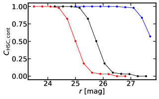
Figure 5: Completeness of our HSC $r$-band imaging data. The blue, black, and red line denote the completeness of imaging data in the COSMOS, Fall, and Spring field, respectively.

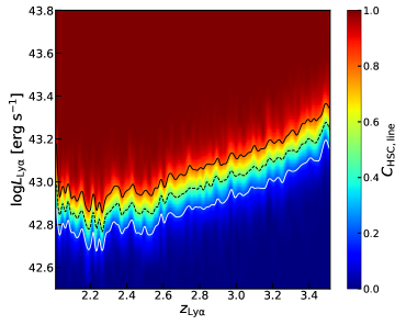
Figure 6: Same as Figure 4, but for our our HSC-detected LAEs.

4.3 Ly$\alpha$ Luminosity Function

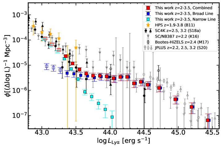
Figure 7: Ly$\alpha$ LF of our NL- (cyan squares), BL- (blue squares) and C-LAEs (red squares) within the $11.4$ deg² survey area. Data points that may affected by incompleteness due to Eddington bias is marked with open squares (see text). For clarity, we slightly shift the data points of NL- and BL-LAEs along the abscissa. The orange stars indicate the results from previous spectroscopic study of Blanc et al. (2011) at $1.9<z<3.8$ (B11). We also show the Ly$\alpha$ LFs at $\log L_{\mathrm{Ly\alpha}}[\mathrm{erg~{}s^{-1}}]\gtrsim 43.3$ derived by previous photometric surveys/studies at three redshift slices of $z$ = 2.2 (downwards triangles), 2.4-2.5 (circles), and 3.2 (upwards triangles) that are taken from Konno et al. (2016) (K16, grey solid symbols), Matthee et al. (2017) (M17, black open symbols), Sobral et al. (2018a) (S18a, black solid symbols), and Spinoso et al. (2020) (S20, grey open symbols).

We derive the Ly$\alpha$ LF with our LAE sample. We apply the non-parametric $1/V_{\mathrm{max}}$ estimator (Schmidt, 1968; Felten, 1976) that accounts for the redshift and luminosity dependent selection function of our LAE sample. For the $i$-th object in our LAE sample, $V_{\mathrm{max},i}$ corresponds to the maximum comoving volume inside which it is detectable. The $V_{\mathrm{max},i}$ value depends on the detection completeness functions $C_{\mathrm{HET}}(z,L_{\mathrm{Ly\alpha}})$ and $C_{\mathrm{HSC}}(z,M_{\mathrm{UV}},L_{\mathrm{Ly\alpha}})$,

$$V_{\mathrm{max},i}=\omega\int_{z_{\mathrm{min}}}^{z_{\mathrm{max}}}C_{i}\frac{\mathrm{d}V}{\mathrm{d}z}\mathrm{d}z,$$ (6)

where $\omega$ and $\frac{dV}{dz}$ denote the angular area of the survey and the differential comoving volume element, respectively. Here, $z_{\mathrm{min}}$ ($z_{\mathrm{max}}$) is the lower (upper) limit of the redshift range of the survey. We calculate $V_{\mathrm{max}}$ of each NL- (BL-) LAE, $V^{\mathrm{NL}}_{\mathrm{max}}$ ($V^{\mathrm{BL}}_{\mathrm{max}}$), and obtain the number densities of NL- and BL-LAEs in each luminosity bin with:

$$\phi_{\mathrm{NL}}(\log L_{\mathrm{Ly\alpha}})=\frac{1-f_{\mathrm{NL}}}{\Delta(\log L_{\mathrm{Ly\alpha}})}\sum_{k}\frac{1}{V^{\mathrm{NL}}_{\mathrm{max},k}},$$ (7)

$$\phi_{\mathrm{BL}}(\log L_{\mathrm{Ly\alpha}})=\frac{1-f_{\mathrm{BL}}}{\Delta(\log L_{\mathrm{Ly\alpha}})}\sum_{k}\frac{1}{V^{\mathrm{BL}}_{\mathrm{max},k}},$$ (8)

where $\Delta(\log L_{\mathrm{Ly\alpha}})$ is the luminosity bin width and $k$ is the number of objects in each luminosity bin. The summations in Eqs. (7) and (8) are performed over the $k$ objects in each luminosity bin.

Figure 7 shows the binned Ly$\alpha$ LF of our LAE sample at $43.0<\log L_{\mathrm{Ly\alpha}}[\mathrm{erg~{}s^{-1}}]<\mathbf{45.5}$, where our LF reaches $50\%$ completeness. Note that at $\log L_{\mathrm{Ly\alpha}}<43.3$ erg s^-1, our Ly$\alpha$ LFs may suffer from a non-negligible Eddington bias (Eddington, 1913) that is generated from uncertainties in HETDEX spectro-photometry (Gebhardt et al., in preparation). We hence do not include the Ly$\alpha$ LF data points at $43.0<\log L_{\mathrm{Ly\alpha}}/[\mathrm{erg~{}s^{-1}}]<43.3$ into our analysis. The error bars of our results are estimated from the quadrature sum of the Poissonian errors, errors in contamination correction, and flux measurement errors. Our LFs span a wide Ly$\alpha$ luminosity range of $43.3<\log L_{\mathrm{Ly\alpha}}/[\mathrm{erg~{}s^{-1}}]<\mathbf{45.5}$, showing a significant bright-end excess at $\log L_{\mathrm{Ly\alpha}}/[\mathrm{erg~{}s^{-1}}]\gtrsim 43.5$ that is dominated by BL-LAEs who are type 1 AGN with FWHM(Ly$\alpha$)$>$1000 km s^-1.

We compare our results in Figure 7 with those from previous studies at the similar redshift and $L_{\mathrm{Ly\alpha}}$ ranges. At $z\sim 2-3$, Blanc et al. (2011) is the only work that presents the spectroscopically-derived Ly$\alpha$ LF at $\log L_{\mathrm{Ly\alpha}}/[\mathrm{erg~{}s^{-1}}]\gtrsim 43$. Due to the limited survey area of 169 arcmin² and the small sample of 80 LAEs, their LF does not show a bright-end hump and has large errors in the two brightest $L_{\mathrm{Ly\alpha}}$ bins at $\log L_{\mathrm{Ly\alpha}}/[\mathrm{erg~{}s^{-1}}]\sim 43.3-43.6$. Over this $L_{\mathrm{Ly\alpha}}$ range, our results are consistent with theirs while having significantly smaller errors. At $\log L_{\mathrm{Ly\alpha}}/[\mathrm{erg~{}s^{-1}}]\sim 43.3-44$, our Ly$\alpha$ LFs are comparable with previous photometric studies (e.g., Konno et al. 2016; Matthee et al. 2017; Sobral et al. 2018a) given the relatively large scatter in their results, which can possibly be attributed to the different small redshift intervals probed by these NB surveys. At the brightest end with $\log L_{\mathrm{Ly\alpha}}/[\mathrm{erg~{}s^{-1}}]\gtrsim 44$ where BL-LAEs dominate, our LF aligns well with Spinoso et al. (2020), supporting their suggestion that the bright LAEs in their sample are QSOs.

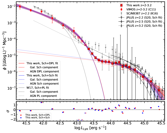
Figure 8: Top: Best-fit Ly$\alpha$ LF of our LAE sample with $2<z<3.2$ (red squares) and Cassata et al. (2011) at $2.0<z<3.2$ (red circles). The red (blue) line shows our best-fit result of Model 1(2) with the measurements of our study and Cassata et al. (2011), with shaded region corresponding to the $1\sigma$ uncertainty (68.27% equal-tailed credible interval). The black open downward triangles (black dashed line), clrcles (solid line), and upward triangles (dotted line) represents the binned Ly$\alpha$ LFs (best Schechter fit) from Spinoso et al. (2020) at $z\sim$ 2.25, 2.54, and 3.24, respectively. The grey triangles indicate the results from Konno et al. (2016). We also show in grey lines the fitting results from Wold et al. (2017) on the obseved Ly$\alpha$ LF of Konno et al. (2016). The dashed, dotted, and solid grey lines indicate their best-fit Schechter component, power law component, and the overall LF, respectively. Bottom: The residuals of Model 1 (red) and 2 (blue) fit in units of the uncertainty in each luminosity bin.

We conduct model fitting with our Ly$\alpha$ LF in Figure 7. In general, Ly$\alpha$ LFs at $\log L_{\mathrm{Ly\alpha}}\lesssim 43.5$ erg s^-1 are well described by the Schechter function. Because our Ly$\alpha$ LF does not cover $\log L_{\mathrm{Ly\alpha}}[\mathrm{erg~{}s^{-1}}]<43.3$, we constrain the faint end of the Ly$\alpha$ LF by including the binned Ly$\alpha$ LF at $z=2-3.2$ from Cassata et al. (2011) in our fitting. The Ly$\alpha$ LF of Cassata et al. (2011) is derived with spectroscopically identified LAEs whose $L_{\mathrm{Ly\alpha}}$ range from 10${}^{41}-10^{43}$ erg s^-1, hence complementary to our sample.

To parameterize the shape of the bright-end hump in our Ly$\alpha$ LF, we considering the following two models separately. In Model 1, we assume the bright-end follows a double power law (DPL) that is broadly used to describe the QSO/AGN UV LF (e.g., Boyle et al. 1988; Pei 1995; Boyle et al. 2000; Richards et al. 2006a; Stevans et al. 2018). The DPL is defined as

$$\phi_{\mathrm{DPL}}(L_{\mathrm{Ly\alpha}})\mathrm{dlog}L_{\mathrm{Ly\alpha}}=\ln 10\ \phi^{*}_{\mathrm{DPL}}\\ \left(\frac{L_{\mathrm{Ly\alpha}}}{L^{*}_{\mathrm{DPL}}}\right)\left[\left(\frac{L_{\mathrm{Ly\alpha}}}{L^{*}_{\mathrm{DPL}}}\right)^{-\alpha_{\mathrm{DPL}}}+\left(\frac{L_{\mathrm{Ly\alpha}}}{L^{*}_{\mathrm{DPL}}}\right)^{-\beta_{\mathrm{DPL}}}\right]^{-1}\mathrm{dlog}L_{\mathrm{Ly\alpha}},$$ (9)

where $L^{*}_{\mathrm{DPL}}$, $\phi^{*}_{\mathrm{DPL}}$, $\alpha_{\mathrm{DPL}}$, and $\beta_{\mathrm{DPL}}$ are characteristic luminosity, the normalization factor, faint-end slope, and bright-end slope, respectively. In Model 2, we assume the bright-end can be described by a Schechter function as suggested by Spinoso et al. (2020).

Table 4: Fitting results of our Ly$\alpha$ LF

Model	Faint Component				Bright Component
	$\alpha$	$\log L^{*}$	$\log\phi^{*}$		$\alpha$	$\beta$	$\log L^{*}$	$\log\phi^{*}$
		[erg s-1]	[Mpc-3]				[erg s-1]	[Mpc-3]
Model 1 (Schechter$+$DPL)	$-1.70_{-0.14}^{+0.13}$	$42.87_{-0.07}^{+0.09}$	$-3.41_{-0.24}^{+0.20}$		$-1.23_{-0.24}^{+0.42}$	$-3.06_{-0.90}^{+0.57}$	$44.68_{-0.40}^{+0.26}$	$-5.92_{-0.32}^{+0.26}$
Model 2 (Schechter$+$Schechter)	$-1.69_{-0.14}^{+0.13}$	$42.86_{-0.07}^{+0.09}$	$-3.39_{-0.23}^{+0.19}$		$-1.27_{-0.19}^{+0.23}$	–	$44.85_{-0.19}^{+0.19}$	$-5.96_{-0.27}^{+0.24}$

We fit our binned Ly$\alpha$ LF with the function of

$$\phi(L_{\mathrm{Ly\alpha}})=\phi_{\mathrm{Faint}}(L_{\mathrm{Ly\alpha}})+\phi_{\mathrm{Bright}}(L_{\mathrm{Ly\alpha}}),$$ (10)

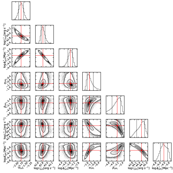
Figure 17: Error contours of our best-fit Ly$\alpha$ LF (Model 1). The red crosses denotes the best-fit results of the parameters. The inner (outer) contour indicates the $68.3\%$ ($95.4\%$) confidence level.

where $\phi_{\mathrm{Faint}}$ represents the Schechter function for the faint component, and $\phi_{\mathrm{Bright}}$ is the DPL (Schechter) function of Model 1(2) for the bright component. We obtain posterior probability distributions for the free parameters in Equation 10 using the Markov Chain Monte Carlo (MCMC) technique. For the prior of $L^{*}_{\mathrm{DPL}}$ and $L^{*}_{\mathrm{Sch}}$ in $\phi_{\mathrm{Bright}}$, we assume uniform distributions that is larger than $L^{*}_{\mathrm{Sch}}$ in $\phi_{\mathrm{Faint}}$ and smaller than the maximum observed $L_{\mathrm{Ly\alpha}}$ ($10^{\mathbf{45.5}}$ erg s^-1) in our Ly$\alpha$ LF. Since the number of our BL-LAEs at the luminosity brighter than the break of DPL in Model 1 is not large, we adopt a uniform prior for $\beta_{\mathrm{DPL}}$ in Model 1 covering a reletively narrow range of $[-5,-2]$ (e.g.,Kulkarni et al. 2019). We assume broad, uniform priors for the other parameters. We use the emcee code (Foreman-Mackey et al., 2013) for MCMC. For each parameter, we adopt the posterior median as our best-fit value and the 68.27% equal-tailed credible interval as the uncertainty. The fitting results of our two models and the best-fit functions are presented in Table 4 and Figures 8, respectively. The posterior probability distributions of the parameters of Model 1(2) are shown in Figure 17 (18). We find that Model 1 can better describe the decay in our Ly$\alpha$ LF at $\log L_{\mathrm{Ly\alpha}}[\mathrm{erg~{}s^{-1}}]\gtrsim 44.8$ with smaller residuals, although the differences are smaller than 1$\sigma$. To compare the performance of the two models, We also calculate the difference in Bayesian information criterion (Schwarz, 1978) that is defined as

$$\Delta\mathrm{BIC}=\chi^{2}_{2}-\chi^{2}_{1}+(k_{2}-k_{1})\ln N.$$ (11)

In Equation 11, $\chi^{2}_{1}$($\chi^{2}_{2}$) and $k_{1}$($k_{2}$) is the $\chi^{2}$ and the number of free parameters of Model 1(2), respectively, and $N$ represents the number of data points that are used in the fitting. We find a $\Delta\mathrm{BIC}$ value of -2.17, suggesting that Model 1 is slightly favored over Model 2. We hence choose Model 1 (Schechter + DPL fit) as the best-fit model of our Ly$\alpha$ LF in the following discussions, although we cannot rule out a Schechter exponential decay of the Ly$\alpha$ LF at $\log L_{\mathrm{Ly\alpha}}[\mathrm{erg~{}s^{-1}}]\gtrsim 45.8$ as described by Model 2.

We compare our best-fit model of Ly$\alpha$ LFs with previous studies. For the bright DPL component, our faint-end slope $\alpha_{\mathrm{DPL}}$ is consistent with the results from Spinoso et al. (2020), who found an weighted-average $\alpha$ value of $-1.35\pm 0.84$ over their four redshift slices. For the faint component, our results have reasonably well constrained Shechter parameters $L^{*}_{\mathrm{Sch}}$, $\alpha_{\mathrm{Sch}}$, and $\phi^{*}_{\mathrm{Sch}}$ that are consistent with Cassata et al. (2011). We note that Cassata et al. (2011) fit their LF with a fixed $L^{*}$ due to the lack of data at the bright end ($L_{\mathrm{Ly\alpha}}>10^{43}$ erg s^-1). Our results provide strong constraints at $L_{\mathrm{Ly\alpha}}>L^{*}_{\mathrm{Sch}}$, determining the best-fit Shechter function by fitting three Schechter parameters simultaneously.

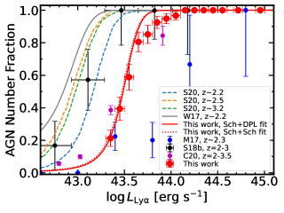
Figure 9: AGN number fraction as a function of $\log L_{\mathrm{Ly\alpha}}$. Our results derived with Equation 12 are shown in the red circles. The functional form of our $f_{\mathrm{AGN,Ly\alpha}}$ derived with Equation 13 using Model 1(2) is presented in the red solid (dashed) line. The other symbols represent previous measurements whose references are listed in the legend. M17: Matthee et al. (2017); W17: Wold et al. (2017); S18: Sobral et al. (2018b); C20: Calhau et al. (2020).

From our binned and best-fit Ly$\alpha$ LFs, we investigate the type 1 AGN number fraction ($f_{\mathrm{AGN,Ly\alpha}}$) of our LAE sample. Note that our $f_{\mathrm{AGN,Ly\alpha}}$ only accounts for type 1 AGN and hence represents the lower limit. First, we calculate $f_{\mathrm{AGN,Ly\alpha}}$ with

$$f_{\mathrm{AGN,Ly\alpha}}(\log L_{\mathrm{Ly\alpha}})=\frac{\phi_{\mathrm{BL}}(\log L_{\mathrm{Ly\alpha}})}{\phi_{\mathrm{BL}}(\log L_{\mathrm{Ly\alpha}})+\phi_{\mathrm{NL}}(\log L_{\mathrm{Ly\alpha}})},$$ (12)

where $\phi_{\mathrm{NL}}$ and $\phi_{\mathrm{BL}}$ are the binned LFs defined in Equation 7 and 8, respectively. We present our results with those estimated with various types of AGN in Figure 9. Our $f_{\mathrm{AGN,Ly\alpha}}$ increases rapidly with $L_{\mathrm{Ly\alpha}}$, rising from $\sim 20\%$ to $\sim 90-100\%$ from $\log L_{\mathrm{Ly\alpha}}/[\mathrm{erg~{}s^{-1}}]\sim 43.3$ to $\sim 43.8$. Such a trend is in good agreement with the results derived with radio and X-ray detected AGN (Calhau et al., 2020). Matthee et al. (2017) also found a similar increase in $f_{\mathrm{AGN,Ly\alpha}}(L_{\mathrm{Ly\alpha}})$ using X-ray detected LAEs. At $\log L_{\mathrm{Ly\alpha}}/[\mathrm{erg~{}s^{-1}}]\sim 43.6-44.4$, their results are lower than ours, which may be attributed to their relatively shallow X-ray and Ly$\alpha$ data (Calhau et al., 2020). Another study that discuss such an increase in $f_{\mathrm{AGN,Ly\alpha}}(L_{\mathrm{Ly\alpha}})$ is Sobral et al. (2018b) based on 21 spectroscopically identified objects that include both type 1 and type 2 AGN. At $\log L_{\mathrm{Ly\alpha}}\leq\ 43.5$ erg s^-1, our $f_{\mathrm{AGN,Ly\alpha}}$ are lower than their results. The small sample and inclusion of type 2 AGN may explain the larger $f_{\mathrm{AGN,Ly\alpha}}$ from Sobral et al. (2018b).

Second, we estimate $f_{\mathrm{AGN,Ly\alpha}}$ with our best-fit Ly$\alpha$ LF, assuming that the faint Schechter component (bright DPL component) can well describe the Ly$\alpha$ LFs of SF galaxies (AGN). The similar method have been applied by Wold et al. (2017) and Spinoso et al. (2020) to derive $f_{\mathrm{AGN,Ly\alpha}}(L_{\mathrm{Ly\alpha}})$. However, as mentioned in Spinoso et al. (2020), $f_{\mathrm{AGN,Ly\alpha}}(L_{\mathrm{Ly\alpha}})$ estimated with this method only represents an illustrative results, given the strong assumption and the high sensitivity to the determination of the faint Schechter component. We calculate $f_{\mathrm{AGN,Ly\alpha}}$ with

$$f_{\mathrm{AGN,Ly\alpha}}(\log L_{\mathrm{Ly\alpha}})=\frac{\phi_{\mathrm{Bright}}(\log L_{\mathrm{Ly\alpha}})}{\phi_{\mathrm{Bright}}(\log L_{\mathrm{Ly\alpha}})+\phi_{\mathrm{Faint}}(\log L_{\mathrm{Ly\alpha}})}.$$ (13)

As shown in Figure 9, our $f_{\mathrm{AGN,Ly\alpha}}(L_{\mathrm{Ly\alpha}})$ estimated with Equation 13 agrees nicely with the ones derived with Equation 12. Comparing with the results from Spinoso et al. (2020) that are based on their bright AGN/QSO LFs and the faint SF galaxy LFs from Sobral et al. (2018a), our $f_{\mathrm{AGN,Ly\alpha}}(L_{\mathrm{Ly\alpha}})$ has a similar increase, and shifts towards brighter $L_{\mathrm{Ly\alpha}}$ by $\Delta\log L_{\mathrm{Ly\alpha}}/[\mathrm{erg~{}s^{-1}}]\sim 0.3-0.5$. Wold et al. (2017) obtained a $f_{\mathrm{AGN,Ly\alpha}}(L_{\mathrm{Ly\alpha}})$ similar to Spinoso et al. (2020), but with a flatter increase, by fitting the observed LF from Konno et al. (2016) that has large scatters at the bright end. They also estimated the observed Ly$\alpha$ luminosity density contributed from SF galaxies ($\rho^{\mathrm{obs}}_{\mathrm{Ly\alpha,SF}}$) and AGN ($\rho^{\mathrm{obs}}_{\mathrm{Ly\alpha,AGN}}$) to be $10^{39.7}$ and $10^{39.5}$ erg s^-1 Mpc^-3, respectively, by integrating their best-fit Ly$\alpha$ LFs over the Ly$\alpha$ luminosity range of $\log L_{\mathrm{Ly\alpha}}=41.41-44.4$ erg s^-1. They concluded that at $z=2.2$, AGN contribute to $\sim 40\%$ to the total observed Ly$\alpha$ luminosity density, which is consistent with their observational results at $z=0.3$ and $z=0.9$. We follow their method, calculating $\rho^{\mathrm{obs}}_{\mathrm{Ly\alpha,SF}}$ and $\rho^{\mathrm{obs}}_{\mathrm{Ly\alpha,AGN}}$ from our best-fit Ly$\alpha$ LF with

$$\rho^{\mathrm{obs}}_{\mathrm{Ly\alpha,SF}}=\int L_{\mathrm{Ly\alpha}}\phi_{\mathrm{Bright}}(L_{\mathrm{Ly\alpha}})\mathrm{d}L_{\mathrm{Ly\alpha}},$$ (14)

$$\rho^{\mathrm{obs}}_{\mathrm{Ly\alpha,AGN}}=\int L_{\mathrm{Ly\alpha}}\phi_{\mathrm{Faint}}(L_{\mathrm{Ly\alpha}})\mathrm{d}L_{\mathrm{Ly\alpha}}.$$ (15)

We integrate Equations (14) and (15) over the same $L_{\mathrm{Ly\alpha}}$ range as mentioned in Wold et al. (2017), obtaining the $\rho^{\mathrm{obs}}_{\mathrm{Ly\alpha,SF}}$ ($\rho^{\mathrm{obs}}_{\mathrm{Ly\alpha,AGN}}$) value of $10^{39.7}$ ($10^{38.6}$) erg s^-1 Mpc^-3. Despite the different shape of best-fit Schechter function as presented in Figure 8, our $\rho^{\mathrm{obs}}_{\mathrm{Ly\alpha,SF}}$ is consistent with the result from Wold et al. (2017). Contrastingly, our $\rho^{\mathrm{obs}}_{\mathrm{Ly\alpha,AGN}}$ is $\sim 10$ times lower, resulting in an AGN contribution of $\sim 8\%$ to the total Ly$\alpha$ luminosity density at $z=2.0-3.2$.

4.4 UV LF

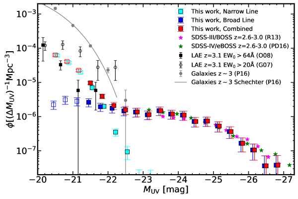
Figure 10: UV LF of our NL- (cyan squares), BL- (blue squares), and C-LAEs (red squares). Data points that may affected by incompleteness is marked with open squares. The magenta and green stars denote the QSO UV LF at $z\sim 2.8$ from SDSS-III (Ross et al. 2013; R13) and SDSS-IV (Palanque-Delabrouille et al. 2016; PD16), respectively. The black squares and black open circles indicate the LAE UV LFs from Ouchi et al. (2008, O08) and Gronwall et al. (2007, G07), respectively. We also show the UV LF of photometrically selected galaxies at $z\sim 3$ in the grey circles and solid line (Parsa et al. 2016; P16).

We derive the UV LF of our LAE sample in the same manner as described in Section 4.3. We convert the $r$-band magnitude ($r$) of our LAEs to the absolute UV magnitude ($M_{\mathrm{UV}}$) using the following relation:

$$M_{\mathrm{UV}}=r-5\log(\frac{d_{\mathrm{L}}}{10\mathrm{pc}})+2.5\log(1+z)+K,$$ (16)

where $d_{\mathrm{L}}$ and $z$ are the luminosity distance in pc and the redshift of our LAEs, respectively, determined by the Ly$\alpha$ emission lines in HETDEX spectra. We set the $K$-correction term ($K$) to be 0 according to our assumption of flat UV continua (Section3.2). Figure 10 presents our UV LF at $-27<M_{\mathrm{UV}}<-21$, where the completeness reaches $50\%$. At the bright end with $M_{\mathrm{UV}}<-22.5$, our results agree well with the SDSS QSO UV LF (Ross et al., 2013; Palanque-Delabrouille et al., 2016). Similar to our Ly$\alpha$ LF, the bright end of our UV LF are dominated by BL-LAEs, indicating the presence of type 1 AGN. At the faint end ($M_{\mathrm{UV}}>-21.5$), our UV LF enters the SF galaxy regime where previous results on the UV LFs of LAEs and photometrically selected are available. Our results are generally consistent with previous UV LFs of LAEs derived by Ouchi et al. (2008) and Gronwall et al. (2007). Our LAE sample may suffer incompleteness at $M_{\mathrm{UV}}>-21.3$ due to the detection limit of Ly$\alpha$ emission lines (Figure 1). As a result, only LAEs with strongest Ly$\alpha$ emission lines are included in our sample. We denote our UV LF at $M_{\mathrm{UV}}>-21.3$ with open symbols.

We study the LAE number fraction ($X_{\mathrm{LAE}}$) as a function of $M_{\mathrm{UV}}$ based on our LAE UV LF ($\phi_{\mathrm{UV,LAE}}$) and the best-fit UV LF of galaxies at $z~{}\sim~{}3$ ($\phi_{\mathrm{UV,z=3}}$) derived by Parsa et al. (2016). They obtained their galaxy sample based on multiband photometry with the photometric redshift determined by SED fitting. By assuming the galaxy sample of Parsa et al. (2016) is complete, we calculate $X_{\mathrm{LAE}}$ with:

$$X_{\mathrm{LAE}}(M_{\mathrm{UV}})=\frac{\phi_{\mathrm{UV,LAE}}(M_{\mathrm{UV}})}{\phi_{\mathrm{UV,z=3}}(M_{\mathrm{UV}})}.$$ (17)

In Figure 11, we present our results covering $-22.1<M_{\mathrm{UV}}<-21.2$, where both our complete LAE UV LF and the galaxy UV LF are available. At $M_{\mathrm{UV}}<-21$, our results show that $X_{\mathrm{LAE}}$ increases towards brighter UV luminosity. Such a trend is mainly due to BL-LAEs, whereas the number fraction of NL-LAEs does not change at $-22.5\lesssim M_{\mathrm{UV}}\lesssim-21$. We compare our results with the $X_{\mathrm{LAE}}$ values derived by two previous studies based on LBG samples at the similar redshift, Stark et al. (2010) and Kusakabe et al. (2020), both of which focused on SF galaxies without AGN. Stark et al. (2010) showed that $X_{\mathrm{LAE}}$ decreases with UV luminosity at $-22.5<M_{\mathrm{UV}}<-18.5$. Their $X_{\mathrm{LAE}}$ at $M_{\mathrm{UV}}=-22$ is in agreement with our results derived from NL-LAEs alone. Contrastingly, Kusakabe et al. (2020) found no UV luminosity dependence of $X_{\mathrm{LAE}}$ at $M_{\mathrm{UV}}\sim-20$ and $-21$, though their values are consistent with those in Stark et al. (2010) within errors. Such a discrepancy may be caused by the increasing LBG selection bias towards faint $M_{\mathrm{UV}}$ (Kusakabe et al., 2020). Our results suggest that while the number fraction of SF-dominated LAEs has a tendency of decrease towards brighter UV luminosity, the number fraction of Ly$\alpha$-emitting type 1 AGN becomes dominant at $M_{\mathrm{UV}}\lesssim-21$ and increases towards brighter UV luminosity. This results in a turnaround of $X_{\mathrm{LAE}}$ at $M_{\mathrm{UV}}\sim-21$.

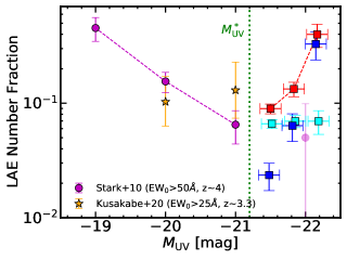
Figure 11: $X_{\mathrm{LAE}}$ as a function of $M_{\mathrm{UV}}$. The red, blue, and cyan squares denote our results derived from C-, BL-, and NL-LAEs, respectively. The magenta circles and yellow stars represent the results from Stark et al. (2010) and Kusakabe et al. (2020), respectively. At $M_{\mathrm{UV}}$ fainter (brighter) than $M^{*}_{\mathrm{UV}}\sim-21$, $X_{\mathrm{LAE}}$ increases (decreases) with $M_{\mathrm{UV}}$.

It should be noted that the UV LF of BL-LAEs shown here is calculated from the total UV flux that includes both AGN and stellar components of host galaxies. In Section 6.2, we evaluate the contributions of UV-continuum emission from AGN and their host galaxies based on SED fitting results from Kakuma (2020), and discuss the redshift evolution of AGN activities.

5 Spectroscopic Properties of BL-LAEs

In this Section, we present spectroscopic properties of the two faint BL-LAEs with spectra, ID-4 and ID-5 (Table 3). We measure the central wavelengths, fluxes, and FWHMs of the Civ and Ciii] emission lines (Figure 12) in the spectra of ID-4 and ID-5 with a best-fit Gaussian profile. We estimate the errors of fluxes and FWHMs by the Monte Carlo simulations. For each emission line, we make 1000 mock emission line spectra by adding noise to the observed line spectrum. The noise added to the observed line spectrum is generated, following a Gaussian probability distribution whose standard deviation is the $1\sigma$ uncertainty in the observed line spectrum. The errors of the measured fluxes and FWHMs are defined as the $68\%$ confidence intervals in the distributions of the fluxes and FWHMs in the mock emission line spectra. We measure the FWHMs of Civ and Ciii], FWHM_CIV and FWHM_CIII], to be $4043.2_{-136.4}^{+138.8}$ $(1072.2_{-104.4}^{+96.8})$ and $4268.0_{-402.4}^{+373.7}$ $(2024.1_{-1202.6}^{+485.6})$ km s^-1, respectively, for ID-4 (ID-5). For the Civ emission line of ID-4, we find a broad component that cannot be well fitted with a single Gaussian profile. We fit the Civ emission line of ID-4 with a double Gaussian profile that consists of a broad and a narrow components, measuring the FWHM with the broad component of the double Gaussian profile. We obtain FWHM_CIV of the broad component is $5536.3_{-185.8}^{+202.1}$ km s^-1. Table 5 summarizes the emission line properties of our objects.

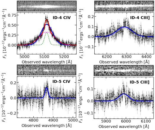
Figure 12: Emission line spectra of ID-4 and ID-5. At the top of each panel, we show the 2D spectrum. At the bottom of each panel, we present the 1D spectrum (black circles with errors) and the best-fit Gaussian profile (blue line). In the top-right panel, we also show the best-fit double Gaussian profile (red line) as well as the broad (cyan dotted line) and the narrow (green dotted line) component.

[t] Object Emission Line Wavelength Flux FWHM Reduced $\chi^{2}$ (Å) ($10^{-17}$ erg s^-1 cm^-2) (km s^-1) ID-4 Civ $5112.9$ $37.83_{-1.00}^{+1.06}$ $4043.2_{-136.4}^{+138.8}$ ($5536.3_{-185.8}^{+202.1}$)^a $1.157$ ($0.861$)^b Ciii] $6287.7$ $9.19_{-0.75}^{+0.77}$ $4268.0_{-402.4}^{+373.7}$ $0.943$ ID-5 Civ $4865.8$ $2.50_{-0.34}^{+0.35}$ $1072.2_{-104.4}^{+95.8}$ $1.043$ Ciii] $5988.6$ $2.50_{-1.00}^{+0.57}$ $2024.1_{-1202.6}^{+485.6}$ $1.326$

Table 5: Emission line properties

• The number in the parenthesis indicate the FWHMs of the broad component in the two-component Gaussian fit.

• The number in the parenthesis indicate the reduced $\chi^{2}$ of the two-component Gaussian fit.

We use the scaling relations of Kim et al. (2018) with $\mathrm{FWHM_{{\sc Civ}}}$ and the monochromatic continuum luminosity at rest-frame 1350Å ($L_{\mathrm{1350}}$) to derive the black hole masses $M_{\mathrm{BH}}$ of ID-4 and ID-5. We estimate $L_{\mathrm{1350}}$ by the log-linear extrapolation from the observed $r$-band and $i$-band fluxes as listed in Table 3. The $M_{\mathrm{BH}}$ value is obtained with:

$$\log\left(\frac{M_{\mathrm{BH}}}{M_{\odot}}\right)=A+\log\left\{\left(\frac{L_{\mathrm{1350}}}{10^{44}\ \mathrm{erg\ s}^{-1}}\right)^{\beta}\left(\frac{\mathrm{FWHM_{CIV}}}{1000\ \mathrm{km\ s}^{-1}}\right)^{\gamma}\right\}.$$ (18)

We adopt the parameters $(A,\beta,\gamma)$ of $(6.7,0.5,2.0)$ that are taken from Kim et al. (2018). Our two faint BL-LAEs, ID-4 and ID-5, have the black hole masses of $\log(M_{\mathrm{BH}}/M_{\odot})=8.70_{-0.03}^{+0.03}$ and $6.85_{-0.08}^{+0.08}$, respectively.

From the $M_{\mathrm{BH}}$ values, we calculate the Eddington ratio ($\lambda_{\mathrm{Edd}}$) of a black hole that is defined as:

$$\lambda_{\mathrm{Edd}}=L_{\mathrm{bol}}/L_{\mathrm{Edd}},$$ (19)

where $L_{\mathrm{bol}}$ ($L_{\mathrm{Edd}}$) is the bolometric (Eddington) luminosity of the black hole. The $L_{\mathrm{bol}}$ are derived from $L_{1350}$ with the bolometric correction factor presented in Richards et al. (2006b) and Shen et al. (2011):

$$L_{\mathrm{bol}}=3.81\times L_{\mathrm{1350}}.$$ (20)

We derive the $L_{\mathrm{bol}}$ values of $10^{45.62}$ ($10^{44.82}$) erg s^-1 for ID-4 (ID-5). The $L_{\mathrm{Edd}}$ is defined as:

$$L_{\mathrm{Edd}}=1.26\times 10^{38}\left(\frac{M_{\mathrm{BH}}}{M_{\odot}}\right).$$ (21)

The Eddington ratios of ID-4 and ID-5 are $\lambda_{\mathrm{Edd}}=0.067_{-0.004}^{+0.005}$ and $=0.746_{-0.121}^{+0.111}$, respectively. Figure 13 presents the $M_{\mathrm{BH}}-L_{\mathrm{bol}}$ relation for ID-4 and ID-5.

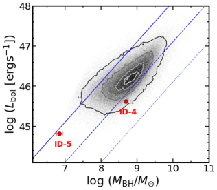
Figure 13: $M_{\mathrm{BH}}-L_{\mathrm{bol}}$ relation for ID-4 and ID-5. The red circles show our measurements. The grey data points and contours represent the results of $z=2-3.5$ quasars in SDSS DR14 (Rakshit et al., 2020). The blue solid, dashed and dotted line correspond to the Eddington ratio $\lambda_{\mathrm{Edd}}=1,0.1$ and $0.01$, respectively.

6 Discussion

6.1 Faint end slope of Ly$\alpha$ LF

Although Gronke et al. (2015) have predicted the evolution of the faint end slope $\alpha_{\mathrm{Sch}}$ of the Ly$\alpha$ LF based on a phenomenological model, such evolution has yet to be confirmed by observations. Combining our Ly$\alpha$ LF at $L_{\mathrm{Ly\alpha}}\geq 10^{43.3}$ erg s^-1 and the one derived by Cassata et al. (2011) at $L_{\mathrm{Ly\alpha}}\leq 10^{43}$ erg s^-1, we reduce the degeneracy in $L^{*}_{\mathrm{Sch}}$ and $\alpha_{\mathrm{Sch}}$ and obtain $\alpha_{\mathrm{Sch}}$ by fitting the three Schechter parameters simultaneously. To study the evolution of the faint end slope of the Ly$\alpha$ LF, we compare our result with $\alpha_{\mathrm{Sch}}$ derived from previous photometric (Konno et al., 2018; Sobral et al., 2018a) and spectroscopic (Drake et al., 2017; Herenz et al., 2019) studies. We fit a linear relationship between $\alpha_{\mathrm{Sch}}$ and $z$ to the measurements from this work and Drake et al. (2017) in Figure 14. Our best-fit linear function has a slope of $-0.38_{-0.26}^{+0.18}$ and an intersection of $-0.71_{-0.60}^{+0.86}$. To evaluate the strength of the linear relation between $\alpha_{\mathrm{Sch}}$ and $z$, we calculate the Pearson correlation coefficient $r$. We obtain the result of $r=-0.72$ with a $p$-value of $0.15$, indicating a marginally significant trend of anti-correlation between $\alpha_{\mathrm{Sch}}$ and $z$. Comparison between the $\alpha_{\mathrm{Sch}}-z$ relation of the Ly$\alpha$ LF and that for the galaxy UV LF (Parsa et al., 2016) suggests that the $\alpha_{\mathrm{Sch}}$ of the Ly$\alpha$ LFs is steeper than that of the galaxy UV LFs. Also, the evolution of $\alpha_{\mathrm{Sch}}$ of the Ly$\alpha$ LF is more rapid than that of galaxy UV LF. The steepening of $\alpha_{\mathrm{Sch}}$ of the Ly$\alpha$ LFs towards higher redshift is consistent with the observational results that dust attenuation of Ly$\alpha$ emission from SF galaxies decreases towards fainter UV luminosity (e.g., Ando et al. 2006; Ouchi et al. 2008) and higher redshift (e.g., Blanc et al. 2011; Hayes et al. 2011). Because SF galaxies become less dusty at higher redshift and lower mass, a larger fraction of faint LAEs are observed towards higher redshift. The increase in the fraction of faint LAEs may contribute to the rapid increase in Ly$\alpha$ escape fraction from $z\sim 2$ to $z\sim 6$ (Konno et al., 2016).

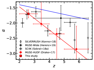
Figure 14: Evolution of the faint end slope of Ly$\alpha$ LF. Our result is denoted by the red square. The red circles, black filled circles, black open circles, and black open diamonds indicate the results from Drake et al. (2017), Herenz et al. (2019), Sobral et al. (2018a), and Konno et al. (2018), respectively. The error bars in the abscissa are the redshift ranges of the measurements. Our best-fit linear function is presented in the red line. The blue solid line shows the redshift evolution of the faint end slope of UV LF derived with photometrically selected galaxies (Parsa et al., 2016).

6.2 Type 1 AGN UV LF and the Evolution

As mentioned in Section 4.4, our UV LFs of BL-LAEs are based on the total flux contributed from both the AGN and stellar components of host galaxies. Here we refer to the type 1 AGN UV LF as the UV LFs of BL-LAE with the flux contributed from the stellar components of galaxies removed. We derive the type 1 AGN UV LFs from UV LFs of BL-LAEs using the AGN UV flux ratio ($f_{\mathrm{flux,AGN}}$) that is defined as the ratio of flux contributed from AGN to the total flux. Specifically, we calculate $f_{\mathrm{flux,AGN}}$ of our BL-LAEs at each $M_{\mathrm{UV}}$ bin based on the results from Kakuma (2020). Kakuma (2020) obtained a sample of 37 type 1 AGN at $z=2-3.5$ using the same method as mentioned in 3.2.2 and conducted SED fitting on their sample with the Code Investigating GALaxy Emission (CIGALE; Boquien et al. 2019). Their results are shown in Figure 15. Assuming a linear relation between $M_{\mathrm{UV}}$ and $\log f_{\mathrm{flux,AGN}}$, we obtain the follwing best-fit model by MCMC:

$$\log f_{\mathrm{UV,AGN}}=-3.056M_{\mathrm{UV}}-0.118$$ (22)

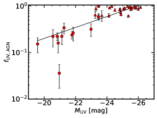
Figure 15: $M_{\mathrm{UV}}-f_{\mathrm{UV,AGN}}$ relation derived by Kakuma (2020). The red circles (triangles) indicate type 1 AGN selected from HETDEX (SDSS). Our best-fit linear function of $\log f_{\mathrm{UV,AGN}}=-3.056M_{\mathrm{UV}}-0.118$ is shown in the black solid line (see text).

We multiply the $M_{\mathrm{UV}}$ of the UV LF in Figure 10 by $f_{\mathrm{flux,AGN}}$, obtaining the type 1 AGN UV LFs as shown in Figure 16. Our results reach the very faint end of UV absolute magnitude at $M_{\mathrm{UV}}\sim\ -20$ and agree well with Bongiorno et al. (2007). Following the procedure mentioned in Section 4.3, we fit our type 1 AGN UV LF with the DPL:

$$\phi_{\mathrm{AGN}}(M_{\mathrm{UV}})\mathrm{d}M_{\mathrm{UV}}=\\ \frac{\phi^{*}_{\mathrm{AGN}}\ \mathrm{d}M_{\mathrm{UV}}}{10^{(\alpha_{\mathrm{AGN}}+1)(M_{\mathrm{UV}}-M^{*}_{\mathrm{AGN}})}+10^{(\beta_{\mathrm{AGN}}+1)(M_{\mathrm{UV}}-M^{*}_{\mathrm{AGN}})}},$$ (23)

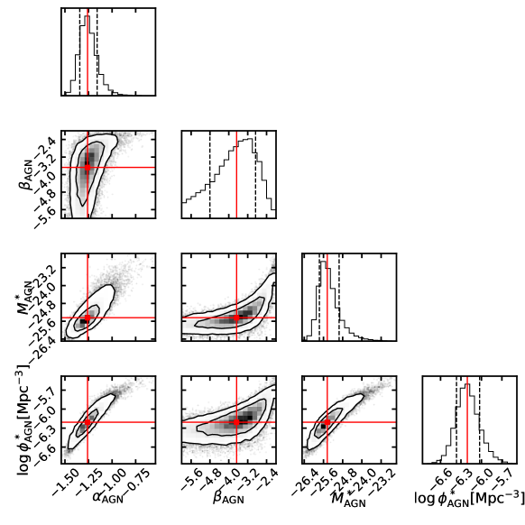
Figure 19: Same as Figure 17, but for type 1 AGN UV LF.

and obtain the best-fit parameters $\alpha_{\mathrm{AGN}}=-1.26^{+0.10}_{-0.08}$, $\beta_{\mathrm{AGN}}=-3.67^{+0.80}_{-1.13}$, $M^{*}_{\mathrm{AGN}}=-25.44^{+0.50}_{-0.33}$, and $\log\phi^{*}_{\mathrm{AGN}}\mathrm{[Mpc^{-3}]}=-6.21^{+0.18}_{-0.16}$. Our best-fit AGN UV LF and the posterior distributions of the parameters are shown in Figure 16 and Figure 19, respectively. We compare our results with Ross et al. (2013) and Palanque-Delabrouille et al. (2016), who studied the QSO UV LF using the pure luminosity evoution (PLE) model and the luminosity evolution and density evolution (LEDE) model. As presented in Figure 16, our type 1 AGN UV LF is consistent with the LEDE model of Ross et al. (2013) at $z=2.75$, suggesting that the AGN UV LF evolve in both luminosities and number densities. We also compare our LFs at $z=2-3$ with those at low redshifts, the type 1 AGN UV LF at $0.1<z<0.4$ (Kulkarni et al., 2019) and type 1 Seyfert UV LF at $0<z<0.15$ (Hao et al., 2005). In Figure 16, a strong evolution of type 1 AGN UV LFs is identified. At the bright end with $M_{\mathrm{UV}}<-22$, we reproduce previous results that show the decrease of number density towards low redshift. At the faint end with $M_{\mathrm{UV}}>-22$, our results show that the number density increases towards low redshift. Such a decrease (increase) of bright (faint) AGN number density towards low redshift can be interpreted as the AGN downsizing effect. First identified in X-ray studies (e.g., Hasinger 2008; Silverman et al. 2008), the AGN downsizing effect was observed in the UV LF only in the bright regime with $M_{\mathrm{UV}}\lesssim-21$ (e.g., Hopkins et al. 2007; Croom et al. 2009; Ikeda et al. 2012). Our results further support the AGN downsizing effect for the very faint AGN with the absolute UV magnitude down to $M_{\mathrm{UV}}\sim-20$.

The AGN downsizing effect may be connected with the quenching of massive galaxies that are observed in the local universe (e.g., Granato et al. 2004; Merloni 2004). Massive BHs, which reside in massive host-galaxies, grow at a high accretion rate and make up the bright end of the AGN UV LFs at $z~{}\sim~{}2-3$. Towards lower redshift, the intense AGN activity in massive galaxies may gradually dispel gas from DM halos, resulting in the halt of star formation in the host galaxies as well as the decrease of BH accretion rate. The AGN become dimmer and populate the faint end of the UV LF. On the other hand, the moderate AGN feedback from less massive BHs would allow the host galaxies to keep their gas, supplying fuel to both star formation and BH accretion (e.g., Babić et al. 2007; Hirschmann et al. 2014).

To further investigate the redshift evolution of Ly$\alpha$ and UV LFs within in $z\sim 2-3$, a larger sample of LAE is needed. These analyses will be presented in our future studies that incorporate forthcoming HETDEX data release.

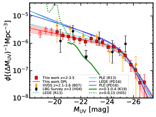
Figure 16: Type 1 AGN UV LF. Our results at $z=2-3.5$ are presented in the red squares. Similar to Figure 10, data points that may be affected by incompleteness are marked with open red squares. The yellow circles denote the AGN UV LF from VVDS survey (Bongiorno et al. 2007; B07) at $z=2.0-3.5$. The black circles indicate the AGN UV LF from LBG survey (Hunt et al. 2004; H04) at $z\sim 3$. The cyan and blue lines are the predicted QSO UV LF at $z=2.75$ from Ross et al. (2013, R13) and Palanque-Delabrouille et al. (2016, PD16), respectively, based on the PLE (solid) and LEDE (dashed) models. The green dashed and solid lines represent the UF LF of type 1 Seyfert galaxies at $0<z<0.15$ (Hao et al. 2005, H05) and the type 1 AGN UV LF at $0.1<z<0.4$ (Kulkarni et al. 2019, K19), respectively.

7 Summary

We investigate the Ly$\alpha$ and UV LFs of LAEs at $z=2-3.5$ that are obtained from the HETDEX spectroscopic survey. Our LAE sample include $16194$ SF galaxies and $2126$ type 1 AGN with EW${}_{0}>20$ Å  that are spectroscopically identified in a sky area of $11.4$ deg². Our main results are summarized below.

We derive the Ly$\alpha$ LF of LAEs at $z=2-3.5$ in the Ly$\alpha$ luminosity range of $43.3<\log L_{\mathrm{Ly\alpha}}[\mathrm{erg\ s^{-1}}]<\mathbf{45.5}$. Our Ly$\alpha$ LF is consistent with those from previous studies. At $\log L_{\mathrm{Ly\alpha}}[\mathrm{erg\ s^{-1}}]>43.5$, our Ly$\alpha$ LF shows a clear bright-end hump. This is the first confirmation of such a bright-end hump with spectroscopically identified LAE samples. We confirm that the bright-end hump can be fully explained by type 1 AGN, which has been suggested in previous studies (e.g., Konno et al. 2016; Matthee et al. 2017; Sobral et al. 2018a; Calhau et al. 2020; Spinoso et al. 2020).

Combining our Ly$\alpha$ LF with the one derived by Cassata et al. (2011), we show that the Ly$\alpha$ LF at $z\sim 2-3$ can be fitted with the combination of the Schechter function and the double power law. Our Ly$\alpha$ LF provides strong constraints at the bright end, reducing the degeneracy of the faint end slope$\alpha_{\mathrm{Sch}}$ and $L^{*}_{\mathrm{Sch}}$ by allowing all three Schechter parameters to be fitted simultaneously. From the Schechter component of our Ly$\alpha$ LF, we measure the faint end slope to be $\alpha_{\mathrm{Sch}}=-1.70^{+0.13}_{-0.14}$ at $z=2-3.2$. We investigate the redshift evolution of $\alpha_{\mathrm{Sch}}$ based on our measurement and those from previous studies. We find that there is a possible redshift evolution of $\alpha_{\mathrm{Sch}}$ over $z\sim 2-6$ with a correlation coefficient $r=-0.72$ at the confidence level of $85\%$. We obtain a linear relation $\alpha_{\mathrm{Sch}}=-0.38_{-0.26}^{+0.18}\ z-0.71_{-0.60}^{+0.86}$ at $z\sim 2-6$. Comparing with the linear relation of $\alpha_{\mathrm{Sch}}$ of the UV LF, we find $\alpha_{\mathrm{Sch}}$ of the Ly$\alpha$ LF may decrease more rapidly towards high redshift.

We derive the UV LF of LAEs at $z=2-3.5$ in the range of $-27<M_{\mathrm{UV}}<20$, connecting the SF galaxy and AGN regimes. Our UV LF are consistent with previous results of QSO UV LF at $M_{\mathrm{UV}}<-23$ and LAE UV LF at $M_{\mathrm{UV}}>-21.5$. Combining our results and the UV LF of galaxies at $z~{}\sim~{}3$, we calculate the LAE number fraction as a function of $M_{\mathrm{UV}}$. Combining with previous measurements, we show that at $M_{\mathrm{UV}}$ fainter (brighter) than $M^{*}_{\mathrm{UV}}\sim-21$, $X_{\mathrm{LAE}}$ decreases (increases) with $M_{\mathrm{UV}}$.

We derive the type 1 AGN UV LF based on the UV LF of LAEs. Our type 1 AGN UV LF reaches a very faint absolute UV magnitude of $M_{\mathrm{UV}}\sim-20$ and agrees well with those from previous studies at similar redshift. Comparing with the results at lower redshifts, we find that the number density of faint ($M_{\mathrm{UV}}>-21$) AGN increases from $z\sim 2$ to $z\sim 0$. Such a number density evolution is compatible with AGN downsizing effect, which may have a close connection with the quenching of galaxy formation.

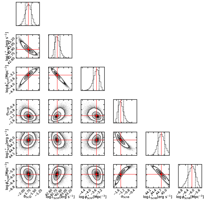
Figure 18: Same as Figure 17, but for Model 2. The Schechter parameters of the faint and bright component are denoted with subscriptions of “SchF” and “SchB”, respectively.

References

- Aihara et al. (2018) Aihara, H., Arimoto, N., Armstrong, R., et al. 2018, PASJ, 70, S4, doi: 10.1093/pasj/psx066
- Aihara et al. (2019) Aihara, H., AlSayyad, Y., Ando, M., et al. 2019, PASJ, 71, 114, doi: 10.1093/pasj/psz103
- Ando et al. (2006) Ando, M., Ohta, K., Iwata, I., et al. 2006, ApJ, 645, L9, doi: 10.1086/505652
- Babić et al. (2007) Babić, A., Miller, L., Jarvis, M. J., et al. 2007, A&A, 474, 755, doi: 10.1051/0004-6361:20078286
- Blanc et al. (2011) Blanc, G. A., Adams, J. J., Gebhardt, K., et al. 2011, ApJ, 736, 31, doi: 10.1088/0004-637X/736/1/31
- Bongiorno et al. (2007) Bongiorno, A., Zamorani, G., Gavignaud, I., et al. 2007, A&A, 472, 443, doi: 10.1051/0004-6361:20077611
- Boquien et al. (2019) Boquien, M., Burgarella, D., Roehlly, Y., et al. 2019, A&A, 622, A103, doi: 10.1051/0004-6361/201834156
- Bosch et al. (2018) Bosch, J., Armstrong, R., Bickerton, S., et al. 2018, PASJ, 70, S5, doi: 10.1093/pasj/psx080
- Bouwens et al. (2015) Bouwens, R. J., Illingworth, G. D., Oesch, P. A., et al. 2015, ApJ, 803, 34, doi: 10.1088/0004-637X/803/1/34
- Boyle et al. (2000) Boyle, B. J., Shanks, T., Croom, S. M., et al. 2000, MNRAS, 317, 1014, doi: 10.1046/j.1365-8711.2000.03730.x
- Boyle et al. (1988) Boyle, B. J., Shanks, T., & Peterson, B. A. 1988, MNRAS, 235, 935, doi: 10.1093/mnras/235.3.935
- Calhau et al. (2020) Calhau, J., Sobral, D., Santos, S., et al. 2020, MNRAS, 493, 3341, doi: 10.1093/mnras/staa476
- Cassata et al. (2011) Cassata, P., Le Fèvre, O., Garilli, B., et al. 2011, A&A, 525, A143, doi: 10.1051/0004-6361/201014410
- Croom et al. (2009) Croom, S. M., Richards, G. T., Shanks, T., et al. 2009, MNRAS, 399, 1755, doi: 10.1111/j.1365-2966.2009.15398.x
- Davis et al. (2003) Davis, M., Faber, S. M., Newman, J., et al. 2003, Society of Photo-Optical Instrumentation Engineers (SPIE) Conference Series, Vol. 4834, Science Objectives and Early Results of the DEEP2 Redshift Survey, ed. P. Guhathakurta, 161–172
- Dawson et al. (2004) Dawson, S., Rhoads, J. E., Malhotra, S., et al. 2004, ApJ, 617, 707, doi: 10.1086/425572
- Deharveng et al. (2008) Deharveng, J.-M., Small, T., Barlow, T. A., et al. 2008, ApJ, 680, 1072, doi: 10.1086/587953
- Dijkstra et al. (2006) Dijkstra, M., Haiman, Z., & Spaans, M. 2006, ApJ, 649, 14, doi: 10.1086/506243
- Drake et al. (2017) Drake, A. B., Garel, T., Wisotzki, L., et al. 2017, A&A, 608, A6, doi: 10.1051/0004-6361/201731431
- Eddington (1913) Eddington, A. S. 1913, MNRAS, 73, 359, doi: 10.1093/mnras/73.5.359
- Fabian (2012) Fabian, A. C. 2012, ARA&A, 50, 455, doi: 10.1146/annurev-astro-081811-125521
- Farrow et al. (2021) Farrow, D. J., Sánchez, A. G., Ciardullo, R., et al. 2021, arXiv e-prints, arXiv:2104.04613. https://arxiv.org/abs/2104.04613
- Felten (1976) Felten, J. E. 1976, ApJ, 207, 700, doi: 10.1086/154538
- Finkelstein et al. (2009) Finkelstein, S. L., Rhoads, J. E., Malhotra, S., & Grogin, N. 2009, ApJ, 691, 465, doi: 10.1088/0004-637X/691/1/465
- Finkelstein et al. (2008) Finkelstein, S. L., Rhoads, J. E., Malhotra, S., Grogin, N., & Wang, J. 2008, ApJ, 678, 655, doi: 10.1086/525272
- Finkelstein et al. (2007) Finkelstein, S. L., Rhoads, J. E., Malhotra, S., Pirzkal, N., & Wang, J. 2007, ApJ, 660, 1023, doi: 10.1086/513462
- Finkelstein et al. (2015) Finkelstein, S. L., Ryan, Russell E., J., Papovich, C., et al. 2015, ApJ, 810, 71, doi: 10.1088/0004-637X/810/1/71
- Foreman-Mackey et al. (2013) Foreman-Mackey, D., Hogg, D. W., Lang, D., & Goodman, J. 2013, PASP, 125, 306, doi: 10.1086/670067
- Gawiser et al. (2006) Gawiser, E., van Dokkum, P. G., Gronwall, C., et al. 2006, ApJ, 642, L13, doi: 10.1086/504467
- Granato et al. (2004) Granato, G. L., De Zotti, G., Silva, L., Bressan, A., & Danese, L. 2004, ApJ, 600, 580, doi: 10.1086/379875
- Gronke et al. (2015) Gronke, M., Dijkstra, M., Trenti, M., & Wyithe, S. 2015, MNRAS, 449, 1284, doi: 10.1093/mnras/stv329
- Gronwall et al. (2007) Gronwall, C., Ciardullo, R., Hickey, T., et al. 2007, ApJ, 667, 79, doi: 10.1086/520324
- Hao et al. (2005) Hao, L., Strauss, M. A., Fan, X., et al. 2005, AJ, 129, 1795, doi: 10.1086/428486
- Harikane et al. (2018) Harikane, Y., Ouchi, M., Shibuya, T., et al. 2018, ApJ, 859, 84, doi: 10.3847/1538-4357/aabd80
- Hasinger (2008) Hasinger, G. 2008, A&A, 490, 905, doi: 10.1051/0004-6361:200809839
- Hayes et al. (2011) Hayes, M., Schaerer, D., Östlin, G., et al. 2011, ApJ, 730, 8, doi: 10.1088/0004-637X/730/1/8
- Herenz et al. (2019) Herenz, E. C., Wisotzki, L., Saust, R., et al. 2019, A&A, 621, A107, doi: 10.1051/0004-6361/201834164
- Hill (2014) Hill, G. J. 2014, Advanced Optical Technologies, 3, 265, doi: 10.1515/aot-2014-0019
- Hill et al. (2008) Hill, G. J., Gebhardt, K., Komatsu, E., et al. 2008, Astronomical Society of the Pacific Conference Series, Vol. 399, The Hobby-Eberly Telescope Dark Energy Experiment (HETDEX): Description and Early Pilot Survey Results, ed. T. Kodama, T. Yamada, & K. Aoki, 115
- Hill et al. (2018a) Hill, G. J., Kelz, A., Lee, H., et al. 2018a, in Society of Photo-Optical Instrumentation Engineers (SPIE) Conference Series, Vol. 10702, Proc. SPIE, 107021K
- Hill et al. (2018b) Hill, G. J., Drory, N., Good, J. M., et al. 2018b, in Society of Photo-Optical Instrumentation Engineers (SPIE) Conference Series, Vol. 10700, Ground-based and Airborne Telescopes VII, ed. H. K. Marshall & J. Spyromilio, 107000P
- Hirschmann et al. (2014) Hirschmann, M., Dolag, K., Saro, A., et al. 2014, MNRAS, 442, 2304, doi: 10.1093/mnras/stu1023
- Hopkins et al. (2007) Hopkins, P. F., Richards, G. T., & Hernquist, L. 2007, ApJ, 654, 731, doi: 10.1086/509629
- Hu et al. (2010) Hu, E. M., Cowie, L. L., Barger, A. J., et al. 2010, ApJ, 725, 394, doi: 10.1088/0004-637X/725/1/394
- Hunt et al. (2004) Hunt, M. P., Steidel, C. C., Adelberger, K. L., & Shapley, A. E. 2004, ApJ, 605, 625, doi: 10.1086/381727
- Ikeda et al. (2012) Ikeda, H., Nagao, T., Matsuoka, K., et al. 2012, ApJ, 756, 160, doi: 10.1088/0004-637X/756/2/160
- Itoh et al. (2018) Itoh, R., Ouchi, M., Zhang, H., et al. 2018, ApJ, 867, 46, doi: 10.3847/1538-4357/aadfe4
- Kakuma (2020) Kakuma, R. 2020, Master’s thesis, The University of Tokyo, Tokyo, Japan
- Kashikawa et al. (2006) Kashikawa, N., Shimasaku, K., Malkan, M. A., et al. 2006, ApJ, 648, 7, doi: 10.1086/504966
- Kashikawa et al. (2012) Kashikawa, N., Nagao, T., Toshikawa, J., et al. 2012, ApJ, 761, 85, doi: 10.1088/0004-637X/761/2/85
- Kelz et al. (2014) Kelz, A., Jahn, T., Haynes, D., et al. 2014, Society of Photo-Optical Instrumentation Engineers (SPIE) Conference Series, Vol. 9147, VIRUS: assembly, testing and performance of 33,000 fibres for HETDEX, 914775
- Kim et al. (2018) Kim, Y., Im, M., Jeon, Y., et al. 2018, ApJ, 855, 138, doi: 10.3847/1538-4357/aaadae
- Koekemoer et al. (2007) Koekemoer, A. M., Aussel, H., Calzetti, D., et al. 2007, ApJS, 172, 196, doi: 10.1086/520086
- Konno et al. (2016) Konno, A., Ouchi, M., Nakajima, K., et al. 2016, ApJ, 823, 20, doi: 10.3847/0004-637X/823/1/20
- Konno et al. (2018) Konno, A., Ouchi, M., Shibuya, T., et al. 2018, PASJ, 70, S16, doi: 10.1093/pasj/psx131
- Kriek et al. (2015) Kriek, M., Shapley, A. E., Reddy, N. A., et al. 2015, ApJS, 218, 15, doi: 10.1088/0067-0049/218/2/15
- Kulkarni et al. (2019) Kulkarni, G., Worseck, G., & Hennawi, J. F. 2019, MNRAS, 488, 1035, doi: 10.1093/mnras/stz1493
- Kusakabe et al. (2020) Kusakabe, H., Blaizot, J., Garel, T., et al. 2020, A&A, 638, A12, doi: 10.1051/0004-6361/201937340
- Laigle et al. (2016) Laigle, C., McCracken, H. J., Ilbert, O., et al. 2016, ApJS, 224, 24, doi: 10.3847/0067-0049/224/2/24
- Leung et al. (2017) Leung, A. S., Acquaviva, V., Gawiser, E., et al. 2017, ApJ, 843, 130, doi: 10.3847/1538-4357/aa71af
- Lusso et al. (2015) Lusso, E., Worseck, G., Hennawi, J. F., et al. 2015, MNRAS, 449, 4204, doi: 10.1093/mnras/stv516
- Malhotra & Rhoads (2004) Malhotra, S., & Rhoads, J. E. 2004, ApJ, 617, L5, doi: 10.1086/427182
- Massey et al. (2010) Massey, R., Stoughton, C., Leauthaud, A., et al. 2010, MNRAS, 401, 371, doi: 10.1111/j.1365-2966.2009.15638.x
- Matthee et al. (2017) Matthee, J., Sobral, D., Best, P., et al. 2017, MNRAS, 471, 629, doi: 10.1093/mnras/stx1569
- Matthee et al. (2018) Matthee, J., Sobral, D., Gronke, M., et al. 2018, A&A, 619, A136, doi: 10.1051/0004-6361/201833528
- Merloni (2004) Merloni, A. 2004, MNRAS, 353, 1035, doi: 10.1111/j.1365-2966.2004.08147.x
- Merloni & Heinz (2013) Merloni, A., & Heinz, S. 2013, Evolution of Active Galactic Nuclei, ed. T. D. Oswalt & W. C. Keel, Vol. 6, 503
- Moffat (1969) Moffat, A. F. J. 1969, A&A, 3, 455
- Nagao et al. (2005) Nagao, T., Motohara, K., Maiolino, R., et al. 2005, ApJ, 631, L5, doi: 10.1086/497135
- Netzer (1990) Netzer, H. 1990, in Act. Galact. Nucl., ed. R. Blandford, H. Netzer, L. Woltjer, T. L. Courvoisier, & M. Mayor, 57–160
- Oke (1974) Oke, J. B. 1974, ApJS, 27, 21, doi: 10.1086/190287
- Ono et al. (2010a) Ono, Y., Ouchi, M., Shimasaku, K., et al. 2010a, ApJ, 724, 1524, doi: 10.1088/0004-637X/724/2/1524
- Ono et al. (2010b) —. 2010b, MNRAS, 402, 1580, doi: 10.1111/j.1365-2966.2009.16034.x
- Ouchi et al. (2020) Ouchi, M., Ono, Y., & Shibuya, T. 2020, ARA&A, 58, 617, doi: 10.1146/annurev-astro-032620-021859
- Ouchi et al. (2008) Ouchi, M., Shimasaku, K., Akiyama, M., et al. 2008, ApJS, 176, 301, doi: 10.1086/527673
- Ouchi et al. (2010) Ouchi, M., Shimasaku, K., Furusawa, H., et al. 2010, ApJ, 723, 869, doi: 10.1088/0004-637X/723/1/869
- Palanque-Delabrouille et al. (2016) Palanque-Delabrouille, N., Magneville, C., Yèche, C., et al. 2016, A&A, 587, A41, doi: 10.1051/0004-6361/201527392
- Pâris et al. (2018) Pâris, I., Petitjean, P., Aubourg, É., et al. 2018, A&A, 613, A51, doi: 10.1051/0004-6361/201732445
- Parsa et al. (2016) Parsa, S., Dunlop, J. S., McLure, R. J., & Mortlock, A. 2016, MNRAS, 456, 3194, doi: 10.1093/mnras/stv2857
- Pei (1995) Pei, Y. C. 1995, ApJ, 438, 623, doi: 10.1086/175105
- Pentericci et al. (2009) Pentericci, L., Grazian, A., Fontana, A., et al. 2009, A&A, 494, 553, doi: 10.1051/0004-6361:200810722
- Rakshit et al. (2020) Rakshit, S., Stalin, C. S., & Kotilainen, J. 2020, ApJS, 249, 17, doi: 10.3847/1538-4365/ab99c5
- Ramsey et al. (1994) Ramsey, L. W., Sebring, T. A., & Sneden, C. A. 1994, Society of Photo-Optical Instrumentation Engineers (SPIE) Conference Series, Vol. 2199, Spectroscopic survey telescope project, ed. L. M. Stepp, 31–40
- Rhoads et al. (2000) Rhoads, J. E., Malhotra, S., Dey, A., et al. 2000, ApJ, 545, L85, doi: 10.1086/317874
- Richards et al. (2006a) Richards, G. T., Strauss, M. A., Fan, X., et al. 2006a, AJ, 131, 2766, doi: 10.1086/503559
- Richards et al. (2006b) Richards, G. T., Lacy, M., Storrie-Lombardi, L. J., et al. 2006b, ApJS, 166, 470, doi: 10.1086/506525
- Ross et al. (2013) Ross, N. P., McGreer, I. D., White, M., et al. 2013, ApJ, 773, 14, doi: 10.1088/0004-637X/773/1/14
- Sakai (2021) Sakai, N. 2021, Master’s thesis, The University of Tokyo, Tokyo, Japan
- Schechter (1976) Schechter, P. 1976, ApJ, 203, 297, doi: 10.1086/154079
- Schmidt (1968) Schmidt, M. 1968, ApJ, 151, 393, doi: 10.1086/149446
- Schwarz (1978) Schwarz, G. 1978, Annals of Statistics, 6, 461
- Shen et al. (2011) Shen, Y., Richards, G. T., Strauss, M. A., et al. 2011, ApJS, 194, 45, doi: 10.1088/0067-0049/194/2/45
- Silverman et al. (2008) Silverman, J. D., Green, P. J., Barkhouse, W. A., et al. 2008, ApJ, 679, 118, doi: 10.1086/529572
- Sobral et al. (2018a) Sobral, D., Santos, S., Matthee, J., et al. 2018a, MNRAS, 476, 4725, doi: 10.1093/mnras/sty378
- Sobral et al. (2017) Sobral, D., Matthee, J., Best, P., et al. 2017, MNRAS, 466, 1242, doi: 10.1093/mnras/stw3090
- Sobral et al. (2018b) Sobral, D., Matthee, J., Darvish, B., et al. 2018b, MNRAS, 477, 2817, doi: 10.1093/mnras/sty782
- Spinoso et al. (2020) Spinoso, D., Orsi, A., López-Sanjuan, C., et al. 2020, arXiv e-prints, arXiv:2006.15084. https://arxiv.org/abs/2006.15084
- Stark et al. (2010) Stark, D. P., Ellis, R. S., Chiu, K., Ouchi, M., & Bunker, A. 2010, MNRAS, 408, 1628, doi: 10.1111/j.1365-2966.2010.17227.x
- Stevans et al. (2018) Stevans, M. L., Finkelstein, S. L., Wold, I., et al. 2018, ApJ, 863, 63, doi: 10.3847/1538-4357/aacbd7
- Tasca et al. (2017) Tasca, L. A. M., Le Fèvre, O., Ribeiro, B., et al. 2017, A&A, 600, A110, doi: 10.1051/0004-6361/201527963
- Tilvi et al. (2020) Tilvi, V., Malhotra, S., Rhoads, J. E., et al. 2020, ApJ, 891, L10, doi: 10.3847/2041-8213/ab75ec
- Tody (1986) Tody, D. 1986, in Society of Photo-Optical Instrumentation Engineers (SPIE) Conference Series, Vol. 627, Instrumentation in astronomy VI, ed. D. L. Crawford, 733
- Trujillo et al. (2001) Trujillo, I., Aguerri, J. A. L., Cepa, J., & Gutiérrez, C. M. 2001, MNRAS, 328, 977, doi: 10.1046/j.1365-8711.2001.04937.x
- Verhamme et al. (2018) Verhamme, A., Garel, T., Ventou, E., et al. 2018, MNRAS, 478, L60, doi: 10.1093/mnrasl/sly058
- Wold et al. (2017) Wold, I. G. B., Finkelstein, S. L., Barger, A. J., Cowie, L. L., & Rosenwasser, B. 2017, ApJ, 848, 108, doi: 10.3847/1538-4357/aa8d6b
- Zheng et al. (2013) Zheng, Z.-Y., Finkelstein, S. L., Finkelstein, K., et al. 2013, MNRAS, 431, 3589, doi: 10.1093/mnras/stt440
- Zheng et al. (2017) Zheng, Z.-Y., Wang, J., Rhoads, J., et al. 2017, ApJ, 842, L22, doi: 10.3847/2041-8213/aa794f