Born in a pair (?): Pisces II and Pegasus III

Abstract

We have used $B,V$ time series photometry collected with the Large Binocular Telescope to undertake the first study of variable stars in the Milky Way ultra-faint dwarf (UFD) satellites, Pisces II and Pegasus III. In Pisces II we have identified a RRab star, one confirmed and a candidate SX Phoenicis star and, a variable with uncertain classification. In Pegasus III we confirmed the variability of two sources: an RRab star and a variable with uncertain classification, similar to the case found in Pisces II. Using the intensity-averaged apparent magnitude of the bona-fide RRab star in each galaxy we estimate distance moduli of $(m-M)_{0}$= 21.22 $\pm$ 0.14 mag (d= 175 $\pm$ 11 kpc) and 21.21 $\pm$ 0.23 mag (d=174 $\pm$ 18 kpc) for Pisces II and Pegasus III, respectively. Tests performed to disentangle the actual nature of variables with an uncertain classification led us to conclude that they most likely are bright, long period and very metal poor RRab members of their respective hosts. This may indicate that Pisces II and Pegasus III contain a dominant old stellar population (t$>$12 Gyr) with metallicity $<[Fe/H]>-$1.8 dex along with, possibly, a minor, more metal-poor component, as supported by the $V$, $B-V$ color-magnitude diagrams of the two UFDs and their spectroscopically confirmed members. The metallicity spread that we derived from our data sample is $\gtrsim$0.4 dex in both systems. Lastly, we built isodensity contour maps which do not reveal any irregular shape, thus making the existence of a physical connection between these UFDs unlikely.

1 Introduction

Extensively under investigation in the last couple of decades, the mechanisms leading to the Milky Way (MW) formation and evolution and the role played by the MW dwarf spheroidal (dSph) satellites in assembling the Galaxy we observe today is still a very hot topic of modern astronomy. Under the current $\Lambda$CDM paradigm, these old satellites could be survivors of the accretion events that led to the formation of the stellar halos of the large galaxies they orbit around (Bullock & Johnston 2005; Sales et al. 2007; Stierwalt et al. 2017). Therefore, the MW dSphs are privileged laboratories, contributing to our understanding of the Universe on both local and cosmological scales. The MW dSphs are close enough to be resolved in stars, thus allowing to study the building up of the MW halo by exploiting information arising from the stars by which they are composed. In the last twenty years, observations carried out by wide-field surveys like the Sloan Digital Sky Survey (SDSS; York et al. 2000) have increased extraordinarily the numbers of companions detected around the MW. Since 2005 the SDSS has revealed that the MW is surrounded by a new class of satellites, the ultra-faint dwarf (UFD) galaxies. UFDs have such low stellar densities to make them very hard to detect unless specific techniques are applied to very large datasets as those provided by the SDSS. This survey in first place, then followed by other imaging surveys such as the Dark Energy Survey (DES; The Dark Energy Survey Collaboration 2005), Pan-STARRS1 3$\pi$ (Chambers et al. 2016), ATLAS (Shanks et al. 2015) and strategic programs like the Subaru Hyper Suprime-Cam Survey (HSC; Aihara, et al. 2018), have increased the number of new MW satellites (UFDs and stellar clusters) up to 47 (Drlica-Wagner et al. 2015; Laevens et al. 2015; Torrealba et al. 2016; Homma, et al. 2019 and references therein). UFDs (see Simon 2019 for a state-of-the-art of the studies on UFDs) are characterised by low surface brightness $\mu_{V}\geq 28$ mag arcsec^-2 and luminosities $-8\leq M_{V}\leq-$1.5 (Martin et al., 2008), hence resulting fainter than all previously known dSphs (hereafter, classical dSphs) and the bulk of Galactic globular clusters (GCs). On the absolute visual magnitude versus half-light radius ($M_{V}$-$r_{h}$) plane, they populate the extension to lower luminosities of the classical dSphs (see, e.g., figure 8 in Belokurov et al. 2007 and figure 3 in Clementini 2010). These systems are believed to be strongly dark matter dominated, as their mass-to-light ratios and velocity dispersions are much higher than for the classical MW satellites (Strigari et al. 2008). Many UFDs present an irregular shape often interpreted as an evidence for tidal interaction with the MW (Belokurov et al., 2007; Muñoz et al., 2010), however their distorted morphologies seem to be more due to lack of deep enough observations rather than the signature of MW tidal stripping (Simon, 2019, and references therein). It has been shown that the metal content in the UFDs is lower than in the classical dSphs and very similar to the chemical composition of extremely metal-poor Galactic halo stars and the most metal-poor Galactic GCs (e.g. Kirby et al. 2008) making them likely the direct descendants of the first generation of galaxies in the Universe (Bovill & Ricotti, 2009; Salvadori & Ferrara, 2009). All UFDs, but Leo T (Clementini et al., 2012), have no signature of ongoing star formation activity and display significant spreads in metallicity spanning [Fe/H] values down to $-$4 dex (see Tolstoy et al. 2009 and references therein). They typically host metal poor ([Fe/H] $\leq-$ 2 dex) populations older than 10 Gyr as revealed by accurate spectroscopic studies of their stellar content (see e.g. Simon & Geha 2007, Kirby et al. 2008, Norris et al. 2010, Simon et al. 2011, Koposov, et al. 2015). Consistently with being populated by an old stellar population and, with the only exceptions of Carina III (Torrealba et al., 2018) and Willman I (Siegel et al., 2008), the UFDs which were studied for variability so far have been found to contain at least one RR Lyrae star. RR Lyrae variables (RRLs) are primary distance indicators and tracers of the oldest stellar population in the systems where they reside. RRLs oscillating in the fundamental (RRab) and first overtone (RRc) pulsation modes occupy two different and well-defined regions in the period-amplitude diagram (Bailey diagram; Bailey 1902; Bailey & Pickering 1913; Bailey et al. 1919). According to the mean period of RRab stars ($\langle P_{ab}\rangle$) and the fraction of RRc stars, the RRLs in the MW field and GCs divide into Oosterhoff type I (Oo I) and Oosterhoff type II (Oo II) groups; this phenomenon is known in the literature as Oosterhoff dichotomy (Oosterhoff, 1939). The Oo I systems are more metal-rich ([Fe/H] $\sim-$1.5 dex), their RRLs have shorter periods ($\langle P_{ab}\rangle\sim$0.55 d) and a fraction of RRc stars around 17$\%$. The Oo II systems are mostly metal-poor ([Fe/H]$\sim-$2.0 dex) with longer RRab periods ($\langle P_{ab}\rangle\sim$0.65 d), bluer horizontal branches (HBs) than the Oo I systems and a higher fraction of RRc stars ($\sim$ 37$\%$). The properties of the RRLs and the Oosterhoff types observed in the MW halo (dSphs, GCs and field) can put constrains on the sub-structures which contributed in the past to the formation of the MW. The photometric studies carried out to define the pulsation properties of the RRLs in the MW satellites have revealed that the classical dSphs do not generally conform to the Oosterhoff dichotomy and, with the exception of Sagittarius and Ursa Minor, are all classified as Oosterhoff-Intermediate (Mateo 1998). Conversely, the UFDs for which a study of the variable stars has been carried out and RRLs have been identified (21 UFDs so far), although containing only very few such variables (hence, a robust Oosterhoff classification is not possible), mainly tend to host RRLs with Oo II properties, as observed for the variables in the MW GCs and halo (Clementini 2010).

In this paper we present a study of the stellar population and variable star content of the Pisces II (Psc II) and Pegasus III (Peg III) UFDs, based on $B,V$ timeseries photometry obtained with the Large Binocular Telescope (LBT). The wide-field of view of the two cameras of the LBT allowed us to image an area corresponding to about 9 half-light radii in each individual pointing of Psc II and of about 12 half-light radii for Peg III. We also investigate the possible physical connection between the two systems from the comparison of their properties (distance, CMDs and variable star populations).

The paper is organised as follows. In Sect. 2 we present an overview of our targets. In Sect. 3 we describe the observations and the data reduction. From Sect. 4 to 7 we discuss results from the identification and characterization of the variable stars, the Oosterhoff classification and measure the distance to Psc II and Peg III using the RRLs. In Sect. 8 we compare the CMDs of Psc II and Peg III with stellar evolution models. In Sec. 9 we discuss the capability to retain and loss metals in low-mass galaxies such as our targets and, in Sect. 10 we present isodensity contour maps. Finally, Sect. 11 summarizes our results.

2 Pisces II and Pegasus III

The Psc II UFD [R.A.(J2000) = 22h58m31s, DEC.(J2000) = 5^∘57^′9^′′; l = 79.21^∘, b = $-$47.11^∘] was discovered in the southern Galactic portion of the SDSS Segue survey (Yanny et al. 2009) by Belokurov et al. (2010), and later studied in more detail by Sand et al. (2012) and Kirby et al. (2015). Using deep wide-field photometry obtained with Megacam at the Magellan Clay telescope, Sand et al. (2012) estimated the structural and photometric parameters of Psc II. From the mean magnitude of the HB they derived the distance modulus of 21.31 $\pm$ 0.17 mag, corresponding to a heliocentric distance of 183 $\pm$ 15 kpc. Sand et al. (2012) also estimated a half-light radius of 1.1 $\pm$ 0.2 arcmin, which delimits the region containing the bulk of the Psc II stars and, at the estimated heliocentric distance, corresponds to a linear extension of 58 $\pm$ 10 pc and an absolute magnitude M_V = $-$4.1 $\pm$ 0.4 mag for Psc II. From the comparison of the galaxy color-magnitude-diagram (CMD) with theoretical isochrones by Girardi et al. (2004) and Dotter et al. (2007, 2008), Sand et al. (2012) concluded that Psc II hosts a dominant old ($>$ 10 Gyr) and metal-poor ([Fe/H]$\sim$ $-$2 dex) stellar population. Kirby et al. (2015) carried out a spectroscopic study of Psc II using the Keck DEIMOS spectrograph. Their radial velocity measurements confirm the membership of seven candidate RGB stars, leading to a systemic velocity $<v_{\bigodot}>$ = $-$226.5 $\pm$ 2.7 kms^-1. They also measured spectroscopic metallicities for four of the seven confirmed members (see Table 1, upper portion), finding an average value of $\langle\rm{[Fe/H]}\rangle$ = $-$2.45 $\pm$ 0.07 dex and a metallicity dispersion of $\sigma$[Fe/H]=0.48$\pm^{0.70}_{0.29}$. Finally, Kirby et al. (2015) estimated the following values for the velocity dispersion $\sigma$ = 5.4${}^{+3.6}_{-2.4}$ kms^-1, dynamical mass log(M_1/2/M_⨀) = 6.2${}^{+0.3}_{-0.2}$ and mass-to light ratio M/L_V = 370${}^{+310}_{240}$ M_⨀/L_⨀, hence confirming that Psc II is a dark matter dominated system.

Table 1: Members of Psc II and Peg III identified by literature spectroscopic studies.

ID	RA (J2000)	DEC (J2000)	$v_{\bigodot}$	[Fe/H]
Pisces II (Kirby et al., 2015)
M1-9004	344.57314	5.92161	$-$224.9$\pm$1.6	$-$2.38$\pm$0.13
M2-9833	344.58857	5.95573	$-$226.9$\pm$3.2	…
M3-10694	344.60458	5.95572	$-$232.0$\pm$1.6	$-$2.70$\pm$0.11
M4-12924	344.64224	5.96213	$-$221.6$\pm$2.9	$-$2.10$\pm$0.18
M5-13387	344.64976	5.95625	$-$215.8$\pm$7.6	…
M6-13560	344.65311	5.96841	$-$232.6$\pm$5.3	$-$2.15$\pm$0.28
M7-14179	344.66411	5.93354	$-$224.8$\pm$9.6	…
Pegasus III (Kim et al., 2016)
M1	336.09960	5.4118042	$-$226.16$\pm$5.04	$-$2.24$\pm$0.15
M2	336.11029	5.4159619	$-$229.45$\pm$5.29	$-$2.55$\pm$0.15
M3	336.11378	5.4077794	$-$218.51$\pm$3.64	$-$2.55$\pm$0.15
M4	336.09539	5.3958641	$-$234.68$\pm$3.84	…
M5	336.10025	5.424227	$-$218.26$\pm$3.56	$-$2.24$\pm$0.15
M6	336.10207	5.3891321	$-$220.57$\pm$4.71	…
M7∗	336.08666	5.39347	$-$193.35$\pm$22.92	…
M8	336.07518	5.4196487	$-$208.45$\pm$6.66	…

A few years later another new MW UFD, Peg III [ R.A.(J2000) = 22h24m48s, DEC.(J2000) = 5^∘24^′18^′′; l = 69.85^∘, b = $-$41.83^∘] was discovered from an analysis of the SDSS Data Release 10 (DR10; Ahn et al. 2014) and then confirmed with deeper Dark Energy Camera (DECam) follow-up observations by Kim et al. (2015). The physical properties derived for Peg III are very similar to those of other previously known MW UFDs, and indeed, Peg III perfectly locates in the UFD region of the $M_{V}$-$r_{h}$ diagram. A further study of this galaxy was carried out by Kim et al. (2016), who using deeper photometry and spectroscopy data from the Magellan/Baade Telescope Inamori-Magellan Areal Camera & Spectrograph (IMACS) provided a better definition of the Peg III structural and photometric parameters. By fitting the HB fiducial line of the Galactic GC M15 ($\langle\rm{[Fe/H]}\rangle$ = $-$2.42 dex; Bernard et al. 2014) to the blue horizontal branch stars, Kim et al. (2016) derived a distance modulus $(m-M)_{0}$ = 21.66 $\pm$ 0.12 mag corresponding to a heliocentric distance d_⨀ = 215 $\pm$ 12 kpc. Using spectroscopic data obtained with the Keck DEIMOS spectrograph, they also measured the radial velocity of a number of candidate members confirming the membership to Peg III of seven of them and obtaining a systemic velocity of $-$222.5 $\pm$ 2.6 kms^-1. A further candidate member has a radial velocity about 30 kms^-1 larger than the systemic velocity inferred from the other seven stars, hence its actual membership to Peg III remains doubtful. The radial velocities of the 8 stars are listed in Table 1(bottom panel). The position of the spectroscopically confirmed member stars and the comparison of the CMD with the Dartmouth isochrones (Dotter et al., 2008) led Kim et al. (2016) to conclude that Peg III has a dominant old (13.5 Gyr) and metal-poor ($\langle{\rm[Fe/H]}\rangle$ = $-$2.5 dex) stellar population, in excellent agreement with most of the MW UFD satellites.

The new values of the half-light radius (r_h = 0.85 $\pm$ 0.22 arcmin, which at the new heliocentric distance corresponds to r_h = 53 $\pm$ 14 pc) and absolute magnitude ( M_V = $-$3.4 $\pm$ 0.4 mag) do not dramatically change the position of Peg III on the M_V-r_h diagram, and keep the galaxy in the UFD region.

Kim et al. (2016) measured the spectroscopic metal abundance of the four brightest stars among the confirmed members, obtaining metallicity estimations from $-$2.24 $\pm$ 0.15 dex to $-$2.55 $\pm$ 0.15 dex. These values are in good agreement with the metallicity inferred from the fit with the old and metal-poor Dartmouth isochrone. The velocity dispersion $\sigma_{v}$ = $-$5.4${}^{+3.0}_{-2.5}$ km s^-1, the dynamical mass M_1/2 = 1.4${}^{+3.0}_{-1.1}$ $\times 10^{6}M_{\bigodot}$ and the mass-to-light ratio M/L_V = 1470${}^{+5660}_{-1240}$ M_⨀/L_⨀ confirm that Peg III is more dark matter dominated than Psc II. In addition, Kim et al. (2016) provide a density contour map that shows the irregular shape of the Peg III structure, mostly in the outermost regions. This could be the sign of an on-going interaction. Finally, Kim et al. (2015, 2016) noticed that Peg III is spatially close to Psc II. They are separated by only 8.5^∘ on the sky and have fairly similar distances. The spatial separation of the two UFDs is $\sim$43$\pm$19 kpc (Kim et al. 2016). If Psc II and Peg III do indeed form a physical pair they could resemble the case of the Leo IV and Leo V, (de Jong et al. 2010) for which an origin related to a single, tidally disrupted progenitor has been proposed. However, they could also resemble the couple Carina II and Carina III (Torrealba et al., 2018), which have a projected separation of only $18^{\prime}$ on sky, hence smaller than Leo IV and Leo V, but are not a pair of bound systems according to Li et al. (2018). The parameters derived in previous studies of Psc II (Kirby et al. 2015, Sand et al. 2012, Belokurov et al. 2010) and Peg III (Kim et al., 2016) are summarized in Table 2.

Table 2: Main parameters of Psc II and Peg III from literature studies.

Parameter	Pisces II	Pegasus III	Ref.a
RA(J2000)	22h58m31s	22h24m24.48s	1,4
DEC(J2000)	5∘57′9′′	5∘24′18′′	1,4
d⨀ (kpc)	183$\pm$15	215$\pm$12	1,3
MV (mag)	$-$4.1$\pm$0.4	$-$3.4$\pm$0.4	1,3
rh (arcmin)	1.1$\pm$0.2	0.85$\pm$0.22	1,3
rh (pc)	58$\pm$10	53$\pm$1.4	1,3
$\epsilon$	$<0.31$	0.38${}^{+0.22}_{-0.38}$	1,3
$\theta$ (deg)	unconstrained	114${}^{+19}_{-17}$	1,3
M1/2 (106M⨀)	6.2${}^{+0.3}_{-0.2}$ c	1.4${}^{+3.0}_{-1.1}$	1,2
M1/2/L${}_{V}^{b}$ (M⨀/L⨀)	370${}^{+310}_{-240}$	1470${}^{+5660}_{-1240}$	1,2
$<v_{\bigodot}>$ (km s-1)	$-$226.5$\pm$2.7	$-$222.9$\pm$2.6	1,2
$\sigma_{v}$ (km s-1)	5.4${}^{+3.6}_{-2.4}$	5.4${}^{+3.0}_{-2.5}$	1,2
$v_{GSR}$ (km s-1)	$-$79.9$\pm$2.7	$-$67.6$\pm$2.6	1,2
$<[Fe/H]>$ (dex)	$-$2.45$\pm$0.07	$-$2.55$\pm$0.15d	1,2
		$-$2.24$\pm$0.15d

3 LBT observations and PSF photometry of Psc II and Peg III

$B$,$V$ time-series photometry of Psc II was collected with the Large Binocular Cameras (LBCs, Giallongo et al., 2008) of the LBT, program (PI: G. Clementini) which targeted also the MW UFD Peg III. Each LBC has a field of view (FoV) of 23${}^{\prime}\times$23^′ and is equipped with four 2048 $\times$ 4608 pixel EEV CCDs resulting in a 6150 $\times$ 6650 pixel equivalent detector, with a pixel scale of 0.224^′′/pixel. The data consist of 26 $B$ and 26 $V$ images for Psc II and of 28 $B$ and 28 $V$ images for Peg III, each with an exposure time of 180s, acquired over six nights from October to December, 2015. This exposure time allowed us to obtain a signal-to-noise ratio (S/N) $\geqslant$ 50 at $B\sim$22.5-23 mag, which roughly corresponds to the minimum in the $B$ and $V$ light curves of RRLs, according to the Psc II and Peg III distance moduli. Most of the observations were obtained with seeing $\leq$ 1.2 arcsec. This is well suited for our purposes. A log of the Psc II and Peg III observations is provided in Table 3. All images were pre-reduced (bias-subtracted, flat-fielded and astrometrized) by the LBT team through an LBC dedicated pipeline, and then, on each of the four CCDs of the two LBCs, separately, we performed point spread function (PSF) photometry with the DAOPHOT-ALLSTAR-ALLFRAME packages (Stetson 1987, 1994). To transform the instrumental magnitudes to the Johnson standard system we used standard stars selected from the SDSS catalog and the transformation equations available at https://www.sdss3.org/dr8/algorithms/sdssUBVRITransform.php#Lupton2005. We used calibration equations of the form: $B-b$= c_B+m${}_{B}\times$($b-v$) and $V-v$=c_V+m${}_{V}\times$($b-v$), where $B$ and $V$ are the standard Johnson magnitudes of the SDSS stars, and $b$ and $v$ are the instrumental magnitudes in our photometric catalogs. The parameters of the calibration were derived by applying a 3$\sigma$ clipping rejection algorithm to fit the data. The final fit to calibrate the Psc II catalog was obtained using a total of 772 stars and provided the following calibration equations: $B-b$=8.229$-$0.1409$\times$($b-v$) and $V-v$=8.139$-$0.0823$\times$($b-v$), with r.m.s values of 0.034 and 0.024 mag in $B$ and $V$, respectively. For Peg III, the sample used for the final fit contains 669 stars and provided the following calibration equations: $B-b$=8.226$-$0.1348$\times$($b-v$) and $V-v$=8.195$-$0.0728$\times$($b-v$), with the r.m.s. values of 0.03 mag for the $B$ and 0.025 mag for the $V$ magnitudes, respectively. These calibration equations, derived independently for Psc II and Peg III, are fully consistent with each other. Our final $B,V$ combined catalogs of sources observed in the LBT fields centered on Psc II and Peg III contain each more than 28,000 objects. The photometric errors for non variable sources in our catalogues typically range from 0.0015 up to 0.01 mag for B $<$ 20.0 mag, from 0.01 up to 0.15 mag for 20.0 $<$ B $<$ 25 mag, then increase steeply for B $>$ 25 mag. In particular, the photometric errors at the HB level are of about 0.06-0.07 mag in $V$ and $B$ for both galaxies.
Unfortunately, an unexpected rotation of the LBT occurred during the observations of Peg III. Therefore some portions of the FoV covered by our observations were deeper than others, causing the detection of fainter sources in those parts of the sky. This produced a more populated CMD but also fictitious overdensities in the density maps, as we further discuss in Sect 10.

Table 3: Log of observations

Dates	Filter	N	Exposure Time	Seeing
			(s)	(arcsec)
Pisces II
October 2, 2015	B	11	180	1.1-1.3
October 2, 2015	V	11	180	0.9-1.4
November 8, 2015	B	2	180	1.3-2.2
November 8, 2015	V	2	180	1.3-2.2
November 9, 2015	B	6	180	0.7
November 9, 2015	V	6	180	0.7
December 1, 2015	B	4	180	1.1-1.3
December 1, 2015	V	4	180	0.9-1.2
December 2, 2015	B	3	180	1
December 2, 2015	V	3	180	1.1-1.4
Pegasus III
October 2, 2015	B	5	180	1.1-1.3
October 2, 2015	V	5	180	0.9-1.4
November 7, 2015	B	5	180	0.8-1
November 7, 2015	V	5	180	0.8-1
November 8, 2015	B	4	180	1.3-2.2
November 8, 2015	V	4	180	1.3-2.2
November 9, 2015	B	5	180	0.7
November 9, 2015	V	5	180	0.7
December 1, 2015	B	5	180	1.1-1.3
December 1, 2015	V	5	180	0.9-1.2
December 2, 2015	B	4	180	1
December 2, 2015	V	4	180	1.1-1.4

4 Variable stars: identification and pulsation properties

To identify variable stars in Psc II and Peg III we first considered stellar sources with a high value of the variability index computed by DAOMASTER (Stetson 1994) both in the $V$ and $B$ passbands. Then we also checked all stars that in the CMDs of our two targets have colors and magnitudes falling within the edges of the classical instability strip (IS). For Psc II this procedure returned a list of $\sim$ 20 candidate variables with more than 22/24 data points on the light curves which were visually inspected with the GRaphical Analyzer of TImes Series package (GRATIS, Clementini et al. 2000). GRATIS uses the Lomb periodogram (Lomb 1976; Scargle 1982) to obtain a first guess of the star periodicity and then the best fit of the folded light curve with a truncated Fourier series to refine the star period. The final adopted periods were those that minimize the r.m.s scatter of the truncated Fourier series best fitting the data. Taking into account the period, the shape of the light curve, the position on the CMD according to the intensity-averaged $B,V$ magnitudes, we confirmed the variability of three candidates and classified in type two of them: 1 RRab and 1 SX Phoenicis (SX Phe) star, whereas the classification of the third confirmed variable remains uncertain because two alternative periods are equally probable for the star. Correspondingly, this variable could either be a metal poor RRab or an anomalous Cepheid (AC).

Figure 1: $B$ (left panels) and $V$ (right panels) light curves of confirmed and candidate variable stars identified in Psc II. For V4 the data have been folded according to the two equally probable periods (bottom two panels). Typical internal errors of the single-epoch data range from 0.01 to 0.07 mag in $B$, and from 0.01 to 0.03 mag in $V$ for the bright variables (V1 and V4) and from 0.03 to 0.30 mag in $B$ and from 0.04 to 0.19 mag in $V$, for the SX Phe stars (V2 and V3).

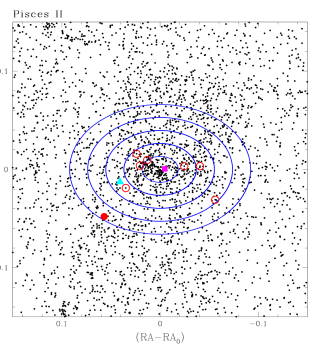
Figure 2: Map of the sources measured in the LBC FoV of Psc II with respect to the galaxy center coordinates. Only sources selected according to the cuts described in Sect. 8 are displayed. Five blue ellipses are drawn showing from one (inner ellipse) to 5 times the galaxy r_h (outer ellipse; that is where V4, the outermost variable of Psc II is located) adopting the position angle, r_h, ellipticity, and center coordinates of Sand et al. (2012). A magenta filled square marks the fundamental mode RRL (V1), a cyan filled triangle the confirmed SX Phe star (V3) and a red filled circle the RRab/AC star (V4). Red open circles show 7 members of Psc II spectroscopically confirmed by Kirby et al. (2015).

Since the available data did not allow us to firmly establish the correct periodicity, hence classification in type, of this source, in this work we used both periodicities to fold the star light curves. A forth source, which is located inside the galaxy r_h, exhibits variability particularly in the $B$ passband. We tentatively classified this source as an SX Phe star, however, this classification remains doubtful because the $V$ light curve shows very little, if any, variability (see Fig. 1). The $B$, $V$ time-series photometry of the variable stars identified in Psc II is provided in the upper portion of Table 4. The properties of the variable stars are summarised in the upper portion of Table 5. Column 1 of Table 5 provides the star identifier. This is an increasing number starting from the galaxy center, for which we have adopted the coordinates of the discovery paper (Belokurov et al. 2010). Columns 2 and 3 give the star coordinates. Columns 4, 5 and 6 list respectively the classification in type, the period (P) and the Heliocentric Julian Day (HJD) of maximum light. Columns 7, 8, 9 and 10 provide the intensity-averaged mean $B$ and $V$ magnitudes and the corresponding amplitudes of the light variation. The $B$, $V$ light curves of the confirmed (3) and candidate (1) variable stars in Psc II are shown in Fig. 1. The spatial distribution of all stars measured in our LBT observations of Psc II with respect to galaxy center (RA₀, DEC₀) is shown in Fig. 2. In the figure we have marked in blue five ellipses representing from one to five times the r_h of Psc II, 1.1 $\pm$ 0.2 arcmin, as estimated by Sand et al. (2012). The bona-fide RRab star (V1; magenta filled square) is located within the Psc II r_h, at a distance from the center of about 0.3^′. The SX Phe star (V3; cyan triangle) and the variable with uncertain type (V4; red filled circle) both are outside the galaxy r_h, at distances of about 2.6^′ and 4.5^′ from the galaxy center. In particular, the SX Phe star is within 3 r_h and the variable with uncertain type within 5 r_h. The distance from the galaxy center and the position on the CMD (see Figure 8) of bona-fide RRab and SX Phe stars suggest that they belong to Psc II; conversely, the membership of V4 remains doubtful (see Section 7). In Peg III the same procedure as applied for Psc II allowed us to confirm the variability of two sources in our list of candidates: an RRab star, according to the period, the shape of the light curve, the position on the CMD and the $B$, $V$ mean magnitudes; and a variable star with uncertain classification. As for V4 in Psc II GRATIS finds two equally possible periodicities for the Peg III variable with an uncertain classification. We used both periodicities to fold the star light curves. According to the two different periods, the corresponding amplitudes of the light variation and the $V$ mean magnitude being about 0.3 mag brighter than the HB level in Peg III, similarly to V4 in Psc II, this variable could either be a very metal poor RRab or an AC. A few additional $B$ and $V$ measurements would be sufficient to improve the light curve sampling and the period definition, thus allowing to definitively classify this variable. The $B$ and $V$ time-series photometry and the properties of the two variable stars we have identified in Peg III are provided in the lower portions of Table 4 and 5, respectively. We have named them V1 and V2 according to their distance from the galaxy center for which we adopted the coordinates by Kim et al. (2016). V1 corresponds to the RRab star and V2 is the variable of uncertain type. Their $B$ and $V$ light curves are shown in Fig. 3, where the data of V2 were folded using the periodicity as RRab in the middle panel and the periodicity as AC in the bottom panel. Figure 4 shows the spatial distribution of all the stars measured in our LBT observations with respect to the center of Peg III. We have marked V1 with a red filled circle, V2 with a red open circle, spectroscopically confirmed members (according to Kim et al. 2016) with blue stars and an ambiguous member with an orange star. In the figure, five green ellipses indicate, in increasing order, 1, 2, 3, 5 and 10 times the half-light radius (r_h) of Peg III, r_h = 0.85 $\pm$ 0.22 arcmin as computed by Kim et al. (2016). The two confirmed variable stars lie outside the galaxy’s r_h, at distances from the galaxy center of 2.5$\arcmin$ for the bona-fide RRab and 5.8$\arcmin$ for the uncertain type variable. The bona-fide RRab is within 4 r_h, and its position on the HB (see right panel of Fig. 8) supports its membership to Peg III. On the contrary, V2 lies within 10 r_h (the star was identified in the data set of CCD1) and is about 0.3 mag above the HB level (see right panel of Fig. 8), thus casting doubts on the actual membership to Peg III of this variable. We discuss V2 more in detail in Section  7.

Figure 3: $B$ (left panels) and $V$ (right panels) light curves of the two pulsating variable stars we have identified in Peg III. As for V4 in Psc II, for V2 the data have been folded according to the two equally probable periods (center and bottom panels). Typical internal errors for the single-epoch data range from 0.01 to 0.08 mag in $B$, and from 0.01 to 0.06 mag in $V$.

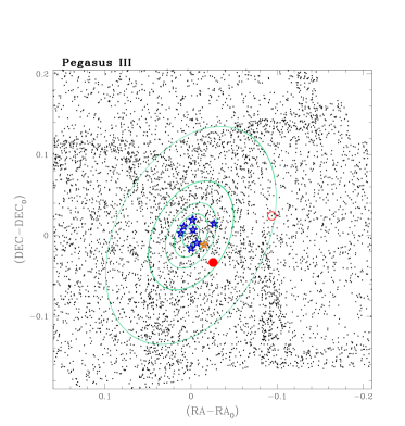
Figure 4: Map of the sources measured in the LBC FoV of Peg III with respect to the galaxy center coordinates. Only sources selected according to the cuts described in Sect. 8 are displayed. We have marked the position of the two confirmed variables using a red filled circle for the RRab star (V1) and a red open circle for V2. We also show the spectroscopically confirmed members (blue stars) and an ambiguous member (orange star) according to Kim et al. (2016). Five green ellipses were drawn convolving the Peg III center coordinates, ellipticity, position angle, r_h, and its multiples, according to the values provided by Kim et al. (2016). The five ellipses correspond to 1, 2, 3, 5 and 10 times the r_h of Peg III.

Table 4: $B$ and $V$ timeseries photometry of the Psc II and Peg III variable stars. The table is published in its entirety in the electronic edition of the journal. A portion is shown here for guidance regarding its form and content.

HJD	B	$\sigma_{B}$	HJD	$V$	$\sigma_{V}$
($-$2457000)	(mag)	(mag)	(-2457000)	(mag)	(mag)
Pisces II - V1
335.60833	21.7788	0.040	335.60828	21.3891	0.0297
335.62004	21.8276	0.036	335.61999	21.4334	0.0275
335.63116	21.9492	0.030	335.63109	21.5478	0.0248
335.63837	22.1282	0.045	335.63831	21.5708	0.0270
335.65506	22.1653	0.065	335.655	21.6142	0.0300
334.58568	22.2208	0.026	334.58562	21.7106	0.0180
334.59818	22.5726	0.039	297.7517	21.7876	0.0213
334.60584	22.5909	0.032	334.59814	21.8667	0.0199
…	…	…	…	…	…

Table 5: Properties of the variable stars identified in Psc II and Peg III

Name	RA	Dec	Type	P	Epoch (max)	$\langle$B$\rangle$	AB	$\langle$V$\rangle$	AV	[Fe/H]∗
	(J2000)	(J2000)		(days)	HJD (2457000)	(mag)	(mag)	(mag)	(mag)	(dex)
Pisces II
V1	22:58:29.858	+5:57:10.92	RRab	0.5551	296.71	22.28	0.94	21.89	0.69	$>-1.6/-1.7$
V2	22:58:33.535	+5:57:43.63	SXPhe(?)	0.04905	…	…	…	…	…
V3	22:58:40.807	+5:56:23.16	SXPhe	0.06348	333.6245	24.245	1.119	23.935	0.775
V4RRL	22:58:44.659	+5:54:16.33	RRab	0.722	335.565	21.98	1.18	21.63	0.93	$>-$2.3
V4AC	22:58:44.659	+5:54:16.33	AC	0.4186	335.612	22.004	1.097	21.635	0.825
Pegasus III
V1	22:24:18.312	+5:22:17.78	RRab	0.5537	357.560	22.58	1.18	22.13	0.96	$>-1.6/-1.7$
V2RRL	22:24:01.932	+5:25:45.52	RRab	0.6594	296.771	22.33	1.26	21.80	1.16	$>-$2.3
V2AC	22:24:01.932	+5:25:45.52	AC	0.3972	357.531	22.37	1.03	21.85	0.84

5 Distance to Psc II and Peg III

We measured the distance to Psc II using V1, the bona-fide RRab star located within the galaxy r_h. The intensity-averaged $V$ magnitude of V1 is $\langle V\rangle$ = 21.890 $\pm$ 0.038 mag (see Table 5), which we de-reddened using a standard extinction law A_V = 3.1 $\times$ E($B-V$) and the reddening value from Schlafly & Finkbeiner (2011), E($B-V$)=0.056 $\pm$0.052 mag. Similar to other nine ultra-faint dwarfs studied by our team (e.g. Dall’Ora et al. 2006; Greco et al. 2008; Clementini et al. 2012; Garofalo et al. 2013 and references therein) we adopted an absolute magnitude M_V = 0.54 $\pm$ 0.09 mag for RRLs with a metallicity of [Fe/H] = $-$1.5 dex (Clementini et al. 2003) and the slope of the luminosity-metallicity relation provided by Clementini et al. (2003) and Gratton et al. (2004), namely $\frac{\Delta M_{V}}{\Delta[Fe/H]}$=0.214 $\pm$ 0.047 mag dex^-1. However, later in the section we consider also more recent calibrations of the absolute magnitude of RRLs which are based on Gaia parallaxes.

A metallicity for V1 to enter the RRL luminosity-metallicity relation, could in principle be obtained from the relation existing between the metal abundance ([Fe/H]), the period and the $\phi_{31}$, parameter of the Fourier decomposition of the $V$-band light curve of RRab stars (Jurcsik & Kovacs 1996). However, this relation cannot be used here because the $V$-band light curve of Psc II V1 (as well as that of Peg III V1) does not satisfy the regularity conditions (Jurcsik & Kovacs 1996; Cacciari et al. 2005) that allow for a reliable application of this method. For the metallicity of Psc II we thus adopt the value [Fe/H]$\sim$ $-$1.7 $\pm$ 0.1 dex which corresponds to the metal abundance of the theoretical isochrones best fitting the galaxy CMD (see Fig. 9, Section 8) dispite the spectroscopic metallicity estimated by Kirby et al. (2015) is much lower ([Fe/H]=$-$2.45$\pm$0.07 dex). The distance modulus we derived for Psc II is then $(m-M)_{0}$= 21.22 $\pm$ 0.14 mag, which corresponds to a distance of d = 175 $\pm$ 11 kpc. If we assume instead the Kirby et al. (2015) spectroscopic metallicity, the distance modulus would be 0.16 mag longer, placing Psc II $\sim$ 14 kpc farther than our previous estimate. Within their respective errors, both these estimates are consistent with Sand et al. (2012)’s distance of 183 $\pm$ 15 kpc which is about in the middle of our estimates.

Gaia second data release in spring 2018 (Gaia DR2, Gaia Collaboration et al., 2018), published trigonometric parallaxes for more than a hundred thousand of sources classified as RRLs. We have adopted the luminosity-metallicity relations from Muraveva et al. (2018), which are calibrated on a sample of 381 Galactic RRLs with Gaia DR2 parallax measurements, to estimate the distance to Psc II (and Peg III). Gaia parallaxes are known to be affected by a global zero-point offset with a mean value $\Delta\varpi_{0}$ = $-$0.03 mas in DR2 (Lindegren et al., 2018; Arenou et al., 2018) and varying as a function of color, magnitude and sky position of the sources. For the RRLs the Gaia DR2 parallax offset ranges from $-0.030$ to $-0.057$ mas (Muraveva et al., 2018). We summarise in Table 6 estimates of the distance modulus for Psc II (upper and middle portions of the table) and Peg III (lower portion), using the bona fide RRL in each galaxy and different choices for the absolute magnitude of RRLs. In particular, the estimates based on Gaia parallaxes are taken from the relations in Muraveva et al. (2018) with parallax offset $\Delta\varpi_{0}=-0.03$, $-0.057$ (value fixed by Muraveva et al. 2018 to infer the linear M${}_{V}-$[Fe/H] relation using a subsample of 23 RRLs with metallicity from high-resolution spectroscopy) and $-0.062$ mas (this is the highest offset value considered by Muraveva et al. 2018 when fitting the linear M${}_{V}-$[Fe/H] relation). Assuming [Fe/H]=$-1.71\pm 0.1$ dex for V1 in Psc II we obtained $(m-M)_{0}$ = 21.12 $\pm$ 0.18 mag for both $\Delta\varpi_{0}=-0.057$ mas and $\Delta\varpi_{0}=-0.062$ mas. These distance moduli place Psc II closer than we find by adopting Clementini et al. (2003) relation, but they are all still compatible within the errors. There is excellent agreement instead between the distance modulus from the Clementini et al. (2003) relation and the value $(m-M)_{0}$ = 21.25 $\pm$ 0.18 mag obtained using the Muraveva et al. (2018) relation with mean offset of $-0.03$ mas (see upper portion of Table 6). Adopting the lower mean metallicity ([Fe/H]=$-2.45\pm 0.07$ dex) spectroscopically determined by Kirby et al. (2015) (middle portion of Table 6), we get identical results using Clementini et al. (2003) relation and Muraveva et al. (2018) relation with parallax offset of $-0.057$ mas. These values are also in good agreement with Sand et al. 2012 estimation. Finally, distance moduli from Muraveva et al. (2018) relations with $\Delta\varpi_{0}=-0.03$ and $\Delta\varpi_{0}=-0.062$ place Psc II, respectively, farther or closer than we find by adopting Clementini et al. (2003) relation, but they are all still compatible within the errors.

Likewise, to estimate the distance to Peg III, we have used the intensity-averaged $V$ magnitude of V1 ($\langle V\rangle$ = 22.126 $\pm$ 0.031 mag, see Table 5), the RRL with a firm classification, which was de-reddened using the reddening value E($B-V$)=0.126$\pm$0.003 mag from Schlafly & Finkbeiner (2011) maps. Then, following the procedure applied for Psc II, we have adopted for the star the metal abundance [Fe/H] = $-$1.6 $\pm$ 0.20 dex, corresponding to the metallicity of the theoretical isochrones best fitting the Peg III CMD (see right panel of Fig. 9). This metallicity is significantly higher than the spectroscopic estimates by Kim et al. (2016) for the kinematically confirmed members of Peg III, which are as low as [Fe/H] = $-$2.55 $\pm$ 0.15 dex, hence, we have used both metallicity values to estimate the distance to Peg III. We find the distance modulus $(m-M)_{0}$ = 21.21 $\pm$ 0.23 mag (d= 174 $\pm$ 18 kpc) adopting for V1 the metal abundance from the isochrone fitting and $(m-M)_{0}$ = 21.42 $\pm$ 0.19 mag (d= 192 $\pm$ 16 kpc) using the spectroscopic metal abundance from Kim et al. (2016). Both values are shorter than the literature value of 215 $\pm$ 12 kpc, however, the latter is consistent with the literature within the errors. Finally, as done for Psc II, we estimated the distance modulus of Peg III from Muraveva et al. (2018) luminosity-metallicity relations and three values ($\Delta\varpi_{0}$ = $-0.03$, $-0.057$ and $-0.062$ mas, respectively) of the Gaia parallax offset (lower portion of Table 6). Again we find that all estimates are consistent within their admittedly large errors, the Gaia parallax zero-point offset $-0.057$ and $-0.062$ mas put Peg III closer than the value obtained from Clementini et al. (2003) relation and, the best agreement is found for $\Delta\varpi_{0}=-0.03$, which leads to: $(m-M)_{0}$ = 21.24 $\pm$ 0.25 mag.

To ease the comparison with our previous studies of RRLs in UFDs, in the following sections we use for the distance moduli of Psc II and Peg III the estimates derived using Clementini et al. (2003) relation.

Table 6: Determinations of the distance modulus for Psc II (upper two portions of the table) and Peg III (lower two portions).

Reference	(m-M)0
	(mag)
Pisces II
assuming [Fe/H] = $-$1.7 $\pm$ 0.1 dex
Clementini et al. (2003)	21.22 $\pm$ 0.14
Muraveva et al. (2018, $\Delta\varpi_{0}=-0.03$)	21.25 $\pm$ 0.19
Muraveva et al. (2018, $\Delta\varpi_{0}=-0.057$)	21.12 $\pm$ 0.18
Muraveva et al. (2018, $\Delta\varpi_{0}=-0.062$)	21.12 $\pm$ 0.18
assuming [Fe/H] = $-$2.45 $\pm$ 0.07 dex
Clementini et al. (2003)	21.38 $\pm$ 0.14
Muraveva et al. (2018, $\Delta\varpi_{0}=-0.03$)	21.53 $\pm$ 0.18
Muraveva et al. (2018, $\Delta\varpi_{0}=-0.057$)	21.31 $\pm$ 0.16
Muraveva et al. (2018, $\Delta\varpi_{0}=-0.062$)	21.38 $\pm$ 0.17
Pegasus III
assuming [Fe/H] = $-$1.6 $\pm$ 0.2 dex
Clementini et al. (2003)	21.21 $\pm$ 0.23
Muraveva et al. (2018, $\Delta\varpi_{0}=-0.03$)	21.24 $\pm$ 0.25
Muraveva et al. (2018, $\Delta\varpi_{0}=-0.057$)	21.11 $\pm$ 0.24
Muraveva et al. (2018, $\Delta\varpi_{0}=-0.062$)	21.11 $\pm$ 0.25
assuming [Fe/H] = $-$2.55 $\pm$ 0.15 dex
Clementini et al. (2003)	21.42 $\pm$ 0.19
Muraveva et al. (2018, $\Delta\varpi_{0}=-0.03$)	21.59 $\pm$ 0.21
Muraveva et al. (2018, $\Delta\varpi_{0}=-0.057$)	21.36 $\pm$ 0.20
Muraveva et al. (2018, $\Delta\varpi_{0}=-0.062$)	21.43 $\pm$ 0.21

6 Bailey diagram and Oosterhoff classification

We have used the $V$-band amplitudes and the periods of the bona-fide RRab stars we have identified in Psc II and Peg III, to plot the stars on the period-amplitude diagram (blue circles and red stars in Fig. 5, respectively) and make a comparison with the RRLs in other MW UFDs.

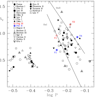
Figure 5: Period-amplitude (Bailey) diagram: the bona fide RRab star inside the r_h of Psc II (star V1) and the variable star with uncertain classification, V4 (plotted adopting the period as RRL, P $=$ 0.722 d) are shown as blue circles, while bona-fide RRab in Peg III, V1, and variable star with uncertain classification, V2 (assuming the period as RRL, P $=$ 0.6594 d) are marked by red stars. Solid lines show the loci of Oo I and Oo II Galactic GCs according to Clement & Rowe (2000). For comparison, we have also plotted the RRLs identified in other 21 MW UFDs (see text for details). We have transformed the SDSS $g$-band amplitudes, A_g, of the RRLs in Gru I, Gru II and Phoenix II, to $V$-band amplitudes, A_V, using a constant ratio, A_g/A_V = 1.2, according to Marconi, et al. (2006, see their Figs. 11 and 12). The Gaia $G$-band amplitudes of the RRLs in Bootes I and III, Coma Berenices, Hydrus I, Tucana II and UMa II reported in Vivas et al. (2020) were converted to A_V amplitudes using eq. 3 in Clementini et al. (2016).

The RRLs detected in other 21 MW UFDs are also plotted in Fig. 5 using different symbols: Coma Berenices (Musella et al., 2009; Vivas et al., 2020), Bootes I (Dall’Ora et al., 2006; Vivas et al., 2020), Bootes II and Bootes III (Sesar et al., 2014; Vivas et al., 2020), Canes Venatici I (Kuehn et al. 2008), Canes Venatici II (Greco et al. 2008), Carina II (Torrealba et al. 2018), Gru I and Gru II (Martínez-Vázquez et al. 2019), Leo IV (Moretti et al. 2009), Leo V (Medina et al., 2017), Hercules (Musella et al., 2012; Garling et al., 2018), Hydra II (Vivas et al. 2016), Hydrus I (Koposov et al., 2018; Vivas et al., 2020), Leo T (Clementini et al. 2012), Phoenix II (Martínez-Vázquez et al. 2019), Segue II (Boettcher et al. 2013), Sagittarius II (Joo et al. 2019), Tucana II (Vivas et al. 2020), Ursa Major I (Garofalo et al. 2013) and Ursa Major II (Dall’Ora et al., 2012; Vivas et al., 2020). In the Bailey diagram fundamental mode and first overtone RRLs lay well separated. As expected for their periods the RRLs we have identified in Psc II and Peg III fall in the region of the fundamental mode pulsators. In Fig. 5 we have highlighted with solid lines the loci of the two Oosterhoff types, Oo I and Oo II, taken from Clement & Rowe (2000). The two bona-fide RRab stars in Psc II and Peg III fall on/close to the Oo I line on the Bailey diagram. This is consistent with the metallicity we have inferred for these two RRLs from the isochrone fitting. Conversely, Psc II-V4 and Peg III-V2 both fall slightly beyond the Oo II locus when adopting for them the periods as RRLs. It is clear from Fig. 5 that UFDs display a large dispersion in the period-amplitude diagram. However, what seems to be unique of Psc II and Peg III is the sharp separation between Oo I and Oo II types of the 2 RRLs each of these UFDs contains (under the assumption that Psc II-V4 and Peg III-V2 are indeed RRLs, see Sect. 7). This seems to differ from what is generally found for other MW UFDs, whose RRLs tend to either lay preferentially between the two Oo lines, like in CVn I (the system which more closely resembles the classical MW dSphs) or to stay closer to just one of them, often the Oo II locus (as in Hercules, Phoenix II, Gru I, Coma Berenices and CVn II).

7 The intriguing cases of V4 in Psc II and V2 in Peg III

As anticipated in Section 4, V4 in Psc II and V2 in Peg III have an uncertain classification. The $B$ and $V$ data of V4 can as well be folded with P $\sim$ 0.72 d and the variable being an RRab star (as well as for V2 in Peg III with P $\sim$ 0.66 d), or with P $\sim$ 0.42 d and the star being a first-overtone AC (as well as for V2 in Peg III with P $\sim$ 0.40 d). ACs have been identified in a number of UFDs (i.e. CVn I, Kuehn et al. 2008; Hercules, Musella et al. 2012; Leo T, Clementini et al. 2012; and Hydra II, Vivas et al. 2016). From an evolutionary point of view ACs can be associated with low metal abundance ([Fe/H]$\leqslant-1.4$ dex) intermediate-age (1-2 Gyr) stellar populations, but neither Psc II nor Peg III show signs of intermediate age population in their CMDs (see Section 8). However, ACs can also be formed by a binary evolution channel. In this case they would not trace a recent star formation episode, but would rather be the product of binary interaction occurred about 1 Gyr ago (Gautschy & Saio, 2017). This formation channel could justify the presence of ACs in systems hosting exclusively old stellar components like GGCs and most of the MW UFDs. We have performed a number of tests to investigate the nature of Psc II-V4 and Peg III-V2. In particular, we have compared them with the $PL$ and $PW$ relations of ACs in the Large Magellanic Cloud (LMC) and, with stellar evolutionary tracks for the typical mass and metallicity of ACs. These comparisons are presented in Appendix. A. They lead us to rule out a classification of V4 and V2 as ACs either belonging to the Psc II and Peg III UFDs or to the field around them.

To explore whether V4 in Psc II and V2 in Peg III can be RRab stars with P=0.722 d and 0.656 d, respectively, we start first from their position on the period-amplitude diagram (Fig. 5). Both stars fall very close to the Oo II locus and have a higher luminosity and lower metallicity than the RRab stars Psc II-V1 and Peg III-V1, which lay instead near the Oo I locus. Variable stars in Oo II clusters have longer periods, higher luminosities and lower metallicities than those in the Oo I clusters (see e.g. Clement & Rowe 2000, and references therein) and are supposed to be evolved off the Zero Age HB (ZAHB; see e.g. Lee et al. 1990). All the properties of V4 and V2 are thus consistent with them being both RRab stars with Oo II characteristics and evolved off the ZAHB. However, as we have already pointed out in Sect. 6, although UFDs do show metallicity spreads as large as 1 dex among their members (see e.g. Simon 2019, and references therein) and large dispersions in the period-amplitude diagrams of their RRLs (Fig. 5), what makes Psc II and Peg III a rather remarkable case is their capability to host RRLs with such distinct Oo properties.

While, it may prove difficult to explain how Psc II and Peg III managed to produce RRLs of both Oosterhoff types (but see Section 9), a further option may be that Psc II-V4 and Peg III-V2 belong to structures/stellar systems projected in front of their hosts. However, there is no sign of an overdensity/structure surrounding V4 in the isodensity contour maps of Psc II (see Fig. 11). Moreover, the distance moduli inferred for Psc II-V1 and V4 appear to be well consistent to each other, within the errors. This is illustrated in Fig. 6, which shows that stellar evolutionary tracks for 0.8 M_⨀ (a typical mass for RRLs) with metallicities corresponding to the metal abundance of V4 (Z=0.00005/[Fe/H]=$-$2.5 dex, violet line; left panel) and V1 (Z=0.0044/[Fe/H]=$-$1.5 dex, orange line; right panel), corrected for the distance modulus of Psc II inferred from V1, well fit the luminosity of both V4 and V1, hence, supporting the conclusion that they are both members of Psc II.

Nevertheless, it remains unclear how the two stars can belong to the same system although they are about 8 kpc apart in projected distance (if we trust the difference in distance moduli, see Section 8) and about 5 r_h apart from the center of Psc II.

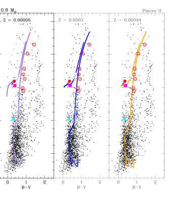
Figure 6: Stellar evolutionary tracks (BaSTI web interface) for 0.8 M_⨀ with Z=0.00005 ([Fe/H]=$-$2.5 dex, violet line; left panel), Z=0.0003 ([Fe/H]=$-$1.8 dex, blue line; central panel) and Z=0.0044 ([Fe/H]=$-$1.5 dex, orange line; right panel). The tracks were corrected adopting the distance modulus of Psc II derived from the RRab star V1 [$(m-M)_{0}$=21.22 mag] and the reddening E$(B-V)$=0.056 mag from Schlafly & Finkbeiner (2011) maps. V1 is marked by a magenta filled square, star V4 by a red filled circle, the SX Phe star (V3) by a cyan filled triangle and the Psc II spectroscopically confirmed members from Kirby et al. (2015) by red open circles.

On the other hand, all variables we have identified in this study are outside the r_h of their hosts (except V1 in Psc II), therefore we cannot rule out they are field stars. Unfortunately, they are fainter than the Gaia limit ($G\leq$ 21 mag; Gaia Collaboration et al., 2018), hence no proper motions are available for them from Gaia to check their membership to Psc II and Peg III. However, we can evaluate the probability they are indeed members of these UFDs by calculating how many field RRLs can be expected in the MW halo at the distance of Psc II and Peg III ($\sim$ 175 kpc). Assuming the radial density distribution of RRLs in the Galactic halo derived by Medina et al. (2018), within 145 kpc from the Galactic center, and considering that these authors have identified 13 RRLs beyond 130 kpc over 120 deg², we found that the number of MW halo RRLs expected at $\sim$ 175 kpc in 0.15 deg² ($\sim$ the LBT FoV) is lower than 10^-9. Therefore, if V4 in Psc II and V2 in Peg III are indeed RRLs, their membership to the corresponding host galaxy is very much plausible.

To conclude, the most likely hypothesis is that Psc II-V4 and Peg III-V2 are RRab stars with Oo II characteristics belonging to respectively the Psc II and Peg III UFDs. However, it remains to clarify how Psc II (and Peg III) can host two stellar populations of different age and metallicity. May two separate star formation episodes have occurred in such small galaxies? This is not quite a common scenario among the MW UFDs (Bland-Hawthorn et al. 2015; Romano et al. 2015 and references therein). We also point out that metallicity is not the only factor that may cause the difference in luminosity among the RRab stars in these galaxies. Other contributors may be evolutionary effects, photometric errors and, in particular, uneven sampling of the light curves. Only the collection of new observations allowing us to definitively pin down the period and classification in type of V4 and V2 may help us clarifying this issue. Adding new data would also help to better constrain the period, amplitude and mean magnitude of the other variable stars we have identified in these UFDs, hence strengthening their classification.

8 Color-Magnitude Diagrams of Psc II and Peg III

The $V$, $B-V$ CMDs of Psc II and Peg III obtained in this study have already been introduced briefly in Sect. 7. We now discuss how they were derived and show them side by side in Figs. 7 and 8 to ease their comparison.

To clean the lists of sources measured in each galaxy we have used the quality information provided by the DAOPHOT quality image parameters $\chi$ and $Sharpness$. Only the stellar detections satisfying the following photometric quality criteria: $-$0.4 $\leq Sharpness\leq$ 0.4, and $\chi<$ 2.2, in both $B$ and $V$ images were retained in the CMDs. This allowed us to reduce the contamination by background galaxies. In Fig. 7 we have plotted all the stellar detections in the LBT FoV for each galaxy, selected according to the above $\chi$ and $Sharpness$ values and separated according to the four CCDs of the LBC mosaic. We note that Milky Way stars dominate the CMDs in Fig. 7 for colors redder than $B-V\sim$1.6 mag. In order to better identify stars belonging to the Psc II galaxy we have cross-matched our catalog against the Kirby et al. (2015) list of spectroscopically confirmed members of Psc II. All the 7 RGB stars which are Psc II members according to Kirby et al. (2015) have a counterpart in our catalog. They are marked by red, empty circles in the left panels of Fig. 7. A magenta square marks V1, the bona-fide RRab star, a red filled circle V4, the variable with less certain classification, both plotted according to their intensity-averaged mean magnitudes computed along the pulsation cycle. A cyan filled triangle shows the SX Phe star (V3). Similarly, in the right panels of Fig 7, the two variables identified in Peg III, V1 and V2, are marked by filled and open red circles, respectively, and plotted according to their intensity-averaged mean magnitudes and colors, the spectroscopically confirmed members by Kim et al. (2016) are marked by blue stars, and an orange star symbol marks the source whose membership is uncertain. Since the ambiguous member lies on the HB region, Kim et al. (2016) speculated that it might be an RRL. Based on our checks of the variability indices in $B$ and $V$ and the visual inspection of the light curves we rule out that this star varies.

Our CMDs of Psc II and Peg III are rather deep, reaching $V\sim$ 26.5 mag, hence they allow us to trace for each galaxy the main sequence (MS) below the turn-off (TO) point, which is located approximately between 25 and 25.5 mag in $V$, according to the theoretical isochrones overlaid on the CMDs (see Fig. 9, later in this section).

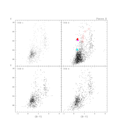
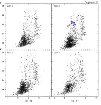
Figure 7: $V$, $B-V$ CMDs of Psc II (on the left) and Peg III (on the right) obtained from data corresponding to the four CCDs of the LBC mosaic, separately. Symbols and color-coding are the same as in Fig. 2 for Psc II and Fig. 4 for Peg III.

As shown by the left panels of Fig. 7, the Psc II galaxy is entirely contained in CCD2, the central CCD of the LBC configuration, where are located all the spectroscopically confirmed members and the variable stars we have identified in Psc II. Only in CCD2 is a hint of the galaxy HB and RGB recognisable (for the latter, the eye is guided by the spectroscopic members). The CMD of Psc II within the half-light radius is very poorly populated; only V1 and one of the 7 spectroscopic members are within the galaxy $r_{h}$, the other six confirmed members are located in the region between 1 and 4 times the galaxy r_h. We have tried to build a final CMD reasonably well populated, which contains all spectroscopic members and the variable stars in the field of Psc II. This is presented in the left panel of Fig. 8, which shows all stellar sources located within 5 times the r_h of the galaxy (all the CMDs shown in the remaining of this section correspond to sources within 5 r_h).

The Peg III UFD is also very small in size (r${}_{h}=53\pm$ 1.4 pc; Kim et al. 2016). As shown by Fig 4 the bona-fide RRab star (V1) and the variable of uncertain classification are located respectively within 5 and 10 times the galaxy r_h, whereas the spectroscopic members are all within 3r_h. Since both spectroscopic members and variable stars are rather far away from the center of Peg III, even more than for Psc II, the CMD we show in the right panel of Fig. 8 contains all stars within 10 times the r_h of Peg III. Furthemore, unlike Psc II, Peg III seems to be not entirely contained in CCD2, as one would expect given its small size. V1 along with the center coordinates of Peg III are within CCD2, whereas V2 is within CCD1. The most recognisable features in the CMDs of Psc II and Peg III are: (i) the HB at $V\sim$ 22 mag (as also inferred from the mean $V$ magnitude of the bona-fide RRab star in each UFD) populated by a few stars close to the red and blue edges of the RRL instability strip and roughly ending at $B-V\sim$ 0.2 mag; (ii) the RGB between ($B-V$)$\sim$0.7 and $\sim$1.4 mag, reaching as bright as $V\sim$ 19.5$-$19 mag, which is disentangled thanks to the RGB member stars by Kirby et al. (2015) for Psc II and Kim et al. (2016) for Peg III. Additionally, in the CMD of Peg III a possible hint of asymptotic giant branch (AGB) or red horizontal branch (RHB) population can be recognised, as also suggested by Kim et al. (2016), thanks to three kinematic members brighter than the HB and bluer than the RGB (colors 0.6 $<$ ($B-V$ ) $<$ 0.8 mag).

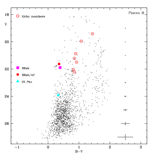
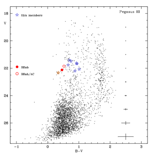
Figure 8: $V$, $B-V$ CMDs showing stellar sources within five times the r_h of Psc II (left panel) and ten times the r_h of Peg III (right panel). Symbols and color-coding are the same as in Figs. 2 and 4.

These features are indicative of a stellar population older than 10 Gyr in both Psc II and Peg III, in agreement with the typical ages of the stellar components observed in other MW UFDs. In order to estimate the age and metallicity of the Psc II and Peg III dominant stellar populations, we have over-plotted on the CMDs the PARSEC stellar isochrones from Bressan et al. (2012), available on the CMD 2.9 web interface. The left panel of Fig. 9 shows the CMD of Psc II in a region within 5 times the galaxy r_h with overlaid the PARSEC isochrones for a fixed age of 13 Gyr (the best-fit we have obtained) and 5 different values of metallicity: [Fe/H] = $-$2.3, $-$1.9, $-$1.8, $-$1.7 and $-$1.5 dex. The isochrones were adjusted to the distance modulus of Psc II (21.22 mag, as inferred from V1, the bona fide RRab star within the galaxy r_h) and a reddening value of E($B-V$)= 0.056 mag from the Schlafly & Finkbeiner (2011) maps. The comparison with the stellar isochrones shows that Psc II hosts a dominant ancient stellar population ($\sim$ 13 Gyr) more metal-rich than [Fe/H]$\sim-$1.8$\pm$0.1 dex, assuming that the bona fide RRab star (magenta square) traces the HB of Psc II and the spectroscopically confirmed members (red empty circles) of Kirby et al. (2015) trace the galaxy RGB. In the right panel of Fig. 9 we show the CMD of Peg III within 10 $r_{h}$, with overlaid PARSEC isochrones for a fixed age of 13 Gyr and metallicities ranging from [Fe/H] = $-$2.2 to $-$1.6 dex. The isochrones were corrected for a reddening E($B-V$)= 0.13 mag from the Schlafly & Finkbeiner (2011) maps and a distance modulus of 21.21 $\pm$ 0.32 mag, as inferred from the bona-fide RRab star in Peg III (V1). The isochrones which better reproduce the RGB and the HB level along with the position of Peg III-V1 are those for metallicities between $-$1.7 and $-$1.6 dex, however the isochrone with [Fe/H] = $-$1.6 dex does not reproduce the overall extension of the HB, which, instead, is well covered by the [Fe/H] = $-$1.7 dex isochrone. The metallicity we find from the isochrone fitting is much higher than the value inferred by Kim et al. (2016) applying the same technique. Using isochrones from Dotter et al. (2008), Kim et al. (2016) suggest as best-fit isochrone for Peg III the one with an age of 13.5 Gyr and metallicity [Fe/H] = $-$2.5 dex. However, we think that the isochrone set with higher metallicity ([Fe/H] = $-$1.5 dex, right panel of fig. 2 in Kim et al. 2016), better reproduces also the CMD by Kim et al. (2016).

In summary, our results from the CMD isochrone fitting suggest that both Peg III and Psc II host a stellar population more metal-rich than derived from spectroscopically confirmed members or by isochrone fitting in previous works. Among the MW UFDs, only Leo T (Clementini et al., 2012) and Ursa Major II (Dall’Ora et al., 2012) have a similarly high metallicity. On the other hand, the comparison with isochrones of different metallicity presented here, the very low metallicity measured for the spectroscopically confirmed members and the position on the period-amplitude diagram also suggest a plausible scenario where V4 in Psc II and V2 in Peg III are very metal-poor ([Fe/H]$>-$2.4 dex) RRab members and tracers of a very metal poor component of these UFDs.

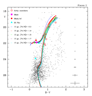
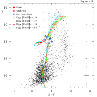
Figure 9: Left: Same as in the left panel of Fig. 8, but with dotted lines showing the PARSEC stellar isochrones (Bressan et al. 2012) for an age of 13 Gyr and metallicities of: [Fe/H] = $-$2.3 dex, blue; [Fe/H] = $-$1.9 dex, orange; [Fe/H] = $-$1.8 dex, green; [Fe/H] = $-$1.7 dex, purple; and [Fe/H] = $-$1.5 dex, cyan. The isochrones were corrected for a distance modulus of 21.22 mag, as derived from the bona fide RRab star (V1) in Psc II, and for a foreground reddening of E($B-V$) = 0.056 mag, according to the Schlafly & Finkbeiner (2011) maps. Right: Same as in the right panel of Fig. 8, dotted lines in different colors are the PARSEC stellar isochrones for an age of 13 Gyr and metallicities of [Fe/H]= $-$1.6, $-$1.7, $-$1.9 and $-$2.2 dex; they were corrected for a distance modulus of 21.21 mag, as inferred from the bona fide RRab star (V1) in Peg III and for a foreground reddening of E($B-V$) = 0.13 mag (Schlafly & Finkbeiner 2011). Symbols and color-coding are the same as in Figs. 2 and 4.

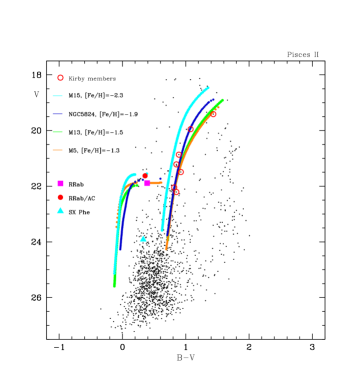
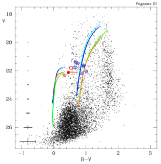
Figure 10: Same as in Fig. 8 but with solid lines showing the ridge lines of the Galactic GCs: M15 (cyan), NGC 5824 (blue), M13 (green), and M5 (orange).

Indeed, as we have shown in Sect. 5, if we adopt for V4 in Psc II the metallicity derived by Kirby et al. (2015, Fe/H=$-$2.45$\pm$0.07 dex) the inferred distance modulus is $(m-M)_{0}$= 21.12 $\pm$ 0.20 mag, which would be consistent, within the errors, with the distance modulus inferred from the more metal rich RRab star V1 (21.22 $\pm$ 0.14 mag). In the same vein, if V2 is a very metal poor ([Fe/H] = $-$2.54 $\pm$ 0.79 dex) RRab star belonging to Peg III, its distance modulus (21.07 $\pm$0.42 mag) would be consistent, within the errors, with the distance modulus inferred from the more metal rich RRab star V1 in Peg III (21.21 $\pm$ 0.32 mag).

Such very metal poor stellar components as those possibly traced by V4 in Psc II and V2 in Peg III, should be associated with steep RGBs in the CMDs. Unfortunately there is no clear sign of such a metal-poor RGB, steeper than the metal-rich RGB associated with V1, in the CMD of Psc II (see left panels of Figs. 7 and  8). However, the bright portion of the Psc II CMD is so scarcely populated, that even the metal-rich RGB would hardly be recognised if there weren’t the spectroscopically confirmed members to guide the eye. Conversely, a metal-poor RGB, steeper than the metal-rich RGB associated with V1 can be recognizable in the CMDs of Peg III (see right panels of Figs. 7 and  8).

As both the PARSEC isochrones (CMD 2.9 web interface) and the isochrones by Pietrinferni et al. (2004, BaSTI web interface) do not reach metallicities lower than [Fe/H]$\sim-$2.2/$-$2.3 dex, as a last check, we compared the CMDs of Psc II and Peg III to the mean ridge lines of metal poor Galactic GCs. The left panel of Fig. 10 shows the mean ridge lines of the Galactic GCs used to fit the RGB (with V1 and Kirby et al. 2015 spectroscopic members as references) and the HB (with V1 and V4 as references) of the two different populations possibly observed in Psc II. Specifically, we used the fiducial tracks published by Piotto et al. (2002) for M15 and NGC 5824, which have metallicities respectively of [Fe/H] = $-$2.4 and $-$1.9 dex, to fit the metal-poor component, and the fiducial lines of M13 and M5, with metallicities respectively of [Fe/H] = $-$1.5 and $-$1.3 dex, to fit the metal-rich component in Psc II. The ridge lines were corrected according to the proper reddening and distance modulus of each GC (Harris 1996): E($B-V$) = 0.1 mag and $(m-M)_{V}$ =15.39 mag for M15, E($B-V$)=0.13 mag and $(m-M)_{V}$ =17.94 mag for NGC 5824, E($B-V$) = 0.02 mag and $(m-M)_{V}$ = 14.33 mag for M13, E($B-V$)= 0.03 mag and $(m-M)_{V}$ = 14.46 mag for M3 and then further shifted to the distance modulus (21.22 $\pm$ 0.14 mag) and reddening E($B-V$)= 0.056 $\pm$ 0.052 mag (Schlafly & Finkbeiner 2011) of Psc II. The ridge line of NGC5824, corresponding to a metallicity of [Fe/H] = $-$1.9 dex, well traces the RGB and the position of V4, while M5 and M13 well reproduce the RGB and the position of V1. We conclude that Psc II might host two old stellar components, a metal-poor component ([Fe/H]$>-2.3$ dex), traced by V4, and a higher metallicity component traced by V1 ([Fe/H]$>-1.6/1.7$ dex). Totally similar results are found by over-plotting the ridge lines of the same GCs to the CMD of Peg III. This is shown in the right panel of Fig. 10 where we have assumed for Peg III the distance modulus inferred from the RRab star (V1). As done for Psc II, to fit the HB defined by V1 and the RGB of the metal-rich component we used the fiducial lines of M13 and M5, while the RGB and HB of the metal-poor component are well traced by the fiducial lines of M15, corresponding to a metallicity of [Fe/H] = $-$2.4 dex. The fit of the Peg III CMD with the GC ridge lines confirms the results and the metallicities suggested by the fit with the theoretical isochrones, thus leading to conclude that also Peg III might host two old stellar components with different metallicity, a higher metallicity component traced by V1 and a metal poor component traced by V2.

9 On metal retention in Psc II and Peg III

In this section we discuss how small systems like Psc II and Peg III may have managed to form stars with such a large dispersion on the metallicity distribution as Kirby et al. (2015) measured in Psc II ($\sigma$[Fe/H]=0.48$\pm^{0.70}_{0.29}$); a spread which is confirmed by our isochrone fitting of the CMDs (see Sect. 8) and the properties of the variable stars we have identified in these two galaxies.

The present-day stellar masses ($M_{*}$) of Psc II and Peg III can be derived by their absolute $V$-band magnitudes (Table 2) and from the stellar mass-to-light ratio of a low-metallicity stellar population, which at an age of $\sim$10 Gyr is of the order of $\sim 2.73$ (Bruzual & Charlot, 2003) assuming a Salpeter (1955) stellar initial mass function (IMF). With these assumptions and for a solar $V$-magnitude $M_{V}=4.83$ mag, one obtains $M_{*}=10000~{}M_{\odot}$ and $M_{*}=5300~{}M_{\odot}$ for Psc II and for Peg III, respectively. These stellar mass values lie at the lower end of the values found for Local Group dwarf galaxies (e. g. Kirby, et al., 2013).

These assumptions imply that each of them must have hosted $\sim~{}10^{2}$ massive stars (adopting the stellar mass of Peg III as reference value and again assuming a Salpeter IMF) and possibly a number of core-collapse supernovae (SNe) of the same order of magnitude must have exploded throughout their history. Assuming that each supernova (SN) has produced $\sim 0.1$ $M_{\odot}$ of Fe, this also implies that these stars must have synthesised and ejected in total $\sim$ 10 $M_{\odot}$ in the form of Fe. Present-day stars show a spread in [Fe/H] of 0.3-0.6 dex, much larger than the one shown by stellar systems of comparable mass, i.e. GCs, which is commonly of the order of 0.1 dex (except a few cases such as $\omega$ Cen, Renzini, et al., 2015). Similar large metallicity spreads (up to 0.5 dex) are common in other MW UFDs (e. g. Simon & Geha, 2007).

This is likely to indicate that, at variance with most GCs and as other UFDs, Psc II and Peg III were able to retain a significant amount of the metals produced by SNe and incorporate it into new stars. This fact seems to contrast with the idea that, despite the small number of massive stars hosted by each of the two systems, the total amount of energy released by such stars in both the form of stellar winds and SNe exceed the binding energy of the gas. An order-of-magnitude estimate of the binding energy can be performed as

$$E_{b}=\frac{G~{}M_{gas}~{}M}{r_{h}},$$ (1)

where $M_{gas}$ is the gas mass present in the system when most of its stars formed, $G$ is the gravitational constant and $M$ and $r_{h}$ are the total mass and half-light radius, respectively. Assuming that during star formation $M_{gas}~{}\sim~{}M_{*}$ and the data of Table 2 for the effective radii $r_{h}$ and for the dark matter halo mass of the two galaxies, one finds that in both cases one single SN would be enough to completely expel all the natal gas.

However, the requirement for the SN energy release to exceed the binding energy is a necessary but not sufficient condition to expel all the metal-rich gas from a bound system. One of the reasons is that the conversion efficiency of the energy injected by SNe into kinetic energy of the ISM is generally well below unity, since a considerable fraction is lost via radiative losses (e.g. Mori, Ferrara & Madau, 2002). Another important argument is related to the spatial distribution of massive stars. In a low-density system such a dwarf galaxy, massive stars are likely to have formed in isolated associations, scattered within the entire extent of host galaxy, with important consequences on the effects of their energetic feedback. Previous works have shown that if isolated SN explosions occur at random times, it is difficult to reach the conditions for the gas to be heated at high temperatures to generate a steady wind (Nath & Shchekinov, 2013). This is mostly due to the difficulty of SNe remnants to overlap and heat the gas at sufficient temperatures to achieve an outflow (typically $T>10^{6}~{}K$). Massive stars are likely to have originated grouped in some OB associations, but in that case the feedback sources would be even more isolated throughout the volume over which the gas is distributed. In principle, the simultaneous action of the continuous winds blown by massive stars in the pre-SN phase produces interstellar bubbles which could merge in a short time and lead to a large porosity of the hot gas. This process has turned out to be efficient in particular in stellar clusters, where the relative distances between OB associations are of the order of $\leq 1pc$ and these can act simultaneously to rapidly achieve a large thermalization efficiency of the ISM (Calura, et al., 2015; Yadav, et al., 2017; Silich & Tenorio-Tagle, 2018). However, even in the case of sources acting simultaneously, not always an outflow will be driven. In fact, off-center feedback sources might drive inward-propagating shocks which compress the gas in the innermost regions, with the effect of enhancing the radiative losses (Mori, Ferrara & Madau, 2002; Romano et al., 2019).
It is worth noting that even in conditions in which a massive outflow cannnot originate, the expulsion of metals produced by SNe is facilitated with respect to the cold gas, as metals are injected at high velocity and in a hot phase, in particular in the outskirts of a galaxy or when the density of the surrounding medium is low. However, given the low metallicty of the two systems, the retention of a very small amount of Fe is enough to originate the [Fe/H] spread. In fact, considering an initially metal-free system and an average present-day stellar metallicity of [Fe/H]=$-2.3$ in Peg III, it is sufficient to retain and incorporate into stars $0.05$ $M_{\odot}$ of Fe, which corresponds to 0.5 % of the total amount of Fe produced by Type II SNe, and presumably an even smaller fraction to account for a $0.6$ dex spread in Fe.
It is worth noting that this estimate does not include the Fe released by Type Ia SNe, which explode on longer timescales than type II SNe and which in general release a larger amount of Fe (Maguire, 2017).
The data set collected in this work does not allow us to assess the precise duration of the star formation episode which gave place to the stars of Peg III and Psc II. To derive this quantity, the collection of a larger sample of stars with measured Fe abundances is required, which will allow one to compute a metallicity distribution function (MDF). This quantity can be studied by means of chemical evolution models and, as it is known to depend on the infall time scale, can provide strong contraints on the duration of the star formation history (e.g. Vincenzo, et al., 2019).

10 Isodensity contour maps

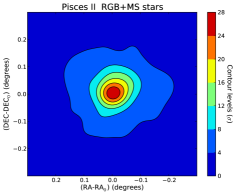
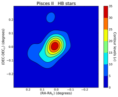
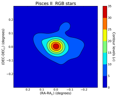
Figure 11: Isodensity contour maps of Psc II obtained with a bin size of 0.23^′. Left: Isodensity map of MS and RGB stars, selected with the guidance of the theoretical isochrones. Center: Same as in the left panel but for HB stars. Right: Same as in the left and middle panels but for RGB stars only. Peg III is located in the bottom-right direction on these maps. The colorbar provides the number of $\sigma$s above the background represented by each isodensity contour level. The isodensity contour levels in the maps of Psc II vary from 4 to 35 $\sigma$ above the background.

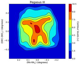
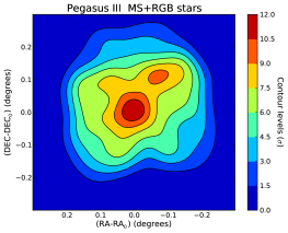
Figure 12: Isodensity contour maps of Peg III obtained with a bin size of 0.23^′. Left: Isodensity map from all stars in the photometric catalog of Peg III selected by $\chi$ and Sharpness parameters. Right panel: Same as in the left panel but only for MS and RGB stars selected with the guidance of the theoretical isochrones. Psc II is located in the top-left direction on these maps. The colorbar provides the number of $\sigma$s above the background represented by each isodensity contour level. The isodensity contour levels in the maps of Peg III vary from 1.5 to 12 $\sigma$ above the background.

Figure 11 shows the isodensity contour maps obtained from all stars in our photometric catalog of Psc II, selected by the $\chi$ and $Sharpness$ conditions described in Section 8 and using the same limits as for the galaxy CMD. The selected stars have been binned adopting a bin size of 0.23 arcmin. The left panel shows the isodensity contour map obtained selecting only MS and RGB stars (1387 sources), the center panel only HB stars (24 sources) and the right panel only RGB stars (309 sources). RGB, MS and HB stars were selected with the guidance of the theoretical isochrones we have overlaid on the galaxy CMD and, to minimize the contamination by field sources we considered only stars within 0.1 mag from the best fitting isochrones. To quantify a possible contamination of our subsamples by MW stars, on the assumption that the MW stars are uniformly distributed over the whole LBT FoV, we have counted the number of sources in 1 arcmin² regions at about 10 arcmin in distance from the centre of Psc II ($\gtrsim$ 10 $r_{h}$). This number corresponds to 6 sources, on average, which we can assume are all background/foreground objects. Since within an area of 1 arcmin² centered on Psc II we find 54 sources, we can conclude that at most $\sim$ 11 $\%$ of the sources in our subsamples may be MW contaminants. On the other hand, since the MW stars dominate the reddest part of the CMD ($B-V\geqslant$ 1.6 mag, see Fig 8), and barely overlaps with the Psc II RGB, MS and HB stars, we can safely assume that background/foreground contamination is almost negligible in the isodensity contour maps in Figure 11.

All maps in Figure 11 confirm the presence of a stellar overdensity at their center, corresponding to the position of the Psc II galaxy. This overdensity is clearly seen also in the isodensities of the RGB only and HB only stars. The isodensity maps of Psc II do not show an irregular shape as one would expect if the galaxy was undergoing tidal disruption or was interacting with Peg III. For sake of completeness, Peg III is located in the bottom-right direction on these maps.

Figure 12 shows the isodensity contour maps of Peg III obtained using the same bin size and selection of the sources by $\chi$ and $Sharpness$, as adopted for Psc II. The left panel corresponds to sources on the whole CMD (6557 stars) whereas the right panel corresponds to only MS+RGB stars selected by overlying the theoretical isochrones on the CMD of Peg III (1125 sources). Both isodensity maps show an overdensity at the center, corresponding to the Peg III galaxy. Other more extended overdensities are visible in the maps in Figure 12. They are not real structures but rather artefacts caused by regions with deeper exposures (see Fig. 4) due to the LBT rotation discussed in Sect. 3. The main overdensity at the center of the map on the left panel of Figure 12 is clearly seen also in the isodensity map of the RGB and MS stars, while the fictitious overdensities have now almost disappeared. Similarly to Psc II, the isodensity maps of Peg III do not show an irregular shape. The regular shape of the Psc II and Peg III isodensity maps leads us to rule out the existence of a clear link or stellar stream between these two UFDs.

11 Conclusions

Using $B$, $V$ time series photometry obtained with the LBCs at the LBT we have performed the first study of the variable stars in the Psc II and Peg III UFDs and derived the main properties of their resolved stellar populations. We have focused on the comparison of the Psc II and Peg III properties, in order to investigate the existence of a physical connection between these two galaxies which have a spatial separation of only 43 $\pm$ 19 kpc, as it was suggested in previous studies (Kim et al., 2015, 2016). For this comparison we have used as main tools (i) the properties of the RRLs identified in the two systems, (ii) the features of the observed CMDs and, (iii) the density contour maps.

In Psc II we have identified 4 variable stars (upper portion of Table 5): an RRab star (V1) with P $\sim$ 0.56 d, an SX Phoenicis star (V3; P $\sim$ 0.06 d) both lying within the r_h of Psc II, and a third variable, V4, with uncertain classification and about 0.25 mag brighter than V1, which is outside the galaxy’s r_h. A forth source within the r_h, V2, shows variability only in the $B$ band with P$\sim$0.05 d and was classified as candidate SX Phoenicis star. The period and amplitude of the light variation place V1 on the Oo I locus of the period–amplitude diagram. From the mean magnitude of V1 we measured a distance modulus: 21.22 $\pm$ 0.14 mag, that places Psc II at 175 $\pm$ 11 kpc from us, in agreement, within the errors, with previous literature estimates and at the same distance of Peg III. The period of V4 is uncertain. The source could either be an RRab star with P = 0.72 d or a first overtone AC with P = 0.42 d. However, from the comparison with theoretical isochrones overlaid on the galaxy CMD, and the $PL$ and $PW$ relations for ACs and CCs in the LMC, we conclude that V4 is likely a metal poor ([Fe/H] $\gtrsim$ $-$2.4 dex) RRab star with Oo II pulsation characteristics belonging to Psc II. The CMD suggests the presence in Psc II of a dominant old stellar population (t $>$ 10 Gyr) with metallicity [Fe/H] $>-$1.8 dex, along with, possibly, a minor, more metal poor component traced by Psc II-V4.

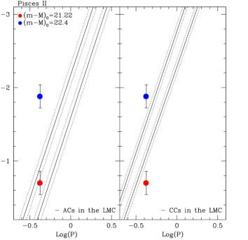
Figure 13: $PW$ relations (solid lines) for ACs (left panel; from Ripepi et al. 2014) and CCs (right panel; from Jacyszyn-Dobrzeniecka et al. 2016) in the LMC, transformed to the $B$ and $V$ bands. Dotted lines represent the 1$\sigma$ uncertainties, which for the AC relations correspond to 0.15 mag and for the CCs to 0.10 mag. A red filled circle shows the position of V4, according to the period of $\sim$ 0.42 d and a Wesenheit index calculated for a distance modulus of $(m-M)_{0}$ = 21.22 mag as estimated from V1, the RRL inside the half-light radius of Psc II. The blue filled circle show V4 but adopting a mass of 1.8M_⨀ and a Wesenheit index calculated for a distance modulus of 22.4 mag.

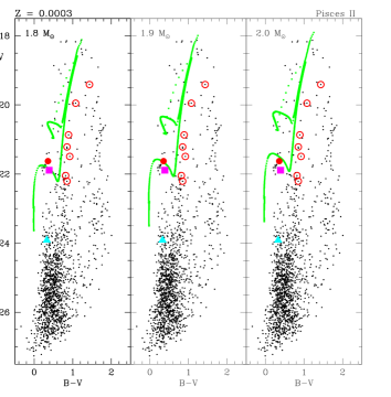
Figure 14: Stellar evolutionary tracks (BaSTI web interface) for 1.8, 1.9 and 2.0 M_⨀ (green solid line; left, central and right panels, respectively) and metallicity Z = 0.0003 ([Fe/H] = $-$1.8 dex) overlaid on the CMD of Psc II. The tracks were corrected adopting the distance modulus of Psc II derived from the RRab star [V1; $(m-M)_{0}$ =21.22 mag] and the reddening E($B-V$)=0.056 from Schlafly & Finkbeiner (2011) maps. V1 is marked by a magenta filled square, the AC/RRab star (V4) by a filled red circle, the SX Phe star (V3) by a cyan triangle and the spectroscopically confirmed members from Kirby et al. (2015) by red open circles.

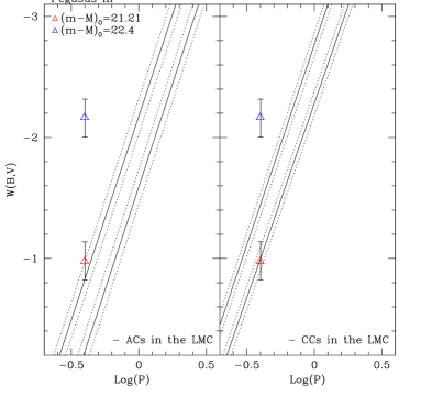
Figure 15: Same as in Fig. 13 but for the variable star with uncertain type classification in Peg III, star V2. A red triangle shows the position of V2, according to the period as AC (0.40 d) and a Wesenheit index calculated for a distance modulus of $(m-M)_{0}$ = 21.21 mag, as inferred from V1, the bona fide RRab star in Peg III. The blue triangle shows V2 but adopting a mass of 1.8 M_⨀ and a Wesenheit index calculated for a distance modulus of 22.4 mag.

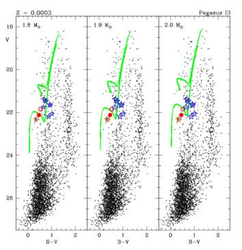
Figure 16: Stellar evolutionary tracks (BaSTI web interface) for 1.8, 1.9 and 2.0 M_⨀ (green solid line; left, central and right panels, respectively) and metallicity Z = 0.0003 ([Fe/H] = $-$1.8 dex) overlaid on the CMD of Peg III. The tracks were corrected adopting the distance modulus of Peg III derived from the RRab star [V1; $(m-M)_{0}$ =21.21 mag] and the reddening E($B-V$)=0.13 from Schlafly & Finkbeiner (2011) maps. V2 is marked by a red open circle, the bona-fide RRab star V1 by a red filled circle and the spectroscopically confirmed members from Kim et al. (2016) by blue and orange stars.

In Peg III we have identified 2 variable stars (lower portion of Table 5): an RRab star with P $\sim$ 0.55 days (V1) and a variable with uncertain type classification (V2). Both variables are located outside the galaxy r_h, respectively within 4r_h and 10r_h from the center of Peg III. Similarly to Psc II the period and amplitude of the bona-fide RRab star (V1) place the variable star close to the Oo I locus in the period–amplitude diagram (Figure 5). According to the distance modulus inferred from V1, 21.21 $\pm$ 0.23 mag, Peg III is at 174 $\pm$ 18 kpc, in good agreement with the literature and at the same distance from us as Psc II. V2 in Peg III has totally similar characteristic as V4 in Psc II. It could either be an RRab star with P $\sim$ 0.66 d or an AC with P $\sim$ 0.40 d and about 0.3 mag brighter than the galaxy HB. However, similar tests as done for Psc II-V4, lead us to conclude that V2 is very likely an RRab star with Oo II characteristics belonging to Peg III.

The comparison of the CMD with stellar isochrones suggests the presence also in Peg III of a dominant old stellar component ($>$ 10 Gyr) with metallicity larger than [Fe/H] $\sim-$1.8 dex. However, the RGB of Peg III exhibits a non negligible spread in color, indicative of a significant metallicity spread. This evidence, along with the pulsation properties of V2, indicate the presence in Peg III of an old, more metal-poor ([Fe/H] $\sim-$ 2.4 dex) stellar component, as also supported by the comparison with the mean ridge lines of Galactic GCs (see Fig. 10).

In summary, Psc II and Peg III not only share very similar properties but also almost same issues.

There are a number of alternative hypotheses that could explain why Psc II and Peg III have so much similar properties: 1) they could be the leftovers of a same large galaxy, which entered the MW environment and was totally disrupted by a close encounter with our Galaxy some Gyrs ago; 2) they could be satellites of one of the present day MW dSph satellites or of a dSph that has been completely cannibalized by the MW; 3) they could be separate entities, that just by chance are close on the sky and share similar properties; and, finally: 4) they could have been born in a pair. However, in spite of all the similarities and the proximity on the sky, the density contour maps do not reveal signatures of a tidal interaction between them. If they were indeed born in a pair, or were physically connected in the past, no trace of this physical connection seems to have survived.

The analysis we have presented here revealed very intriguing characteristics and similarities of Psc II and Peg III, prompting us to further study these systems. Unfortunately, the HB of the two galaxies is at/below the limiting magnitude reached by Gaia ($V\sim$ 20.5-21 mag; Gaia Collaboration et al. 2018); but their brighter RGB stars are well within the reach of Gaia. Psc II and Peg III are in a region of the sky still poorly sampled by the observations released in Gaia DR2. However, the Gaia sky coverage is rapidly increasing and in future data releases Gaia will likely tell us whether Psc II and Peg III share the same relative proper motions. Furthermore, in the near future the Rubin Observatory Large Synoptic Survey Telescope (LSST), designed to collect deep (5 mag deeper than Gaia) ground-based, wide-field imaging from the blue to the near-infrared wavelengths, will be able to provide observations of Psc II and Peg III and the field between them deep enough to shed light on the nature and origin of these intriguing couple.

Appendix A Psc II-V4 and Peg III-V2 as Anomalous Cepheids

ACs are known to follow specific Period-Lumiosity ($PL$) and Period-Wesenheit ($PW$) relations, which differ from both the classical and the Type II Cepheids relationships (Soszyński et al., 2008). Therefore, if V4 and V2 are ACs, they should conform to the $PL$ and $PW$ relations of ACs.

We have compared V4 with the $PW$ relations followed by ACs in the Large Magellanic Cloud (LMC; see Ripepi et al., 2014). These relations are defined in the $V$ and $I$ bands, hence we converted them to the $B$, $V$ bands using the relation $\langle W(V,I)\rangle=-0.22(\pm 0.001)+1.03\langle W(B,V)\rangle$ (Eq. 12 of Marconi et al. 2004).

The $PW$ relations of the LMC ACs converted into $B$ and $V$ bands are shown as solid lines in the left panel of the Fig. 13, together with their 1$\sigma$ uncertainties (dotted lines). In this figure the lower line is the $PW$ relation for fundamental mode ACs, while the upper line is for ACs that pulsate in the first-overtone mode. Psc II-V4 (red filled circle) is plotted according to the period as an AC and the Wesenheit index computed by correcting the star $\langle V\rangle$-band apparent magnitude for the distance modulus (m-M)₀ = 21.22 mag as estimated from V1, the RRab star within the r_h of Psc II. V4 lies within the 1$\sigma$ uncertainty of the $PW$ relation for first-overtone ACs, hence, it could indeed be an AC belonging to Psc II. As a check, in the right panel of Fig. 13 we have compared V4 also with the $PW$ relations for LMC Classical Cepheids (CCs) by Jacyszyn-Dobrzeniecka et al. (2016). The star appears to be significantly fainter than the Wesenheit index of a fundamental-mode CCs with same period, hence, it is unlikely that it could be a CC of Psc II. Furthermore, in the CMD of Psc II (see Fig. 8) there is no indication of the presence of a young population ($<$ 500 Myr) as that traced by CCs [for a detailed description of the Psc II CMD (and the Peg III CMD as well) we refer the reader to Section 8]. Figure 13 seems thus to support the possibility that V4 might be a first overtone AC of Psc II. We further checked this hypothesis comparing the star with stellar evolutionary tracks by Pietrinferni et al. (2004, available at http://basti.oa-teramo.inaf.it/index.html), for the typical mass and metallicity of ACs ($\sim$1.8-2.2 M_⨀ according to Caputo et al. 2004 and Z = 0.0004 following Marconi et al. 2004).

This is illustrated in the three panels of Fig. 14 that show the CMD of Psc II with overlaid evolutionary tracks for metallicity Z = 0.0003 and masses of 1.8, 1.9 and 2.0 M_⨀, corrected for the distance modulus of Psc II and for a reddening of E($B-V$) = 0.056 mag according to Schlafly & Finkbeiner (2011).

This comparison shows that if V4 were indeed an AC belonging to Psc II it should be at least 1 mag brighter to lie on the proper region of the evolutionary track: the hook above the HB. On the other hand, since V4 is at about five r_h from the Psc II center, it could be a field AC. We thus shifted the stellar tracks as to fit the luminosity of V4 and found that the hook of the 1.8 M_⨀ track would fit the luminosity of V4 for a distance modulus of $(m-M)_{0}$ $\sim$ 22.4 mag and for longer moduli in case of larger masses.

However, adopting such longer distance moduli, V4 could no longer fit any of the $PW$ relations for ACs or CCs, as clearly shown by blue filled circles in Fig. 13. Based on these conflicting results we conclude that the classification of V4 as an AC either belonging to Psc II or to the background field is very unlikely. Totally similar conflicting results were found also for V2 in Peg III (see Figs. 15 and 16), leading us to rule out a classification as AC also for V2 in Peg III.

Appendix B DOTTER et AL. 2008 ISOCHRONES ON THE CMD of Psc II

Figure 17 shows CMD of Psc II (same as left panel of Fig 8) with overlaid Dotter et al. (2008)’s isochrones for different metallicities, $-$2.5, $-$2.0 and $-$1.5 dex, a fixed age (13.5 Gyr left panels; 11Gyr right panels) and a fixed [$\alpha$/Fe] enhancement of 0.2 dex in fig A and 0.6 dex in fig. B. The best agreement between variable stars and spectroscopic metal-poor stars is achieved for an isochrone with metal abundance between $-$2 and $-$1.5 dex and rather old. Here, Dotter et al. (2008) isochrones with 13.5 Gyr seem to be quite consistent with the PARSEC isochrones of 13 Gyr we have used throughout the paper. In summary, results do not seem to change significantly changing the isochrone set adopted as reference. On the other hand, the discrepancy with previous studies may also arise because the photometry in this paper is much deeper than previous works.

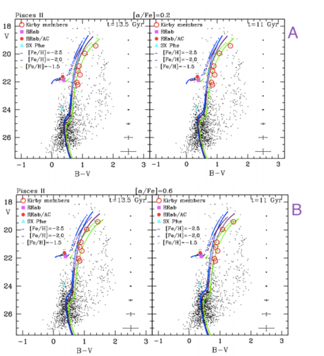
Figure 17: Same as left panel of Fig 8 with overlaid Dotter et al. (2008)’s isochrones for different metallicities (from $-$2.5 to $-$1.5 dex), a fixed age (13.5 Gyr left panels; 11 Gyr right panels) and a fixed [$\alpha$/Fe] enhancement of 0.2 dex (fig. A) and 0.6 dex (fig. B).

References

- Ahn et al. (2014) Ahn, C. P., Alexandroff, R., Allende Prieto, C., et al. 2014, ApJS, 211, 17
- Aihara, et al. (2018) Aihara H., et al., 2018, PASJ, 70, S4
- Alcock et al. (2000) Alcock, C., Allsman, R. A., Alves, D. R. et al. 2000, AJ, 119, 2194
- Arellano Ferro et al. (2018) Arellano Ferro, A., Rojas Galindo, F. C., Muneer, S., & Giridhar, S. 2018, Rev.
- Arenou et al. (2018) Arenou, F., Luri, X., Babusiaux, C., et al. 2018, A&A, 616, A17
- Bailey (1902) Bailey, S. I. 1902, Annals of Harvard College Observatory, 38, 1
- Bailey & Pickering (1913) Bailey, S. I., & Pickering, E. C. 1913, Annals of Harvard College Observatory, 78, 1
- Bailey et al. (1919) Bailey, S. I., Leland, E. F., Woods, I. E., & Pickering, E. C. 1919, Annals of Harvard College Observatory, 78, 195
- Belokurov et al. (2007) Belokurov, V., Zucker, D. B., Evans, N. W., et al. 2007, ApJ, 654, 897
- Belokurov et al. (2010) Belokurov, V., Walker, M. G., Evans, N. W., et al. 2010, ApJ, 712, L103
- Bernard et al. (2014) Bernard, E. J., Ferguson, A. M. N., Schlafly, E. F., et al. 2014, MNRAS, 442, 2999
- Bland-Hawthorn et al. (2015) Bland-Hawthorn, J., Sutherland, R., & Webster, D. 2015, ApJ, 807, 154. doi:10.1088/0004-637X/807/2/154
- Boettcher et al. (2013) Boettcher, E., Willman, B., Fadely, R., et al. 2013, AJ, 146, 94
- Bovill & Ricotti (2009) Bovill M. S., Ricotti M., 2009, ApJ, 693, 1859
- Bressan et al. (2012) Bressan, A., Marigo, P., Girardi, et al. 2012, MNRAS, 427, 127
- Bruzual & Charlot (2003) Bruzual, G., & Charlot, S. 2003, MNRAS, 344, 1000
- Bullock & Johnston (2005) Bullock, J. S., & Johnston, K. V. 2005, ApJ, 635, 931
- Cacciari et al. (2005) Cacciari, C., Corwin, T. M., & Carney, B. W. 2005, AJ, 129, 267
- Calura, et al. (2015) Calura F., Few C. G., Romano D., D’Ercole A., 2015, ApJL, 814, L14
- Caputo et al. (2004) Caputo, F., Castellani, V., Degl’Innocenti, S., Fiorentino, G., & Marconi, M. 2004, A&A, 424, 927
- Chambers et al. (2016) Chambers, K. C., Magnier, E. A., Metcalfe, N., et al. 2016, arXiv:1612.05560
- Clement & Rowe (2000) Clement, C. M., & Rowe, J. 2000, AJ, 120, 2579
- Clementini et al. (2000) Clementini, G., Di Tomaso, S., Di Fabrizio, L., et al. 2000, AJ, 120, 2054
- Clementini et al. (2003) Clementini, G., Gratton, R. G., Bragaglia, A., et al. 2003, AJ, 125, 1309
- Clementini (2010) Clementini, G. 2010, in Variable Stars, the Galactic halo and Galaxy Formation, ed. C. Sterken, N. Samus, & L. Szabados (Moscow: Sternberg Astronomical Institute of Moscow Univ.), 107
- Clementini et al. (2012) Clementini, G., Cignoni, M., Contreras Ramos, R., et al. 2012, ApJ, 756, 108
- Clementini et al. (2016) Clementini, G., Ripepi, V., Leccia, S., et al. 2016, A&A, 595, A133
- Clementini et al. (2019) Clementini, G., Ripepi, V., Molinaro, R., et al. 2019, A&A, 622, A60
- Dall’Ora et al. (2006) Dall’Ora, M., Clementini, G., Kinemuchi, K., et al. 2006, ApJ, 653, L109
- Dall’Ora et al. (2012) Dall’Ora, M., Kinemuchi, K., Ripepi, V., et al. 2012, ApJ, 752, 42
- de Jong et al. (2010) de Jong, J. T. A., Martin, N. F., Rix, H.-W., et al. 2010, ApJ, 710, 1664
- Dotter et al. (2007) Dotter, A., Chaboyer, B., Jevremović, D., et al. 2007, AJ, 134, 376. doi:10.1086/517915
- Dotter et al. (2008) Dotter, A., Chaboyer, B., Jevremović, D., et al. 2008, ApJS, 178, 89
- Drake et al. (2014) Drake, A. J., Graham, M. J., Djorgovski, S. G., et al. 2014, ApJS, 213, 9
- Drlica-Wagner et al. (2015) Drlica-Wagner, A., Bechtol, K., Rykoff, E. S., et al. 2015, ApJ, 813, 109
- Gaia Collaboration et al. (2018) Gaia Collaboration, Brown, A. G. A., Vallenari, A., et al. 2018, A&A, 616, A1
- Garling et al. (2018) Garling, C., Willman, B., Sand, D. J., et al. 2018, ApJ, 852, 44
- Garofalo et al. (2013) Garofalo, A., Cusano, F., Clementini, G., et al. 2013, ApJ, 767, 62
- Gautschy & Saio (2017) Gautschy, A. & Saio, H. 2017, MNRAS, 468, 4419
- Giallongo et al. (2008) Giallongo, E., Ragazzoni, R., Grazian, A., et al., 2008, A&A 482,349
- Girardi et al. (2004) Girardi, L., Grebel, E. K., Odenkirchen, M., & Chiosi, C. 2004, A&A, 422, 205
- Gratton et al. (2004) Gratton, R. G., Bragaglia, A., Clementini, G., et al. 2004, A&A, 421, 937
- Greco et al. (2008) Greco, C., Dall’Ora, M., Clementini, G., et al. 2008, ApJ, 675, L73
- Harris (1996) Harris, W. E. 1996, AJ, 112, 1487
- Homma, et al. (2019) Homma D., et al., 2019, PASJ..tmp, 91
- Jacyszyn-Dobrzeniecka et al. (2016) Jacyszyn-Dobrzeniecka, A. M., Skowron, D. M., Mróz, P., et al. 2016, Acta Astronomica, 66, 149
- Joo et al. (2019) Joo S.-J., et al., 2019, ApJ, 875, 120
- Jurcsik & Kovacs (1996) Jurcsik, J., & Kovacs, G. 1996, A&A, 312, 111
- Kim et al. (2015) Kim, D., Jerjen, H., Mackey, D., Da Costa, G. S., & Milone, A. P. 2015, ApJ, 804, L44
- Kim et al. (2016) Kim, D., Jerjen, H., Geha, M., et al. 2016, ApJ, 833, 16
- Kirby et al. (2008) Kirby, E. N., Simon, J. D., Geha, M., Guhathakurta, P., & Frebel, A. 2008, ApJ, 685, L43
- Kirby, et al. (2013) Kirby E. N., Cohen J. G., Guhathakurta P., Cheng L., Bullock J. S., Gallazzi A., 2013, ApJ, 779, 102
- Kirby et al. (2015) Kirby, E. N., Simon, J. D., & Cohen, J. G. 2015, ApJ, 810, 56
- Koposov, et al. (2015) Koposov S. E., et al., 2015, ApJ, 811, 62
- Koposov et al. (2018) Koposov, S. E., Walker, M. G., Belokurov, V., et al. 2018, MNRAS, 479, 5343
- Kuehn et al. (2008) Kuehn, C., Kinemuchi, K., Ripepi, V., et al. 2008, ApJ, 674, L81
- Laevens et al. (2015) Laevens, B. P. M., Martin, N. F., Bernard, E. J., et al. 2015, ApJ, 813, 44
- Lee et al. (1990) Lee, Y.-W., Demarque, P., & Zinn, R. 1990, ApJ, 350, 155
- Li et al. (2018) Li, T. S., Simon, J. D., Pace, A. B., et al. 2018, ApJ, 857, 145. doi:10.3847/1538-4357/aab666
- Lindegren et al. (2018) Lindegren, L., Hernández, J., Bombrun, A., et al. 2018, A&A, 616, A2
- Lomb (1976) Lomb, N. R. 1976, Ap&SS, 39, 447
- Madore (1982) Madore, B. F. 1982, ApJ, 253, 575
- Maguire (2017) Maguire K., 2017, hsn..book, 293, hsn..book
- Marconi et al. (2004) Marconi, M., Fiorentino, G., & Caputo, F. 2004, A&A, 417, 1101
- Marconi, et al. (2006) Marconi M., Cignoni M., Di Criscienzo M., Ripepi V., Castelli F., Musella I., Ruoppo A., 2006, MNRAS, 371, 1503
- Martin et al. (2008) Martin, N. F., de Jong, J. T. A., & Rix, H.-W. 2008, ApJ, 684, 1075
- Martínez-Vázquez et al. (2019) Martínez-Vázquez, C. E., Vivas, A. K., Gurevich, M., et al. 2019, MNRAS, 490, 2183
- Mateo (1998) Mateo, M. L. 1998, Annual Review of A&A, 36, 435
- Medina et al. (2017) Medina, G. E., Muñoz, R. R., Vivas, A. K., et al. 2017, ApJ, 845, L10
- Medina et al. (2018) Medina G. E., et al., 2018, ApJ, 855, 43
- Moretti et al. (2009) Moretti, M. I., Dall’Ora, M., Ripepi, V., et al. 2009, ApJ, 699, L125
- Mori, Ferrara & Madau (2002) Mori M., Ferrara A., Madau P., 2002, ApJ, 571, 40
- Muñoz et al. (2010) Muñoz, R. R., Geha, M., & Willman, B. 2010, AJ, 140, 138. doi:10.1088/0004-6256/140/1/138
- Muraveva et al. (2018) Muraveva, T., Delgado, H. E., Clementini, G., et al. 2018, MNRAS, 481, 1195
- Musella et al. (2009) Musella, I., Ripepi, V., Clementini, G., et al. 2009, ApJ, 695, L83
- Musella et al. (2012) Musella, I., Ripepi, V., Marconi, M., et al. 2012, ApJ, 756, 121
- Nath & Shchekinov (2013) Nath B. B., Shchekinov Y., 2013, ApJL, 777, L12
- Norris et al. (2010) Norris, J. E., Wyse, R. F. G., Gilmore, G., et al. 2010, ApJ, 723, 1632
- Oosterhoff (1939) Oosterhoff, P. T. 1939, The Observatory, 62, 104
- Piersimoni et al. (2002) Piersimoni, A. M., Bono, G., & Ripepi, V. 2002, AJ, 124, 1528
- Pietrinferni et al. (2004) Pietrinferni, A., Cassisi, S., Salaris, M., & Castelli, F. 2004, ApJ, 612, 168
- Piotto et al. (2002) Piotto, G., King, I. R., Djorgovski, S. G., et al. 2002, A&A, 391, 945
- Renzini, et al. (2015) Renzini A., et al., 2015, MNRAS, 454, 4197
- Ripepi et al. (2014) Ripepi, V., Marconi, M., Moretti, M. I., et al. 2014, MNRAS, 437, 2307
- Romano et al. (2015) Romano, D., Bellazzini, M., Starkenburg, E., et al. 2015, MNRAS, 446, 4220. doi:10.1093/mnras/stu2427
- Romano et al. (2019) Romano, D., Calura, F., D’Ercole, A., et al. 2019, A&A, 630, A140
- Salpeter (1955) Salpeter E. E., 1955, ApJ, 121, 161
- Sand et al. (2012) Sand, D. J., Strader, J., Willman, B., et al. 2012, ApJ, 756, 79
- Sales et al. (2007) Sales, L. V., Navarro, J. F., Abadi, M. G., & Steinmetz, M. 2007, MNRAS, 379, 1464
- Salvadori & Ferrara (2009) Salvadori S., Ferrara A., 2009, MNRAS, 395, L6
- Scargle (1982) Scargle, J. D. 1982, ApJ, 263, 835
- Schlafly & Finkbeiner (2011) Schlafly, E. F., & Finkbeiner, D. P. 2011, ApJ, 737, 103
- Sesar et al. (2014) Sesar, B., Banholzer, S. R., Cohen, J. G., et al. 2014, ApJ, 793, 135
- Shanks et al. (2015) Shanks, T., Metcalfe, N., Chehade, B., et al. 2015, MNRAS, 451, 4238
- Siegel et al. (2008) Siegel, M. H., Shetrone, M. D., & Irwin, M. 2008, AJ, 135, 2084. doi:10.1088/0004-6256/135/6/2084
- Silich & Tenorio-Tagle (2018) Silich S., Tenorio-Tagle G., 2018, MNRAS, 478, 5112
- Simon & Geha (2007) Simon, J. D., & Geha, M. 2007, ApJ, 670, 313
- Simon et al. (2011) Simon, J. D., Geha, M., Minor, Q. E., et al. 2011, ApJ, 733, 46
- Soszyński et al. (2008) Soszyński, I., Udalski, A., Szymański, M. K., et al. 2008, Acta Astronomica, 58, 293
- Simon (2019) Simon, J. D. 2019, ARA&A, 57, 37
- Stetson (1987) Stetson, P. B. 1987, PASP, 99, 191
- Stetson (1994) Stetson, P. B. 1994, PASP, 106, 250
- Stierwalt et al. (2017) Stierwalt, S., Liss, S. E., Johnson, K. E., et al. 2017, Nature Astronomy, 1, 0025
- Strigari et al. (2008) Strigari, L. E., Koushiappas, S. M., Bullock, J. S., et al. 2008, ApJ, 678, 614
- The Dark Energy Survey Collaboration (2005) The Dark Energy Survey Collaboration 2005, arXiv:astro-ph/0510346
- Tolstoy et al. (2009) Tolstoy, E., Hill, V., & Tosi, M. 2009, ARA&A, 47, 371
- Torrealba et al. (2016) Torrealba, G., Koposov, S. E., Belokurov, V., & Irwin, M. 2016, MNRAS, 459, 2370
- Torrealba et al. (2018) Torrealba, G., Belokurov, V., Koposov, S. E., et al. 2018, MNRAS, 475, 5085
- VandenBerg et al. (2016) VandenBerg, D. A., Denissenkov, P. A., & Catelan, M. 2016, ApJ, 827, 2
- Vincenzo, et al. (2019) Vincenzo F., Spitoni E., Calura F., Matteucci F., Silva Aguirre V., Miglio A., Cescutti G., 2019, MNRAS, 487, L47
- Vivas et al. (2016) Vivas, A. K., Olsen, K., Blum, R., et al. 2016, AJ, 151, 118
- Vivas et al. (2020) Vivas, A. K., Martínez-Vázquez, C., & Walker, A. R. 2020, ApJS, 247, 35
- Walsh et al. (2007) Walsh, S. M., Jerjen, H., & Willman, B. 2007, ApJ, 662, L83
- Yanny et al. (2009) Yanny, B., Rockosi, C., Newberg, H. J., et al. 2009, AJ, 137, 4377
- Yadav, et al. (2017) Yadav N., Mukherjee D., Sharma P., Nath B. B., 2017, MNRAS, 465, 1720
- York et al. (2000) York, D. G., Adelman, J., Anderson, J. E., Jr., et al. 2000, AJ, 120, 1579
- Zorotovic et al. (2010) Zorotovic, M., Catelan, M., Smith, H. A., et al. 2010, AJ, 139, 357