On the stability of Rotating States in Second-Order Self-Propelled Multi-Particle Systems

Abstract.

The study of emergent behavior of swarms is of great interest for applied sciences. In this paper, we study the stability of the system of $n$-coupled self-propelled particle systems $\ddot{r}_{k}=(1-|\dot{r}_{k}|^{2})\dot{r}_{k}-\frac{1}{n}\sum_{m=1}^{n}(r_{k}-r_{m})$, $r_{k}\in\mathbb{R}^{2}$, with all-to-all spring-like coupling. Previous numerical experiments have shown that for a large set of initial conditions, after an initial drift, the center of mass of the system converges to a stationary point and each particle eventually rotates with unit angular velocity around the stationary center of mass. The distribution of the particles on the circle need not be uniform. Such limit states are dubbed rotating states. We prove that a rotating state with particles spinning in the same direction is stable and we show that every solution that starts near a rotating state asymptotically approaches a rotating state. The proof uses new slow manifold ideas to improve the approximations of the flow on the center manifold in the presence of non-isolated fixed points.

1. Introduction

The onset of synchronization or, more generally, emergence of collective patterns in multi-agent systems is a well-documented phenomenon spanning many applied and theoretical disciplines [19, 20]. The description of limit states of a given system and the stability analysis of these states are some of the most important questions in the field.

This note is devoted to the study of a second-order system of $n$ particles swarming in the plane in which every agent accelerates based on a nonlinear function of its velocity and a linear attraction to the center of mass, i.e. an all-to-all coupled network of agents with self-propulsion. The equations governing the system are:

$$\begin{split}\ddot{r}_{k}&=(1-|\dot{r}_{k}|^{2})\dot{r}_{k}-\frac{1}{n}\sum_{m=1}^{n}(r_{k}-r_{m}).\end{split}$$ (1)

or, equivalently,

$$\begin{split}\ddot{r}_{k}&=(1-|\dot{r}_{k}|^{2})\dot{r}_{k}-(r_{k}-R)\end{split}$$ (2)

where $R=\frac{1}{n}\sum_{j=1}^{n}r_{m}$ is the center of mass of the system. Here, $r_{k}=(x_{k},y_{k})$ represents the two-dimensional position vector of the $k$-th particle and $\dot{r}_{k}$ stands for the time derivative $\frac{dr_{k}}{dt}$. We refer the reader to [16, 22, 6] for various applications of System (1).

Mathematical models of multi-agents whose dynamics is very simple if acting in isolation, but develop complex patterns or structures when coupled, go as far back as 1951 [23, Turing]. The earlier models stem from the field of cellular biology; their coupling is linear, quantifying the diffusion of various morphogens or enzymes past the membranes of neighboring cells [23, 21]. These models highlight a paradoxical aspect in the evolution of multi-agent dynamical systems: otherwise “dead” cells (i.e. convergent to a stable fixed point, [21]) turn alive (pulsating or oscillating) due to their interactions. Similarly, despite its seeming simplicity, System (1) exhibits a very complex behavior that is heavily dependent on the initial conditions. This point will be repeatedly illustrated and highlighted throughout the introduction.

If in Equation (1) the agents are isolated from each other, the equation of motion for each individual agent becomes

$$\ddot{r}_{k}=(1-|\dot{r}_{k}|^{2})\dot{r}_{k}.$$

Consider the velocity of one isolated particle $v_{k}=\dot{r}_{k}$. The direction of motion for each particle with nonzero initial velocity stays unchanged, along $\dot{r}_{k}(0);$ since $|v_{k}|^{2}$ satisfies the logistic equation $\frac{d}{dt}{(|v_{k}|^{2})}=2|v_{k}|^{2}(1-|v_{k}|^{2})$, the speed $|v_{k}|$ asymptotically approaches one. In isolation, the agents diverge away from the origin on $n$ lines, not necessarily distinct.

Introducing coupling into (1) fundamentally alters the dynamics of the system: regardless of the initial conditions, the agents remain in a spatially cohesive configuration around the center of mass [17], meaning that the deviations of particles from the center of mass, $r_{k}-R$, and their velocities $\dot{r}_{k}$ are eventually bounded by a constant that depends only on the number of particles. If the center of mass escapes to infinity ($|R|$ can only increase linearly in time [17]), then all agents (and the center of mass) synchronize their directions of motion. If the center of mass remains bounded, then the agents exhibit oscillatory patterns.

In what follows, it will be convenient to identify the points in $\mathbb{R}^{2}$ with complex numbers. We will use the Roman typestyle for complex numbers $\mathrm{r}=x+iy$ and the regular math font for the corresponding vectors $r=(x,y)$.

Numerical simulations have captured a range of limit behaviors for the $4n$-dimensional system (1), including circular configurations in which the agents eventually rotate around some point $R_{0}\in\mathbb{R}^{2}$, a stationary center of mass: $\mathrm{r}_{k}(t)=e^{\pm it+i\theta_{0,k}}+\mathrm{R}_{0}$ (Figure 1), and perturbations of the linear motion with unit speed, $r_{k}(t)=v_{0}t+d$, $v_{0},d\in\mathbb{R}^{2}$ (Figure 2). These states have been conjectured to be stable, but except for the case of $n=2$ agents, results are lacking. The main difficulties in the analysis of these states are associated with the large dimensionality of the central manifold, the large number of parameters codifying the states, and the fact that the states are non-isolated, even after factoring out the rotation and translation invariance.

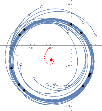
Figure 1. Asymptotic behavior of (1) in the basin of attraction of a non-degenerate rotating state for $t\in[0,18]$. The center of mass $R(t)$ at $t=18$ is indicated as a red dot. The dashed line represents the trajectory of $R(t)$. The positions of the agents at $t=0$ (at $t=18$) are represented as hollow (solid) dots. Agents eventually rotate around the circle of radius 1 centered at $R(t)$ at a constant speed of 1, as the center of mass becomes stationary. In rotating states, the polar angles $\{\theta_{k}\}$ of the agents about the center of mass satisfy $\sum_{k=1}^{n}e^{i\theta_{k}}=0$.

We call the circular limit cycles rotating states if all agents rotate in the same direction about the stationary center of mass. In this paper we only discuss the case of counterclockwise motion $\mathrm{r}_{k}(t)=e^{it+i\theta_{0,k}}+\mathrm{R}_{0}$; clockwise motion follows as the system is symmetric with respect to reflection over the $x$-axis. We call configurations where all $r_{k}$ have identical linear solutions, $r_{k}(t)=v_{0}t+d$, translating states. Note that we eschew the more familiar names of “mills” and “flocks” since their usage is inconsistent among authors: some authors, but not all, require that particles in a mill or flock be uniformly distributed about the center of mass. We want to emphasize that we make no symmetry or uniform-distribution assumptions. In fact, a considerable portion of the paper is dedicated to studying the degenerate configurations when the agents split into two equally-sized clumps. In that case, the customary Taylor approximations for the central manifold fail to capture the dynamics, no matter how high the degree. To address that, we designed a novel technique for approximating the central manifold, one that is consistent with scales of the flow and that works very well in the presence of non-isolated fixed points, and applied to the system at hand. The reader interested in learning in how to apply it to a larger class of systems can refer to Appendix where the general framework for approximating center manifolds around non-isolated fixed points is presented.

The main result of the paper is a rigorous proof of the stability of rotating states of (1), which establishes the mathematical foundation for the observations made in numerical simulations.

Theorem 1.1.

Every rotating state solution of Equation (1) is stable. Furthermore, every solution that starts near a rotating state converges to a nearby rotating state.

More specifically, we show that for any $\epsilon>0$ there exists $\delta>0$ such that given any initial center of mass location $\mathrm{R}_{0}$ and polar angles $\theta_{0,k}$ with $\sum_{k=1}^{n}e^{i\theta_{0,k}}=0$, if a solution $\{\mathrm{r}_{k}(t)\}$ of (1) satisfies $|\mathrm{r}_{k}(0)-e^{i\theta_{0,k}}|<\delta$ and $|\dot{\mathrm{r}}_{k}(0)-ie^{i\theta_{0,k}}|<\delta$, then

$$|\mathrm{r}_{k}(t)-(\mathrm{R}_{0}+e^{i\theta_{0,k}}e^{it})|<\epsilon\mbox{ and }|\dot{r}_{k}(t)-ie^{i\theta_{0,k}}e^{it}|<\epsilon\mbox{ for all }t\geq 0.$$

Furthermore, there exist $\mathrm{R}_{\infty}$ and $\theta_{\infty,k}$ with $\sum_{k=1}^{n}e^{i\theta_{\infty,k}}=0$ such that

$$\lim_{t\to\infty}\left[\mathrm{r}_{k}(t)-(\mathrm{R}_{\infty}+e^{i\theta_{\infty,k}}e^{it}))\right]=0\mbox{ and }\lim_{t\to\infty}\left[\dot{\mathrm{r}}_{k}(t)-ie^{i\theta_{\infty,k}}e^{it}\right]=0.$$

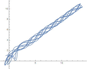
Figure 2. Translating state behavior of ten agents with random initial positions in the square $[-1,1]\times[-1,1]$ and random initial velocities drawn from the square $[0,1]\times[0,1]$. The curves represent the agents’ trajectories.

System (1) can be viewed as belonging to the class of second-order gradient-like systems $\ddot{r}=f(\dot{r})-\nabla U(r)$. However, the existing theory – see, for example, [10, Ch. 7] and [9] – does not apply to (1). We note that the authors of [9] and [10, Ch. 7] showed that under some conditions on $f$ and the potential function $U$, most notably $f(\dot{r})\cdot\dot{r}<0$ if $\dot{r}\neq 0$, every bounded solution converges to a configuration that solves $\nabla U(r)=0$. Since the function $(1-|\dot{r}_{k}|^{2})\dot{r}_{k}\cdot\dot{r}_{k}$ in (1) is not negative-definite, the results of [9] do not apply.

An in-depth discussion of the existence of a global attractor and the synchronization of dissipative systems with strong coupling can be found in [8]. In Section 3 of [8], it is proven that 1-dimensional Duffing oscillators with a strong enough diffusive coupling (using nearest neighbor coupling) synchronize; exceeding a large threshold for the coupling is a necessary condition in [8].

If in Equation (1) we assume that the positions $r_{k}(t)$ and velocities $\dot{r}_{k}$ are collinear, that is, the motion takes place on a line, by switching to the velocity-acceleration coordinates, we obtain a system of coupled Van der Pol equations. Some classes of coupled Van der Pol equations have been shown to admit nontrivial periodic cycles [11].

If the planar agents in (1) maintain a stationary center of mass (referred to as a decoupled system), then their dynamics is described by the equation(s) $\ddot{r}_{k}=(1-|\dot{r}_{k}|^{2})\dot{r}_{k}-r_{k}$, belonging to the class of generalized Liénard systems. Furthermore, if the motion of the decoupled system is restricted to the $x$-axis (or to any other line through the origin), the stability properties of the solutions to $\ddot{x}-\dot{x}+(\dot{x})^{3}+x=0$ follow from the classic Liénard theorem [14], [24, Theorem 4.6]. In this 1-dimensional decoupled case, there exists a unique nontrivial periodic cycle, with approximate amplitude of 1.279 and period of 6.662 (note the larger amplitude and longer period compared to the rotating state, of amplitude 1 and period $2\pi$). Every other non-zero solution (with initial position $r(0)$ and velocity $\dot{r}(0)$ along the $x$-axis) approaches this cycle. The configuration of multiple agents in the plane with each agent pulsating along (its own) line through the center of mass, keeping a stationary center of mass, is unstable. The instability is triggered by perturbing the velocity off the initial line of motion.

The decoupled system when the initial position $r(0)$ and velocity $\dot{r}(0)$ are not collinear is discussed in Theorem 2.1, in which we show that that every non-zero solution of the decoupled system approaches one of the cycles $\mathrm{r}(t)=e^{\pm it}$.

In literature, oscillators are often compared to the Kuramoto oscillators. We note that unlike the Kuramoto oscillators, the interaction of the spatial angles $\tan^{-1}(y_{k}/x_{k})$, $r_{k}=(x_{k},y_{k})$, of particles governed by (1) is not just with each other, but is also influenced by the spatial proximity of variables $|r_{k}|$ and $|\dot{r}_{l}|$, making (1) a swarmalator per [19, 20]. Numerical and theoretical investigations of swarmalators with equally distributed phase angles and specific fast-decaying coupling can be found in [19, 20] and [18].

Another interesting feature of (1) is that for some configurations near rotating states (see Section 5) the rate of convergence of the center of mass to its limiting location is of the order $\frac{1}{\sqrt{t}}$, whereas for some other configurations the convergence is exponentially fast with the exponent depending on the “spread” of the particles. The presence of such features makes the stability analysis of (1) extremely difficult.

We also note that the limit behavior of flocks and rings whose particles are equally distributed on a circle (i.e. ring mills) have been numerically analyzed extensively, using both individual-based and continuum models, see, for example, [5], [13], [1] for self-propelled particles, and [12] for the steady state pattern formation. There are very few results that relax the equally-distributed assumption: [4] addresses the stability of flocks satisfying certain hyperbolicity assumptions, but for System (1) those assumptions are only satisfied for $n=2$ agents: more specifically, if $n\geq 3,$ the translating states and the rotating states of (1) have more neutral directions than what Condition H3 (“obvious symmetries”’) of [4] requires.

A brief outline of the paper follows. In Section 2 we introduce main definitions, give an overview of various limit configurations for System (1), and study stability properties of the decoupled system (Theorem 2.1).

The proof of Theorem 1.1 is divided into three parts which are presented in Sections 3, 4, and 5. In Section 3 we introduce a new coordinate system $\{X_{k},Y_{k}\}$ based on a rotating frame of reference, by setting $\mathrm{r}_{k}=e^{it}(X_{k}+iY_{k})$, and establish that the set of equilibrium points in this new coordinate system corresponds to the set of rotating states centered at the origin in the original coordinates.

In Section 4 we present the proof of Theorem 1.1 for the case of a non-degenerate rotating state, that is, a rotating state for which the family of vectors $r_{k}-R$, $k=1,\ldots,n$, is not collinear (collinearity within a rotating state can only happen for even $n$). For non-degenerate configurations we conduct spectral analysis (using the rotating frame Jacobian) to show that the center manifold has dimension $n$ for any non-degenerate rotating state configuration. We show that the spectral gap of the Jacobian decreases to zero as the initial configurations of the non-degenerate rings approach a degenerate one. To study the dynamics on the central manifold, we eschew the traditional approach of approximating the central manifold (and its flow) by Taylor polynomials in favor of a semi-explicit description. We show that the local structure of the central manifold is of a product between a sub-manifold of fixed points (given implicitly) and a (2-dimensional) Lyapunov sub-manifold, given through an explicit parametrization of a family of periodic solutions that fill it. Therefore we show that the collection of all rotating states in a neighborhood of a non-degenerate rotating state forms the center manifold and we completely describe the dynamics of the system.

When viewed in isolation, per Section 4, the dynamics near each non-degenerate rotating state is relatively simple, with all the local phase portraits homeomorphic to each other. Nonetheless, piecing together these similar phase portraits is a nontrivial task, due to their linearizations having a vanishing spectral gap. A simple example illustrating the nature of this difficulty can be found on page 4 in the preliminary version of this paper [arXiv:2105.11419/v2].

Section 5 is devoted to the proof of Theorem 1.1 for the case of degenerate rotating states, which necessitates that the number of particles $n$ is even and the particles in these rotating states split into two equinumerous polar opposite groups. The presence of an extra symmetry leads to an increase in the dimension of the center manifold (now $n+1$), and, as a result, to a more complicated dynamics that cannot be captured by the approach of Section 4. The main challenge of Section 5 is that an approximation of the center manifold is needed, yet no satisfactory approximation can be produced with Taylor polynomials.

In addition to proving that the flow on the center manifold of System (1) is stable, in Section 5 we show that (locally) all the limit dynamics are those of rotating states (either degenerate or non-degenerate depending on the initial conditions). We also include the associated rates of convergence, which can be loosely summarized as follows: for a perturbation of magnitude $\epsilon$ from a degenerate configuration, the distance to the new limit configuration decreases as slow as $\displaystyle\frac{\epsilon}{1+\epsilon\sqrt{t}}$ or $\displaystyle\epsilon e^{-\epsilon^{2}t}$ as $t$ goes to infinity.

Non-isolated fixed points are ubiquitous in dynamical systems with multiple symmetries or in models with identical multi-agents, yet there is a lack of rigorous analysis tools, for in this setting the traditional tools used to de-singularize and to reduce dimensions break down. In the presence of non-isolated fixed points, Taylor approximations of the central manifold may be unable to recreate the true flow in the sense that the dynamical features of the truncated flow and those of the actual flow remain different regardless of the degree of the Taylor polynomials. It is worthwhile to note that although the central manifold is not uniquely defined, its Taylor approximations are uniquely determined. Thus, selecting a different central manifold will not overcome this obstacle.

In this paper, one of our main contributions is that for systems with non-isolated fixed points we provide a framework for producing an approximation of the center manifold that is capable of capturing the true dynamics. The technique outperforms Taylor approximations near non-isolated fixed points conjectured to be stable (for orbits that escape away from the non-isolated fixed points, as the scale of the flow gets bigger, the impact of the extra precision from our method is diminishing, and working in tandem with the standard Taylor approximation is most efficient).

Section 5 uses this alternate means to reconstruct the flow on the central manifold and to prove the dynamics on the central manifold is stable. Employing the new approximation is rather technical, in part because we are using a $4n$ dimensional model, with a $n+1$ dimensional central manifold having a $n-2$ dimensional set of fixed points, and visualization is difficult in high dimensional spaces. To explain the main difficulties with Taylor approximations and the novel way we resolved them, we devised a simpler, lower-dimensional system which we present at the conclusion of this section as Example 1.

In the Appendix, we present a general framework for approximating the center manifold and the flow on it near non-isolated equilibrium points. The reader may want to refer to it for the broader context behind the approximations stated in Lemma 5.6 and the definition of the point $Q_{Z}$ in (41). For dynamical systems with non-isolated equilibrium points, truncating the vector fields can destroy the degeneracies that make all the nullclines of the system intersect, thus leading to the elimination of the equilibrium points. Our approach for approximating the center manifold turns the complication of having a large set of equilibrium points into a computational advantage – we use the location of the equilibrium points to anchor the approximation of the center manifold. To the best of our knowledge, this approach has never been applied before to multidimensional coupled systems like (1). A low-dimensional proof of concept is given in the example below.

Example 1.

In what follows we present an example of a 3-dimensional dynamical system for which Taylor polynomial approximations of the central manifold function, no matter the degree, do not faithfully capture stability properties in the vicinity of the origin, whereas the framework for constructing the center manifold presented in this paper does. Consider

$$\begin{array}[]{ll}\dot{x}=&x(y-x\sin x)\\ \dot{y}=&-y^{2}(y-z)\\ \dot{z}=&-z+x(y-x\sin x)(\sin x+x\cos x)+x\sin x.\end{array}$$ (3)

The set of equilibrium points for this system is $\{(x,x\sin x,x\sin x),\;x\in\mathbb{R}\}$. The origin – which is one of the equilibrium points – has the Jacobian matrix $\textrm{diag}\{0,0,-1\}.$

Note that from $(\ref{Taylorexample})$ we get $\displaystyle\frac{d(z-x\sin x)}{dt}=(-1)(z-x\sin x).$ Thus, the surface parametrized by $(x,y,x\sin x)$ is invariant under the flow and is tangent to the $(x,y)$-plane at the origin. Therefore, this surface is the center manifold. The stable manifold is the $z$-axis.

Using the actual center manifold function $z=h(x,y)=x\sin x$, the study of stability of $(\ref{Taylorexample})$ can be reduced to the study of

$$\begin{array}[]{ll}\dot{x}=&x(y-x\sin x)\\ \dot{y}=&-y^{2}(y-x\sin x)\\ \end{array}$$ (4)

The points with $y=x\sin x$, $x\in\mathbb{R}$, are fixed by System $(\ref{TaylorexampleTrue})$. The flow on the center manifold is illustrated in Figure (3). One can show that the origin is stable (but not asymptotically stable) and that the $\omega$-limit points for (4) are precisely the equilibrium points $\{(x,x\sin x)\}.$

Figure 3. A representation of the flow on the 2-dimensional central manifold of $(\ref{Taylorexample}),$ near the origin, as described by $(\ref{TaylorexampleTrue}).$ The black dots and the black curve represent the fixed points of the system, i.e $y=x\sin x.$ The blue arrows represent the vector field; the red curves are the trajectories near the origin, converging to the fixed points of the system. The origin is stable, but not asymptotically stable. The only points in the upper half plane whose limit point is the origin are the points on the $y$-axis.

If the classical Taylor polynomial technique is used to approximate $h$, we get the truncated dynamical system

$$\begin{array}[]{ll}\dot{x}=&x(y-x\sin x)\\ \dot{y}=&-y^{2}(y-xT_{2k-1}(x)),\\ \end{array}$$ (5)

where $T_{2k-1}(x)$ denotes the Taylor polynomial of degree $2k-1$ for $\sin x.$ Depending on whether $k$ itself is even or odd, $xT_{2k-1}(x)$ is an under- or over-estimate of $h$.

We only focus on the case when $k$ is even. The case when $k$ is even is similar and will be left to the reader. Assume $k$ is even. Then $xT(x)\leq x\sin x$ (we dropped the subscript $2k-1$ from the Taylor polynomial).

The truncated system (5) splits the curve of fixed points $\{(x,x\sin x)\}$ into two separate nullclines. For the original system, the flow stopped at the fixed point curve, but in (5) the flow to breaches the nullcline $y=x\sin x$ creating transport across what is supposed to be a set of fixed points. Once a trajectory of (5) enters the region between the nullclines $y=xT(x)$ and $y=x\sin x$ it is trapped there, and it approaches the origin . Thus, unlike the original system, (5) has the origin as an asymptotically stable fixed point. The truncated flow is illustrated in Figure 4.

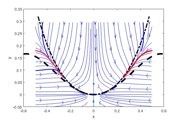
Figure 4. The nullclines $y=x\sin x$ and $y=xT(x)$ of the truncated dynamical system (5) are marked with the dashed lines. Trajectories with initial conditions in the upper half plane are eventually trapped between the two nullclines before converging to the origin. For (5), the origin is an asymptotically stable fixed point, inconsistent with the system (3) that originated the approximation.

We now demonstrate the application of the framework developed in the Appendix of this paper for the approximation of the center manifold function $z=h(x,y)$ and the study of stability for (3). For a given $(x,y)$ we think of the value of $h(x,y)$ as the fixed point function (evaluated at zero) for an operator $\Gamma_{(x,y)}$ defined on a space of slow-growing functions. We approximate $h(x,y)$ by using small deviations from the iterates of the operator $\Gamma_{(x,y)},$ while keeping track of the accumulated errors. For (3) we achieve enough precision in one iterate.

To initiate the approximation for (3), we solve for $z$ in the equation of the nullcline $\dot{z}=0.$ We get that $z=\Psi(x,y)=x(y-x\sin x)(\sin x+x\cos x)+x\sin x.$ A first application of the contraction operator (71) gives

$$\Gamma_{(x,y)}(x,y,\Psi)-\left[\begin{array}[]{c}x\\ y\\ \Psi(x,y)\end{array}\right]=t\left[\begin{array}[]{l}x(y-x\sin x)\\ -y^{2}(y-\Psi(x,y))\\ 0\end{array}\right]=t(y-x\sin x)\mathcal{O}(|x,y|).$$

We conclude that the central manifold map $h(x,y)$ can be expressed as $\Psi(x,y)+(y-x\sin x)\mathcal{O}(|x,y|).$ Since the term $x(y-x\sin x)(\sin x+x\cos x)$ from $\Psi$ is of the order $(y-x\sin x)\mathcal{O}(|x,y|)$, based on our technique we get:

$$h(x,y)=x\sin x+(y-x\sin x)\mathcal{O}(|x,y|)$$

and, therefore, the flow on the central manifold reduces to

$$\begin{array}[]{l}\dot{x}=x(y-x\sin x)\\ \dot{y}=-y^{2}(y-x\sin x)[1+\mathcal{O}(||(x,y)||)]\end{array}$$ (6)

We note that System $(\ref{TaylorexampleReduced})$ faithfully captures the equilibrium points at locations $(x,x\sin x)$ and the behavior of the trajectories as converging to the origin or to an off-origin equilibrium point, depending on whether the initial condition was in $\{(x_{0},y_{0})\;|x_{0}=0\;\mbox{ or }\;y_{0}<x_{0}\sin x_{0}\}$ or not.

2. Preliminaries

In this section we introduce the terminology, which we mainly borrow from [22], and discuss some dynamical properties of (1), including solutions with stationary center of mass, circular solutions, and fixed points.

Observe that the set of solutions of (1) is

• translation invariant,

• rotation invariant,

• invariant with respect to the reflections about the coordinate axes, that is, with respect to the transformations $y\mapsto-y$ and $x\mapsto-x$.

Thus, if $(\mathrm{r}_{1},\dots\mathrm{r}_{n})$ is a solution of the system, then $(e^{i\theta}\mathrm{r}_{1},\dots e^{i\theta}\mathrm{r}_{n})$ and $(\mathrm{r}_{1}+c,\dots\mathrm{r}_{n}+c)$ are also solutions for any $\theta\in\mathbb{R}$ and any $c\in\mathbb{C}$.

The system decouples whenever the center of mass is stationary. For example, this can happen when the set of $n$ particles can be partitioned into subsets with rotational symmetries. We say that the particles $\{k_{1},k_{2},\dots k_{p}\}$ have rotational symmetry about the point $\mathrm{R}_{0}$ if $\displaystyle\mathrm{r}_{k_{m}}(t)-\mathrm{R}_{0}=e^{(m-1)\frac{2\pi}{p}i}(\mathrm{r}_{k_{1}}(t)-\mathrm{R}_{0}),$ for $m=1,\ldots,p,\;t\geq 0.$

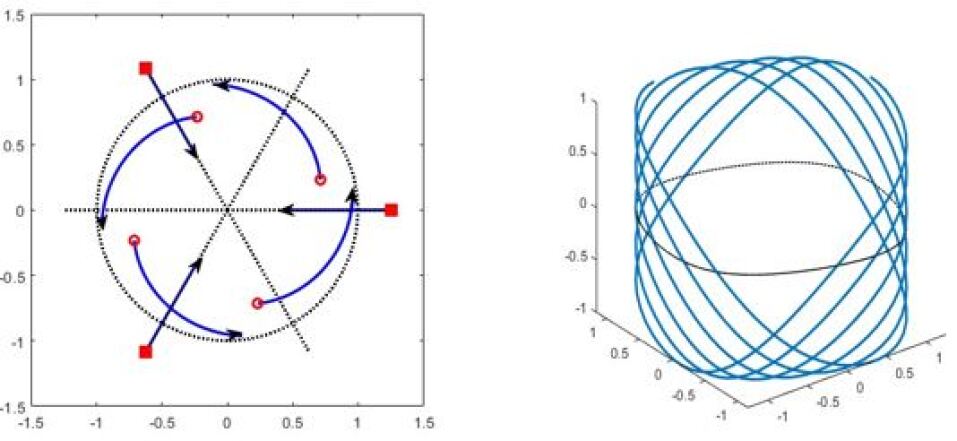
Figure 5. An illustration of a 7-agent/28-dimensional system partitioned into a set of three 1-dimensional Van der Pol oscillators (the square markers) and four rotating agents (the hollow markers), having the center of mass at $(0,0)$ for all times $t$. Left: The positions of the agents from $t=0$ to $t=1.5$ are given by the solid curves, where their limit cycles are represented by the dashed curves. Right: the projection on a 2-dimensional subspace (the dotted line) and on a 3-dimensional subspace (solid line) of $\mathbb{R}^{28}$ of the curve $(x_{1}(t),x_{2}(t),\dots\dot{y}_{7}(t))$ for the oscillators on the left. The subspaces used are $(x_{1},\dot{x}_{1})$ and $(x_{1},\dot{x}_{1},x_{4}).$

Asymptotic decoupling, say, as in Figure 1, is often observed in simulations with random initial conditions and relatively small velocities. However, as with any multidimensional system of oscillators, the limit behavior can be very complex, see Figure 6.

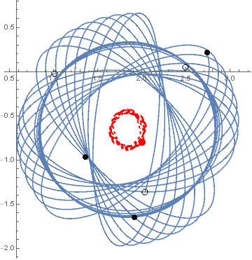
Figure 6. Numerically simulated asymptotic behavior of (1) with $n=3$. The initial conditions are $\bar{r}(0)=[(2.04,-1.36),(2.49,0.05),(1,-0.02)]$, $\dot{\bar{r}}(0)=[(0.34,1.16),(0.77,-0.51),(-0.76,-0.34)]$. The positions of the agents at $t=0$ (at $t=50$) are represented as hollow (solid) dots. The center of mass, represented by the red dot, $R(t)$ moves along a nontrivial cycle (the dashed curve).

Our next goal is to describe the solutions of the system under the assumption that the center of mass is stationary and is centered at the origin. Setting $R=0$ in (1), we obtain

$$\ddot{r}=(1-\dot{r}\cdot\dot{r})\dot{r}-r$$ (7)

Consider a solution $\{r,\dot{r}\}$ of Equation (7). If the vectors $r$ and $\dot{r}$ are parallel at some instant, then they remain parallel and we can describe them as $r(t)=c(t)\hat{r}$ and $\dot{r}(t)=\dot{c}(t)\hat{r}$ for some constant unit vector $\hat{r}$ and a real-valued function $c$ in which case the function $c(t)$ must solve the equation $\ddot{c}=\dot{c}-\dot{c}^{3}-c$. Setting $x=\dot{c}$, $y=-c$, and $f(x)=x^{3}-x$, we obtain the system $\dot{x}=y-f(x)$, $\dot{y}=-x$, which belongs to the class of Liénard systems. The function $f(x)$ satisfies the Liénard theorem [14], see also [15] for a more general discussion, which guarantees the existence of a unique nontrivial limit cycle and this limit cycle is stable. The zero solution of (7) is unstable.

Figure 7. Typical limit behavior of the decoupled system. The trajectory converges to the limit cycle $r(t)=e^{it}$.

The following result shows that the unit circle is the compact global attractor of (7) for all trajectories whose position vectors and the velocity vectors are not initially parallel. Furthermore, we show that as expected by the physical considerations, the direction of the rotation is prescribed by the angle between the vectors $r$ and $\dot{r}$.

Theorem 2.1.

Let $\{r,\dot{r}\}$ be a solution of (7) and $\phi$ be the angle between the vectors $r$ and $\dot{r}$ when measured in the counter-clock wise direction starting from the vector $r$. If $0<\phi<\pi$ ($\pi<\phi<2\pi$) at some instant, then the solution $r$ converges to a limit cycle ${\mathrm{r}}_{+}(t)=e^{i\theta_{*}}e^{it}$ ($\mathrm{r}_{-}(t)=e^{i\theta_{*}}e^{i(-t)}$) for some phase angle $\theta_{*}$. The limit cycles ${\mathrm{r}}_{+}$ and ${\mathrm{r}}_{-}$ are stable.

Proof.

Setting $r=(x,y)$, $u=\dot{x}$, and $v=\dot{y}$, we can rewrite (7) as

$$\begin{split}\dot{x}&=u\\ \dot{y}&=v\\ \dot{u}&=(1-u^{2}-v^{2})u-x\\ \dot{v}&=(1-u^{2}-v^{2})v-y\\ \end{split}$$ (8)

The derivative of the function $vx-uy$ along trajectories of (8) is equal to $\left(1-u^{2}-v^{2}\right)(vx-uy)$. This implies that if at some time instance we have that $vx=uy$, then the vectors $r$ and $\dot{r}$ are parallel (or zero) at all times, and the system reduces to the one-dimensional case. We are therefore interested in the behavior of the system only in the region $vx\neq uy$, which we call $\Omega$:

$$\Omega=\{(u,v,x,y)\in\mathbb{R}^{4}:vx\neq uy\}$$

Note that the subsets $\Omega_{+}$ and $\Omega_{-}$ of $\Omega$ satisfying $vx-uy>0$ and $vx-uy<0$, respectively, are invariant. Define the function $L:\Omega\rightarrow\mathbb{R}$ as follows:

$$L=x^{2}+y^{2}+u^{2}+v^{2}-\log((vx-uy)^{2})$$

Differentiating $L$ along trajectories of (8) yields:

$$\dot{L}=-2(1-u^{2}-v^{2})^{2}\leq 0$$

This indicates that $L$ is decreasing along trajectories of System (8). We may note that

$$\begin{split}L&=x^{2}+y^{2}+u^{2}+v^{2}-\log((vx-uy)^{2})\\ &=x^{2}+y^{2}+u^{2}+v^{2}-\log((x^{2}+y^{2})(u^{2}+v^{2})-(xu+yv)^{2})\\ &\geq x^{2}+y^{2}+u^{2}+v^{2}-\log((x^{2}+y^{2})(u^{2}+v^{2}))\\ &=(x^{2}+y^{2}-\log(x^{2}+y^{2}))+(u^{2}+v^{2}-\log(u^{2}+v^{2}))\end{split}$$

Therefore, as $(x^{2}+y^{2})\rightarrow\infty$ or $(u^{2}+v^{2})\rightarrow\infty$, $L\rightarrow\infty$. This shows that $L$ is radially unbounded. Since, $t-\log(t)\geq 1$ for all $t>0$, we obtain that $L\geq 2$. In fact, the minimum value of $L$ is 2. The function $L$ attains its minimum value on the set $\Omega_{\min}=\{(u,v,x,y)\in\Omega:(u^{2}+v^{2}=1),(x^{2}+y^{2}=1),(vx-uy=\pm 1)\}$.

Thus, according to Lasalle’s Invariance Principle, every trajectory approaches the largest invariant set inside $\Omega_{\min}$. The trajectories contained entirely in $\Omega_{\min}$ correspond to the solutions of the form $ce^{it}$ and $ce^{-it}$, $c\in\mathbb{C}$, $|c|=1$.

Thus, if $0<\phi<\pi$, then the $(x,y,u,v)$-representation of the solution $\{r,\dot{r}\}$ lies inside $\Omega_{+}$ and this solution will have $\mathrm{r}_{+}$ as its limit cycle. Similarly, the solutions for which $\pi<\phi<2\pi$ will approach a limit cycle $\mathrm{r}_{-}$. ∎

Definition 2.2.

(1) A rotating state is any solution of (1) such that the center of mass of the system is stationary and the particles rotate in the same direction about the stationary center of mass with a unit angular velocity. In another words, a rotating state is any solution of the form $\mathrm{r}_{k}(t)=e^{it}e^{i\theta_{k}}+c$, for all $k=1,\dots n$ or $\mathrm{r}_{k}(t)=e^{-it}e^{i\theta_{k}}+c$, for all $k=1,\dots n,$ where $c\in\mathbb{C}$ is a constant vector, and the polar angles $\{\theta_{k}\}$ satisfy: $\sum_{k=1}^{n}e^{i\theta_{k}}=0$.

(2) We call a rotating state degenerate if there is $\theta_{*}\in[0,2\pi)$ and $\phi_{j}\in\{0,\pi\}$ such that $\theta_{j}=\theta_{*}+\phi_{j}$, that is, the particles split into two equinumerous polar-opposite groups that rotate about the stationary center of mass with a unit angular velocity. Degenerate rotating states can arise only for an even number of particles.

Following Theorem 2.1, if the center of mass is stationary, the limit states of the decoupled system are precisely the rotating states.

3. Change of Coordinates about $\mathrm{r}_{k}=e^{it}e^{i\theta_{0k}}$

In the following three sections we prove the main result of the paper. Since the system is translation and reflection invariant, it suffices to establish our main result for rotating states about the origin with all agents spinning counterclockwise. In the present section, we introduce a change of coordinates in which the original rotating states centered at the origin form fixed points. We also calculate the Jacobian of the new system, see Equation (15).

We perform the change of coordinates in two steps: we first introduce the auxiliary coordinate system $\{X_{k},Y_{k}\}$ by setting $\mathrm{r}_{k}=e^{it}(X_{k}+iY_{k})$, which we refer to as the rotating frame, then we perform rotations (that depend on the parameters $\theta_{0k}$) and translations within the $(X_{k},Y_{k})$ and $(\dot{X}_{k},\dot{Y}_{k})$ coordinate planes to have the fixed points of interest located at the origin.

In Equation (1), switching to new coordinates $X_{k}$ and $Y_{k}$ by the substitution $\mathrm{r}_{k}=e^{it}(X_{k}+iY_{k})$, we obtain the system of equations

$$\begin{split}\ddot{X}_{k}&=2\dot{Y}_{k}+\left(1-(\dot{X}_{k}-Y_{k})^{2}-(X_{k}+\dot{Y}_{k})^{2}\right)(\dot{X}_{k}-Y_{k})+\bar{X}\\ \ddot{Y}_{k}&=-2\dot{X}_{k}+\left(1-(\dot{X}_{k}-Y_{k})^{2}-(X_{k}+\dot{Y}_{k})^{2}\right)(X_{k}+\dot{Y}_{k})+\bar{Y}\end{split}$$ (9)

where $\bar{X}=(X_{1}+\cdots+X_{n})/n$ and $\bar{Y}=(Y_{1}+\cdots+Y_{n})/n$. Our next results describes the set of equilibrium points for (9).

Lemma 3.1.

A point $(X_{0k},Y_{0k},\dot{X}_{0k},\dot{Y}_{0k})$, $k=1,\ldots,n$, is an equilibrium point of (9) if and only if (i) $\dot{X}_{0k}=0$, $\dot{Y}_{0k}=0$ for all $k$, (ii) $\bar{X}_{0}=\bar{Y}_{0}=0$ and (iii) for all $k$, either $X_{0k}=Y_{0k}=0$ or $X_{0k}=\cos(\delta_{k})$, $Y_{0k}=\sin(\delta_{k})$ for some constants $\delta_{k}$.

Note that the fixed points of (9), seen in the original coordinates, correspond to having a juxtaposition between $p$ particles placed at the origin (an unstable fixed point) and $N-p$ particles in a rotating state about the origin.

Proof.

For convenience, we are dropping the zero subscripts. Equating the right-hand sides of (9) to zero, setting $\dot{X}_{k}=0$ and $\dot{Y}_{k}=0$, and solving for $\bar{X}$ and $\bar{Y}$, we obtain that for all $k$

$$\bar{X}=-(1-X_{k}^{2}-Y_{k}^{2})Y_{k}\mbox{ and }\bar{Y}=(1-X_{k}^{2}-Y_{k}^{2})X_{k}.$$ (10)

It follows that

$$(\bar{X})^{2}+(\bar{Y})^{2}=(1-(X_{k}^{2}+Y_{k}^{2}))^{2}(X_{k}^{2}+Y_{k}^{2}),\quad k=1,\ldots,n.$$ (11)

Set $s=(\bar{X})^{2}+(\bar{Y})^{2}$. We claim that $s=0$. Indeed, assume towards contradiction that $s>0$. Consider the function $f(t)=(1-t)^{2}t$ for $t\geq 0$. Then each value $s_{k}=X_{k}^{2}+Y_{k}^{2}$ is a solution of the equation $f(s_{k})=s$. Note that $s_{k}\neq 1$ for otherwise $s=f(s_{k})=0$. Solving (10) for $X_{k}$ and $Y_{k}$, we get that

$$X_{k}=\frac{\bar{Y}}{(1-s_{k})^{2}}\mbox{ and }Y_{k}=-\frac{\bar{X}}{(1-s_{k})^{2}}.$$

It follows that

$$\bar{X}=\frac{1}{n}\sum_{k}\frac{\bar{Y}}{(1-s_{k})^{2}}\mbox{ and }\bar{Y}=-\frac{1}{n}\sum_{k}\frac{\bar{X}}{(1-s_{k})^{2}}.$$

Multiplying both sides of the first equation by $\bar{X}$ and the second equation by $\bar{Y}$ and then adding them together, we obtain that $s=(\bar{X})^{2}+(\bar{Y})^{2}=0$, which is a contradiction.

Thus $s=0$. It follows from Equation (11) that either $(X_{k},Y_{k})=0$ or $X_{k}^{2}+Y_{k}^{2}=1$. Denote by $I$ the set of indices $k$ such that $X_{k}^{2}+Y_{k}^{2}=1$. For $k\in I$, choose $\delta_{k}\in[0,2\pi]$ such that $(X_{k},Y_{k})=(\cos(\delta_{k}),\sin(\delta_{k})).$ Note that $\sum_{k\in I}e^{i\delta_{k}}=n(\bar{X}+i\bar{Y})=0$. Conversely, we notice that any family $(X_{k},Y_{k})$ of constant functions such that $X_{k}=Y_{k}=0$ or $X_{k}=\cos(\delta_{k})$, $Y_{k}=\sin(\delta_{k})$ with $\bar{X}=\bar{Y}=0$ is an equilibrium solution for (9). The result now follows.

∎

The rotating states about the origin of (1) correspond to the fixed points of (9) that are within the set $\displaystyle\bigcap_{k=1}^{n}\{X_{k}^{2}+Y_{k}^{2}=1\}$. We denote this subset of fixed points by $\mathcal{F}$. The $\epsilon$-$\delta$ formulation of Theorem (1.1) when $R_{0}=0$ is equivalent to the classical stability and limit cycle asymptotic result for the fixed points of (9) in $\mathcal{F}.$

The second step of the coordinate change is dependent on the parameters of the rotating state; it uses translations and rotations so that the analysis becomes centered about the origin.

Fix a rotating state $\mathrm{r}_{k}=e^{it}e^{i\theta_{0k}}$. Notice that $\sum_{k=1}^{n}e^{i\theta_{0k}}=0$. Shifting the phases by the same angle $\theta^{*}$ gives a new rotating state $\mathrm{r}_{k}=e^{it}e^{i(\theta_{0k}+\theta^{*})}$ with the same stability characteristics.

Notice also that we can always find $\theta^{*}$ such that $\displaystyle\sum_{k}\sin(\theta_{0k}+\theta^{*})\cos(\theta_{0k}+\theta^{*})=0$ since

$$\sum_{k}\sin(\theta_{0k}+\theta^{*})\cos(\theta_{0k}+\theta^{*})\\ =\left(\frac{1}{2}\sum_{k}\sin(2\theta_{0k})\right)\cos(2\theta^{*})+\left(\frac{1}{2}\sum_{k}\cos(2\theta_{0k})\right)\sin(2\theta^{*})$$

and for any choice of real numbers $A$ and $B$, the equation $A\sin(2\theta^{*})+B\cos(2\theta^{*})=0$ always has a solution $\theta^{*}$.

Thus, working with phase-shifted rotating states if necessary, we can additionally assume that the polar angles $\{\theta_{0k}\}$ of the rotating state satisfy:

$$\sum_{k=1}^{n}\cos(\theta_{0k})\sin(\theta_{0k})=0.$$ (12)

Definition 3.2.

Consider the following change of coordinates

$$\mathrm{r}_{k}(t)=e^{it}e^{i\theta_{0k}}\big{[}(a_{k}(t)+1)+ib_{k}(t)\big{]},\mbox{ where }a_{k},b_{k}\in\mathbb{R}.$$ (13)

Let $u_{k}=\dot{a}_{k}$ and $w_{k}=\dot{b}_{k}.$

The starting rotating state solution $\mathrm{r}_{k}=e^{it}e^{i\theta_{0k}}$, $\dot{\mathrm{r}}_{k}=ie^{it}e^{i\theta_{0k}}$, $k=1,\ldots,n$, corresponds to the fixed point $a_{k}=0$, $b_{k}=0$, $u_{k}=0$, $w_{k}=0$, $k=1,\ldots,n$, in the new coordinates.

We notice that the rotating frame coordinates $\{X_{k},Y_{k}\}$ relate to $\{a_{k},b_{k}\}$ as

$$(X_{k}+iY_{k})=e^{i\theta_{0k}}(a_{k}+1+ib_{k}),$$

via an affine transformation. We get

$$\begin{split}\dot{\mathrm{r}}_{k}&=e^{it}e^{i\theta_{0k}}\big{[}(\dot{a}_{k}-b_{k})+i((a_{k}+1)+\dot{b}_{k})\big{]}\\ \ddot{\mathrm{r}}_{k}&=e^{it}e^{i\theta_{0k}}\big{[}(\ddot{a}_{k}-2\dot{b}_{k}-a_{k}-1)+i(\ddot{b}_{k}+2\dot{a}_{k}-b_{k})\big{]}.\end{split}$$ (14)

Note that

$$1-|\dot{\mathrm{r}}_{k}|^{2}=1-(\dot{a}_{k}-b_{k})^{2}-(a_{k}+1+\dot{b}_{k})^{2}=-(\dot{a}_{k}-b_{k})^{2}-2(a_{k}+\dot{b}_{k})-(a_{k}+\dot{b}_{k})^{2}.$$

Thus, substituting Equations (14) into System (1) and dividing both sides by $e^{it}e^{i\theta_{0k}}$, we get

$$(\ddot{a}_{k}-2\dot{b}_{k}-a_{k}-1)+i(\ddot{b}_{k}+2\dot{a}_{k}-b_{k})\\ =\big{[}1-(\dot{a}_{k}-b_{k})^{2}-((a_{k}+1)+\dot{b}_{k})^{2}\big{]}\big{(}\dot{a}_{k}-b_{k})+i((a_{k}+1)+\dot{b}_{k}\big{)}\\ -(a_{k}+1+ib_{k})+\frac{1}{n}\sum_{m=1}^{n}e^{i(\theta_{0m}-\theta_{0k})}(a_{m}+1+ib_{m}).$$

Note that $\sum_{m=1}^{n}e^{i(\theta_{0m}-\theta_{0k})}=0$. Now separating the real part and imaginary part and using $u_{k}=\dot{a}_{k}$ and $w_{k}=\dot{b}_{k}$, we obtain the system

$$\begin{split}\dot{a}_{k}&=u_{k}\\ \dot{b}_{k}&=w_{k}\\ \dot{u}_{k}&=\begin{multlined}2w_{k}-\big{[}(u_{k}-b_{k})^{2}+2(a_{k}+w_{k})+(a_{k}+w_{k})^{2}\big{]}(u_{k}-b_{k})\\ +\frac{1}{n}\sum_{m=1}^{n}\cos(\theta_{0m}-\theta_{0k})a_{m}-\frac{1}{n}\sum_{m=1}^{n}\sin(\theta_{0m}-\theta_{0k})b_{m}\end{multlined}2w_{k}-\big{[}(u_{k}-b_{k})^{2}+2(a_{k}+w_{k})+(a_{k}+w_{k})^{2}\big{]}(u_{k}-b_{k})\\ +\frac{1}{n}\sum_{m=1}^{n}\cos(\theta_{0m}-\theta_{0k})a_{m}-\frac{1}{n}\sum_{m=1}^{n}\sin(\theta_{0m}-\theta_{0k})b_{m}\\ \dot{w}_{k}&=\begin{multlined}-2u_{k}-2a_{k}-2w_{k}-\big{[}(u_{k}-b_{k})^{2}+(a_{k}+w_{k})^{2}\big{]}\\ -\big{[}(u_{k}-b_{k})^{2}+2(a_{k}+w_{k})+(a_{k}+w_{k})^{2}\big{]}(a_{k}+w_{k})\\ +\frac{1}{n}\sum_{m=1}^{n}\sin(\theta_{0m}-\theta_{0k})a_{m}+\frac{1}{n}\sum_{m=1}^{n}\cos(\theta_{0m}-\theta_{0k})b_{m}\end{multlined}-2u_{k}-2a_{k}-2w_{k}-\big{[}(u_{k}-b_{k})^{2}+(a_{k}+w_{k})^{2}\big{]}\\ -\big{[}(u_{k}-b_{k})^{2}+2(a_{k}+w_{k})+(a_{k}+w_{k})^{2}\big{]}(a_{k}+w_{k})\\ +\frac{1}{n}\sum_{m=1}^{n}\sin(\theta_{0m}-\theta_{0k})a_{m}+\frac{1}{n}\sum_{m=1}^{n}\cos(\theta_{0m}-\theta_{0k})b_{m}\end{split}$$ (15)

Because the rotating frame coordinates $\{X_{k},Y_{k}\}$ relates to $\{a_{k},b_{k}\}$ via an affine transformation, there is a one-to-one correspondence between equilibrium points of these systems. Lemma 3.1 gives a full description of equilibrium points for the rotating frame. Thus, each point of the form $(X_{0k}=\cos(\delta_{k}^{\prime}),Y_{0k}=\sin(\delta_{k}^{\prime}),\dot{X}_{0k}=0,\dot{Y}_{0k}=0)$, corresponds to the fixed point $(a_{k}=-1+\cos(\delta_{k}^{\prime}-\theta_{0k}),b_{k}=\sin(\delta_{k}^{\prime}-\theta_{0k}),u_{k}=0,w_{k}=0)$. Thus, renaming $\delta_{k}^{\prime}-\theta_{0k}$ as $\delta_{k}$, we obtain a complete description of the set of equilibrium points in the $\{a,b,u,w\}$-coordinates.

Lemma 3.3.

Let

$$\Delta=\{(\delta_{1},\ldots,\delta_{n})\in\mathbb{R}^{n}:\sum_{k=1}^{n}e^{i(\theta_{0k}+\delta_{k})}=0\},$$

and let $\mathcal{R}\subset\mathbb{R}^{4n}$ denote

$$\mathcal{R}=\left\{a_{k}=cos(\delta_{k})-1,b_{k}=\sin(\delta_{k}),u_{k}=0,w_{k}=0:\{\delta_{k}\}\in\Delta\right\}.$$

Then $\mathcal{R}$ consists of all equilibrium solutions of (15) near the origin.

Remark 3.4.

(1) It is helpful to think of the set $\Delta$ in the lemma above as the set of parameters encoding all possible perturbations of the rotating state $(\theta_{01},\ldots,\theta_{0n})$ within the family of rotating states about the origin. The set $\Delta$ can also be seen as the set of parameters encoding the fixed points of System (15) near the origin.

(2) Set

$$f_{1}(\delta_{1},\ldots,\delta_{n})=\sum_{k=1}^{n}\left(\cos\theta_{0k}\cos\delta_{k}-\sin\theta_{0k}\sin\delta_{k}\right)$$

and

$$f_{2}(\delta_{1},\ldots,\delta_{n})=\sum_{k=1}^{n}\left(\cos\theta_{0k}\sin\delta_{k}+\sin\theta_{0k}\cos\delta_{k}\right).$$

The set $\Delta$ was defined as the set of all solutions to the system of two equations, $f_{1}(\delta_{1},\dots\delta_{n})=0$ and $f_{2}(\delta_{1},\dots\delta_{n})=0$. Thus, barring any degeneracies at the origin, $\Delta$ should have the local structure of an $(n-2)$-dimensional manifold. Note that for the map $(f_{1},f_{2})$ from $\mathbb{R}^{n}$ to $\mathbb{R}^{2}$ the linearization at the origin (derivatives taken with respect to $\delta_{1},\ldots,\delta_{n}$) is the matrix with columns $-(\sin(\theta_{01}),\ldots,\sin(\theta_{0n}))^{T}$ and $(\cos(\theta_{01}),\ldots,\cos(\theta_{0n}))^{T}.$

Definition 3.5.

For a rotating state $\mathrm{r}_{k}=e^{it}e^{i\theta_{0k}}$ satisfying (12) denote by $\bar{c}$ and $\bar{s}$ the column-vectors

$$\bar{c}=(\cos(\theta_{01}),\ldots,\cos(\theta_{0n}))^{T}\mbox{ and }\bar{s}=(\sin(\theta_{01}),\ldots,\sin(\theta_{0n}))^{T}.$$

Note that equation (12) ensures that the vectors $\bar{c}$ and $\bar{s}$ are orthogonal in $\mathbb{R}^{n}.$ Unless one of them is the zero vector, $\bar{c}$ and $\bar{s}$ span a two-dimensional linear space. The equality $\bar{c}=0$ implies that $\sin\theta_{0k}=\pm 1,$ and given that $\sum_{k=1}^{n}e^{i\theta_{0k}}=0,$ that can only be satisfied if $n$ is even, with half of the angles $\theta_{0k}$ equal to $\pi/2$ and the other half equal to $-\pi/2.$ The equation $\bar{s}=0$ can only be satisfied if $n$ is even, with half of the angles $\theta_{0k}$ equal to $0$ and the other half equal to $\pi.$ Either way, the span of $\bar{c}$ and $\bar{s}$ is two dimensional except for the degenerate rotating states.

Returning to the sets $\Delta$ and $\mathcal{R}$ from Lemma 3.3: if the angles $\theta_{0k}$ are not from a degenerate configuration, then the map $(f_{1},f_{2})$ used to implicitly define $\Delta$ has full rank at the origin, therefore near the origin of $\mathbb{R}^{n}$ the set $\Delta$ is an $n-2$ manifold. Similarly, the set $\mathcal{R}$ of fixed points for (15) is also an $(n-2)$-dimensional manifold near the origin in $\mathbb{R}^{4n}$.

Jacobian. We finish this section by calculating the Jacobian $J$ of (15) about the origin. The rows and the columns of the Jacobian are indexed by the variables $\{\{a_{k}\},\{b_{k}\},\{u_{k}\},\{w_{k}\}\}$ and their derivatives, respectively. Then

$$J=\hbox{}\vbox{\kern 0.86108pt\hbox{$\kern 0.0pt\kern 2.5pt\kern-5.0pt\left(\kern 0.0pt\kern-2.5pt\kern-6.66669pt\vbox{\kern-0.86108pt\vbox{\vbox{ \halign{\kern\arraycolsep\hfil\@arstrut$\kbcolstyle#$\hfil\kern\arraycolsep& \kern\arraycolsep\hfil$\@kbrowstyle#$\ifkbalignright\relax\else\hfil\fi\kern\arraycolsep&& \kern\arraycolsep\hfil$\@kbrowstyle#$\ifkbalignright\relax\else\hfil\fi\kern\arraycolsep\cr 5.0pt\hfil\@arstrut$\scriptstyle$\hfil\kern 5.0pt&5.0pt\hfil$\scriptstyle\partial a$\hfil\kern 5.0pt&5.0pt\hfil$\scriptstyle\partial b$\hfil\kern 5.0pt&5.0pt\hfil$\scriptstyle\partial u$\hfil\kern 5.0pt&5.0pt\hfil$\scriptstyle\partial w\\\partial\dot{a}$\hfil\kern 5.0pt&5.0pt\hfil$\scriptstyle\textrm{O}_{n}$\hfil\kern 5.0pt&5.0pt\hfil$\scriptstyle\textrm{O}_{n}$\hfil\kern 5.0pt&5.0pt\hfil$\scriptstyle\textrm{I}_{n}$\hfil\kern 5.0pt&5.0pt\hfil$\scriptstyle\textrm{O}_{n}\\\partial\dot{b}$\hfil\kern 5.0pt&5.0pt\hfil$\scriptstyle\textrm{O}_{n}$\hfil\kern 5.0pt&5.0pt\hfil$\scriptstyle\textrm{O}_{n}$\hfil\kern 5.0pt&5.0pt\hfil$\scriptstyle\textrm{O}_{n}$\hfil\kern 5.0pt&5.0pt\hfil$\scriptstyle\textrm{I}_{n}\\\partial\dot{u}$\hfil\kern 5.0pt&5.0pt\hfil$\scriptstyle C$\hfil\kern 5.0pt&5.0pt\hfil$\scriptstyle-S$\hfil\kern 5.0pt&5.0pt\hfil$\scriptstyle\textrm{O}_{n}$\hfil\kern 5.0pt&5.0pt\hfil$\scriptstyle 2\textrm{I}_{n}\\\partial\dot{w}$\hfil\kern 5.0pt&5.0pt\hfil$\scriptstyle S-2\textrm{I}$\hfil\kern 5.0pt&5.0pt\hfil$\scriptstyle C$\hfil\kern 5.0pt&5.0pt\hfil$\scriptstyle-2\textrm{I}_{n}$\hfil\kern 5.0pt&5.0pt\hfil$\scriptstyle-2\textrm{I}_{n}$\hfil\kern 5.0pt\crcr}}}}\right)$}}$$ (16)

where $\textrm{O}_{n}$ is the $n\times n$ zero matrix, $\textrm{I}_{n}$ is the $n\times n$ identity matrix,

$$S=\left\{\frac{1}{n}\sin(\theta_{0m}-\theta_{0k})\right\}_{k,m=1}^{n}\mbox{ and }C=\left\{\frac{1}{n}\cos(\theta_{0m}-\theta_{0k})\right\}_{k,m=1}^{n}.$$

4. Stability of Non-Degenerate Rotating States

In this section, we introduce a basis for $\mathbb{R}^{4n}$ that allows us to block diagonalize the Jacobian (16) according to the stable and central linear subspaces and we will show that there are no unstable directions. The stability result will then follow from our analysis of the central manifold alone. We note that the matrix $S$ defined above is the zero matrix precisely when the angles $\theta_{0k}$ form a degenerate configuration, which will necessitate a separate treatment of degenerate configurations, see Section 5 for details.

Assume that the rotating state $\mathrm{r}_{k}=e^{it}e^{i\theta_{0k}}$ is non-degenerate. Recall that for non-degenerate rotating states the vectors $\bar{c}$ and $\bar{s}$ span a two-dimensional linear space. We claim that $\mathrm{ker}(S)=\mathrm{ker}(C)=\{\bar{c},\bar{s}\}^{\perp}$, the set of vectors $x\in\mathbb{R}^{n}$ such that $\bar{c}\cdot x=0$ and $\bar{s}\cdot x=0$. Indeed, the $k$-th row of the vector $nSx$ is

$$\begin{split}\sum_{m=1}^{n}\sin(\theta_{0m}-\theta_{0k})x_{m}&=\cos(\theta_{0k})\sum_{m}\sin(\theta_{0m})x_{m}-\sin(\theta_{0k})\sum_{m}\cos(\theta_{0m})x_{m}\\ &=\cos(\theta_{0k})(\bar{s}\cdot x)-\sin(\theta_{0k})(\bar{c}\cdot x).\end{split}$$

Since the vectors $\bar{c}$ and $\bar{s}$ are linearly independent, we obtain that $x\in\mathrm{ker}(S)$ if and only if $x$ is orthogonal to both $\bar{c}$ and $\bar{s}$. Similarly, we can show that $\mathrm{ker}(C)=\{\bar{s},\bar{c}\}^{\perp}$. It follows that $\mathrm{ker}(S)=\mathrm{ker}(C)$ and that the common kernel is a $(n-2)$-dimensional subspace in $\mathbb{R}^{n}$.

Let $\mathbb{V}$ be a matrix whose columns form an orthonormal basis for $\mathrm{ker}(C)=\mathrm{ker}(S)$. Note that the matrix $\mathbb{V}$ is $n\times(n-2)$ dimensional. Consider the linear subspaces $L_{1}$ and $L_{2}$ of $\mathbb{R}^{4n}$ spanned by the columns of the matrices $B_{1}$ and $B_{2}$, respectively, where

$$B_{1}=\left[\begin{array}[]{cccc}\mathbb{V}&\textrm{O}_{n,n-2}&\textrm{O}_{n,n-2}&\textrm{O}_{n,n-2}\\ \textrm{O}_{n,n-2}&\mathbb{V}&\textrm{O}_{n,n-2}&\textrm{O}_{n,n-2}\\ \textrm{O}_{n,n-2}&\textrm{O}_{n,n-2}&\mathbb{V}&\textrm{O}_{n,n-2}\\ \textrm{O}_{n,n-2}&\textrm{O}_{n,n-2}&\textrm{O}_{n,n-2}&\mathbb{V}\\ \end{array}\right],\;B_{2}=\left[\begin{array}[]{cccccccc}\bar{c}&\bar{s}&0&0&0&0&0&0\\ 0&0&\bar{c}&\bar{s}&0&0&0&0\\ 0&0&0&0&\bar{c}&\bar{s}&0&0\\ 0&0&0&0&0&0&\bar{c}&\bar{s}\\ \end{array}\right]$$

Here $\textrm{O}_{n,n-2}$ is the $n\times(n-2)$-zero matrix. Note that $\mathbb{R}^{4n}=L_{1}\oplus L_{2}$, $L_{1}\perp L_{2}$, $\mathrm{dim}(L_{1})=4n-8$, and $\mathrm{dim}(L_{2})=8$.

We show next that in the basis given by $[B_{1}\;B_{2}]$ the Jacobian $J$ has a block-diagonal form, with blocks $J_{1}$ and $J_{2}$ of dimensions $(4n-8)\times(4n-8)$ and $8\times 8$ respectively, where $J_{1}$ is given in (19) and $J_{2}$ is given in (20).

We need to show that $J[B_{1}\;B_{2}]=[B_{1}\;B_{2}]\mbox{diag}\{J_{1},J_{2}\},$ i.e. that $JB_{1}=B_{1}J_{1}$ and $JB_{2}=B_{2}J_{2}.$

From (16) we get:

$$JB_{1}=\left[\begin{array}[]{cccc}\textrm{O}_{n,n-2}&\textrm{O}_{n,n-2}&\mathbb{V}&\textrm{O}_{n,n-2}\\ \textrm{O}_{n,n-2}&\textrm{O}_{n,n-2}&\textrm{O}_{n,n-2}&\mathbb{V}\\ \textrm{O}_{n,n-2}&\textrm{O}_{n,n-2}&\textrm{O}_{n,n-2}&2\mathbb{V}\\ -2\mathbb{V}&\textrm{O}_{n,n-2}&-2\mathbb{V}&-2\mathbb{V}\\ \end{array}\right]$$ (17)

Set $f=\frac{1}{n}\sum_{k=1}^{n}\cos^{2}(\theta_{k})$ and $d=\frac{1}{n}\sum_{k=1}^{n}\sin^{2}(\theta_{k})$. Then, using Equation (12), one can check that

$$\begin{split}C\bar{c}=f\bar{c},&\qquad S\bar{c}=-f\bar{s},\\ C\bar{s}=d\bar{s},&\qquad S\bar{s}=d\bar{c}.\end{split}$$

It follows that

$$JB_{2}=\left[\begin{array}[]{cccccccc}\bar{0}&0&0&0&\bar{c}&\bar{s}&0&0\\ 0&0&0&0&0&0&\bar{c}&\bar{s}\\ f\bar{c}&d\bar{s}&f\bar{s}&-d\bar{c}&0&0&2\bar{c}&2\bar{s}\\ -2\bar{c}-f\bar{s}&d\bar{c}-2\bar{s}&f\bar{c}&d\bar{s}&-2\bar{c}&-2\bar{s}&-2\bar{c}&-2\bar{s}\\ \end{array}\right].$$ (18)

Note that $L_{1}$ and $L_{2}$ are $J$-invariant subspaces. Thus, to describe the spectrum of the Jacobian it is enough to do so for the restrictions $J|L_{1}$ and $J|L_{2}$.

Restriction of $J$ onto $L_{1}$. It follows from Equation (17) that the matrix of the restriction of $J$ onto $L_{1}$ in the basis $B_{1}$ has the form

$$J_{1}=\left[\begin{array}[]{cccc}\textrm{O}_{n-2}&\textrm{O}_{n-2}&\textrm{I}_{n-2}&\textrm{O}_{n-2}\\ \textrm{O}_{n-2}&\textrm{O}_{n-2}&\textrm{O}_{n-2}&\textrm{I}_{n-2}\\ \textrm{O}_{n-2}&\textrm{O}_{n-2}&\textrm{O}_{n-2}&2\textrm{I}_{n-2}\\ -2\textrm{I}_{n-2}&\textrm{O}_{n-2}&-2\textrm{I}_{n-2}&-2\textrm{I}_{n-2}\\ \end{array}\right]$$ (19)

Here $\textrm{O}_{n-2}$ is the $(n-2)\times(n-2)$ zero matrix and $I_{n-2}$ is the identity matrix of the same dimension. Using the formula for the determinant for block matrices, we compute the characteristic polynomial

$$\det(J_{1}-\lambda\textrm{I})=\lambda^{n-2}(\lambda^{3}+2\lambda^{2}+4\lambda+4)^{n-2}.$$

The eigenvalues of $J_{1}$ are $\lambda=0$, $\lambda\approx-0.35+1.72i$, $\lambda\approx-0.35-1.72i$, $\lambda\approx-1.29$, each of geometric multiplicity $n-2$.

Restriction of $J$ onto $L_{2}$. Observe that $d+f=1$. Set $\omega$ such that $f=1/2+\omega$ and $d=1/2-\omega$. Then using Formula (18), we find the matrix of the restriction of $J$ onto $L_{2}$ in the basis $B_{2}$:

$$\begin{split}J_{2}&=\left(\begin{array}[]{c|c}\textrm{O}_{4}&\textrm{I}_{4}\\ \hline\cr\begin{array}[]{cccc}f&0&0&-d\\ 0&d&f&0\\ -2&d&f&0\\ -f&-2&0&d\\ \end{array}&\begin{array}[]{cccc}0&0&2&0\\ 0&0&0&2\\ -2&0&-2&0\\ 0&-2&0&-2\end{array}\end{array}\right)\\ &=\left(\begin{array}[]{c|c}\textrm{O}_{4}&\textrm{I}_{4}\\ \hline\cr\begin{array}[]{cccc}1/2+\omega&0&0&-1/2+\omega\\ 0&1/2-\omega&1/2+\omega&0\\ -2&1/2-\omega&1/2+\omega&0\\ -1/2-\omega&-2&0&1/2-\omega\\ \end{array}&\begin{array}[]{cccc}0&0&2&0\\ 0&0&0&2\\ -2&0&-2&0\\ 0&-2&0&-2\end{array}\end{array}\right)\end{split}$$ (20)

Then the characteristic polynomial of $J_{2}$ is equal to

$$\det(J_{2}-\lambda I)=(1+\lambda^{2})(1-4\omega^{2}+4\lambda+12\lambda^{2}+14\lambda^{3}+9\lambda^{4}+4\lambda^{5}+\lambda^{6}).$$

Therefore, the spectrum of $J_{2}$ consists of $\pm i$ and zeros of the polynomial $f_{\omega}(\lambda)=1-4\omega^{2}+4\lambda+12\lambda^{2}+14\lambda^{3}+9\lambda^{4}+4\lambda^{5}+\lambda^{6}$. Consider the Hurwitz matrix $H$ for the polynomial $f_{\omega}(\lambda)$:

$$H=\left(\begin{array}[]{cccccc}4&14&4&0&0&0\\ 1&9&12&1-4\omega^{2}&0&0\\ 0&4&14&4&0&0\\ 0&1&9&12&1-4\omega^{2}&0\\ 0&0&4&14&4&0\\ 0&0&1&9&12&1-4\omega^{2}\\ \end{array}\right).$$

The leading principal minors of $H$ are $\Delta_{1}=4$, $\Delta_{2}=22$, $\Delta_{3}=132$, $\Delta_{4}=-352(\omega^{2}-3)$, $\Delta_{5}=-8(-333-636\omega^{2}+128\omega^{4})$, and $\Delta_{6}=8(-1+2\omega)(1+2\omega)(-333-636\omega^{2}+128\omega^{4})$. Note that $-1/2\leq\omega\leq 1/2$, but $\omega=\pm 1/2$ can only hold if $\cos^{2}\theta_{k}=1$ for all $k,$ or if $\sin^{2}\theta_{k}=1$ for all $k,$ which are impossible in a non-degenerate configuration, therefore $-1/2<\omega<1/2$. It is straightforward to check that the leading principal minors of $H$ are strictly positive. By the Routh-Hurwitz criterion [7, Ch. XV, Section 6], the roots of the polynomial $f(\lambda)$ are in the negative half-plane.

Moreover, for $\omega=\pm 1/2$ the polynomial $f_{\pm 1/2}$ has $\lambda=0$ as a simple root, with the remaining five bounded away from the imaginary line (in fact $f_{\pm 1/2}=\lambda(\lambda+1)^{2}(\lambda^{3}+2\lambda^{2}+4\lambda+4)$, consistent with the characteristic polynomial in the next section).

It is interesting to notice that the spectral gap of the Jacobian (16), seen as a function of the angles $\theta_{k,0}$, decreases to zero when the configurations $\{\theta_{k,0}\}_{k=1}^{n}$ approach a degenerate rotating state (only possible if $n$ is even).

Center manifold. We have established that the spectrum of $J$ consists of $n-2$ zero eigenvalues, $i$, $-i$, and $3n$ eigenvalues in the negative half-plane. In particular, we obtained the center manifold of the system is $n$-dimensional.

Note that the presence of the $\pm i$ eigenvalue suggests that the center manifold might contain a one-parameter family of periodic orbits. However, (the presence of) the resonance between the $0$ and $\pm i$ eigenvalues does not allow us to make such a conclusion. Nonetheless, we produce an explicit parametrization of the center manifold and completely describe its structure. In what follows, we show that the rotating states form a center manifold of the system and correspond to periodic solutions in the $\{a,b,u,w\}$-frame, with the magnitude of the translation $R_{0}$ measured off the origin in the original $(x,y,\dot{x},\dot{y})$-coordinates acting as the parameter of the nested family of periodic orbits.

Consider a rotating state $\mathrm{r}_{k}(t)=R_{0}+e^{i(\theta_{0k}+\delta_{k})}e^{it}$, $k=1,\ldots,n$, $R_{0}=|R_{0}|e^{i\rho}$, viewed as a perturbation of the fixed rotating state $\{e^{i\theta_{0k}}e^{it}\}$. Using $(a_{k}+1)+ib_{k}=\mathrm{r}_{k}\;e^{-it}e^{-i\theta_{0k}}$, per Equation (13), and $u_{k},=\dot{a}_{k},\;w_{k}=\dot{b}_{k}$ we can rewrite $\mathrm{r}_{k}$ in the $\{a,b,u,w\}$-coordinates as

$$\left[\begin{array}[]{c}a_{k}\\ b_{k}\\ u_{k}\\ w_{k}\\ \end{array}\right]=\left[\begin{array}[]{c}\cos(\delta_{k})-1\\ \sin(\delta_{k})\\ 0\\ 0\\ \end{array}\right]\\ +|R_{0}|\cos(\rho-t)\left[\begin{array}[]{c}\cos(\theta_{0k})\\ -\sin(\theta_{0k})\\ -\sin(\theta_{0k})\\ -\cos(\theta_{0k})\\ \end{array}\right]+|R_{0}|\sin(\rho-t)\left[\begin{array}[]{c}\sin(\theta_{0k})\\ \cos(\theta_{0k})\\ \cos(\theta_{0k})\\ -\sin(\theta_{0k})\\ \end{array}\right].$$

Denote by $\bar{a}$ the column-vector $(a_{1},\ldots,a_{n})^{T}$. The vectors $\bar{b}$, $\bar{u}$, $\bar{w}$ are defined analogously. For a vector $\bar{\delta}=(\delta_{1},\ldots,\delta_{n})^{T}$ and a function $f$, we will write $f(\bar{\delta})$ to denote the vector $(f(\delta_{1}),\ldots,f(\delta_{n}))^{T}$. Then the $\{a,b,u,q\}$-coordinates of the rotating state $\mathrm{r}_{k}=R_{0}+e^{i(\theta_{0k}+\delta_{k})}e^{it}$, $k=1,\ldots,n$, $R_{0}=|R_{0}|e^{i\rho}$ can be compactly represented as

$$\left[\begin{array}[]{c}\bar{a}\\ \bar{b}\\ \bar{u}\\ \bar{w}\\ \end{array}\right]=\left[\begin{array}[]{c}\cos(\bar{\delta})-1\\ \sin(\bar{\delta})\\ 0\\ 0\\ \end{array}\right]+|R_{0}|\cos(\rho-t)\left[\begin{array}[]{c}\bar{c}\\ -\bar{s}\\ -\bar{s}\\ -\bar{c}\\ \end{array}\right]+|R_{0}|\sin(\rho-t)\left[\begin{array}[]{c}\bar{s}\\ \bar{c}\\ \bar{c}\\ -\bar{s}\\ \end{array}\right]$$ (21)

Recall that, in view of Lemma 3.3, the set of rotating states about the origin (the case when $R_{0}=0$) is precisely the set of fixed points in the $\{a,b,u,w\}$-coordinates. It follows from (21) that the trajectories of rotating states look like rotations about fixed points in the $\{a,b,u,w\}$-coordinates.

Using the sets $\Delta$ and $\mathcal{R}$ as defined in Lemma 3.3, set

$$\mathcal{M}=\mathcal{R}+\mathrm{Span}\left\{\left(\begin{array}[]{c}\bar{c}\\ -\bar{s}\\ -\bar{s}\\ -\bar{c}\\ \end{array}\right),\left(\begin{array}[]{c}\bar{s}\\ \bar{c}\\ \bar{c}\\ -\bar{s}\\ \end{array}\right)\right\},$$ (22)

Notice that the set $\Delta$ consists of solutions $\bar{\delta}$ to the equations

$$\bar{c}\cdot\cos(\bar{\delta})-\bar{s}\cdot\sin(\bar{\delta})=0\mbox{ and }\bar{c}\cdot\sin(\bar{\delta})+\bar{s}\cdot\cos(\bar{\delta})=0.$$

Since the vectors $\bar{c}$ and $\bar{s}$ span a two-dimensional vector space, the Implicit Function Theorem implies that $\Delta$ is an $(n-2)$-dimensional manifold in a neighborhood of the origin in $\mathbb{R}^{n}$. Since, the function $\xi\mapsto(\cos(\xi)-1,\sin(\xi))$ is an embedding for small values of $\xi$, we get that $\mathcal{R}$ is an $(n-2)$-dimensional manifold in a neighborhood of the origin in $\mathbb{R}^{4n}$. It follows from (22) that in a neighborhood of the origin $\mathcal{M}$ is an $n$-dimensional submanifold of $\mathbb{R}^{4n}$.

According to Lemma 3.3, the submanifold $\mathcal{R}$ consists of equilibrium solutions. Therefore, the set $\mathcal{M}$ contains full trajectories of (15) and, thus, $\mathcal{M}$ is flow-invariant, see Figure 8 for a graphical depiction of $\mathcal{M}$. Since every center manifold contains all equilibirum solutions and all closed trajectories that remain within a predefined sufficiently small neighborhood of the origin, we obtain that $\mathcal{M}$ must be a submanifold of the center manifold. Since the center manifold is $n$-dimensional and $\textrm{dim}(\mathcal{M})=n$, we conclude that $\mathcal{M}$ is the center manifold of the system. One can also verify directly that (i) the linear space spanned by the vectors that determine the second summand of $\mathcal{M}$ are $J$-invariant and the matrix of $J$ restricted to this subspace has eigenvalues $i$ and $-i$ and that (ii) the kernel of $J$ is tangent to $\mathcal{R}$.

Figure 8. Graphical depiction of the manifold $\mathcal{M}$. The submanifold $\mathcal{R}$ (represented by the line) consists of fixed points for (15) that correspond to rotating states about the origin. Through each point in $\mathcal{R}$ there goes a plane (the second summand in (22)) made up of closed cycles, concentric ellipses. The ellipses reflect the motion of the center of mass of (1) relative to the original rotating state $r_{k}=e^{it}e^{i\theta_{k}}$, as the center of mass shifts away from the origin.

The structure of the flow on $\mathcal{M}$ described by (21) ensures that the zero solution is stable for the reduced flow. Thus, in view of center manifold theory [3, Theorem 2 in Section 2.4], we immediately establish the stability of the zero solution (15). Furthermore, any solution of (15) that starts in a small neighborhood of the origin in $\mathbb{R}^{4n}$ approaches the center manifold. In other words, in the original coordinate system, all solutions with initial conditions near those of a non-degenerate rotating state will converge to a rotating state configuration (possibly another nearby rotating state).

5. Stability of Degenerate Rotating States

In this section, we prove Theorem 1.1 for the case of degenerate rotating states, or rotating states of the form $\mathrm{r}_{k}(t)=e^{it}e^{i\theta_{0k}}$, where $\theta_{k}=0,\pi$. Note that this case is possible only for an even number of particles. Thus, in what follows the number of particles $n$ is assumed to be even. Set

$$N=\frac{n}{2}.$$

Fix a degenerate rotating state $\mathrm{r}_{k}(t)=e^{it}e^{i\theta_{0k}}$. Without loss of generality, we will assume that $\theta_{01}=\cdots=\theta_{0N}=0$ and $\theta_{0N+1}=\cdots=\theta_{0n}=\pi$. Switch to the $\{a_{k},b_{k},u_{k},w_{k}\}$-coordinates around $\{\mathrm{r}_{k}\}$ as outlined in Section 3. The proof of stability involves the following major steps.

1. We first change the $\{a_{k},b_{k},u_{k},w_{k}\}$-coordinates to explicitly separate neutral and stable directions. We will denote the neutral variables associated with eigenvalue $\lambda=0$ by $Z\in\mathbb{R}^{n-1}$ and with $\lambda=\pm i$ by $\delta_{1},\delta_{2}\in\mathbb{R}$. The stable variables will be denoted by $\beta,\beta_{\Diamond},\beta_{\ast}\in\mathbb{R}^{n-1}$ and $\gamma_{1},\gamma_{2}\in\mathbb{R}$.

2. We decouple the motion of the first $4n-2$ components from the variables $\delta_{1}$ and $\delta_{2}$. We accomplish it by observing that the neutral variables $\delta_{1}$ and $\delta_{2}$ have no affect on the dynamics of the remaining variables. We think of the $\delta_{1}$, $\delta_{2}$ components as being solutions to a linear system driven by the output of the decoupled $(Z,\beta,\beta_{\Diamond},\beta_{\ast},\gamma_{1},\gamma_{2})$-system.

3. In Theorem 5.9 we construct a manifold that approximates the center manifold for the reduced $(Z,\beta,\beta_{\Diamond},\beta_{\ast},\gamma_{1},\gamma_{2})$-system and find an approximation for the flow on the center manifold.

4. We establish stability for the reduced system about the origin.

5. Finally, we incorporate the driven variables $\delta_{1}$ and $\delta_{2}$ and establish stability for the full system.

The numbering and the content of the subsections below correspond to the items in the list above.

5.1. The change of basis from $(a,b,u,w)$ to $(Z,\beta,\beta_{\Diamond},\beta_{\ast},\gamma_{1},\gamma_{2},\delta_{1},\delta_{2})$

We proceed from the definition of $(a,b,u,w)$ in (13) applied to $\theta_{01}=\cdots=\theta_{0N}=0$ and $\theta_{0N+1}=\cdots=\theta_{0n}=\pi$. Define

$$\mathbb{s}_{k}=u_{k}-b_{k}\mbox{ and }\mathbb{c}_{k}=a_{k}+w_{k}.$$

Note that $\displaystyle\left((1+\mathbb{c}_{k})+i\mathbb{s}_{k}\right)ie^{it}$ represents the velocity of particle $k$ in the original coordinates if $k$ is in $1+N\dots 2N$ and it is the opposite of the velocity if $k$ is in $1\dots N.$

Then the non-linear parts of $\dot{u}_{k}$ and $\dot{w}_{k}$ in (15) can be represented as

$$\begin{split}\mathcal{U}_{k}&=-(\mathbb{s}_{k}^{2}+2\mathbb{c}_{k}+\mathbb{c}_{k}^{2})\mathbb{s}_{k}=-\mathbb{s}_{k}\left((\mathbb{c}_{k}+1)^{2}+\mathbb{s}_{k}^{2}-1)\right)\\ \mathcal{W}_{k}&=-(\mathbb{s}_{k}^{2}+\mathbb{c}_{k}^{2})-(\mathbb{s}_{k}^{2}+2\mathbb{c}_{k}+\mathbb{c}_{k}^{2})\mathbb{c}_{k}=(-1)(\mathbb{c}_{k}+1)\left((\mathbb{c}_{k}+1)^{2}+\mathbb{s}_{k}^{2}-1\right)+2\mathbb{c}_{k},\end{split}$$ (23)

respectively. It follows that System (15) can be rewritten in the form

$$(\dot{a}_{k},\dot{b}_{k},\dot{u}_{k},\dot{w}_{k})^{T}=J(a_{k},b_{k},u_{k},w_{k})^{T}+(0,0,\mathcal{U}_{k},\mathcal{W}_{k})^{T},$$ (24)

where $J$ is the Jacobian of the $(a,b,u,w)$-system at the origin.

Denote by $X$ the $n$-dimensional column vector

$$X=(1,\ldots,1,-1,,\ldots,-1)^{T}.$$

Note that $X=\overline{c}$, where $\overline{c}$ was defined in Section 4. Since the variables $\mathbb{c}_{k}$ are used extensively throughout the remaining part of the paper, to avoid any confusion, we decided to rename $\overline{c}$ as $X$. It follows from (16) that

$$J=\hbox{}\vbox{\kern 0.86108pt\hbox{$\kern 0.0pt\kern 2.5pt\kern-5.0pt\left(\kern 0.0pt\kern-2.5pt\kern-6.66669pt\vbox{\kern-0.86108pt\vbox{\vbox{ \halign{\kern\arraycolsep\hfil\@arstrut$\kbcolstyle#$\hfil\kern\arraycolsep& \kern\arraycolsep\hfil$\@kbrowstyle#$\ifkbalignright\relax\else\hfil\fi\kern\arraycolsep&& \kern\arraycolsep\hfil$\@kbrowstyle#$\ifkbalignright\relax\else\hfil\fi\kern\arraycolsep\cr 5.0pt\hfil\@arstrut$\scriptstyle$\hfil\kern 5.0pt&5.0pt\hfil$\scriptstyle\partial a$\hfil\kern 5.0pt&5.0pt\hfil$\scriptstyle\partial b$\hfil\kern 5.0pt&5.0pt\hfil$\scriptstyle\partial u$\hfil\kern 5.0pt&5.0pt\hfil$\scriptstyle\partial w\\\partial\dot{a}$\hfil\kern 5.0pt&5.0pt\hfil$\scriptstyle\textrm{O}_{n}$\hfil\kern 5.0pt&5.0pt\hfil$\scriptstyle\textrm{O}_{n}$\hfil\kern 5.0pt&5.0pt\hfil$\scriptstyle\textrm{I}_{n}$\hfil\kern 5.0pt&5.0pt\hfil$\scriptstyle\textrm{O}_{n}\\\partial\dot{b}$\hfil\kern 5.0pt&5.0pt\hfil$\scriptstyle\textrm{O}_{n}$\hfil\kern 5.0pt&5.0pt\hfil$\scriptstyle\textrm{O}_{n}$\hfil\kern 5.0pt&5.0pt\hfil$\scriptstyle\textrm{O}_{n}$\hfil\kern 5.0pt&5.0pt\hfil$\scriptstyle\textrm{I}_{n}\\\partial\dot{u}$\hfil\kern 5.0pt&5.0pt\hfil$\scriptstyle C$\hfil\kern 5.0pt&5.0pt\hfil$\scriptstyle\textrm{O}_{n}$\hfil\kern 5.0pt&5.0pt\hfil$\scriptstyle\textrm{O}_{n}$\hfil\kern 5.0pt&5.0pt\hfil$\scriptstyle 2\textrm{I}_{n}\\\partial\dot{w}$\hfil\kern 5.0pt&5.0pt\hfil$\scriptstyle-2\textrm{I}_{n}$\hfil\kern 5.0pt&5.0pt\hfil$\scriptstyle C$\hfil\kern 5.0pt&5.0pt\hfil$\scriptstyle-2\textrm{I}_{n}$\hfil\kern 5.0pt&5.0pt\hfil$\scriptstyle-2\textrm{I}_{n}$\hfil\kern 5.0pt\crcr}}}}\right)$}}$$ (25)

where $C$ is the $n\times n$ matrix

$$C=\frac{1}{n}\left[X,\ldots,X,-X,\ldots,-X\right].$$

In order to block diagonalize the Jacobian matrix $J$ in $\mathbb{R}^{4n}$, we mirror the construction from the previous section, relying on the $n$-dimensional vectors in the kernel of the matrix $C.$ In the degenerate case, we have an additional symmetry that captures the splitting of agents into polar opposite groups; we build a basis in the kernel of $C$ that reflects this extra symmetry.

Consider the $N$-dimensional column vector

$$\mathbf{1}_{N}=(1,\ldots,1)^{T}$$

and choose a basis for the subspace $\mathbf{1}_{N}^{\bot}=\{v\in\mathbb{R}^{N}:v\cdot\mathbf{1}_{N}=0\}$. Arrange these basis vectors in a matrix form and denote the resultant $N\times(N-1)$-matrix by $V$. Notice that the columns of the matrix $V$ are orthogonal to the vector $\mathbf{1}_{N}$, which will be important later. Set

$$\mathbb{V}=\left[\begin{array}[]{ccc}V&\textrm{O}_{N,N-1}&\mathbf{1}_{N}\\ \textrm{O}_{N,N-1}&V&\mathbf{1}_{N}\end{array}\right]$$ (26)

Notice that $\mathbb{V}$ is an $n\times(n-1)$-matrix and

$$C\mathbb{V}=\textrm{O}_{n,n-1}\;\mbox{ since }\mathbf{1}_{N}^{T}V=0_{N-1}.$$ (27)

Remark 5.1.

The columns of the matrix $\mathbb{V}$ are orthogonal to the vector $X$ and together with $X$ they form a basis of $\mathbb{R}^{2N}$.

We introduce the change of coordinates $Z,\beta,\beta_{\Diamond},\beta_{\ast}\in\mathbb{R}^{n-1}$, and $\gamma_{1},\gamma_{2},\delta_{1},\delta_{2}\in\mathbb{R}$ as follows:

$$(a,b,u,w)^{T}=P\;(Z,\beta,\beta_{\Diamond},\beta_{\ast},\gamma_{1},\gamma_{2},\delta_{1},\delta_{2})^{T},$$

where the transformation matrix is

$$P=\hbox{}\vbox{\kern 0.86108pt\hbox{$\kern 0.0pt\kern 2.5pt\kern-5.0pt\left(\kern 0.0pt\kern-2.5pt\kern-6.66669pt\vbox{\kern-0.86108pt\vbox{\vbox{ \halign{\kern\arraycolsep\hfil\@arstrut$\kbcolstyle#$\hfil\kern\arraycolsep& \kern\arraycolsep\hfil$\@kbrowstyle#$\ifkbalignright\relax\else\hfil\fi\kern\arraycolsep&& \kern\arraycolsep\hfil$\@kbrowstyle#$\ifkbalignright\relax\else\hfil\fi\kern\arraycolsep\cr 5.0pt\hfil\@arstrut$\scriptstyle$\hfil\kern 5.0pt&5.0pt\hfil$\scriptstyle Z$\hfil\kern 5.0pt&5.0pt\hfil$\scriptstyle\beta$\hfil\kern 5.0pt&5.0pt\hfil$\scriptstyle\beta_{\Diamond}$\hfil\kern 5.0pt&5.0pt\hfil$\scriptstyle\beta_{\ast}$\hfil\kern 5.0pt&5.0pt\hfil$\scriptstyle\gamma_{1}$\hfil\kern 5.0pt&5.0pt\hfil$\scriptstyle\gamma_{2}$\hfil\kern 5.0pt&5.0pt\hfil$\scriptstyle\delta_{1}$\hfil\kern 5.0pt&5.0pt\hfil$\scriptstyle\delta_{2}\\a$\hfil\kern 5.0pt&5.0pt\hfil$\scriptstyle\textrm{O}_{n,n-1}$\hfil\kern 5.0pt&5.0pt\hfil$\scriptstyle\mathbb{V}$\hfil\kern 5.0pt&5.0pt\hfil$\scriptstyle\textrm{O}_{n,n-1}$\hfil\kern 5.0pt&5.0pt\hfil$\scriptstyle\textrm{O}_{n,n-1}$\hfil\kern 5.0pt&5.0pt\hfil$\scriptstyle-X$\hfil\kern 5.0pt&5.0pt\hfil$\scriptstyle-X$\hfil\kern 5.0pt&5.0pt\hfil$\scriptstyle\mathbf{0}_{n}$\hfil\kern 5.0pt&5.0pt\hfil$\scriptstyle-X\\b$\hfil\kern 5.0pt&5.0pt\hfil$\scriptstyle\mathbb{V}$\hfil\kern 5.0pt&5.0pt\hfil$\scriptstyle\textrm{O}_{n,n-1}$\hfil\kern 5.0pt&5.0pt\hfil$\scriptstyle\frac{1}{2}\mathbb{V}$\hfil\kern 5.0pt&5.0pt\hfil$\scriptstyle\textrm{O}_{n,n-1}$\hfil\kern 5.0pt&5.0pt\hfil$\scriptstyle\mathbf{0}_{n}$\hfil\kern 5.0pt&5.0pt\hfil$\scriptstyle-X$\hfil\kern 5.0pt&5.0pt\hfil$\scriptstyle X$\hfil\kern 5.0pt&5.0pt\hfil$\scriptstyle\mathbf{0}_{n}\\u$\hfil\kern 5.0pt&5.0pt\hfil$\scriptstyle\textrm{O}_{n,n-1}$\hfil\kern 5.0pt&5.0pt\hfil$\scriptstyle\textrm{O}_{n,n-1}$\hfil\kern 5.0pt&5.0pt\hfil$\scriptstyle\mathbb{V}$\hfil\kern 5.0pt&5.0pt\hfil$\scriptstyle\textrm{O}_{n,n-1}$\hfil\kern 5.0pt&5.0pt\hfil$\scriptstyle X$\hfil\kern 5.0pt&5.0pt\hfil$\scriptstyle\mathbf{0}_{n}$\hfil\kern 5.0pt&5.0pt\hfil$\scriptstyle X$\hfil\kern 5.0pt&5.0pt\hfil$\scriptstyle\mathbf{0}_{n}\\w$\hfil\kern 5.0pt&5.0pt\hfil$\scriptstyle\textrm{O}_{n,n-1}$\hfil\kern 5.0pt&5.0pt\hfil$\scriptstyle\textrm{O}_{n,n-1}$\hfil\kern 5.0pt&5.0pt\hfil$\scriptstyle\textrm{O}_{n,n-1}$\hfil\kern 5.0pt&5.0pt\hfil$\scriptstyle\mathbb{V}$\hfil\kern 5.0pt&5.0pt\hfil$\scriptstyle\mathbf{0}_{n}$\hfil\kern 5.0pt&5.0pt\hfil$\scriptstyle X$\hfil\kern 5.0pt&5.0pt\hfil$\scriptstyle\mathbf{0}_{n}$\hfil\kern 5.0pt&5.0pt\hfil$\scriptstyle X$\hfil\kern 5.0pt\crcr}}}}\right)$}}$$ (28)

Note that

$$\begin{split}a&=\mathbb{V}\beta-\gamma_{1}X-\gamma_{2}X-\delta_{2}X\\ b&=\mathbb{V}Z+\frac{1}{2}\mathbb{V}\beta_{\Diamond}-\gamma_{2}X+\delta_{1}X\\ u&=\mathbb{V}\beta_{\Diamond}+\gamma_{1}X+\delta_{1}X\\ w&=\mathbb{V}\beta_{\ast}+\gamma_{2}X+\delta_{2}X\\ \mathbb{c}&=\mathbb{V}\beta+\mathbb{V}\beta_{\ast}-\gamma_{1}X\\ \mathbb{s}&=-\mathbb{V}Z+\frac{1}{2}\mathbb{V}\beta_{\Diamond}+(\gamma_{1}+\gamma_{2})X.\end{split}$$ (29)

With a slight abuse of notation, denote by $\bar{Z},\bar{\beta},\ldots\bar{\delta}_{2}$ the matrices containing the columns of the transformation matrix $P$ from (28) labeled by the corresponding symbols. For example, $\bar{Z}$ denotes the $4n\times(n-1)$ matrix $\textrm{col}[\textrm{O}_{n,n-1},\mathbb{V},\textrm{O}_{n,n-1},\textrm{O}_{n,n-1}].$ It follows from (25), (27), and (28) that

$$J\bar{Z}=0,\;J\bar{\delta}_{1}=-\bar{\delta}_{2},\;J\bar{\delta}_{2}=\bar{\delta}_{1},\;J\bar{\gamma}_{1}=-\bar{\gamma}_{1},\;J\bar{\gamma}_{2}=\bar{\gamma}_{1}-\bar{\gamma}_{2},$$

and

$$J[\bar{\beta},\bar{\beta}_{\Diamond},\bar{\beta}_{\ast}]=\left(\begin{array}[]{ccc}\textrm{O}_{n,n-1}&\mathbb{V}&\textrm{O}_{n,n-1}\\ \textrm{O}_{n,n-1}&\textrm{O}_{n,n-1}&\mathbb{V}\\ \textrm{O}_{n,n-1}&\textrm{O}_{n,n-1}&2\mathbb{V}\\ -2\mathbb{V}&-2\mathbb{V}&-2\mathbb{V}\end{array}\right)=\left[-2\bar{\beta}_{\ast},\bar{\beta}-2\bar{\beta}_{\ast},2\bar{\beta}_{\Diamond}-2\bar{\beta}_{\ast}\right].$$

The subspace spanned by the vectors of $\{\bar{\beta},\bar{\beta}_{\Diamond},\bar{\beta}_{\ast}\}$ is $J$-invariant and as will be seen from the characteristic polynomial of $J$, the eigenvalues of $J$ restricted to this subspace lie in the negative half-plane. The columns $\bar{\delta}_{1}$ and $\bar{\delta}_{2}$ span the eigenspace of $J$ corresponding to the eigenvalues $\pm i$; the columns $\bar{Z}$ represent the kernel of $J$; the columns $\bar{\gamma}_{1}$ and $\bar{\gamma}_{2}$ span the generalized eigenspace of $-1$. The Jacobian in the new coordinates becomes:

$$J_{deg}=P^{-1}JP=\left(\begin{array}[]{ccccrr}\textrm{O}_{n-1,n-1}&&&&&\\ &J_{top}&&&&\\ &&-1&1&&\\ &&0&-1&&\\ &&&&0&1\\ &&&&-1&0\end{array}\right)$$ (30)

where the blank spaces indicate zero entries and

$$J_{top}=\left(\begin{array}[]{ccc}\textrm{O}_{n-1}&\textrm{I}_{n-1}&\textrm{O}_{n-1}\\ \textrm{O}_{n-1}&\textrm{O}_{n-1}&2\textrm{I}_{n-1}\\ -2\textrm{I}_{n-1}&-2\textrm{I}_{n-1}&-2\textrm{I}_{n-1}\\ \end{array}\right).$$ (31)

The characteristic polynomial of $J_{deg}$ is $(\lambda^{3}+2\lambda^{2}+4\lambda+4)^{n-1}\lambda^{n-1}(\lambda+1)^{2}(\lambda^{2}+1)$. The roots of the cubic polynomial are $\lambda\approx-0.35\pm 1.72i$, $\lambda\approx-1.29.$ We remark that $J_{top}$ is the matrix of the restriction of $J$ onto $\mathrm{span}(\bar{\beta},\bar{\beta}_{\Diamond},\bar{\beta}_{\ast})$ in the basis $\{\bar{\beta},\bar{\beta}_{\Diamond},\bar{\beta}_{\ast}\}$.

Thus, the variables $Z$, $\delta_{1}$, $\delta_{2}$ represent the neutral directions of the system and the variables $\beta$, $\beta_{\Diamond}$, $\beta_{\ast}$, $\gamma_{1}$, and $\gamma_{2}$ capture the stable directions.

5.2. Decoupling the motion.

Our goal is to show that the dynamics of the rest of the variables can be decoupled from $\delta_{1}$ and $\delta_{2}$ and to work with the reduced $4n-2$ system. For particles in a rotating state $R_{x}+iR_{y}+e^{i(\theta_{0k}+t)}$ near the degenerate state with angles $0$ and $\pi$, the components $(\delta_{1},\delta_{2})$ are equal to the center of mass $(R_{x},R_{y})$. Thus, decoupling $\delta_{1}$ and $\delta_{2}$ suppresses the location of the center of rotation of the limit cycle (once we prove that said limit cycle exists).

We need to understand the non-linear parts in the $\dot{Z},\dot{\beta},\dot{\beta}_{\Diamond},\dot{\beta}_{\ast},\dot{\gamma}_{1},\dot{\gamma}_{2},\dot{\delta}_{1},$ and $\dot{\delta}_{2}$ equations.

Notice that $X^{T}\;\mathbb{V}=\mathbf{0}_{n-1}^{T}$ and thus the matrix $[\mathbb{V},X]$ has full rank and is invertible. Let $\mathbb{Q}$ be the inverse of $[\mathbb{V},X]$. Note that $\mathbb{Q}$ is $n\times n$-dimensional. Denote by $\mathbb{T}$ the matrix consisting of the top $n-1$ rows of $\mathbb{Q}$. Similarly, the $N$ by $N$ matrix $[V,\mathbf{1}_{N}]$ has full rank; denote by $Q$ its inverse and by $T$ the top $N-1$ rows of $Q,$ that is

$$[V,\mathbf{1}_{N}]^{-1}=\left[\begin{array}[]{cc}T\\ \frac{1}{N}\mathbf{1}_{N}^{T}\end{array}\right].$$

It follows that

$$\mathbb{T}=\left[\begin{array}[]{cc}T&\textrm{O}_{N-1,N}\\ \textrm{O}_{N,N-1}&T\\ &\\ \frac{1}{2N}\mathbf{1}_{N}^{T}&\frac{1}{2N}\mathbf{1}_{N}^{T}\end{array}\right]$$ (32)

Using the block-structure of $[\mathbb{V},X]$, we can see that $\mathbb{T}\mathbb{V}=\textrm{I}_{n-1}$ and $\mathbb{T}X=\mathbf{0}_{n-1}$. Then, additionally using the fact that $X^{T}\mathbb{V}=\mathbf{0}_{n-1}^{T}$, we can verify that the inverse of $[\mathbb{V},X]$ is $\displaystyle\left[\begin{array}[]{cc}\mathbb{T}\\ \frac{1}{n}X^{T}\end{array}\right],$ and the inverse of the transformation matrix is

$$P^{-1}=\hbox{}\vbox{\kern 0.86108pt\hbox{$\kern 0.0pt\kern 2.5pt\kern-5.0pt\left(\kern 0.0pt\kern-2.5pt\kern-6.66669pt\vbox{\kern-0.86108pt\vbox{\vbox{ \halign{\kern\arraycolsep\hfil\@arstrut$\kbcolstyle#$\hfil\kern\arraycolsep& \kern\arraycolsep\hfil$\@kbrowstyle#$\ifkbalignright\relax\else\hfil\fi\kern\arraycolsep&& \kern\arraycolsep\hfil$\@kbrowstyle#$\ifkbalignright\relax\else\hfil\fi\kern\arraycolsep\cr 5.0pt\hfil\@arstrut$\scriptstyle$\hfil\kern 5.0pt&5.0pt\hfil$\scriptstyle a$\hfil\kern 5.0pt&5.0pt\hfil$\scriptstyle b$\hfil\kern 5.0pt&5.0pt\hfil$\scriptstyle u$\hfil\kern 5.0pt&5.0pt\hfil$\scriptstyle w\\Z$\hfil\kern 5.0pt&5.0pt\hfil$\scriptstyle\textrm{O}_{n-1,n}$\hfil\kern 5.0pt&5.0pt\hfil$\scriptstyle\mathbb{T}$\hfil\kern 5.0pt&5.0pt\hfil$\scriptstyle-\frac{\mathbb{T}}{2}$\hfil\kern 5.0pt&5.0pt\hfil$\scriptstyle\textrm{O}_{n-1,n}\\\beta$\hfil\kern 5.0pt&5.0pt\hfil$\scriptstyle\mathbb{T}$\hfil\kern 5.0pt&5.0pt\hfil$\scriptstyle\textrm{O}_{n-1,n}$\hfil\kern 5.0pt&5.0pt\hfil$\scriptstyle\textrm{O}_{n-1,n}$\hfil\kern 5.0pt&5.0pt\hfil$\scriptstyle\textrm{O}_{n-1,n}\\\beta_{\Diamond}$\hfil\kern 5.0pt&5.0pt\hfil$\scriptstyle\textrm{O}_{n-1,n}$\hfil\kern 5.0pt&5.0pt\hfil$\scriptstyle\textrm{O}_{n-1,n}$\hfil\kern 5.0pt&5.0pt\hfil$\scriptstyle\mathbb{T}$\hfil\kern 5.0pt&5.0pt\hfil$\scriptstyle\textrm{O}_{n-1,n}\\\beta_{\ast}$\hfil\kern 5.0pt&5.0pt\hfil$\scriptstyle\textrm{O}_{n-1,n}$\hfil\kern 5.0pt&5.0pt\hfil$\scriptstyle\textrm{O}_{n-1,n}$\hfil\kern 5.0pt&5.0pt\hfil$\scriptstyle\textrm{O}_{n-1,n}$\hfil\kern 5.0pt&5.0pt\hfil$\scriptstyle\mathbb{T}\\\gamma_{1}$\hfil\kern 5.0pt&5.0pt\hfil$\scriptstyle-\frac{1}{n}X^{T}$\hfil\kern 5.0pt&5.0pt\hfil$\scriptstyle\mathbf{0}_{n}^{T}$\hfil\kern 5.0pt&5.0pt\hfil$\scriptstyle\mathbf{0}_{n}^{T}$\hfil\kern 5.0pt&5.0pt\hfil$\scriptstyle-\frac{1}{n}X^{T}\\\gamma_{2}$\hfil\kern 5.0pt&5.0pt\hfil$\scriptstyle\frac{1}{n}X^{T}$\hfil\kern 5.0pt&5.0pt\hfil$\scriptstyle-\frac{1}{n}X^{T}$\hfil\kern 5.0pt&5.0pt\hfil$\scriptstyle\frac{1}{n}X^{T}$\hfil\kern 5.0pt&5.0pt\hfil$\scriptstyle\frac{1}{n}X^{T}\\\delta_{1}$\hfil\kern 5.0pt&5.0pt\hfil$\scriptstyle\frac{1}{n}X^{T}$\hfil\kern 5.0pt&5.0pt\hfil$\scriptstyle\mathbf{0}_{n}$\hfil\kern 5.0pt&5.0pt\hfil$\scriptstyle\frac{1}{n}X^{T}$\hfil\kern 5.0pt&5.0pt\hfil$\scriptstyle\frac{1}{n}X^{T}\\\delta_{2}$\hfil\kern 5.0pt&5.0pt\hfil$\scriptstyle-\frac{1}{n}X^{T}$\hfil\kern 5.0pt&5.0pt\hfil$\scriptstyle\frac{1}{n}X^{T}$\hfil\kern 5.0pt&5.0pt\hfil$\scriptstyle-\frac{1}{n}X^{T}$\hfil\kern 5.0pt&5.0pt\hfil$\scriptstyle\mathbf{0}_{n}^{T}$\hfil\kern 5.0pt\crcr}}}}\right)$}}$$ (33)

It follows from (24), (30), and (33) that

$$\left(\begin{array}[]{l}\dot{Z}\\ \dot{\beta}\\ \dot{\beta}_{\Diamond}\\ \dot{\beta}_{\ast}\\ \dot{\gamma}_{1}\\ \dot{\gamma}_{2}\\ \end{array}\right)=\left[\begin{array}[]{cccc}\textrm{O}_{n-1,n-1}&&&\\ &J_{top}&&\\ &&-1&1\\ &&0&-1\\ \end{array}\right]\left(\begin{array}[]{l}Z\\ \beta\\ \beta_{\Diamond}\\ \beta_{\ast}\\ \gamma_{1}\\ \gamma_{2}\\ \end{array}\right)+\left(\begin{array}[]{c}\frac{-1}{2}\mathbb{T}\mathcal{U}\\ 0\\ \mathbb{T}\mathcal{U}\\ \mathbb{T}\mathcal{W}\\[2.84544pt] -\frac{1}{n}X^{T}\cdot\mathcal{W}\\[2.84544pt] \frac{1}{n}X^{T}\cdot(\mathcal{U}+\mathcal{W})\\ \end{array}\right)$$ (34)

$$\left(\begin{array}[]{l}\dot{\delta}_{1}\\ \dot{\delta}_{2}\end{array}\right)=\left[\begin{array}[]{cc}0&1\\ -1&0\end{array}\right]\left(\begin{array}[]{l}\delta_{1}\\ \delta_{2}\end{array}\right)+\left(\begin{array}[]{c}\frac{1}{n}X^{T}\cdot(\mathcal{U}+\mathcal{W})\\ -\frac{1}{n}X^{T}\cdot\mathcal{U}\end{array}\right)$$ (35)

where $\mathcal{U}=\{\mathcal{U}_{k}\}_{k=1}^{n}$ and $\mathcal{W}=\{\mathcal{W}_{k}\}_{k=1}^{n}$ are the vector-valued functions that capture the nonlinear terms of the $(a,b,u,w)$-system. It follows from (23) that the nonlinear terms $\mathcal{U}_{k}$ and $\mathcal{W}_{k}$ depend only on $\mathbb{s}_{k}=u_{k}-b_{k}$ and $\mathbb{c}_{k}=a_{k}+w_{k}$, which, in view of (29), are independent of $\delta_{1}$ and $\delta_{2}$. Thus, we get the following result.

Lemma 5.2.

The RHS of the variables $\{Z,\beta,\beta_{\Diamond},\beta_{\ast},\gamma_{1},\gamma_{2}\}$ in Equation (34) is independent (decouples) from $\delta_{1}$ and $\delta_{2}$.

In what follows we study the stability of the reduced $\{Z,\beta,\beta_{\Diamond},\beta_{\ast},\gamma_{1},\gamma_{2}\}$ and then show that the dynamics incorporating the driven variables $\delta_{1}$ and $\delta_{2}$ is also stable about the origin.

5.3. Approximating the center manifold for the reduced system.

In our construction of the center manifold, we will follow the approach based on the contraction mapping principle as outlined in [2]. Namely, the main result of [2] is the following. Consider a smooth vector field $f:\mathbb{R}^{m}\rightarrow\mathbb{R}^{m}$ with $f(0)=0$ and the corresponding flow $\dot{x}=f(x)$. Let $A=Df(0)$, and let $V^{s}$, $V^{u}$, $V^{c}$ be the corresponding stable, unstable, center subspaces. Denote by $\pi_{s}$, $\pi_{u}$, $\pi_{c}$ the projections on the subspaces $V^{s}$, $V^{u}$, $V^{c}$. Then there is a $C^{2}$-function $\phi:V^{c}\rightarrow\mathbb{R}^{m}$ and a small neighborhood $\mathcal{V}$ of the origin in $V^{c}$ such that the manifold $\mathcal{M}=\{\phi(z):z\in\mathcal{V}\}$ is locally invariant and $\mathcal{M}$ is tangent to $V^{c}$ at the origin. Now, if $V^{u}=\emptyset$ and if the flow on $\mathcal{M}$ is stable near the origin, in view of center manifold theory [3, Theorem 2], the global flow is also stable near the origin.

Now we will explain the construction of $\mathcal{M}$ from [2]. To simplify the exposition, we will consider only the case relevant to this paper, when $V^{u}=\emptyset$. Choose $\eta>0$ and strictly less than the spectral gap of $A=Df(0)$. Rewrite $\dot{x}=f(x)$ in the form $\dot{x}=Ax+g(x)$. Consider the space of “slow”-growing functions

$$\mathcal{F}_{\eta}=\{y:\mathbb{R}\rightarrow\mathbb{R}^{m}:y\mbox{ continuous and }\sup_{t\in\mathbb{R}}|y(t)e^{-\eta t}|<\infty\}$$

and for each $z\in V^{c}$ define the operator $\Gamma_{z}$ acting on $\mathcal{F}_{\eta}$ by: for each function $y\in F_{\eta}$,

$$\Gamma_{z}(y)(t)=e^{At}z+\int_{0}^{t}e^{A(t-\tau)}\pi_{c}g(y(\tau))d\tau+\int_{-\infty}^{t}e^{A(t-\tau)}\pi_{s}g(y(\tau))d\tau.$$ (36)

In [2], the author shows that $\Gamma_{z}$ is a contraction mapping on $F_{\eta}$. We note that the norm $||\cdot||_{\eta}$ on $\mathcal{F}_{\eta}$ is defined as

$$||y(t)||_{\eta}=\sup\limits_{t\in\mathbb{R}}|y(t)e^{-\eta|t|}|.$$ (37)

Thus, for each $z\in V^{c}$, there is a unique fixed point $y_{z}\in F_{\eta}$ for the operator $\Gamma_{z}$. The fixed point is the limit (as $k\to\infty$) of the sequence of iterates $\Gamma_{z}^{k}(y)$ regardless of the initial slow-growing function $y(t).$ Define the function $\phi:V^{c}\rightarrow\mathbb{R}^{m}$ as $\phi(z)=y_{z}(0)$. Then the manifold $\mathcal{M}=\{\phi(z)\}$, where $z$ runs through a small neighborhood of the origin in $V^{c}$, satisfies all the relevant properties of the center manifold. (It is worth noting that this construction is not the basis of describing the central manifold in most applications, the preferred approach being a Taylor approximation of the map $\phi(z)$.)

In this paper, we approximate the map $\phi(z)=y_{z}(0)$ by shadowing the orbit $\Gamma_{z}^{k}(y)$ with constant functions, and we start the iteration of $\Gamma_{z}$ with a constant function whose value is informed by the stationary points of the dynamical system. The evaluation of $\Gamma_{z}$ on constant functions is done in (39); the stationary points of (34) were described in Lemma 5.6; we shadow the iterate of $\Gamma_{z}$ with the constant function $y(t)=Q_{Z}$ in Lemma 5.10, where $Q_{Z}$ is introduced in (41).

Given $Z\in\mathbb{R}^{n-1}$, note that the vector $(Z,\mathbf{0}_{3n+1})$ belongs to the center subspace of the Jacobian $J_{deg}$ and $(Z,\mathbf{0}_{3n-1})$ is in the center subspace of the reduced system (34). Let $\eta$ be the spectral gap of $J_{deg}$. Thus, applying (36) to System (34) and $y\in\mathcal{F}_{\eta}$, we get

$$\Gamma_{Z}(y)(t)=\left(\begin{array}[]{c}Z+\bigintss_{0}^{t}\;\frac{-1}{2}\mathbb{T}\mathcal{U}(y(\tau))d\tau\\[14.22636pt] \bigintss_{-\infty}^{t}\;e^{J_{top}(t-\tau)}\left(\begin{array}[]{l}0\\ \mathbb{T}\mathcal{U}(y(\tau))\\ \mathbb{T}\mathcal{W}(y(\tau))\end{array}\right)d\tau\\[14.22636pt] \bigintss_{-\infty}^{t}\;e^{\left[\begin{array}[]{cc}-1&1\\ 0&-1\end{array}\right](t-\tau)}\left(\begin{array}[]{c}-\frac{1}{n}X^{T}\cdot\mathcal{W}(y(\tau))\\ \frac{1}{n}X^{T}\cdot(\mathcal{U}(y(\tau))+\mathcal{W}(y(\tau))\end{array}\right)d\tau\end{array}\right)$$ (38)

We use the following standard fact in order to simplify $\Gamma_{Z}$: if $A$ is a matrix with eigenvalues in the negative half-plane, then

$$\int_{-\infty}^{t}e^{A(t-\tau)}d\tau=-A^{-1}.$$

Notice that

$$-\left(\begin{array}[]{cc}-1&1\\ 0&-1\end{array}\right)^{-1}=\left(\begin{array}[]{cc}1&1\\ 0&1\end{array}\right)$$

and

$$-J_{top}^{-1}=-\left(\begin{array}[]{ccc}\textrm{O}_{n-1}&\textrm{I}_{n-1}&\textrm{O}_{n-1}\\ \textrm{O}_{n-1}&\textrm{O}_{n-1}&2\textrm{I}_{n-1}\\ -2\textrm{I}_{n-1}&-2\textrm{I}_{n-1}&-2\textrm{I}_{n-1}\\ \end{array}\right)^{-1}=\left(\begin{array}[]{ccc}\textrm{I}_{n-1}&\frac{1}{2}\textrm{I}_{n-1}&\frac{1}{2}\textrm{I}_{n-1}\\ -\textrm{I}_{n-1}&\textrm{O}_{n-1}&\textrm{O}_{n-1}\\ \textrm{O}_{n-1}&\frac{1}{2}\textrm{I}_{n-1}&\textrm{O}_{n-1}\end{array}\right).$$

When the operator (38) is applied to a constant function $y\in\mathcal{F}_{\eta}$, the functions $\mathcal{U}(y(\tau))$ and $\mathcal{W}(y(\tau))$ are independent of $\tau$ and, thus, can be taken out of the integral. Thus, for an arbitrary constant function $y(t)$ and $Z\in\mathbb{R}^{n-1}$, we obtain that

$$\Gamma_{Z}(y)(t)=\left(\begin{array}[]{c}Z-\frac{t}{2}\mathbb{T}\mathcal{U}(y)\\ \frac{1}{2}(\mathbb{T}\mathcal{U}(y)+\mathbb{T}\mathcal{W}(y))\\ 0_{n-1}\\ -\frac{1}{2}\mathbb{T}\mathcal{U}(y)\\ \frac{1}{n}X^{T}\mathcal{U}(y)\\ \frac{1}{n}X^{T}(\mathcal{U}(y)+\mathcal{W}(y))\end{array}\right)$$ (39)

Our next step is to describe the equilibrium points of (34) near the origin, and to establish connections between their location in the new coordinate system and the swarm configuration in the plane.

In the discussion that follows all our arguments are assumed to apply in a small enough neighborhood of the origin in $\mathbb{R}^{n-1}$ or in $\mathbb{R}^{4n-2}.$

Definition 5.3.

1. For $Z=(z_{1},\ldots,z_{n-1})^{T}\in\mathbb{R}^{n-1}$, denote by $Z_{U}$ (upper) and $Z_{L}$ (lower) the $(N-1)$-dimensional column-vectors:

   $$Z=\left(\begin{array}[]{c}Z_{U}\\ Z_{L}\\ z_{n-1}\end{array}\right).$$

2. For $Z=(z_{1}\ldots,z_{n-1})\in\mathbb{R}^{n-1}$, denote by $|Z|=(\sum_{i=1}^{n-1}|z_{i}|^{2})^{1/2}$, the Euclidean norm of $Z$. Denote by $|Z|_{r}$ the reduced norm of $Z$ defined as $|Z|_{r}^{2}=|Z_{U}|^{2}+|Z_{L}|^{2}=\sum_{i=1}^{n-2}|z_{i}|^{2}$.

3. Given $Z\in\mathbb{R}^{n-1}$, define the variables $\Theta=\{\theta_{k}\}_{k=1}^{n}$ implicitly as $\sin(\theta_{i})=(\mathbb{V}Z)_{i}$. Note that for small enough $Z$, the variables $\{\theta_{i}\}$ are well-defined and small. We will use the following notation

   $$\sin(\Theta)=(\sin(\theta_{1}),\ldots,\sin(\theta_{n}))^{T}=\mathbb{V}Z\mbox{ and }\cos(\Theta)=(\cos(\theta_{1}),\ldots,\cos(\theta_{n}))^{T}$$

   and

   $$\sin(2\Theta)=(\sin(2\theta_{1}),\ldots,\sin(2\theta_{n}))^{T}\mbox{ and }\sin^{2}(\Theta)=(\sin^{2}(\theta_{1}),\ldots,\sin^{2}(\theta_{n}))^{T}.$$

4. Denote by $\sin(\Theta_{U})$ and $\sin(\Theta_{L})$ the $N$-dimensional column-vectors

   $$\sin(\Theta)=\left(\begin{array}[]{c}\sin(\Theta_{U})\\ \sin(\Theta_{L})\end{array}\right).$$

5. Set also

   $$\mathcal{A}(Z)=\frac{1}{n}\mathbf{1}_{n}^{T}\cdot\cos(\Theta)=\frac{1}{n}\sum_{k=1}^{n}\cos(\theta_{k}).$$

6. In view of Remark 5.1, the columns of the matrix $\mathbb{V}$ and the vector $X$ form a basis in $\mathbb{R}^{n}$ and the columns of $\mathbb{V}$ are orthogonal to the vector $X$. Given small enough $Z\in\mathbb{R}^{n-1}$, define the scalar $\mathcal{E}=\mathcal{E}(Z)$ and vector $\alpha=(\alpha_{i}(Z))_{i=1,\ldots,n-1}$ as the coefficients of $\cos(\Theta)-\mathbf{1}_{n}$ in the basis {$\mathbb{V},X\}$. Namely,

   $$\cos(\Theta)-\mathbf{1}_{n}=\mathbb{V}\alpha+\mathcal{E}X.$$ (40)

Remark 5.4.

(1) Notice that

$$\mathcal{E}(Z)=\frac{1}{n}X^{T}(\cos(\Theta)-\mathbf{1}_{n})=\frac{1}{n}X^{T}\cos(\Theta).$$

(2) It follows from the structure of the matrix $\mathbb{V}$ that

$$\sin(\Theta_{U})=VZ_{U}+z_{n-1}\mathbf{1}_{N}\mbox{ and }\sin(\Theta_{L})=VZ_{L}+z_{n-1}\mathbf{1}_{N}.$$

Since $\mathbf{1}_{N}^{T}\cdot V=\mathbf{0}_{N-1}^{T}$, we get that

$$\sum_{k=1}^{N}\sin\theta_{k}=\sum_{l=1+N}^{2N}\sin\theta_{l}=Nz_{n-1}.$$

Remark 5.5.

To illustrate the geometrical meaning of $\Theta$ and $z_{n-1}$, we consider a perturbation given by $(e^{i\omega_{k}}e^{it})_{k=1}^{N}$ and $(e^{i\pi}e^{i\omega_{k}}e^{it})_{k=1+N}^{n}$ of the state $(e^{it})_{k=1}^{N}$, $(e^{i\pi}e^{it})_{k=1+N}^{n}$, that is itself a rotating state about the origin. In the $(a,b,u,w)$-coordinate system we obtain that $a_{k}=\cos(\omega_{k})-1$, $b_{k}=\sin(\omega_{k})$, and $u_{k}=w_{k}=0$. Using the transformation matrix $P^{-1}$ as described in (33), we obtain that $Z=\mathbb{T}\sin(\Omega)$ where $\sin(\Omega)=\{\sin(\omega_{k})\}_{k=1}^{n}$. In particular, since the last row of the matrix $\mathbb{T}$ is $\frac{1}{n}\mathbf{1}_{n}^{T}$, we have that $z_{n-1}=\frac{1}{n}\mathbf{1}_{n}^{T}\sin(\Omega).$

For a rotating state centered about the origin, the polar angles $\{\omega_{k}\}$ must satisfy $\sum_{k=1}^{N}\left(e^{i\omega_{k}}+e^{i(\pi+\omega_{k+N})}\right)=0$. Therefore, we can conclude that

$$\frac{1}{N}\sum_{k=1}^{N}\sin\omega_{k}=\frac{1}{N}\sum_{k=1}^{N}\sin\omega_{k+N}=z_{n-1}.$$

From part (3) of Definition 5.3, we have that $\sin(\Theta)=\mathbb{V}Z=\mathbb{V}\mathbb{T}\sin(\Omega)$. Since $\displaystyle[\mathbb{V},X]\left[\begin{array}[]{cc}\mathbb{T}\\ \frac{1}{n}X^{T}\end{array}\right]=\textrm{I}_{n}$, one can verify that

$$\mathbb{V}\mathbb{T}=\textrm{I}_{n}-\frac{1}{n}\left(\begin{array}[]{cc}\mathbf{1}_{N}\mathbf{1}_{N}^{T}&-\mathbf{1}_{N}\mathbf{1}_{N}^{T}\\ &\\ -\mathbf{1}_{N}\mathbf{1}_{N}^{T}&\mathbf{1}_{N}\mathbf{1}_{N}^{T}\end{array}\right).$$

Since $\sum_{k=1}^{N}\sin(\omega_{k})=\sum_{k=N+1}^{n}\sin(\omega_{k}),$ we obtain that $\sin(\theta_{k})=\sin(\omega_{k})$ and $\theta_{k}=\omega_{k}$. In other words, the variables $\{\theta_{i}\}$ capture the perturbation angles relative to the angles of the degenerate rotating state in question. The geometric meanings of the variables $\{\theta_{i}\}$ and $z_{n-1}$ are illustrated in Figure (9).

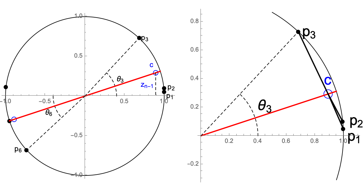
Figure 9. A perturbation of the degenerate rotating state of six particles into a non-degenerate rotating state. The particles naturally split into two groups, one appearing on the left and one appearing on the right of the picture. The center of mass for each group is depicted as a hollow circle on the slanted center (red solid) line. These centers are polar opposites of each other. The $y$-coordinate of the center of mass of the right group is given by the variable $z_{n-1}$. The variables $\theta$’s introduced above measure the perturbation of the polar angles relative to the $x$-axis. The quantity $\mathcal{D}_{L}=|p_{3}-c|^{2}+|p_{2}-c|^{2}+|p_{1}-c|^{2}$ captures the dispersion of the right group and will be used below as a Lyapunov function in the proof of stability.

In the following lemma, we describe some of the equilibrium points for (34). In what follows by “small enough” we mean vectors $Z$ for which the functions $\mathcal{E}(Z)$ and $\alpha(Z)$ are well-defined.

Lemma 5.6.

Suppose $Z_{0}\in\mathbb{R}^{n-1}$ is small enough with $\mathcal{E}(Z_{0})=0$. Then the point $(Z_{0},\alpha(Z_{0}),\mathbf{0}_{n-1},\mathbf{0}_{n-1},0,0)$ is a stationary point for the reduced flow (34).

Proof.

Let $P=(Z_{0},\alpha(Z_{0}),\mathbf{0}_{n-1},\mathbf{0}_{n-1},0,0)$. Substituting $Z=Z_{0}$, $\beta=\alpha(Z_{0})$, $\beta_{\Diamond}=\beta_{\ast}=\mathbf{0}_{n-1}$, $\gamma_{1}=\gamma_{2}=0$ in $\mathbb{c}$ and $\mathbb{s}$ from (29), we get that

$$\mathbb{c}=\mathbb{V}\alpha(Z_{0})=\mathbb{V}\alpha(Z_{0})+\mathcal{E}(Z_{0})X=\cos(\Theta)-\mathbf{1}_{n}\mbox{ and }\mathbb{s}=-\mathbb{V}Z_{0}=-\sin(\Theta).$$

Hence,

$$(\mathbb{c}_{k}+1)^{2}+\mathbb{s}_{k}^{2}-1=(\cos\theta_{k})^{2}+(-\sin\theta_{k})^{2}-1=0.$$

It follows from (23) that $\mathcal{U}_{k}=0$ and $\mathcal{W}_{k}=2\mathbb{c}_{k}$ at the point $P$. Note that at $P$ we have that

$$\mathbb{T}\mathcal{W}=\mathbb{T}(2\mathbb{c})=2\mathbb{T}(\cos(\Theta)-\mathbf{1}_{n})=2\mathbb{T}\cdot\mathbb{V}\alpha(Z_{0})=2\alpha(Z_{0}),$$

where the last equality follows from the fact that $\mathbb{T}\mathbb{V}=\textrm{I}_{n-1}$, see Section (5.2) for details. Similarly,

$$X^{T}\mathcal{W}=X^{T}(2\mathbb{c})=2X^{T}\mathbb{V}\alpha(Z_{0})=0.$$

Thus, substituting the point $P$ into the RHS of (34), we obtain

$$\left[\begin{array}[]{cccc}\textrm{O}_{n-1,n-1}&&&\\ &J_{top}&&\\ &&-1&1\\ &&0&-1\\ \end{array}\right]\left[\begin{array}[]{c}Z_{0}\\ \left[\begin{array}[]{l}\alpha(Z_{0})\\ \mathbf{0}_{n-1}\\ \mathbf{0}_{n-1}\end{array}\right]\\ 0\\ 0\\ \end{array}\right]+\left[\begin{array}[]{c}\mathbf{0}_{n-1}\\ \left[\begin{array}[]{l}\mathbf{0}_{n-1}\\ \mathbf{0}_{n-1}\\ 2\alpha(Z_{0})\end{array}\right]\\ 0\\ 0\end{array}\right]$$

It follows from (31) that $J_{top}\cdot(\alpha(Z_{0}),\mathbf{0}_{n-1},\mathbf{0}_{n-1})^{T}=(\mathbf{0}_{n-1},\mathbf{0}_{n-1},-2\alpha(Z_{0}))$. Thus, the RHS of (34) vanishes at the point $P$, whereby establishing that $P$ is an equilibrium point for the reduced system (34). ∎

Remark 5.7.

(1) Since every centre manifold $\mathcal{M}$ must contain all nearby stationary points of the flow, in view of Lemma 5.6, the points $(Z,\alpha(Z),\mathbf{0}_{n-1},\mathbf{0}_{n-1},0,0)$ with $\mathcal{E}(Z)=0$ belong to the centre manifold.

(2) Additionally, since $\mathcal{M}$ can be locally represented by the graph of a function $h:\mathbb{R}^{n-1}\rightarrow\mathbb{R}^{3n-1}$, if $Y=h(Z)$ and $\mathcal{E}(Z)=0$, then $Y=(\alpha(Z),\mathbf{0}_{n-1},\mathbf{0}_{n-1},0,0)$, that is, $(Z,Y)$ is a fixed point of the reduced flow. In other words, the set $\{(Z,Y)\in\mathcal{M}:\mathcal{E}(Z)=0\}$ consists of fixed points and, thus, is flow-invariant.

(3) Given a point on the centre manifold with initial value $\mathcal{E}(Z)>0,$ we have $\mathcal{E}(Z(t))>0$ for all $t$ for which $\mathcal{E}(Z(t))$ is defined. A similar result holds for negative values of $\mathcal{E}$.

(4) In view of Lemmas 3.1 and 5.6, points of the center manifold satisfying $\mathcal{E}(Z)=0$ represent rotating states of the original system (1).

In the main result of this subsection, the Approximation Theorem (Theorem 5.9), we construct an approximation for the flow on the center manifold of the reduced system (34). In the proof we approximate the center manifold as $\mathcal{M}=\{Q_{Z}\}$ where $Q_{Z}$ is semi-explicitly defined in (41). In our construction, we extensively exploit the fact that the set of fixed points is “large” and known within the center manifold as witnessed by Lemma 5.6. The fixed points are described via $\alpha(Z)$ and thus through the angles $\Theta(Z)$. Our next result, Lemma 5.8, quantifies the dispersion of $\sin(\Theta)$ and $\cos(\Theta)$ from their own averages ($z_{n-1}$ and $\mathcal{A}(Z)$, respectively) and will be needed to track down the scale of errors made in calculating the orbits of the contraction operator. It will be important later on to compare the errors not just to $|Z|$, but to the smaller $|Z|_{r};$ that refinement motivates next Lemma.

Notation: In what follows $\mathcal{O}(f(x))$ will stand for the standard big-O notation as $x\to 0$ and “$\odot$” will denote the Hadamard (component wise) product of vectors.

We refer the reader to Definition 5.3 for the concepts and notations pertaining to the statement and the proof of the following lemma and approximation theorem.

Lemma 5.8.

For small $Z\in\mathbb{R}^{n-1}$ we have

1. $\sin(\Theta)=\mathcal{O}(|Z|)$,

2. $\sin(\Theta)-z_{n-1}\mathbf{1}_{n}=\mathcal{O}(|Z|_{r})$,

3. $\sin^{2}(\Theta)-z^{2}_{n-1}\mathbf{1}_{n}=\mathcal{O}(|Z|_{r}|Z|)$,

4. $\mathcal{E}(Z)=\mathcal{O}(|Z|_{r}|Z|)$,

5. $\cos(\Theta)=\mathcal{A}(Z)\mathbf{1}_{n}+\mathcal{O}(|Z|_{r}|Z|)$.

Proof.

Recall that $\sin(\Theta)=\mathbb{V}Z$. Hence, $|\sin(\Theta)|=\mathcal{O}(|Z|)$. Additionally, $\sin(\Theta_{U})=VZ_{U}+z_{n-1}\mathbf{1}_{N}$ and $\sin(\Theta_{L})=VZ_{L}+z_{n-1}\mathbf{1}_{N}$. Hence, $\sin(\Theta)-z_{n-1}\mathbf{1}_{n}=\mathcal{O}(|Z|_{r})$, which, in particular, implies that $\sin^{2}(\Theta)-z^{2}_{n-1}\mathbf{1}_{n}=\mathcal{O}(|Z|_{r}|Z|)$.

Using the triangle inequality, we get that

$$|\sin(\theta_{i})-\sin(\theta_{j})|\leq|\sin(\theta_{i})-z_{n-1}|+|\sin(\theta_{j})-z_{n-1}|\leq|VZ_{U}|+|VZ_{L}|=\mathcal{O}(|Z|_{r}).$$

Now we need the following fact: $\frac{d}{dt}\sqrt{1-t^{2}}=\mathcal{O}(t)$. Applying the mean value theorem to the function $\sqrt{1-t^{2}}$, we obtain that

$$|\cos(\theta_{i})-\cos(\theta_{j})|=|\sqrt{1-\sin^{2}(\theta_{i})}-\sqrt{1-\sin^{2}(\theta_{j})}|\\ =\mathcal{O}(|\sin(\Theta)|)|\sin(\theta_{i})-\sin(\theta_{j})|=\mathcal{O}(|Z|_{r}|Z|).$$

It follows that

$$\cos(\theta_{k})-\mathcal{A}(Z)=\frac{1}{n}\sum_{m=1}^{n}(\cos(\theta_{k})-\cos(\theta_{m}))=\mathcal{O}(|Z|_{r}|Z|).$$

Similarly,

$$\mathcal{E}(Z)=\frac{1}{n}\sum_{m=1}^{N}(\cos(\theta_{m})-\cos(\theta_{N+m}))=\mathcal{O}(|Z|_{r}|Z|).$$

∎

Theorem 5.9 (The Approximation Theorem).

Let $\mathcal{M}$ be the local center manifold for the reduced flow (34). In a neighborhood of the origin, (i) the projection of the flow on $\mathcal{M}$ onto the neutral directions satisfies

$$\frac{dZ}{dt}=\mathcal{E}(Z)\mathcal{A}(Z)\left[\begin{array}[]{c}Z_{U}\\ -Z_{L}\\ 0\end{array}\right]+\mathcal{E}(Z)\mathcal{O}(|Z|_{r}|Z|)\mathbf{1}_{n-1};$$

(ii) the projection of the flow on $\mathcal{M}$ onto the $\gamma=(\gamma_{1},\gamma_{2})$ coordinates satisfies

$$\frac{d\gamma}{dt}=\mathcal{E}(Z)\mathcal{O}(|Z|_{r}).$$

Proof.

(I) For small enough $Z\in\mathbb{R}^{n-1}$, define $Q_{Z}\in\mathbb{R}^{4n-2}$ as:

$$Q_{Z}=\left[Z,\alpha(Z),\mathbf{0}_{n-1},\mathbf{0}_{n-1},\mathcal{E}(Z)f_{1}(Z),\mathcal{E}(Z)(2-f_{1}(Z)+f_{2}(Z))\right]^{T},$$ (41)

where the functions $f_{1}(Z),f_{2}(Z)$ are defined as (the unique) scalar-valued functions that solve the system of linear equations

$$\begin{split}-(1+f_{1})\left(\frac{1}{n}\mathbf{1}_{n}^{T}\cdot\sin(2\Theta)\right)-(2+f_{2})\left(\frac{2}{n}\mathbf{1}_{n}^{T}\cdot\sin^{2}(\Theta)\right)&=f_{1}\\ 2(1+f_{1})\left(\frac{1}{n}\mathbf{1}_{n}^{T}\cdot\cos^{2}(\Theta)\right)+(2+f_{2})\left(\frac{1}{n}\mathbf{1}_{n}^{T}\cdot\sin(2\Theta)\right)&=2+f_{2}.\end{split}$$ (42)

Note that in the special case when $Z=\mathbf{0}_{n-1}$ the linear system that defines $f_{1}$ and $f_{2}$ is nonsingular with solution $f_{1}(\mathbf{0}_{n-1})=0$ and $f_{2}(\mathbf{0}_{n-1})=0,$ thus, the functions $f_{1}$ and $f_{2}$ are well-defined and small, $f_{i}(Z)=\mathcal{O}(Z)$, for all small enough $Z$. An explanation of why $Q_{Z}$ is defined this way is given in Remark 5.11.

Our first goal is to show that the center manifold $\mathcal{M}$ can be locally approximated by $\{Q_{Z}:Z\in\mathbb{R}^{n-1}\}.$ We then use the explicit form of $Q_{Z}$ to approximate the RHS of (34) and to obtain an approximation for the flow on $\mathcal{M}$. Observe that for every $Z$, the constant function $Q_{Z}$ belongs to the space of slow-growing functions $\mathcal{F}_{\eta}$. We also mention that all the functions appearing in this proof are analytic with respect to $Z$.

Lemma 5.10.

For small enough $Z\in\mathbb{R}^{n-1}$, $||\Gamma_{Z}(Q_{Z})-Q_{Z}||_{\eta}=\mathcal{E}(Z)\mathcal{O}(|Z|_{r})$.

Proof of the lemma. In view of (39), the proof relies on finding appropriate approximations for $T\mathcal{U}(Q_{Z})$, $T\mathcal{W}(Q_{Z})$, $X^{T}\cdot\mathcal{U}(Q_{Z})$, and $X^{T}\cdot\mathcal{W}(Q_{Z})$.

From (29) and (41), we get that

$$\mathbb{c}=\mathbb{V}\alpha(Z)-\mathcal{E}(Z)f_{1}(Z)X\mbox{ and }\mathbb{s}=-\mathbb{V}Z+\mathcal{E}(Z)(2+f_{2}(Z)).$$

To simplify the notation, we will omit the argument in the functions $\mathcal{E}$ and $f_{1}$, $f_{2}$. Using Definition (5.3), we get

$$\mathbb{c}+\mathbf{1}_{n}=\cos(\Theta)-(1+f_{1})\mathcal{E}X\mbox{ and }\mathbb{-s}=\sin(\Theta)-\mathcal{E}(2+f_{2})X.$$

Simplify

$$(\mathbb{c}+\mathbf{1}_{n})^{2}+\mathbb{s}^{2}-\mathbf{1}_{n}=\mathcal{E}^{2}(1+f_{1})^{2}\mathbf{1}_{n}-2\mathcal{E}(1+f_{1})\cos(\Theta)\odot X+\mathcal{E}^{2}(2+f_{2})^{2}\mathbf{1}_{n}\\ -2\mathcal{E}(2+f_{2})\sin(\Theta)\odot X.$$

Recall that according to Lemma 5.8, we have that $\sin(\Theta)=\mathcal{O}(|Z|)$ and $\mathcal{E}(Z)=\mathcal{O}(|Z|_{r}|Z|)$. Also $f_{i}(Z)=\mathcal{O}(|Z|)$. Therefore,

$$(\mathbb{c}+\mathbf{1}_{n})^{2}+\mathbb{s}^{2}-\mathbf{1}_{n}=\mathcal{E}\big{[}-2(1+f_{1})\cos(\Theta)\odot X-2(2+f_{2})\sin(\Theta)\odot X+\mathcal{O}(|Z|_{r}|Z|)\big{]}$$ (43)

and

$$-\mathbb{s}=\sin(\Theta)+\mathcal{O}(|Z|_{r}|Z|).$$

From (23), we get that

$$\begin{split}\mathcal{U}&=-\mathbb{s}\left((\mathbb{c}+1)^{2}+\mathbb{s}^{2}-1)\right)\\ &=\mathcal{E}\left[-2(1+f_{1})\cos(\Theta)\odot\sin(\Theta)\odot X-2(2+f_{2})\sin^{2}(\Theta)\odot X+\mathcal{O}(|Z|_{r}|Z|)\right]\\ &=\mathcal{E}\left[-(1+f_{1})\sin(2\Theta)\odot X-2(2+f_{2})\sin^{2}(\Theta)\odot X+\mathcal{O}(|Z|_{r}|Z|)\right].\end{split}$$ (44)

Therefore, using (42) we get that

$$\begin{split}\frac{1}{n}X^{T}\cdot\mathcal{U}&=\mathcal{E}\left[-\frac{1}{n}\mathbf{1}_{n}^{T}\cdot\sin(2\Theta)(1+f_{1})-\frac{2}{n}\cdot\mathbf{1}_{n}^{T}\cdot\sin^{2}(\Theta)(2+f_{2})+\mathcal{O}(|Z|_{r}|Z|)\right]\\ &=\mathcal{E}f_{1}+\mathcal{E}\mathcal{O}(|Z|_{r}|Z|).\end{split}$$ (45)

From Lemma (5.8),

$$\cos(\Theta)\sin(\Theta)=\mathcal{A}(Z)\sin(\Theta)+\mathcal{O}(|Z|_{r}|Z|)\mbox{ and }\sin^{2}(\Theta)=z_{n-1}^{2}\mathbf{1}_{n}+\mathcal{O}(|Z|_{r}|Z|).$$

Thus, Equation (44) becomes

$$\mathcal{U}=\mathcal{E}\left[-2(1+f_{1})\mathcal{A}(Z)\sin(\Theta)\odot X-2(2+f_{2})z_{n-1}^{2}X+\mathcal{O}(|Z|_{r}|Z|)\right]$$ (46)

Recall that the matrix $\mathbb{T}$ was defined as the top $n-1$ rows of the matrix $[\mathbb{V},X]^{-1}$ and that we denoted by $T$ the top $N-1$ rows of the matrix $[V,\mathbf{1}_{N}]^{-1}$. Using the block-structure of the matrix $\mathbb{V}$ from (26), we had that

$$\textrm{col}[\mathbb{V},X]^{-1}=\left[\begin{array}[]{cc}T&\textrm{O}_{N-1,N}\\ \textrm{O}_{N-1,N}&T\\ \frac{1}{2N}\mathbf{1}_{N}^{T}&\frac{1}{2N}\mathbf{1}_{N}^{T}\\ \frac{1}{2N}\mathbf{1}_{N}^{T}&-\frac{1}{2N}\mathbf{1}_{N}^{T}\end{array}\right]\;\mbox{ and }\;\mathbb{T}=\left[\begin{array}[]{cc}T&\textrm{O}_{N-1,N}\\ \textrm{O}_{N-1,N}&T\\ \frac{1}{2N}\mathbf{1}_{N}^{T}&\frac{1}{2N}\mathbf{1}_{N}^{T}\end{array}\right].$$

Using the fact that $TV=\mathbf{1}_{N-1}$ and $T\mathbf{1}_{N}=\mathbf{0}_{N-1}$, we get that

$$\mathbb{T}\cdot(\sin(\Theta)\odot X)=\left[\begin{array}[]{cc}T&\textrm{O}_{N-1,N}\\ \textrm{O}_{N-1,N}&T\\ \frac{1}{2N}\mathbf{1}_{N}^{T}&\frac{1}{2N}\mathbf{1}_{N}^{T}\end{array}\right]\cdot\left[\begin{array}[]{c}VZ_{U}+z_{n-1}\mathbf{1}_{N}\\ -VZ_{L}-z_{n-1}\mathbf{1}_{N}\end{array}\right]=\left[\begin{array}[]{c}Z_{U}\\ -Z_{L}\\ 0\end{array}\right].$$

Note also that $\mathbb{T}\cdot X=\mathbf{0}_{n}$. Thus, using (46), we obtain that

$$\begin{split}\mathbb{T}\mathcal{U}&=2\mathcal{E}(1+f_{1})\mathcal{A}(Z)\left[\begin{array}[]{c}-Z_{U}\\ Z_{L}\\ 0\end{array}\right]+\mathcal{E}O(|Z|_{r}|Z|)\\ &=2\mathcal{E}\mathcal{A}(Z)\left[\begin{array}[]{c}-Z_{U}\\ Z_{L}\\ 0\end{array}\right]+2\mathcal{E}f_{1}\mathcal{A}(Z)\left[\begin{array}[]{c}-Z_{U}\\ Z_{L}\\ 0\end{array}\right]+\mathcal{E}O(|Z|_{r}|Z|)\\ &=2\mathcal{E}\mathcal{A}(Z)\left[\begin{array}[]{c}-Z_{U}\\ Z_{L}\\ 0\end{array}\right]+\mathcal{E}\mathcal{O}(|Z|_{r}|Z|).\end{split}$$ (47)

We now pursue similar approximations for $\mathcal{W}$. Recall that

$$\mathcal{W}=-(\mathbb{c}+\mathbf{1}_{n})\left((\mathbb{c}+\mathbf{1}_{n})^{2}+\mathbb{s}^{2}-\mathbf{1}_{n}\right)+2\mathbb{c}.$$

The term $2\mathbb{c}=2\mathbb{V}\alpha-2\mathcal{E}f_{1}X$ contributes

$$\mathbb{T}(2\mathbb{c})=2\mathbb{T}\mathbb{V}\alpha-2\mathcal{E}f_{1}\mathbb{T}X=2\alpha\mathbf{1}_{n-1}\mbox{ and }\frac{1}{n}X^{T}(2\mathbb{c})=-2\mathcal{E}f_{1}.$$ (48)

Our goal is to show that $-(\mathbb{c}+\mathbf{1}_{n})\left((\mathbb{c}+\mathbf{1}_{n})^{2}+\mathbb{s}^{2}-\mathbf{1}_{n}\right)$ gives $\mathcal{E}\mathcal{O}(|Z|_{r})$ when multiplied by $\mathbb{T}$, and that it gives $\mathcal{E}(2+f_{2})+\mathcal{E}\mathcal{O}(|Z|_{r}|Z|)$ when multiplied by $\frac{1}{n}X^{T}.$

Combining Equation (43) and the fact $(-1)(\mathbb{c}+\mathbf{1}_{n})=-\cos(\Theta)+(1+f_{1})\mathcal{E}X=-\cos(\Theta)+\mathcal{O}(|Z|_{r}|Z|)$, we obtain that

$$\mathcal{W}-2c=\mathcal{E}\left[2(1+f_{1})\cos^{2}(\Theta)\odot X+(2+f_{2})\sin(2\Theta)\odot X+\mathcal{O}(|Z|_{r}|Z|)\right].$$

Thus, from the second equation of the system (42) defining $f_{1},f_{2}$ :

$$\begin{split}\frac{1}{n}X^{T}\cdot(\mathcal{W}-2\mathbb{c})&=\mathcal{E}\left[2(1+f_{1})\frac{1}{n}\mathbf{1}_{n}^{T}\cos^{2}(\Theta)+\frac{1}{n}\mathbf{1}_{n}^{T}(2+f_{2})\sin(2\Theta)+\mathcal{O}(|Z|_{r}|Z|)\right]\\ &=\mathcal{E}\left[2+f_{2}+\mathcal{O}(|Z|_{r}|Z|)\right]\end{split}$$

and, using $\cos(\Theta)=\mathcal{A}(Z)+\mathcal{O}(|Z|_{r}|Z|)$,

$$\begin{split}\mathbb{T}(\mathcal{W}-2\mathbb{c})&=\mathbb{T}\mathcal{E}\left[2(1+f_{1})\mathcal{A}^{2}(Z)X+2(2+f_{2})\mathcal{A}(Z)\sin(\Theta)\odot X+\mathcal{O}(|Z|_{r}|Z|).\right]\\ &=0+2(2+f_{2})\mathcal{E}\mathcal{A}(Z)\left[\begin{array}[]{c}Z_{U}\\ -Z_{L}\\ 0\end{array}\right]+\mathcal{E}\mathcal{O}(|Z|_{r}|Z|)\\ &=\mathcal{E}\mathcal{O}(|Z|_{r}).\end{split}$$

Combining these equations with (48), we obtain that

$$\begin{split}\frac{1}{n}X^{T}\cdot\mathcal{W}&=\mathcal{E}(2-2f_{1}+f_{2})+\mathcal{E}\mathcal{O}(|Z|_{r}|Z|)\\ \mathbb{T}\mathcal{W}&=2\alpha(Z)\mathbf{1}_{n-1}+\mathcal{E}\mathcal{O}(|Z|_{r}).\end{split}$$ (49)

It follows from (47) that $\mathbb{T}\mathcal{U}=\mathcal{E}\mathcal{O}(|Z|_{r})$. Using it along with Equations (45) and (49) in Equation (39), which defines the contraction operator $\Gamma_{Z}$, we obtain that

$$\begin{split}\Gamma_{Z}(Q_{Z})(t)&=\left(\begin{array}[]{c}Z-\frac{t}{2}\mathbb{T}\mathcal{U}(Q_{Z})\\ \frac{1}{2}(\mathbb{T}\mathcal{U}(Q_{Z})+\mathbb{T}\mathcal{W}(Q_{Z}))\\ 0_{n-1}\\ -\frac{1}{2}\mathbb{T}\mathcal{U}(Q_{Z})\\ \frac{1}{n}X^{T}\mathcal{U}(Q_{Z})\\ \frac{1}{n}X^{T}(\mathcal{U}(Q_{Z})+\mathcal{W}(Q_{Z}))\end{array}\right)\\ &=\left(\begin{array}[]{c}Z+\mathcal{E}\mathcal{O}(|Z|_{r})\\ \alpha(Z)+\mathcal{E}\mathcal{O}(|Z|_{r})\\ 0_{n-1}\\ \mathcal{E}\mathcal{O}(|Z|_{r})\\ \mathcal{E}f_{1}+\mathcal{E}\mathcal{O}(|Z|_{r}|Z|)\\ \mathcal{E}f_{1}+\mathcal{E}(2-2f_{1}+f_{2})+\mathcal{E}\mathcal{O}(|Z|_{r}|Z|)\end{array}\right)\\ &=Q_{Z}+\mathcal{E}\mathcal{O}(|Z|_{r}),\end{split}$$ (50)

which completes the proof of the lemma. $\hfill\square$

In the space $\mathcal{F}_{\eta}$ of slow-growing functions, the operator $\Gamma_{Z}$ contracts with a rate of $1/2$, see [2, (3.7)]. It follows from the contraction mapping theorem that the fixed point function $F_{Z}(t)$ and the constant function $Q_{Z}$ satisfy

$$||F_{Z}(t)-Q_{Z}||_{\eta}\leq\frac{1}{1-\frac{1}{2}}||\Gamma_{Z}(Q_{Z})-Q_{Z}||_{\eta}=\mathcal{E}(Z)\mathcal{O}(|Z|_{r}),$$

where the $\eta$-norm is defined in (37). We also have that

$$|F_{Z}(0)-Q_{Z}|\leq||F_{Z}(t)-Q_{Z}||_{\eta}=\mathcal{E}(Z)\mathcal{O}(|Z|_{r}).$$ (51)

The center manifold theorem [2] states that the set $\mathcal{M}=\{F_{Z}(0)\}$, when $Z$ runs over a small neighborhood of the origin in $\mathbb{R}^{n-1}$, is a center manifold of the system. The stable variables of $\mathcal{M}$ are quadratic, $\mathcal{O}(|Z|^{2})$, in $Z$. Since by (29), $\mathbb{c}=\mathbb{V}\beta+\mathbb{V}\beta_{\ast}-\gamma_{1}X$ and $\mathbb{s}=-\mathbb{V}Z+\frac{1}{2}V\beta_{\Diamond}+(\gamma_{1}+\gamma_{2})$, we obtain that $\mathbb{c}=\mathcal{O}(|Z|^{2})$ and $\mathbb{s}=\mathcal{O}(|Z|)$ when evaluated at $F_{Z}(0)\in\mathcal{M}$. It follows from (51) that $\mathbb{s}=\mathcal{O}(|Z|)$ and $\mathbb{c}=\mathcal{O}(|Z|)$ along any line segment connecting $F_{Z}(0)$ and $Q_{Z}$.

Therefore, calculating the gradient of the function $\mathcal{U}_{k}$, we obtain that $|\nabla\mathcal{U}_{k}|\leq 2|\mathbb{s}_{k}\mathbb{c}_{k}|+2|\mathbb{s}|+|\mathbb{c}_{k}|^{2}+2|\mathbb{c}_{k}|+3|\mathbb{s}_{k}^{2}|=\mathcal{O}(|Z|)$ along the line segment connecting $F_{Z}(0)$ and $Q_{Z}$. It follows from the mean value theorem that

$$|\mathcal{U}(F_{Z}(0))-\mathcal{U}(Q_{Z})|\leq\mbox{max}|\nabla\mathcal{U}|\cdot|F_{Z}(0)-Q_{Z}|=\mathcal{O}(|Z|)\mathcal{E}\mathcal{O}(|Z|_{r})=\mathcal{E}(Z)\mathcal{O}(|Z|_{r}|Z|).$$ (52)

Combining (52) with (47), we obtain that

$$\frac{dZ}{dt}\Big{|}_{F_{Z}(0)}=-\frac{1}{2}\mathbb{T}\mathcal{U}(F_{Z}(0))=\mathcal{E}(Z)\mathcal{A}(Z)\left[\begin{array}[]{c}Z_{U}\\ -Z_{L}\\ 0\end{array}\right]+\mathcal{E}(Z)\mathcal{O}(|Z|_{r}|Z|),$$

which completes the proof of the first part of the theorem.

(II) Our next goal is to obtain estimates for $(\dot{\gamma}_{1},\dot{\gamma}_{2})$ for the flow on the center manifold. Recall that

$$\left(\begin{array}[]{c}\dot{\gamma}_{1}\\ \dot{\gamma}_{2}\end{array}\right)=\left[\begin{array}[]{cc}-1&1\\ 0&-1\end{array}\right]\left(\begin{array}[]{c}\gamma_{1}\\ \gamma_{2}\end{array}\right)+\left(\begin{array}[]{l}-\frac{1}{n}X^{T}\cdot\mathcal{W}\\ \frac{1}{n}X^{T}\cdot(\mathcal{U}+\mathcal{W})\end{array}\right).$$ (53)

Fix $Z\in\mathbb{R}^{n-1}$ and consider $Q_{Z}$ and the corresponding point $F_{Z}(0)$ on the center manifold. Recall that $\gamma_{1}|_{Q_{Z}}=\mathcal{E}f_{1}$ and $\gamma_{2}|_{Q_{Z}}=\mathcal{E}(2-f_{1}+f_{2}).$ It follows from (51) and the structure of $Q_{Z}$ that

$$\gamma_{1}|_{F_{Z}(0)}=\mathcal{E}f_{1}+\mathcal{E}\mathcal{O}(|Z|_{r})\mbox{ and }\gamma_{2}|_{F_{Z}(0)}=2\mathcal{E}-\mathcal{E}f_{1}+\mathcal{E}f_{2}+\mathcal{E}\mathcal{O}(|Z|_{r}).$$ (54)

From (45), we get that $\frac{1}{n}X^{T}\cdot\mathcal{U}(Q_{Z})=\mathcal{E}f_{1}+\mathcal{E}\mathcal{O}(|Z|_{r})$. Combining it with (52), we obtain that

$$\frac{1}{n}X^{T}\cdot\mathcal{U}(F_{Z}(0))=\mathcal{E}f_{1}+\mathcal{E}\mathcal{O}(|Z|_{r}).$$ (55)

Using arguments similar to those preceding Equation (52), we obtain that $|\nabla\mathcal{W}|=\mathcal{O}(|Z|)$ along any line segment connecting $Q_{Z}$ and $F_{Z}(0)$. Thus, using the mean value theorem we obtain that

$$|\mathcal{W}(F_{Z}(0))-\mathcal{W}(Q_{Z})|\leq\mbox{max}|\nabla\mathcal{W}|\cdot|F_{Z}(0)-Q_{Z}|=\mathcal{O}(|Z|)\mathcal{E}\mathcal{O}(|Z|_{r})\\ =\mathcal{E}(Z)\mathcal{O}(|Z|_{r}|Z|).$$

Combining this estimate with (49), we obtain that

$$\frac{1}{n}X^{T}\cdot\mathcal{W}(F_{Z}(0))=2\mathcal{E}-2\mathcal{E}f_{1}+\mathcal{E}f_{2}+\mathcal{E}\mathcal{O}(|Z|_{r}).$$ (56)

Substituting (54), (55), and (56) into (53), we obtain that

$$\dot{\gamma}_{1}|_{F_{Z}(0)}=\mathcal{E}(Z)\mathcal{O}(|Z|_{r})\mbox{ and }\dot{\gamma}_{2}|_{F_{Z}(0)}=\mathcal{E}(Z)\mathcal{O}(|Z|_{r}),$$

which completes the proof of the theorem. ∎

Remark 5.11.

The Approximation Theorem rests on the fact that the central manifold $\mathcal{M}=\{F_{Z}(0)\}$, when $Z$ runs over a small neighborhood of the origin in $\mathbb{R}^{n-1}$, is well approximated by $\mathcal{M}=\{Q_{Z}\},$ thus the central manifold is approximated by the graph of the function $Z\to\left[\alpha(Z),\mathbf{0}_{n-1},\mathbf{0}_{n-1},\mathcal{E}(Z)f_{1}(Z),\mathcal{E}(Z)(2-f_{1}(Z)+f_{2}(Z))\right]^{T}.$ We emphasize that the function $\alpha(Z)$ has an infinite Taylor series expansion. Thus, had we truncated it to a Taylor polynomial, we would have missed the stationary points of the form $(Z_{0},\alpha(Z_{0}),\mathbf{0}_{n-1},\mathbf{0}_{n-1},0,0)$ where $\mathcal{E}(Z_{0})=0,$ described in Lemma 5.6. The motivation for the point $Q_{Z}$ comes from the approximation method detailed in the Appendix. We include a brief summary here, for the sake of completeness.

For a given $Z,$ we shadow the orbit $\Gamma^{k}_{Z}(y)$ for $k=1,2,\dots,$ of some constant function $y=y(Z).$ The orbit converges to the fixed point of $\Gamma_{Z};$ for the shadow orbit we keep track of the accrued errors. Ideally we would like to use the solution $[\beta,\beta_{\Diamond},\beta_{\ast},\gamma_{1},\gamma_{2}]$ to $\dot{\beta}=0$, $\dot{\beta}_{\Diamond}=0$, $\dot{\beta}_{\ast}=0$, $\dot{\gamma}_{1}=0$, and $\dot{\gamma}_{2}=0$, from (34) as the staring value for $y(Z)$, but, unfortunately, there is no closed-form explicit description of the solution. Instead, we use stationary points as our starting approximations.

Note that for any $Z$ with $\mathcal{E}(Z)=0$, the function $y_{0}=(Z,\alpha(Z),\mathbf{0}_{n-1},\mathbf{0}_{n-1},0,0)$ is the actual fixed point of the operator $\Gamma_{Z}$. Inspired by this observation, for any $Z$, we still use the aforementioned $y_{0}$ as the initial point for the operator $\Gamma_{Z}$. We get that $\Gamma_{Z}(y_{0})$ satisfies

$$\Gamma_{Z}(y_{0})(t)=y_{0}+\mathcal{E}(Z)\mbox{col}[[-tZ_{U},tZ_{L},0],\mathbf{0}_{3n-3},0,2]+\mathcal{E}(Z)\mathcal{O}(|Z|),$$

which can be verified using the arguments from Theorem 5.9 and Lemma 5.10. We are looking for a pseudo-orbit consisting of constant functions that are within $\mathcal{E}(Z)\mathcal{O}(|Z|)$ from the true iterates. Thus, we eliminate the first-degree in $t$ and all $\mathcal{E}(Z)\mathcal{O}(|Z|)$ terms and define the next constant function as
$y_{1}=(Z,\alpha(Z),\mathbf{0}_{n-1},\mathbf{0}_{n-1},0,2\mathcal{E}(Z)).$ Once more, we compute $\Gamma_{Z}(y_{1})(t)$ and compare it to $y_{1}.$ The error estimates are sharper, but those associated with the last two components $(\gamma_{1},\gamma_{2})$ are inferior to those obtained in the first $4n-4$ components in the sense that they are of the type $\mathcal{E}(Z)\mathcal{O}(|Z|^{2})$ whereas the errors of the other $4n-4$ components are $\mathcal{E}(Z)\mathcal{O}(|Z|)\mathcal{O}(|Z|_{r}).$

We shadow $\Gamma_{Z}(y_{1})(t)$ by $y_{2}=y_{2}(Z)$ using $y_{2}=y_{1}+(\mathbf{0}_{n-1},\mathbf{0}_{3n-3},g_{1}\mathcal{E}(Z),g_{2}\mathcal{E}(Z)),$ where the functions $g_{1},g_{2}$ are (implicitly) defined such that the last two components of $y_{2}$ and of $\Gamma_{Z}(y_{2})$ coincide up to $\mathcal{E}(Z)\mathcal{O}(|Z|_{r}).$ The extra precision requirement is satisfied when $(g_{1},g_{2})$ solve a linear system similar to that in (42), specifically when $g_{1}=f_{1}$ and $g_{2}=f_{2}-f_{1}$ with $f_{1},f_{2}$ being the solutions to (42). The point $Q_{Z}$ introduced in (41) and in Lemma 5.10 is the aforementioned $y_{2}.$ We highlight that the magnitude of the vector field $\frac{dZ}{dt}$ is of the order $\mathcal{E}(Z)|Z|_{r},$ which explains why we pursued that accuracy in Lemma 5.10 – stopping at $\mathcal{E}(Z)|Z|$ would not have sufficed.

5.4. Stability of the reduced flow.

In view of center manifold theory, to establish the stability of the reduced ($Z,\beta,\beta_{\Diamond},\beta_{\ast},\gamma_{1},\gamma_{2})$-system, it suffices to establish the stability of the flow on the center manifold. In fact, we will show that every solution that starts near the origin approaches an equilibrium point. Recall that in view of Lemma 3.1 and Remark 5.7, the set $\mathcal{M}\cap\{\mathcal{E}=0\}$ consists of equilibrium points of the flow, which in its turn coincides with the set of ring state solutions centered at the origin.

Theorem 5.12.

The flow on the center manifold $\mathcal{M}$ of the reduced system (34) is stable at the origin. Furthermore, any trajectory that starts near the origin approaches an equilibrium point of the form $(Z_{\omega},\alpha(Z_{\omega}),\mathbf{0}_{2n})$, $Z_{\omega}\in\mathbb{R}^{n-1}$, $\mathcal{E}(Z_{\omega})=0$.

Proof.

In view of Theorem 5.9, the flow on the center manifold is governed by

$$\frac{dZ}{dt}=\mathcal{E}(Z)\mathcal{A}(Z)\left[\begin{array}[]{c}Z_{U}\\ -Z_{L}\\ 0\end{array}\right]+\mathcal{E}(Z)\mathcal{O}(|Z|_{r}|Z|).$$

Using Remark (5.7), we notice that the sets $\mathcal{M}_{0}=\mathcal{M}\cap\{\mathcal{E}=0\}$, $\mathcal{M}_{+}=\mathcal{M}\cap\{\mathcal{E}>0\}$, and $\mathcal{M}_{-}=\mathcal{M}\cap\{\mathcal{E}<0\}$ are flow-invariant and the set $\mathcal{M}_{0}$ consists of equilibrium points. Thus, to establish stability of the flow on $\mathcal{M}$, we will separately show that the flow on $\mathcal{M}_{+}$ and $\mathcal{M}_{-}$ is stable.

Furthermore, we will prove that the flow converges towards the set $\mathcal{M}_{0}$, the set of ring states. Define the functions

$$\mathcal{D}_{U}(Z)=\frac{1}{N}(VZ_{U})^{T}\cdot VZ_{U}\mbox{ and }\mathcal{D}_{L}(Z)=\frac{1}{N}(VZ_{L})^{T}\cdot VZ_{L}.$$ (57)

Using the definition of $\sin(\Theta)$, we notice that $\mathcal{D}_{L}(Z)=\sum_{k=1}^{N}(\sin(\theta_{k})-z_{n-1})^{2}$. Furthermore, in view of Remark (5.4), $z_{n-1}=\frac{1}{N}\sum_{k=1}^{N}\sin(\theta_{k})$. Thus, $\mathcal{D}_{L}(Z)$ can be interpreted as the dispersion/scattering of the right group of particles, see also Remark (5.5) and Figure (9). Similarly, $\mathcal{D}_{U}(Z)$ can be viewed as the dispersion of the left group of particles. Given that the $N\times(N-1)$ matrix $V$ is full rank, we have that $\mathcal{D}_{U}(Z)$ and $\mathcal{D}_{L}(Z)$ are comparable with $|Z_{U}|^{2}$ and $|Z_{L}|^{2}$, respectively.

We will prove that $\mathcal{D}_{L}$ and $\mathcal{D}_{U}$ are Lyapunov functions for the flow on $\mathcal{M}_{+}$ and $\mathcal{M}_{-}$, respectively, which will ensure the stability of the flow near the origin. Finally, applying LaSalle’s Invariance Principle, we will establish the convergence of solutions to the set $\mathcal{M}_{0}$.

Notice that there is a universal constant $C>0$ such that $\sqrt{\mathcal{D}_{L}(Z)}\leq C|Z|_{r}$ and $\sqrt{\mathcal{D}_{U}(Z)}\leq C|Z|_{r}$. In the following lemma we show that $\mathcal{D}_{L}(Z)$ is comparable to $|Z|_{r}$ in $\{\mathcal{E}>0\}$ and that $\mathcal{D}_{U}(Z)$ is comparable to $|Z|_{r}$ in $\{\mathcal{E}<0\}$ for all small enough $Z$.

Lemma 5.13.

There exists a constant $C>0$ such that for all $Z$ small enough: (i) $\displaystyle\frac{1}{C}|Z|_{r}\leq\sqrt{\mathcal{D}_{L}(Z)}\leq C|Z|_{r}$ in the region where $\{\mathcal{E}>0\},$ (ii) $\displaystyle\frac{1}{C}|Z|_{r}\leq\sqrt{\mathcal{D}_{U}(Z)}\leq C|Z|_{r}$ in the region where $\{\mathcal{E}<0\}$, and (iii) $\mathcal{D}_{L}(Z)\geq\frac{1}{2}\mathcal{D}_{U}(Z)$ in $\{\mathcal{E}>0\}$.

Proof.

By definition of $\mathcal{E}$, we have that

$$\begin{split}\mathcal{E}(Z)&=\frac{1}{n}\sum_{k=1}^{N}\big{(}\cos(\theta_{k})-\cos(\theta_{N+k})\big{)}=\frac{2}{n}\sum_{k=1}^{N}\left[\sin^{2}\left(\frac{\theta_{k+N}}{2}\right)-\sin^{2}\left(\frac{\theta_{k}}{2}\right)\right]\\ &=\frac{1}{N}\sum_{k=1}^{N}\left[\sin^{2}\left(\frac{1}{2}\sin^{-1}(t_{N+k}+z_{n-1})\right)-\sin^{2}\left(\frac{1}{2}\sin^{-1}(t_{k}+z_{n-1})\right)\right],\end{split}$$

where $t_{i}=\sin(\theta_{i})-z_{n-1}$ or, equivalently, the $i$-th component of the vector $VZ_{U}$ for $1\leq i\leq N$ and of the vector $VZ_{L}$ if $N+1\leq i\leq n$.

Given a small $z\in\mathbb{R}$, consider the function $t\mapsto\sin^{2}(\frac{1}{2}\sin^{-1}(t+z))$ and its Taylor expansion of order 2 at $t=0.$ Then,

$$\sin^{2}\left(\frac{1}{2}\sin^{-1}(t+z)\right)=\sin^{2}\left(\frac{1}{2}\sin z\right)+\frac{z}{2\sqrt{1-z^{2}}}t+\frac{1}{4\sqrt{1-z^{2}}^{3}}t^{2}+R_{2}(t).$$

Expressing the remainder $R_{2}(t)$ in the Lagrange form, we can directly verify that $R_{2}(t)=t^{3}h(t,z)$, where $|h(t,z)|\leq K(|t|+|z|)$ for some constant $K>0$. Note that the constant $K$ depends only on the radius of the neighborhood of the origin.

Substituting the Taylor series expansion with $t=t_{i}$ and $z=z_{n-1}$ in the equation for $\mathcal{E}$ above, we get that

$$\mathcal{E}(Z)=\frac{1}{N}\frac{z_{n-1}}{2\sqrt{1-z_{n-1}^{2}}}\left(\sum_{k=1}^{N}t_{N+k}-\sum_{k=1}^{N}t_{k}\right)\\ +\frac{1}{N}\frac{1}{4\sqrt{1-z_{n-1}^{2}}^{3}}\left(\sum_{k=1}^{N}t_{N+k}^{2}-\sum_{k=1}^{N}t_{k}^{2}\right)+\frac{1}{N}\sum_{k=1}^{N}(R_{2}(t_{N+k})-R_{2}(t_{k})).$$ (58)

Note that $\sum_{k=1}^{N}t_{k}=\mathbf{1}_{N}^{T}VZ_{U}=0$ as the columns of the matrix $V$ are orthogonal to the vector $\mathbf{1}_{N}$. Similarly, $\sum_{k=1}^{N}t_{N+k}=0$. Note also that $\mathcal{D}_{U}=\frac{1}{N}\sum_{k=1}^{N}t_{k}^{2}$ and $\mathcal{D}_{L}=\frac{1}{N}\sum_{k=1}^{N}t_{N+k}^{2}$. Finally, observe that $h(t_{k},z_{n-1})=\mathcal{O}(|Z|)$ and $t_{k}=\mathcal{O}(|Z|_{r})=\mathcal{O}(\sqrt{\mathcal{D}_{U}+\mathcal{D}_{L}})$. Thus, continuing with Equation (58), we obtain that

$$\begin{split}\mathcal{E}(Z)&=\frac{1}{4\sqrt{1-z_{n-1}^{2}}^{3}}\left(\mathcal{D}_{L}(Z)-\mathcal{D}_{U}(Z)\right)\\ &+\frac{1}{N}\sum_{k=1}^{N}\left(t_{N+k}^{2}h(t_{N+k},z_{n-1})-t_{k}^{2}h(t_{k},z_{n-1})\right)\\ &=\frac{1}{4\sqrt{1-z_{n-1}^{2}}^{3}}\left(\mathcal{D}_{L}(Z)-\mathcal{D}_{U}(Z)\right)+(\mathcal{D}_{L}(Z)+\mathcal{D}_{U}(Z))^{3/2}H(Z),\end{split}$$ (59)

where $H(Z)=\mathcal{O}(|Z|)$. Set $f(Z)=4\sqrt{1-z_{n-1}^{2}}^{3}$. Then

$$\mathcal{D}_{U}(Z)-\mathcal{D}_{L}(Z)=-f(Z)\mathcal{E}(Z)+(\mathcal{D}_{L}(Z)+\mathcal{D}_{U}(Z))^{3/2}H(Z)f(Z).$$

Consider the case $\mathcal{E}(Z)>0$. Choose a small neighborhood of the origin in $\mathbb{R}^{n-1}$ in which $(3/2)^{3/2}\mathcal{D}_{U}(Z)^{1/2}|H(Z)|f(Z)<\frac{1}{2}$. We claim that in this neighborhood $\mathcal{D}_{L}(Z)\geq\frac{1}{2}\mathcal{D}_{U}(Z)$. Indeed, assume towards contradiction that $\mathcal{D}_{L}(Z)<\frac{1}{2}\mathcal{D}_{U}(Z)$. It follows that $\mathcal{D}_{L}(Z)-\mathcal{D}_{U}(Z)<-\frac{1}{2}\mathcal{D}_{U}(Z)$. Hence,

$$\begin{split}\frac{1}{2}\mathcal{D}_{U}(Z)&<\mathcal{D}_{U}(Z)-\mathcal{D}_{L}(Z)=-f(Z)\mathcal{E}(Z)+(\mathcal{D}_{L}(Z)+\mathcal{D}_{U}(Z))^{3/2}H(Z)f(Z)\\ &\leq(\mathcal{D}_{L}(Z)+\mathcal{D}_{U}(Z))^{3/2}H(Z)f(Z).\end{split}$$

The last inequality implies that $H(Z)>0$. It follows that

$$\frac{1}{2}\mathcal{D}_{U}(Z)<(\mathcal{D}_{L}(Z)+\mathcal{D}_{U}(Z))^{3/2}H(Z)f(Z)<\left(\frac{3}{2}\mathcal{D}_{U}(Z)\right)^{3/2}H(Z)f(Z)\leq\frac{1}{2}\mathcal{D}_{U}(Z),$$

which is a contradiction. Therefore, $|Z|_{r}=\mathcal{O}(\sqrt{\mathcal{D}_{U}+\mathcal{D}_{L}})=\mathcal{O}(\sqrt{\mathcal{D}_{L}})$ and the result follows. The proof in the case when $\mathcal{E}(Z)<0$ is similar. ∎

Lemma 5.14.

On the center manifold $\mathcal{M}$, if $Z$ is near the origin, then

$$\begin{split}\frac{d\mathcal{D}_{L}}{dt}&=-2\mathcal{E}(Z)\mathcal{A}(Z)\mathcal{D}_{L}(Z)(1+\mathcal{O}(|Z|))\mbox{ whenever }Z\in\mathcal{M}_{+}\\ \frac{d\mathcal{D}_{U}}{dt}&=2\mathcal{E}(Z)\mathcal{A}(Z)\mathcal{D}_{U}(Z)\left(1+\mathcal{O}(|Z|)\right)\mbox{ whenever }Z\in\mathcal{M}_{-}.\end{split}$$ (60)

Proof.

Consider the case when $Z\in\mathcal{M}_{+}$, that is, $\mathcal{E}(Z)>0$. In view of Lemma 5.13, $|Z|_{r}=\mathcal{O}(\sqrt{D_{L}})$. By definition, $\mathcal{D}_{L}=\frac{1}{N}(VZ_{L})^{T}\cdot VZ_{L}$. Differentiating both sides of the equation along trajectories of the flow on the center manifold and applying Theorem 5.9, we obtain that

$$\begin{split}\frac{d\mathcal{D}_{L}}{dt}&=\frac{2}{N}(VZ_{L})^{T}\cdot V\dot{Z}_{L}=-\frac{2}{N}\mathcal{E}(Z)(VZ_{L})^{T}\cdot\left[\mathcal{A}(Z)VZ_{L}+\mathcal{O}(|Z|_{r}|Z|)\right]\\ &=-2\mathcal{E}(Z)(\mathcal{A}(Z)\mathcal{D}_{L}(Z)+\mathcal{O}(|Z|_{r}^{2}|Z|))=-2\mathcal{E}(Z)\mathcal{A}(Z)\mathcal{D}_{L}(Z)(1+\mathcal{O}(|Z|)).\end{split}$$

The proof for the case $Z\in\mathcal{M}_{-}$ is analogous and will be omitted. ∎

Now we are ready to show that the flow on submanifolds $\mathcal{M}_{+}$ and $\mathcal{M}_{-}$ is stable. We will consider only $\mathcal{M}_{+}$ as the proof for $\mathcal{M}_{-}$ uses similar arguments and will be left to the reader. Recall that the submanifold $\mathcal{M}_{+}$ is flow-invariant. Lemma 5.13 implies that $\mathcal{D}_{L}(Z)>0$ for all small enough $Z\in\mathcal{M}_{+}$. Thus, it follows from Equation (60) that the function $t\mapsto\mathcal{D}_{L}(Z(t))$ is decreasing along any trajectory $Z(t)$ that stays inside $\mathcal{M}_{+}$ (the values of $\mathcal{A}(Z)$ are near $1$ for small $Z$, thus positive).

Fix any trajectory $Z(t)\subset\mathcal{M}_{+}$. Using Theorem 5.9 and the previous lemma, we differentiate the functions $\sqrt{\mathcal{D}}_{L}\pm z_{n-1}$ along $Z(t)$:

$$\begin{split}\frac{d(\sqrt{\mathcal{D}}_{L}\pm z_{n-1})}{dt}&=\frac{-2\mathcal{E}(Z)\mathcal{A}(Z)\mathcal{D}_{L}(Z)(1+\mathcal{O}(|Z|))}{2\sqrt{\mathcal{D}_{L}(Z)}}\pm\mathcal{E}(Z)\mathcal{O}(|Z|_{r}|Z|)\\ &=-2\mathcal{E}(Z)\mathcal{A}(Z)\sqrt{\mathcal{D}_{L}(Z)}(1+\mathcal{O}(|Z|))\pm\mathcal{E}(Z)\sqrt{\mathcal{D}_{L}(Z)}\mathcal{O}(|Z|)\\ &=-2\mathcal{E}(Z)\sqrt{\mathcal{D}_{L}(Z)}\mathcal{A}(Z)\left[1+\mathcal{O}(|Z|)\right],\end{split}$$

which shows that for all $Z$ small enough the functions $\sqrt{\mathcal{D}}_{L}\pm z_{n-1}$ are decreasing along trajectories in $\mathcal{M}_{+}$.

It follows from the definition of $\mathcal{D}_{L}$ and Lemma 5.13 that there are constants $C>0$ and $K>0$ such that $\sqrt{\mathcal{D}_{L}(Z)}\leq C|Z|$ and $|Z|_{r}\leq K\sqrt{\mathcal{D}_{L}(Z)}$ for all small enough $Z$. Fix an arbitrary trajectory $Z(t)=(z_{1}(t),\ldots,z_{n-1}(t))$ in $\mathcal{M}_{+}$ that starts in a small neighborhood of the origin. Since the functions $\sqrt{\mathcal{D}_{L}}$ and $\sqrt{\mathcal{D}_{L}}\pm z_{n-1}$ are decreasing along $Z(t)$, we obtain that for $t>0$:

$$\sqrt{\mathcal{D}_{L}(Z(t))}\leq\sqrt{\mathcal{D}_{L}(Z(0))}\leq C|Z(0)|$$

$$z_{n-1}(t)\leq-\sqrt{\mathcal{D}_{L}(Z(t))}+z_{n-1}(0)+\sqrt{\mathcal{D}_{L}(Z(0))}$$

$$\leq z_{n-1}(0)+\sqrt{\mathcal{D}_{L}(Z(0))}\leq(C+1)|Z(0)|$$

and

$$-z_{n-1}(t)\leq-\sqrt{\mathcal{D}_{L}(Z(t))}+\sqrt{\mathcal{D}_{L}(Z(0))}-z_{n-1}(0)$$

$$\leq\sqrt{\mathcal{D}_{L}(Z(0))}-z_{n-1}(0)\leq(C+1)|Z(0)|.$$

Thus $|z_{n-1}(t)|\leq(C+1)|Z(0)|$. It follows that

$$|Z(t)|=|Z(t)|_{r}+|z_{n-1}(t)|\leq K\sqrt{\mathcal{D}_{L}(Z(t))}+|z_{n-1}(t)|\leq(KC+C+1)|Z(0)|,$$

which establishes the stability of the system near the origin in $\mathcal{M}_{+}$ and, using similar arguments, in $\mathcal{M}_{-}$. Thus, the flow on the reduced center manifold is stable near the origin.

Finally, consider an initial condition $Z_{0}$ small enough so that for all $t>0$ its trajectory $Z(t)$ is confined to the neighborhood where the center manifold exists. Note that the existence of such a neighborhood follows from stability of the system at the origin. If $\mathcal{E}(Z_{0})=0,$ then $Z_{0}$ is a fixed point. If $\mathcal{E}(Z_{0})\neq 0,$ without loss of generality, assume $\mathcal{E}(Z_{0})>0$, that is, $Z(t)\subset\mathcal{M}_{+}$. Note that any limit point $Z_{\omega}$ of $Z(t)$ satisfies $\mathcal{E}(Z_{\omega})\geq 0.$

Applying LaSalle’s Invariance Principle to the negative semi-definite ($\dot{\mathcal{D}}_{L}\leq 0$) function $\mathcal{D}_{L}$, we obtain that $Z_{\omega}$ satisfies $\dot{\mathcal{D}}_{L}(Z_{\omega})=0$, which according to Lemma 5.14 is equivalent to $\mathcal{E}(Z_{\omega})=0$ or $\mathcal{D}_{L}(Z_{\omega})=0$. If $\mathcal{E}(Z_{\omega})=0$, then in view of Remark 5.7 the limit point $(Z_{\omega},\alpha(Z_{\omega}),\mathbf{0}_{2n})$ is an equilibrium point of the flow and the result follows. If $\mathcal{E}(Z_{\omega})>0$, then $\mathcal{D}_{L}(Z_{\omega})$ must be equal to zero. Thus, Lemma 5.13 implies that $|Z_{\omega}|_{r}=0$ and $\sin(\Theta)=z_{n-1}^{\omega}\mathbf{1}_{n-1}$, where $\Theta=\Theta(Z_{\omega})$. It follows that $\mathcal{E}(Z_{\omega})=0$, which is a contradiction. ∎

Now Theorem 5.12 and center manifold theory immediately imply the stability of the reduced system near the origin. According to [3, Theorem 2 in Section 2.4] every trajectory that starts near the origin approaches a trajectory in the center manifold $\mathcal{M}$. Since trajectories in $\mathcal{M}$ approach fixed points (ring states centered at the origin), we conclude that every trajectory of the reduced system near the origin converges to a fixed point.

Corollary 5.15.

The reduced $(Z,\beta,\beta_{\Diamond},\beta_{\ast},\gamma_{1},\gamma_{2})$-system is stable near the origin. Furthermore, each trajectory that starts near the origin approaches a fixed point of the system.

5.5. Stability of the full system.

In the full system, the coordinates $(Z,\delta_{1},\delta_{2})$ are neutral and the coordinates $(\beta,\beta_{\Diamond},\beta_{\ast},\gamma_{1},\gamma_{2})$ are stable. In this section, we establish stability of the expanded system with the variables $(\delta_{1},\delta_{2})$ being driven by the stable subsystem. Note that in the theorem below the clockwise rotation in the $\delta$ components corresponds to a translation of the center of mass of the system in the original coordinates to the limit position $(\delta_{*,1},\delta_{*,1})$. The equilibrium point $Q_{*}$ of the reduced system determines the angles of the limit configuration of the particles that in the original coordinate system rotate with unit speed about $(\delta_{*,1},\delta_{*,1})$.

Theorem 5.16.

The $(Z,\beta,\beta_{\Diamond},\beta_{\ast},\gamma_{1},\gamma_{2},\delta_{1},\delta_{2})$-system governed by (34) and (35) is stable at the origin.

Moreover, there exists a neighborhood $\mathcal{N}$ of the origin in $\mathbb{R}^{4n}$ such that the flow of (34) and (35) that starts in $\mathcal{N}$ asymptotically approaches the periodic “steady-state” oscillatory solution of the form $(Q_{*},\cos(t)\delta_{*,1}+\sin(t)\delta_{*,2},-\sin(t)\delta_{*,1}+\cos(t)\delta_{*,2}))$, where $Q_{*}$ is an equilibrium point for the reduced system (34) and $\delta_{*,1},\delta_{*,2}\in\mathbb{R}$.

Proof.

Denote by $\varphi_{t}$ the flow of the full system governed by (34) and (35). Denote by $\mathcal{M}_{n-1}$ the center manifold of the reduced system constructed in Theorem 5.9. Recall that $\mathcal{M}_{n-1}=\{F_{Z}(0):Z\in\mathbb{R}^{n-1},\;|Z|<r_{0}\}$ for some $r_{0}>0$. In view of Theorem 5.12, the flow $\varphi_{t}$ on $\mathcal{M}_{n-1}\subset\mathbb{R}^{4n-2}$ is stable near the origin. Recall also that the first $4n-2$ components of (34) decouple from the last two ($\delta_{1}$, and $\delta_{2}$). It follows that the manifold $\mathcal{M}_{n+1}=\mathcal{M}_{n-1}\times\mathbb{R}^{2}$ is (locally) forward invariant under (34) and (35), and tangent to the linear center subspace. Thus $\mathcal{M}_{n+1}$ is the center manifold for (34) and (35). In view of center manifold theory, the stability of the flow of the full system is equivalent to the stability of the flow on $\mathcal{M}_{n+1}$. Note the projection of the flow $(\mathcal{M}_{n+1},\phi_{t})$ onto $\mathbb{R}^{4n-2}$ is stable near the origin. Thus, to establish stability it suffices to show that for all initial conditions close enough to the origin, the projection of the flow $(\mathcal{M}_{n+1},\phi_{t})$ onto the $(\delta_{1},\delta_{2})$-coordinates remains close to the origin in $\mathbb{R}^{2}$ for small initial conditions from $\mathcal{M}_{n+1}$.

If $Z\in\mathbb{R}^{n-1}$ is such that $\mathcal{E}(Z)=0$, then in view of Remark 5.7, $F_{Z}(0)$ is an equilibrium point on the center manifold. It follows from the proof of Lemma 5.6 that the functions $X^{T}\cdot\mathcal{U}=0$ and $X^{T}\cdot\mathcal{W}=0$ at $F_{Z}(0)$. Therefore, using (35), we observe that whenever $(F_{Z}(0),\delta_{1},\delta_{2})\in\mathcal{M}_{n+1}$ satisfies $\mathcal{E}(Z)=0$, the flow in $(\delta_{1},\delta_{2})$ is governed by

$$\left(\begin{array}[]{c}\dot{\delta}_{1}\\ \dot{\delta}_{2}\end{array}\right)=\left(\begin{array}[]{cc}0&1\\ -1&0\end{array}\right)\left(\begin{array}[]{c}\delta_{1}\\ \delta_{2}\end{array}\right).$$

The solutions of the flow have the form $e^{-it}\delta_{0}$, which shows that they remain near the origin for all $t>0$. Now, it remains to establish stability in the (flow-invariant) regions $\mathcal{M}_{n+1}\cap\{\mathcal{E}>0\}$ and $\mathcal{M}_{n+1}\cap\{\mathcal{E}<0\}$. In what follows we present the proof only for $\mathcal{M}_{n+1}\cap\{\mathcal{E}>0\}$ as the proof for $\mathcal{E}<0$ is similar and will be left to the reader. Without mentioning it explicitly, we will be working in a small neighborhood of the origin where the computations make sense.

The proof we are about to present has the underlying argument that $(\delta_{1},\delta_{2})$ are the solutions of a linear harmonic oscillator driven by functions that are non-oscillatory in nature. Computationally, it is easier to follow the changes in $\gamma_{1},\gamma_{2}$ than the functions $\frac{1}{n}X^{T}\mathcal{U}$ and $\frac{1}{n}X^{T}\mathcal{W}$ forcing the system. Thus, we use the last equations of (34) to rewrite the nonlinear forcing term of (35):

$$\left(\begin{array}[]{l}-\frac{1}{n}X^{T}\mathcal{W}\\ \frac{1}{n}X^{T}\cdot(\mathcal{U}+\mathcal{W})\end{array}\right)=\left(\begin{array}[]{c}\dot{\gamma}_{1}\\ \dot{\gamma}_{2}\end{array}\right)-\left[\begin{array}[]{lr}-1&1\\ 0&-1\end{array}\right]\left(\begin{array}[]{c}\gamma_{1}\\ \gamma_{2}\end{array}\right).$$

Solving this system for $-\frac{1}{n}X^{T}\cdot\mathcal{U}$ and $\frac{1}{n}X^{T}\cdot(\mathcal{U}+\mathcal{W})$ and substituting the solutions into the $(\dot{\delta}_{1},\dot{\delta}_{2})$-components of (35) we obtain that

$$\begin{split}\left(\begin{array}[]{c}\dot{\delta}_{1}\\ \dot{\delta}_{2}\end{array}\right)&=\left[\begin{array}[]{lr}0&1\\ -1&0\end{array}\right]\left(\begin{array}[]{c}\delta_{1}\\ \delta_{2}\end{array}\right)+\left(\begin{array}[]{c}\frac{1}{n}X^{T}\cdot(\mathcal{U}+\mathcal{W})\\ -\frac{1}{T}X^{T}\cdot\mathcal{U}\end{array}\right)\\ &=\left[\begin{array}[]{lr}0&1\\ -1&0\end{array}\right]\left(\begin{array}[]{c}\delta_{1}\\ \delta_{2}\end{array}\right)+\left[\begin{array}[]{lr}0&1\\ -1&-1\end{array}\right]\left(\begin{array}[]{c}\dot{\gamma}_{1}\\ \dot{\gamma}_{2}\end{array}\right)+\left[\begin{array}[]{lr}0&1\\ -1&0\end{array}\right]\left(\begin{array}[]{c}\gamma_{1}\\ \gamma_{2}\end{array}\right)\end{split}$$

or, equivalently,

$$\frac{d}{dt}\left(\delta-\left[\begin{array}[]{lr}0&1\\ -1&-1\end{array}\right]\gamma\right)=\left[\begin{array}[]{lr}0&1\\ -1&0\end{array}\right]\left(\delta-\left[\begin{array}[]{lr}0&1\\ -1&-1\end{array}\right]\gamma\right)+\left[\begin{array}[]{lr}-1&0\\ -1&-1\end{array}\right]\gamma,$$

where $\delta=(\delta_{1},\delta_{2})$ and $\gamma=(\gamma_{1},\gamma_{2})$. Setting

$$\nu=\delta-\left[\begin{array}[]{lr}0&1\\ -1&-1\end{array}\right]\gamma,\;A=\left[\begin{array}[]{lr}0&1\\ -1&0\end{array}\right],\mbox{ and }B(t)=\left[\begin{array}[]{lr}-1&0\\ -1&-1\end{array}\right]\gamma(t),$$

the last equation can be rewritten as $\dot{\nu}=A\nu+B(t).$ Using the variation of parameters, we obtain that

$$\nu(t)=e^{At}\nu(0)+\int_{0}^{t}e^{A(t-s)}B(s)ds$$

or, equivalently,

$$\delta(t)-\left[\begin{array}[]{lr}0&1\\ -1&-1\end{array}\right]\gamma(t)=\left[\begin{array}[]{lr}\cos t&\sin t\\ -\sin t&\cos t\end{array}\right]\left(\delta(0)-\left[\begin{array}[]{lr}0&1\\ -1&-1\end{array}\right]\gamma(0)\right)\\ +\left[\begin{array}[]{lr}\cos t&\sin t\\ -\sin t&\cos t\end{array}\right]\int_{0}^{t}\;\left[\begin{array}[]{lr}\cos s&-\sin s\\ \sin s&\cos s\end{array}\right]\left[\begin{array}[]{c}-\gamma_{1}(s)\\ -\gamma_{1}(s)-\gamma_{2}(s)\end{array}\right]ds.$$ (61)

It follows from Theorem 5.12 that $\gamma(t)\subset\mathcal{M}_{n-1}$ remains small and converges to $\mathbf{0}_{2}$ as $t\to\infty$. The term

$$\left[\begin{array}[]{lr}\cos t&\sin t\\ -\sin t&\cos t\end{array}\right]\left(\delta(0)-\left[\begin{array}[]{lr}0&1\\ -1&-1\end{array}\right]\gamma(0)\right)$$

contributes a small clockwise rotation. Thus, in view of (61) to establish the stability of the flow on $\mathcal{M}_{n+1}$ we only need to investigate the convergence and the bounds for the integral

$$\int_{0}^{t}\;\left[\begin{array}[]{lr}\cos s&-\sin s\\ \sin s&\cos s\end{array}\right]\left[\begin{array}[]{c}-\gamma_{1}(s)\\ -\gamma_{1}(s)-\gamma_{2}(s)\end{array}\right]ds$$

as $t\to\infty$.

Theorem 5.9 implies that on the center manifold $\mathcal{M}_{n-1}$ the projection onto $\gamma$ satisfies $\displaystyle\frac{d\gamma}{dt}=\mathcal{E}\mathcal{O}(|Z|_{r})=\mathcal{E}\mathcal{O}(\sqrt{\mathcal{D}_{L}})$. The last equality follows from Lemma 5.13. Let $C>0$ be such that

$$\left|\frac{d\gamma}{dt}\right|\leq C\mathcal{E}\sqrt{\mathcal{D}_{L}}\;\mbox{ for all sufficiently small }Z.$$ (62)

Introduce (auxiliary) functions

$$B_{j}(t)=\sqrt{\mathcal{D}_{L}(t)}-\sqrt{\mathcal{D}_{L,\infty}}+\frac{1}{4C}\gamma_{j}(t),$$

where $\mathcal{D}_{L,\infty}=\lim_{t\to\infty}\mathcal{D}_{L}(t)$. Notice that the limit exists since the function $\mathcal{D}_{L}$ is decreasing and bounded below. Then

$$\int_{0}^{t}e^{is}\gamma_{j}(s)ds=4C\int_{0}^{t}e^{is}B_{j}(s)ds-4C\int_{0}^{t}e^{is}(\sqrt{\mathcal{D}_{L}(s)}-\sqrt{\mathcal{D}_{L,\infty}})ds$$ (63)

The function $t\to(\sqrt{\mathcal{D}_{L}(t)}-\sqrt{\mathcal{D}_{L,\infty}})$ is decreasing to zero, therefore, by the Dirichlet test its oscillatory integral (the second term in the RHS of (63)) converges when $t\to\infty$. Moreover, the range of $\int_{0}^{t}e^{is}(\sqrt{\mathcal{D}_{L}(s)}-\sqrt{\mathcal{D}_{L,\infty}})ds$ is bounded by $4\left(\sqrt{\mathcal{D}_{L}(0)}-\sqrt{\mathcal{D}_{L,\infty}}\right).$

We claim that the functions $B_{j}(t)=\sqrt{\mathcal{D}_{L}(t)}-\sqrt{\mathcal{D}_{L,\infty}}+\frac{1}{4C}\gamma_{j}(t)$ are decreasing on $[0,\infty)$ for all $Z$ small enough. Indeed, differentiating $B_{j}(t)$ and using (62) and Lemma 5.14, we get that

$$\begin{split}\frac{dB_{j}}{dt}&=-\frac{2}{2\sqrt{\mathcal{D}_{L}(t)}}\mathcal{E}(Z)\mathcal{A}(Z)\mathcal{D}_{L}(Z)(1+\mathcal{O}(|Z|))-\frac{1}{4C}\frac{d\gamma_{j}}{dt}\\ &\leq-\mathcal{E}(Z)\sqrt{\mathcal{D}_{L}(Z)}\mathcal{A}(Z)(1+\mathcal{O}(|Z|)+\frac{1}{4C}C\mathcal{E}(Z)\sqrt{D_{L}(Z)}\\ &=\mathcal{E}(Z)\sqrt{\mathcal{D}_{L}(Z)}\left(\frac{1}{4}+\mathcal{O}(|Z|)-\mathcal{A}(Z)\right).\end{split}$$ (64)

Since, in view of Lemma 5.8, $\mathcal{A}(Z)\to 1$ as $|Z|\to 0$, we can always find a neighborhood of the origin in which $\left(\frac{1}{4}+\mathcal{O}(|Z|)-\mathcal{A}(Z)\right)<0$, which shows that the functions $B_{j}(t)$ are decreasing for all small enough $Z$.

Thus, the functions $B_{j}(t)$ are decreasing. Note also that $B_{j}(t)\to 0$ as $t\to\infty$ as $\gamma(t)\to 0$ (Theorem 5.12). It follows form the Dirichlet test that the improper integral in (63) converges to some point in $\mathbb{R}^{2}$ as $t\to\infty$ and is bounded by

$$\left|\int_{0}^{t}e^{is}\gamma_{j}(s)ds\right|\leq 4C\left[8(\sqrt{\mathcal{D}_{L}(0)}-\sqrt{\mathcal{D}_{L,\infty}})+\frac{1}{4C}\gamma_{j}(0))\right].$$

Apply the bounds obtained for the improper integrals to (61); conclude that for some constant $K>0$, $\delta(t)$ remains within a distance of $K\max(|\delta(0)|,|\gamma(0)|,\sqrt{D_{L}(0)})$ from the origin. The stability of the full system near the origin follows.

Setting

$$\left[\begin{array}[]{c}\delta_{*,1}\\ \delta_{*,2}\end{array}\right]=\delta(0)+\left[\begin{array}[]{c}\gamma_{2}(0)\\ -\gamma_{1}(0)-\gamma_{2}(0)\end{array}\right]+$$

$$\lim_{t\to\infty}\left(\int_{0}^{t}\;\left[\begin{array}[]{lr}\cos s&-\sin s\\ \sin s&\cos s\end{array}\right]\left[\begin{array}[]{c}-\gamma_{1}(s)\\ -\gamma_{1}(s)-\gamma_{2}(s)\end{array}\right]ds\right),$$

we obtain that

$$\lim_{t\to\infty}\left(\delta(t)-\left[\begin{array}[]{lr}\cos t&\sin t\\ -\sin t&\cos t\end{array}\right]\left[\begin{array}[]{c}\delta_{\star,1}\\ \delta_{\star,2}\end{array}\right]\right)=\mathbf{0}_{2},$$

which completes the proof of the result. ∎

Combining the stability results for both degenerate and non-degenerate ring states, we obtain that every ring state is stable. Furthermore, we have shown that starting in a neighborhood of a ring state the system will necessarily converge to a ring state.

Remark 5.17.

Recall that we have the correspondence between the ring states with the origin as their center of mass and the compact set $\mathcal{F}$ of fixed points of the rotating frame system (see Section 3). Thus, given a ring state about the origin $P_{0}=\mbox{col}[X_{0}+iY_{0},0_{n}+i0_{n}]\in\mathcal{F}$, and any $\epsilon>0,$ there exists $\delta=\delta(P_{0},\epsilon)>0$ such that if $P_{\star}=\mbox{col}[X_{\star}+iY_{\star},\dot{X}_{\star}+i\dot{Y}_{\star}]$ is in the ball $B(P_{0},\delta)$ of radius $\delta$ from $P_{0}$ then the solution $\phi_{t}(P_{\star})$ of (9) with initial condition $P_{\star}$ satisfies $|\phi_{t}(P_{\star})-P_{0}|<\epsilon$ for all $t>0.$

Moreover, there exists $P_{\infty}\in\mathcal{F}$ and $R_{\infty}\in\mathbb{C}$ such that

$$\lim_{t\to\infty}\left[\phi_{t}(P_{\star})-(P_{\infty}+\mbox{col}[R_{0}e^{-it}\mathbf{1}_{n},-iR_{0}e^{-it}\mathbf{1}_{n}])\right]=0.$$

Let $\epsilon>0$. For each point $P$ in $\mathcal{F}$ we can construct $\delta(P,\epsilon)$ as above and, by compactness of $\mathcal{F}$, cover $\mathcal{F}$ with finitely many balls $B(P_{m},\delta(P_{m},\epsilon)).$ Let $\delta=\frac{1}{2}\min\delta(P_{m},\epsilon).$ We get that for any $P_{0}\in\mathcal{F}$, if $|P_{\star}-P_{0}|<\delta$ then $|\phi_{t}(P_{\star})-P_{0}|<2\epsilon$ for all $t>0.$ Recall that System (1) is translation invariant. Thus, similar estimates hold for ring states centered anywhere.

Finally, Remark 5.17 and the stability results of Sections 4 and 5 complete the proof of Theorem 1.1.

Remark 5.18.

We finish the paper with several remarks regarding the convergence of the system to its limit configurations.

(1) The methods developed in this paper also allow us to obtain some estimates on the speed of convergence towards ring states. If the number of agents is odd, the convergence is exponential, with a rate that depends on the number of agents. If the number of agents is even, the rate of convergence near degenerate configurations is slower than exponential.

The functions $\mathcal{D}_{L}$ and $\mathcal{D}_{U}$ capture the dispersions of the right and left group of particles, respectively (see Figure 9 for the geometrical meaning of $z_{n-1}$). In a neighborhood of a degenerate ring state, the energy function $\mathcal{E}$ decreases to zero, thus, ensuring that the system converges towards a ring state. In the region $\{\mathcal{E}>0\}$, the functions $\mathcal{D}_{L}$ and $\sqrt{\mathcal{D}_{L}}\pm z_{n-1}$ are decreasing, but they do not have to converge to zero as the limit ring state need not be degenerate.

(2) Consider a situation when the left group particles $r_{1},\ldots,r_{N}$ start out with the same initial conditions and initial velocities, with initial conditions near those of a ring state. Due to symmetries of the system, the left particles will follow the same trajectory at all times, in which case, $\mathcal{D}_{U}=0$ at all times. For the limit cycle (assume its center is the origin): since the left particles’ unit vector positions sum up to magnitude $N,$ the limit cycle must have the right particles’ position vectors also sum up to a magnitude $N$ vector. The triangle inequality implies that for the limit cycle the right particles have equal positions as well. In view of Lemma 5.13, the condition $\mathcal{D}_{U}=0$ places the system in the region $\{\mathcal{E}>0\}$. It follows from (59) in the proof of Lemma 5.13 that

$$\mathcal{E}(Z)=\frac{1}{4\sqrt{1-z_{n-1}^{2}}^{3}}\left(\mathcal{D}_{L}(Z)-\mathcal{D}_{U}(Z)\right)+\mathcal{O}(|Z|_{r}^{3}).$$

Since $\mathcal{D}_{U}=0$, we can show that $\mathcal{E}(Z)=\frac{1}{4}\mathcal{D}_{L}(Z)+\mathcal{O}(|Z|_{r}^{3})$. Substituting this identity for $\mathcal{E}$ into $\dot{\mathcal{D}}_{L}$ as presented in the statement of Lemma 5.14, we obtain that

$$\frac{d\mathcal{D}_{L}}{dt}=-\frac{1}{4}\mathcal{A}(Z)\mathcal{D}_{L}^{2}(Z)\left(1+\mathcal{O}(|Z|)\right).$$

Thus, for small enough $Z$, the quantity $-\frac{\dot{\mathcal{D}}_{L}}{\mathcal{D}_{L}^{2}}=-\frac{d}{dt}\left(\frac{1}{\mathcal{D}_{L}}\right)$ remains within a neighborhood of $1/4$, say, within $[1/6,1/3]$. It follows that

$$\frac{\mathcal{D}_{L}(0)}{1+\frac{1}{3}\mathcal{D}_{L}(0)t}\leq\mathcal{D}_{L}(t)\leq\frac{\mathcal{D}_{L}(0)}{1+\frac{1}{6}\mathcal{D}_{L}(0)t},$$

which shows that mutual distances within the right group of particles are approaching zero, but rather slowly – at a rate comparable to $\frac{1}{\sqrt{t}}$. This also proves that the limit configuration is a degenerate ring state.

(3) Finally, we discuss the rate of convergence of the energy function $\mathcal{E}$. Recall that

$$\mathcal{E}=\frac{1}{n}\sum_{k=1}^{n}\varepsilon_{k}\cos(\theta_{k})=\frac{1}{n}\sum_{k=1}^{n}\varepsilon_{k}\sqrt{1-\sin^{2}\theta_{k}},$$

where $\varepsilon_{1}=\cdots=\varepsilon_{N}=1$ and $\varepsilon_{N+1}=\cdots=\varepsilon_{n}=-1$.

Therefore,

$$\frac{d\mathcal{E}}{dt}=-\frac{1}{n}\sum_{k=1}^{n}\varepsilon_{k}\left(\sin\theta_{k}\frac{d\sin\theta_{k}}{dt}\frac{1}{\cos\theta_{k}}\right).$$

Recall $\sin(\Theta)=\mathbb{V}Z$. Thus, using Theorem 5.9, we obtain that $d(\sin(\Theta))/dt=\mathbb{V}\dot{Z}=\mathcal{E}\mathcal{O}(|Z|_{r})$. It follows from Lemma 5.8 that $\frac{1}{\cos\left(\theta_{k}\right)}=\frac{1}{\mathcal{A}(Z)}+\mathcal{O}(|Z|_{r}|Z|)$. Hence,

$$\frac{d\mathcal{E}}{dt}=-\frac{1}{n\mathcal{A}(Z)}\sum_{k=1}^{n}\varepsilon_{k}\left(\sin\theta_{k}\frac{d\sin\theta_{k}}{dt}\right)+\mathcal{E}\mathcal{O}(|Z|_{r}^{2}|Z|^{2}).$$

Recall that $\sin(\Theta_{U})=VZ_{U}+z_{n-1}\mathbf{1}_{N}$, $\sin(\Theta_{L})=VZ_{L}+z_{n-1}\mathbf{1}_{N}$, and that the columns of the matrix $V$ are orthogonal to $\mathbf{1}_{N}$. Therefore,

$$\begin{split}\frac{d\mathcal{E}}{dt}&=\frac{1}{n\mathcal{A}(Z)}\Big{[}-(VZ_{U}+z_{n-1}\mathbf{1}_{N})^{T}\cdot(V\dot{Z}_{U}+\dot{z}_{n-1}\mathbf{1}_{N})\\ &+(VZ_{L}+z_{n-1}\mathbf{1}_{N})^{T}\cdot(V\dot{Z}_{L}+\dot{z}_{n-1}\mathbf{1}_{N})\Big{]}+\mathcal{E}\mathcal{O}(|Z|_{r}^{2}|Z|^{2})\\ &=\frac{1}{n\mathcal{A}(Z)}\left[-(VZ_{U})^{T}\cdot(V\dot{Z}_{U})+(VZ_{L})^{T}\cdot(V\dot{Z}_{L})\right]+\mathcal{E}\mathcal{O}(|Z|_{r}^{2}|Z|^{2})\end{split}$$

Using Theorem 5.9 and the definition of the functions $\mathcal{D}_{U}$ and $\mathcal{D}_{L}$, we get that

$$\frac{d\mathcal{E}}{dt}=-\frac{1}{2}\mathcal{E}\left[\mathcal{D}_{U}+\mathcal{D}_{L}\right]+\mathcal{E}\mathcal{O}(|Z|_{r}^{2}|Z|).$$

Since $\mathcal{D}_{U}+\mathcal{D}_{L}\geq\max\{\mathcal{D}_{L},\mathcal{D}_{U}\}\geq\mathcal{O}(|Z|_{r}^{2})$, we get that

$$\frac{d\mathcal{E}}{dt}=-\frac{1}{2}\mathcal{E}\left[\mathcal{D}_{U}+\mathcal{D}_{L}\right]\left(1+\mathcal{O}(|Z|)\right),$$

which describes the rate of convergence of the energy function.

(4) Using the methods of Lemma 5.14, one can show that in the region $\{\mathcal{E}>0\}$ the function $\mathcal{D}_{U}$ satisfies

$$\frac{d\mathcal{D}_{U}}{dt}=2\mathcal{E}(Z)\mathcal{A}(Z)\left[\mathcal{D}_{U}+\mathcal{D}_{L}\mathcal{O}(|Z|)\right].$$

Thus, if the initial dispersion of the left group of agents $\mathcal{D}_{U}(Z_{0})$ exceeds $K\mathcal{D}_{L}(Z_{0})|Z_{0}|$, the dispersion $\mathcal{D}_{U}$ will continue to increase in time. It means that the particles will rotate in a non-degenerate configuration approaching a non-degenerate ring state at a rate captured by

$$\frac{d\mathcal{E}}{dt}\frac{1}{\mathcal{E}}=-\frac{1}{2}\left[\mathcal{D}_{U}+\mathcal{D}_{L}\right]\left(1+\mathcal{O}(|Z|)\right)\leq-\frac{1}{2}\mathcal{D}_{U}(Z_{0}).$$

It follows that

$$\mathcal{E}\leq\mathcal{E}(Z_{0})\exp\left(-\frac{1}{2}\mathcal{D}_{U}(Z_{0})t\right)\approx\mathcal{E}(Z_{0})\exp\left(-\frac{1}{2}|Z_{0,U}|^{2}t\right).$$

Finally, combine $\displaystyle(-1)\frac{d\mathcal{E}}{dt}\frac{1}{\mathcal{E}}\approx\frac{1}{2}\left[\mathcal{D}_{U}+\mathcal{D}_{L}\right]\leq\frac{1}{2}\left[\mathcal{D}_{U}(\infty)+\mathcal{D}_{L}(0)\right]$ and part (iii) of Lemma 5.13. Since $\mathcal{D}_{U}(\infty)+\mathcal{D}_{L}(0)\leq 2\mathcal{D}_{L}(\infty)+\mathcal{D}_{L}(0)\leq 3\mathcal{D}_{L}(0),$ we get $(-1)\frac{d\mathcal{E}}{dt}\frac{1}{\mathcal{E}}\leq\frac{3}{2}\mathcal{D}_{L}(0)$ We conclude that for that for such initial conditions the decay of $\mathcal{E}$ is very slow:

$$\mathcal{E}\geq\mathcal{E}(Z_{0})\exp\left(-\frac{3}{2}|Z_{0,U}|^{2}t\right).$$

Appendix

In this section we give a more general description of the method we developed to approximate the center manifold of (1). The method is best suited for analyzing dynamical systems whose sets of fixed points have dimension at least one (making them non-isolated fixed points), which are conjectured to be stable. For systems with non-isolated fixed points having nearby orbits that escape away, our methods’ advantage diminishes as the dynamics evolves towards regions where the vector field’s scale is no longer very small; working with the standard Taylor approximation could be more effective in the unstable sectors.

We consider systems with stable linearizations (eigenvalues $\lambda$ satisfying $\mbox{ Re }\lambda\leq 0$) that have already been converted to a block-diagonal form, having the origin as a non-isolated equilibrium point:

$$\begin{array}[]{ll}\dot{x}=&A_{s}x+f(x,y)\\ \dot{y}=&By+g(x,y)\\ \end{array}$$ (65)

Here $A_{s}$ is an $s\times s$ matrix whose eigenvalues have negative real part, $B$ is a $c\times c$ nilpotent matrix (whose eigenvalues are zero); $f$ and $g$ are nonlinear $C^{r}$ functions that equal zero and have zero gradients at the origin ($r\geq 2$). If the matrix $B$ is not the zero matrix, we further assume that $B$ is in the canonical Jordan form.

The center manifold theorem guarantees the existence of a center manifold function $h=h(y)$ defined for points $y$ in a neighborhood of the origin in $\mathbb{R}^{c}$ with values in $\mathbb{R}^{s}$ with $h(0)=0,\nabla h(0)=0$ and such that its graph $(h(y),y)$ is locally invariant under $(\ref{standardcentersetup})$. Moreover, the stability of $(\ref{standardcentersetup})$ near the origin is equivalent to the stability of the reduced-dimensional flow governed by the equation

$$\dot{y}=By+g(h(y),y)$$ (66)

near the origin in $\mathbb{R}^{c}$.

Our method of approximating the function $h$ references its classical construction as a family of fixed points for operators defined on the space of slow-growing functions. Let $\eta>0$ be less than the spectral gap of $A_{s};$ let

$$X_{\eta}=\left\{w:(-\infty,\infty)\to\mathbb{R}^{s+c},w\mbox{ continuous },\sup_{t\in(-\infty,\infty)}|w(t)e^{-\eta|t|}|<\infty\right\}.$$

Equipped with the norm $||w||_{\eta}=\sup_{t\in(-\infty,\infty)}|w(t)e^{-\eta|t|}|,$ the space $X_{\eta}$ becomes a Banach space. Define $\Gamma:\mathbb{R}^{c}\times X_{\eta}\to X_{\eta}$ as follows. For each $y\in\mathbb{R}^{c}$, in a neighborhood of the origin, define the operator

$$\Gamma_{y}(w)(t)=\left[\begin{array}[]{c}\bigintss_{-\infty}^{t}\;e^{A_{s}(t-\tau)}f(w(\tau))d\tau\\ \\ e^{Bt}y+\bigintss_{0}^{t}\;e^{B(t-\tau)}g(w(\tau))d\tau\end{array}\right]$$ (67)

Each operator $\Gamma_{y}$ is a contraction. By restricting $y$ to a small enough neighborhood $\mathcal{N}$ of the origin, one can ensure that the operators $\Gamma_{y}$ contract by a uniform factor of $1/2$. Denote by $\mathcal{N}_{c}$ the projection of $\mathcal{N}$ onto $\mathbb{R}^{c}.$ Let $F_{y}$ denote the function that is the (unique) fixed point function for the operator $\Gamma_{y}$. Then the set $\mathcal{M}=\{F_{y}(0):y\in\mathcal{N}_{c}\}$ is the center manifold of the system (65). The projection of $F_{y}(0)$ onto the linear space $\mathbb{R}^{c}$ is equal to $y;$ the projection onto the subspace $\mathbb{R}^{s}$ defines the central manifold function, $h:\mathbb{R}^{c}\rightarrow\mathbb{R}^{s}$ with $(h(y),y)=F_{y}(0)$.

Moreover, for any continuous function $w$ from $X_{\eta}$ the sequence of iterates $\Gamma_{y}^{n}(w)$ converges to the fixed point function $F_{y}(t)$ in $X_{\eta}$ and $\Gamma_{y}^{n}(w)(0)$ converges to $(h(y),y)$ in $\mathbb{R}^{s+c}.$ The function $h$ and the manifold $\mathcal{M}$ depend on the choice of parameters such as $\eta$; although $h$ is not unique, its value at the equilibrium points in $\mathcal{N}$ is uniquely determined, in the sense that if $(x_{0},y_{0})$ is an equilibrium point for (65) with $y_{0}\in\mathcal{N}_{c}$ then $h(y_{0})=x_{0}.$ Our construction assumes that the location of the equilibrium points is known, thus the restriction of $h$ to the set of equilibrium points is known (referred to as $h_{0}$).

When studying specific systems such as (65), it is often the case that the exact equation for $h$ cannot be explicitly determined. The traditional work around is to use the equation

$$Dh(y)[By+g(h(y),y)]-A_{s}h(y)-f(h(y),y)=0$$

to compute the Taylor polynomial expansion for the components of $h(y)$ up to the desired degree of accuracy (provided that $f,g$ are smooth enough) and to substitute that approximate expression of $h(y)$ into $(\ref{standardcentersetupreduced})$ to determine the stability of the flow.

Unfortunately, for center manifolds of dimension two or higher, there is no guarantee that the dynamics of the truncated system mirrors that of $(\ref{standardcentersetupreduced})$ regardless of how high the degree of the Taylor approximation. The Taylor approximation approach is particularly ill-suited for dynamical systems with non-isolated equilibrium points since by truncating $h$ one may destroy the degeneracy that makes all the nullclines of $(\ref{standardcentersetupreduced})$ intersect, leading to the elimination of the equilibrium points away from the origin; an example of such a system is (3) . Equally problematic is the fact that the errors made by Taylor approximations could exceed the magnitude of the vector field in regions close to the equilibrium points; if orbits eventually move away from the fixed points (the unstable case), that aspect can be mitigated by increasing the order of the Taylor expansion. If the orbits are attracted to the set of fixed points, the dynamics takes place in the region where Taylor underperforms.

Our approach to approximating the function $h$ turns the presence of a big set of equilibrium points into a computational advantage by using their known locations to anchor the approximation for $h$. Denote by $E$ set of equilibrium points of system $(\ref{standardcentersetup})$ from the neighborhood $\mathcal{N}$, and denote by $E_{c}$ the projection of $E$ the onto $0_{s}\times\mathbb{R}^{c}.$ The set of equilibrium points in $\mathcal{N}$ is $E=\{(h_{0}(y),y)\;|\;y\in E_{c}\}.$ Our construction assumes that $E$ is known, and that the dimension of $E$ is at least 1; necessarily $E_{c}$ has dimension at least 1 as well.

To approximate $h(y),$ we shadow the orbit $(\Gamma_{y}^{n}(w))_{n=0,1,\dots},$ and track the ensuing errors; the goal is to control the magnitude of the errors below the magnitude of the flow, $|g(h(y),y)|.$ Note that although $h(y)$ is not known, it is quadratic or smaller in $y$, and for most practical purposes within the region $|x|<C|y|^{2}$, near the origin, one can estimate $|g(x,y)|$ in terms of $y$ or the distance from $y$ to the set of zeroes $E_{c}$. To initiate the orbit $\Gamma_{y}^{n}(w)$ we use a function $w(t)$ that is a constant $w_{0}$ (to be specified). We then shadow the orbit with functions that are constant if the matrix $B$ is the zero matrix, or with polynomials in $t$ of degree below that of the Jordan block dimension in the components where $B$ is non-zero. Recall that if $B=0$ we have that $\displaystyle e^{Bt}$ is the identity matrix $I_{s},$ and if $B$ has Jordan blocks,

$$B=\left(\begin{array}[]{cccc}\textrm{O}_{s_{1},s_{1}}&&&\\ &J_{1}&&\\ &&J2&\\ &&&\dots\end{array}\right),\;\mbox{ then }\;e^{Bt}=I_{s}+\left(\begin{array}[]{cccc}\textrm{O}_{s_{1},s_{1}}&&&\\ &P_{1}(t)&&\\ &&P_{2}(t)&\\ &&&\dots\end{array}\right),$$

where the matrices $P_{1}(t),P_{2}(t),\dots$ are upper triangular matrices whose rows to the right of the diagonal are $(t,t^{2}/2,t^{3}/3!,\dots).$ In the components associated with the Jordan blocks $J_{1},\dots$, shadow the orbit $\Gamma_{y}^{n}(w)$ with polynomials of degrees up to those of $P_{1}(t),\dots.$ Heuristically, at each iteration, we differ from the updated $\Gamma_{y}(w)$ by removing the terms that are higher order in $t$ than the aforementioned degrees. For example, out of the last $s$ components of $\Gamma_{y}$ from (67), the term $e^{Bt}y$ is kept as is, but out of the term $\int_{0}^{t}\;e^{B(t-\tau)}g(w(\tau))d\tau$ only the low-degree-in-$t$ terms are retained; in fact for the first $s_{1}$ out of $s$ components, the whole second term is removed, for it is linear or of higher order in $t$ where only constant functions are used in shadowing those $s_{1}$ components.

For the swarm system studied in the present paper there are no Jordan blocks associated with the zero eigenvalues, so we narrow the scope of the presentation to the shadowing and error-tracking when $B=\textrm{O}_{s,s}.$ Let $y\in\mathcal{N}_{c}$. We begin by simplifying the operator $\Gamma_{y}$ when applied to time-independent functions. For a constant function from $X_{\eta}$ (which may be the start of the iteration, or several steps into the iteration process) $w(t)=col(w_{0s},w_{0c})$, we get that

$$\Gamma_{y}(w)(t)=\left[\begin{array}[]{c}\left(\bigintss_{-\infty}^{t}\;e^{A_{s}(t-\tau)}d\tau\right)f(w_{0s},w_{0c})\\ \\ e^{Bt}y+\left(\bigintss_{0}^{t}\;e^{B(t-\tau)}d\tau\right)g(w_{0s},w_{0c})\end{array}\right]=\left[\begin{array}[]{c}-A_{s}^{-1}f(w_{0s},w_{0c})\\ \\ y+tg(w_{0s},w_{0c})\end{array}\right].$$ (68)

It follows that if we remove the term linear in $t$ from the last $s$ components, we are left with just $y$, so we should work in the family of constant functions $\displaystyle w(t)=\left[\begin{array}[]{c}w_{0s}\\ y\end{array}\right].$ We get

$$\Gamma_{y}((w_{0s},y))(t)=\left[\begin{array}[]{c}w_{0s}\\ y\end{array}\right]+\left[\begin{array}[]{c}-A_{s}^{-1}(Aw_{0s}+f(w_{0s},y)\\ tg(w_{0s},y)\end{array}\right].$$ (69)

Note that for $w(t)=col(w_{0s},w_{0c}),$ its norm in the Banach space $X_{\eta}$ coincides with its norm in $\mathbb{R}^{s+c}$ and the norm of the linear function $tg(w_{0s},w_{0c})$ is $\displaystyle\frac{1}{e\eta}||g(w_{0s},w_{0c}||$ since the supremum of $te^{-\eta|t|}$ is $\frac{1}{e\eta}.$

We conclude that the error made by the current iteration $col(w_{0s},y)$ in approximating $h(y)$ is comparable (or smaller) than the larger of $|g(w_{0s},y)|$ and $|Aw_{0s}+f(w_{0s},y)|$. (Note that both magnitudes are a reflection of how close the current iterate is from the nullclines of the system, which is helpful in informing our choice for the initial value of $w$.) If the current error is not yet satisfactory, the next approximation is given by $\displaystyle\left[\begin{array}[]{c}-A_{s}^{-1}f(w_{0s},y)\\ y\end{array}\right].$ For a given $y$ in $\mathcal{N}_{c},$ we seek an initial value for $(w_{0s},y)$ that is close to the nullclines of the first $s$ components. Note that for small $y,$ the equation $A_{s}x+f(x,y)=0$ has a unique solution $x$ that depends smoothly on $y.$ Using the Implicit Function Theorem (note that $A_{s}$ is non-singular) we get that there exists a $C^{2}$ function $\Psi:\mathcal{N}_{c}\to\mathbb{R}^{s}$ such that

$$A\Psi(y)+f(\Psi(y),y)=0\;\;\mbox{ for all }y\in\mathcal{N}_{c}.$$ (70)

If $\Psi(y)$ can be explicitly calculated for all $y,$ we use that to start the approximations. Note that if $y_{0}\in\mathcal{N}_{c}\bigcap E$ then $Ah(y_{0})+f(h(y_{0}),y_{0})=0$ so $\Psi(y_{0})=h_{0}(y_{0}),$ meaning that $\Psi$ is known at least on $E_{c}.$ If $\Psi$ can’t be explicitly calculated, an approximate solution $\xi(y)$ to (70) as our initial $w_{0s}$. In those situations, let $\xi(y)$ satisfy:

$$A\xi(y)+f(\xi(y),y)=\mbox{dist}(y,E)\mathcal{O}(||y||)$$

where $\mbox{dist}(y)$ denotes the distance from a point $y\in\mathcal{N}_{c}$ to the set of equilibrium solutions $E_{c}.$ Note that in general $\mbox{dist}(y)\leq||y||,$ but for points very close to $E$ we could have $\mbox{dist}(y)<<||y||.$

The following remarks provide estimates on the accuracy of the approximation. Note that in practice the specific nonlinearities of $f,g$ may allow for tighter estimates.

Remark 5.19.

Given $y\in\mathcal{N}_{c}$ we have:

$$|h(y)-\Psi(y)|=\mathcal{O}(||y||\mbox{dist}(y,E)).$$

Moreover, the error of approximation equations governing the flow in (66) is

$$||g(h(y),y)-g(\Psi(y),y)||=\mbox{dist}(y,E)\mathcal{O}(||y||^{2}).$$

Proof.

Let $y\in\mathcal{N}_{c}$ be fixed.

From $(\ref{constantGammaGeneral})$ and $(\ref{ImplicitNullcline})$ we obtain that

$$\Gamma_{y}(\Psi(y),y)(t)-(\Psi(y),y)=\left[\begin{array}[]{c}-A_{s}^{-1}(A\Psi(y)+f(\Psi(y),y)\\ tg(\Psi(y),y)\end{array}\right]=\left[\begin{array}[]{c}0\\ tg(\Psi(y),y).\end{array}\right]$$ (71)

and therefore $||\Gamma_{y}(\Psi(y),y)(t)-(\Psi(y),y)||_{\eta}=\frac{1}{e\eta}||g(\Psi(y),y)||.$ This ensures that the function $F_{y}$ that is the fixed point of the contraction operator satisfies

$$||F_{y}-(\Psi(y),y)||_{\eta}\leq\frac{2}{e\eta}||g(\Psi(y),y)||.$$

It follows from $(\ref{ImplicitNullcline})$ and $\nabla f(0,0)=0$ that $\nabla\Psi(0)=0$. Thus, $\Psi(y)\leq C||y||^{2}.$ Given a point $y$, denote by $e_{y}$ the point in $E$ that is nearest to $y$. Note that $e_{y}$ lies in the closed ball $B(y,2||y||)$ and satisfies $g(\Psi(e_{y}),e_{y})=0.$ We have

$$||g(\Psi(y),y)||=||g(\Psi(y),y)-g(\Psi(e_{y}),e_{y})||\leq C||y||||y-e_{y}||.$$

Therefore,

$$||h(y)-\Psi(y)||=||F_{y}(0)-(\Psi(y),y)||\leq||F_{y}-(\Psi(y),y)||_{\eta}=\mathcal{O}(||y||\mbox{dist}(y,E)).$$

∎

Remark 5.20.

If $\xi(y)$ satisfies $A\xi(y)+f(\xi(y),y)=\mbox{dist}(y,E)\mathcal{O}(||y||),$ then

$$||h(y)-\xi(y)||=\mbox{dist}(y,E)\mathcal{O}(||y||)$$

and the error of approximation equations governing the flow in (66) is

$$||g(h(y),y)-g(\xi(y),y)||=\mbox{dist}(y,E)\mathcal{O}(||y||^{2}).$$

The estimates for $\xi$ follow along the lines used for $\Psi$; the only adjustment: the top $s$ rows of (71) are no longer precisely zero, but equal to $\mbox{dist}(y,E)\mathcal{O}(||y||^{2})$.

We briefly return to the systems (3) and (34) to highlight the connections between the contraction operators and the approximated center manifolds and flows.

The system (3) is in standard form with the $(x,y)$ plane for the zero eigenspace, and the $z-$ axis as the stable subspace (and the stable manifold). The matrix $A_{s}=-1,$ so applying the operator $\Gamma_{(x,y)}$ to a constant function $col[x,y,w_{0s}]$ gives

$$\Gamma_{(x,y)}\left[\begin{array}[]{l}x\\ y\\ w_{0s}\end{array}\right](t)=\left[\begin{array}[]{l}x\\ y\\ w_{0s}\end{array}\right]+\left[\begin{array}[]{l}tx(y-x\sin x)\\ -ty^{2}(y-w_{0s})\\ -w_{0s}+x(y-x\sin x)(\sin x+x\cos x)+x\sin x\end{array}\right].$$

Solving for $z$ in the nullcline $\dot{z}=0$ yields the solution $z=\Psi(x,y)=x(y-x\sin x)(\sin x+x\cos x)+x\sin x.$ Note that the third component of $\Gamma$ becomes just $w_{0s}+0$ when$w_{0s}=\Psi(x,y).$ Thus applying the operator $\Gamma_{(x,y)}$ once to $w_{0s}=\Psi(x,y)$ leads to

$$\Gamma_{(x,y)}\left[\begin{array}[]{l}x\\ y\\ \Psi(x,y)\end{array}\right](t)-\left[\begin{array}[]{l}x\\ y\\ \Psi(x,y)\end{array}\right]=(y-x\sin x)\mathcal{O}(|x,y|)$$

implying that the fixed point function of $\Gamma_{(x,y)}$ is within $(y-x\sin x)\mathcal{O}(|x,y|)$ from $\Psi(x,y)$ and therefore from $x\sin x.$ We get that the central manifold map is $h(x,y)=x\sin x+(y-x\sin x)\mathcal{O}(|x,y|).$ This is precisely the approximation described in (6) of Example 1.

For the reduced system (34), the zero eigenspace corresponds to the variable $Z$ and the stable eigenspace corresponds to the variables $\beta,\beta_{\Diamond},\beta_{\ast},\gamma_{1},\gamma_{2}$. It is not possible to use the equations of the nullclines corresponding to the stable directions to explicitly solve for $\beta,\beta_{\Diamond},\beta_{\ast},\gamma_{1},\gamma_{2}$ in terms of $Z$ in order to initialize the iterations of the operator $\Gamma_{Z}$. Instead, we initiate the iterate-and-shadow process with an approximate solution to the nullcline equations, as suggested in Remark 5.20.

We start from $y_{0}(t)=(Z,w_{0s}(Z))$ for all $t$ where $w_{0s}=(\alpha(Z),\mathbf{0}_{n-1},\mathbf{0}_{n-1},0,0);$ note that the points $(Z,w_{0s}(Z))$ are on the nullclines whenever $\mathcal{E}(Z)=0,$ and are precisely the fixed points of $\Gamma_{Z}$ in that case. We apply $\Gamma_{Z},$ shadow (at a minimum discard the terms linear in $t$ as to only evaluate $\Gamma$ at constant functions) and keep track of the (diminishing) errors. The sole purpose of the error calculation for the intermediate steps is to decide if we continue iterating or if the achieved precision is ”good enough”; for brevity, we only state (without proof) the intermediate errors. The only approximation that matters is the last one; its errors are calculated in full detail in Lemma 5.10. We get that after the first iteration $\Gamma_{Z}(y_{0})=y_{1}+t\mathcal{E}(Z)\mbox{col}[-Z_{U},Z_{L},0],\mathbf{0}_{3n-3},0,0]+\mathcal{E}(Z)\mathcal{O}(|Z|)$ where $y_{1}=y_{0}+\mbox{col}[\mathbf{0}_{n-1},\mathbf{0}_{3n-3},0,2\mathcal{E}(Z)].$ The $2\mathcal{E}(Z)$ error stemming from the last component is not good enough.

We use $y_{1}=(Z,\alpha(Z),\mathbf{0}_{n-1},\mathbf{0}_{n-1},0,2\mathcal{E}(Z))$ for the next iteration. We get that $\Gamma_{Z}(y_{1})-y_{1}$ has a linear term in $t$ of order $\mathcal{E}(Z)\mathcal{O}(|Z|)\mathcal{O}(|Z|_{r})$ and constant terms that are larger (i.e. $\mathcal{E}(Z)\mathcal{O}(|Z|^{2})$ ) in the last two components, associated with $\gamma_{1}$ and $\gamma_{2}.$ We shadow one last time; the relevant changes in $\Gamma_{Z}(y_{1})$ are in the last two components, yielding the point $y_{2}=Q_{Z}$ defined in Lemma 5.10 and referenced again in Remark 5.11.

References

- [1] G. Albi, D. Balagué, J. A. Carrillo, and J. von Brecht. Stability analysis of flock and mill rings for second order models in swarming. SIAM Journal on Applied Mathematics, 74(3):794–818, 2014.
- [2] Alberto Bressan. Tutorial on the center manifold theorem. In Hyperbolic systems of balance laws, volume 1911 of Lecture Notes in Math., pages 327–344. Springer, Berlin, 2007.
- [3] Jack Carr. Applications of centre manifold theory, volume 35 of Applied Mathematical Sciences. Springer-Verlag, New York-Berlin, 1981.
- [4] J A Carrillo, Y Huang, and S Martin. Nonlinear stability of flock solutions in second-order swarming models. Nonlinear Analysis: Real World Applications, 17:332–343, 2014.
- [5] Maria Dorsogna, Yao-Li Chuang, Andrea Bertozzi, and L Chayes. Self-propelled particles with soft-core interactions: Patterns, stability, and collapse. Physical review letters, 96:104302, 04 2006.
- [6] W. Ebeling and F. Schweitzer. Swarms of particle agents with harmonic interactions. Theory in Biosciences, 120/3-4:207–224, 2001.
- [7] F. R. Gantmacher. The theory of matrices. Vols. 1, 2. Translated by K. A. Hirsch. Chelsea Publishing Co., New York, 1959.
- [8] Jack K. Hale. Diffusive coupling, dissipation, and synchronization. J. Dynam. Differential Equations, 9(1):1–52, 1997.
- [9] A. Haraux and M. A. Jendoubi. Convergence of solutions of second-order gradient-like systems with analytic nonlinearities. Journal of Differential Equations, 144(DE973393):313–320, 1998.
- [10] Alain Haraux and Mohamed Ali Jendoubi. The convergence problem for dissipative autonomous systems. SpringerBriefs in Mathematics. Springer, Cham; BCAM Basque Center for Applied Mathematics, Bilbao, 2015. Classical methods and recent advances, BCAM SpringerBriefs.
- [11] Norimichi Hirano and Sł awomir Rybicki. Existence of limit cycles for coupled van der Pol equations. J. Differential Equations, 195(1):194–209, 2003.
- [12] Theodore Kolokolnikov, Hui Sun, David Uminsky, and Andrea L. Bertozzi. Stability of ring patterns arising from two-dimensional particle interactions. Phys. Rev. E, 84:015203, Jul 2011.
- [13] Yao li Chuang, Maria R. D’Orsogna, Daniel Marthaler, Andrea L. Bertozzi, and Lincoln S. Chayes. State transitions and the continuum limit for a 2d interacting, self-propelled particle system. Physica D: Nonlinear Phenomena, 232(1):33–47, 2007.
- [14] A. Liénard. Etude des oscillations entretenues. Revue générale de l’électricité, 1928.
- [15] A. Lins, W. de Melo, and C. C. Pugh. On liénard’s equation. In Lecture Notes in Mathematics, pages 335–357. Springer Berlin Heidelberg, 1977.
- [16] Robert Mach and Frank Schweitzer. Modeling vortex swarming in daphnia. Bulletin of Mathematical Biology, 69(2):539–562, aug 2006.
- [17] C. Medynets and I. Popovici. On spatial cohesiveness of second-order self-propelled swarming systems. to appear in SIAM Journal of Applied Mathematics, arXiv:2110.06344, 2023.
- [18] Kevin P. O’Keeffe, Joep H. M. Evers, and Theodore Kolokolnikov. Ring states in swarmalator systems. Phys. Rev. E, 98:022203, Aug 2018.
- [19] Kevin P. O’Keeffe, Hyunsuk Hong, and Steven H. Strogatz. Oscillators that sync and swarm. Nature Communications, 8(1):1504, 2017.
- [20] Arkady Pikovsky, Michael Rosenblum, and Jürgen Kurths. Synchronization: a universal concept in nonlinear sciences, volume 12 of Camb. Nonlinear Sci. Ser. Cambridge: Cambridge University Press, reprint of the 2001 hardback edition edition, 2003.
- [21] S. Smale. The Hopf Bifurcation and Its Applications. Springer New York,NY, 1976.
- [22] Klementyna Szwaykowska, Ira B. Schwartz, Luis Mier y Teran Romero, Christoffer R. Heckman, Dan Mox, and M. Ani Hsieh. Collective motion patterns of swarms with delay coupling: Theory and experiment. Physical Review E, 93(3), mar 2016.
- [23] A. M. Turing. The chemical basis of morphogensis. Phil. Trans. Roy. Soc. B, 237:37–72, 1952.
- [24] Ferdinand Verhulst. Nonlinear differential equations and dynamical systems. Universitext. Springer-Verlag, Berlin, second edition, 1996. Translated from the 1985 Dutch original.