Skew Orthogonal Convolutions

Abstract

Training convolutional neural networks with a Lipschitz constraint under the $l_{2}$ norm is useful for provable adversarial robustness, interpretable gradients, stable training, etc. While 1-Lipschitz networks can be designed by imposing a 1-Lipschitz constraint on each layer, training such networks requires each layer to be gradient norm preserving (GNP) to prevent gradients from vanishing. However, existing GNP convolutions suffer from slow training, lead to significant reduction in accuracy and provide no guarantees on their approximations. In this work, we propose a GNP convolution layer called Skew Orthogonal Convolution (SOC) that uses the following mathematical property: when a matrix is Skew-Symmetric, its exponential function is an orthogonal matrix. To use this property, we first construct a convolution filter whose Jacobian is Skew-Symmetric. Then, we use the Taylor series expansion of the Jacobian exponential to construct the SOC layer that is orthogonal. To efficiently implement SOC, we keep a finite number of terms from the Taylor series and provide a provable guarantee on the approximation error. Our experiments on CIFAR-10 and CIFAR-100 show that SOC allows us to train provably Lipschitz, large convolutional neural networks significantly faster than prior works while achieving significant improvements for both standard and certified robust accuracies.

1 Introduction

The Lipschitz constant of a neural network puts an upper bound on how much the output is allowed to change in proportion to a change in input. Previous work has shown that a small Lipschitz constant leads to improved generalization bounds (Bartlett et al., 2017; Long & Sedghi, 2020), adversarial robustness (Cissé et al., 2017; Szegedy et al., 2014) and interpretable gradients (Tsipras et al., 2018). The Lipschitz constant also upper bounds the change in gradient norm during backpropagation and can thus prevent gradient explosion during training, allowing us to train very deep networks (Xiao et al., 2018). Moreover, the Wasserstein distance between two probability distributions can be expressed as a maximization over 1-Lipschitz functions (Villani, 2008; Peyré & Cuturi, 2018), and has been used for training Wasserstein GANs (Arjovsky et al., 2017; Gulrajani et al., 2017) and Wasserstein VAEs (Tolstikhin et al., 2018).

Using the Lipschitz composition property (i.e. $Lip(f\circ g)\leq Lip(f)Lip(g)$), a Lipschitz constant of a neural network can be bounded by the product of the Lipschitz constant of all layers. 1-Lipschitz neural networks can thus be designed by imposing a 1-Lipschitz constraint on each layer. However, Anil et al. (2018) identified a key difficulty with this approach: because a layer with a Lipschitz bound of 1 can only reduce the norm of the gradient during backpropagation, each step of backprop gradually attenuates the gradient norm, resulting in a much smaller gradient for the layers closer to the input, thereby making training slow and difficult. To address this problem, they introduced Gradient Norm Preserving (GNP) architectures where each layer preserves the gradient norm by ensuring that the Jacobian of each layer is an Orthogonal matrix (for all inputs to the layer). For convolutional layers, this involves constraining the Jacobian of each convolution layer to be an Orthogonal matrix (Li et al., 2019b; Xiao et al., 2018) and using a GNP activation function called GroupSort (Anil et al., 2018).

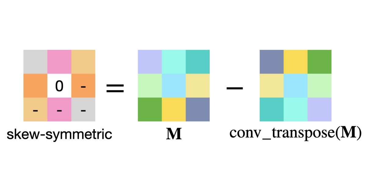
(a) Constructing a Skew-Symmetric convolution filter

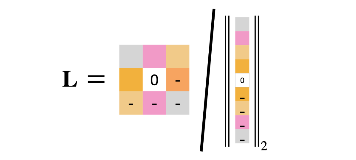
(b) Spectral normalization

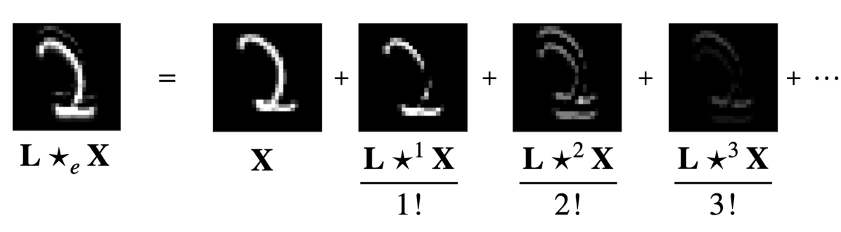
(c) Convolution exponential $(\mathbf{L}\star_{e}\mathbf{X})$

Figure 1: Each color denotes a scalar, the minus sign $(-)$ on top of some color denotes the negative of the scalar with that color. Given any convolution filter $\mathbf{M}$, we can construct a Skew-Symmetric filter (Figure 1(a)). Next, we apply spectral normalization to bound the norm of the Jacobian (Figure 1(b)). On input $\mathbf{X}$, applying convolution exponential $(\mathbf{L}\star_{e}\mathbf{X})$ results in an Orthogonal convolution (Figure 1(c)).

Li et al. (2019b) introduced an Orthogonal convolution layer called Block Convolutional Orthogonal Parametrization (BCOP). BCOP uses a clever application of $\mathrm{1D}$ Orthogonal convolution filters of sizes $2\times 1$ and $1\times 2$ to construct a $\mathrm{2D}$ Orthogonal convolution filter. It overcomes common issues of Lipschitz-constrained networks such as gradient norm attenuation and loose lipschitz bounds and enables training of large, provably 1-Lipschitz Convolutional Neural Networks (CNNs) achieving results competitive with existing methods for provable adversarial robustness. However, BCOP suffers from slow training, significant reduction in accuracy and provides no guarantees on its approximation of an Orthogonal Jacobian matrix (details in Section 2).

To address these shortcomings, we introduce an Orthogonal convolution layer called Skew Orthogonal Convolution (SOC). For provably Lipschitz CNNs, SOC results in significantly improved standard and certified robust accuracies compared to BCOP while requiring significantly less training time (Table 2). We also derive provable guarantees on our approximation of an Orthogonal Jacobian.

Our work is based on the following key mathematical property: If $\mathbf{A}$ is a Skew-Symmetric matrix (i.e. $\mathbf{A}=-\mathbf{A}^{T}$), $\exp(\mathbf{A})$ is an Orthogonal matrix (i.e. $\exp(\mathbf{A})^{T}\exp(\mathbf{A})=\exp(\mathbf{A})\exp(\mathbf{A})^{T}=\mathbf{I}$) where

$$\exp(\mathbf{A})=\mathbf{I}+\frac{\mathbf{A}}{1!}+\frac{\mathbf{A}^{2}}{2!}+\frac{\mathbf{A}^{3}}{3!}\cdots\ =\ \sum_{i=0}^{\infty}\frac{\mathbf{A}^{i}}{i!}.\quad$$ (1)

To design an Orthogonal convolution layer using this property, we need to: (a) construct Skew-Symmetric filters, i.e. convolution filters whose Jacobian is Skew-Symmetric; and (b) efficiently approximate $\exp(\mathbf{J})$ with a guaranteed small error where $\mathbf{J}$ is the Jacobian of a Skew-Symmetric filter.

To construct Skew-Symmetric convolution filters, we prove (in Theorem 2) that every Skew-Symmetric filter $\mathbf{L}$ can be written as $\mathbf{L}=\mathbf{M}-\mathrm{conv\_transpose}(\mathbf{M})$ for some filter $\mathbf{M}$ where $\mathrm{conv\_transpose}$ represents the convolution transpose operator defined in equation (3) (note that this operator is different from the matrix transpose). This result is analogous to the property that every real Skew-Symmetric matrix $\mathbf{A}$ can be written as $\mathbf{A}=\mathbf{B}-\mathbf{B}^{T}$ for some real matrix $\mathbf{B}$.

We can efficiently approximate $\exp(\mathbf{J})$ using a finite number of terms in equation (1) and the convolution exponential (Hoogeboom et al., 2020). But it is unclear whether the series can be approximated with high precision and how many terms need to be computed to achieve the desired approximation error. To resolve these issues, we derive a bound on the $l_{2}$ norm of the difference between $\exp(\mathbf{J})$ and its approximation using the first $k$ terms in equation (1), called $\mathbf{S}_{k}(\mathbf{J})$ when $\mathbf{J}$ is Skew-Symmetric (Theorem 3):

$$\|\exp(\mathbf{J})-\mathbf{S}_{k}(\mathbf{J})\|_{2}\leq\frac{\|\mathbf{J}\|_{2}^{k}}{k!}.$$ (2)

This guarantee suggests that when $\|\mathbf{J}\|_{2}$ is small, $\exp(\mathbf{J})$ can be approximated with high precision using a small number of terms. Also, the factorial term in denominator causes the error to decay very fast as $k$ increases. In our experiments, we observe that using $k=12,\ \|\mathbf{J}\|_{2}\leq 1.8$ leads to an error bound of $2.415\times 10^{-6}$. We can use spectral normalization (Miyato et al., 2018) to ensure $\|\mathbf{J}\|_{2}$ is provably bounded using the theoretical result of Singla & Feizi (2021). The design of SOC is summarized in Figure 1. Code is available at https://github.com/singlasahil14/SOC.

To summarize, we make the following contributions:

• We introduce an Orthogonal convolution layer (called Skew Orthogonal Convolution or SOC) by first designing a Skew-Symmetric convolution filter (Theorem 2) and then computing the exponential function of its Jacobian using a finite number of terms in its Taylor series.

• For a Skew-Symmetric filter with Jacobian $\mathbf{J}$, we derive a bound on the approximation error between $\exp\left(\mathbf{J}\right)$ and its $k$-term approximation (Theorem 3).

• SOC achieves significantly higher standard and provable robust accuracy on 1-Lipschitz convolutional neural networks than BCOP while requiring less training time (Table 2.) For example, SOC achieves $2.82\%$ higher standard and $3.91\%$ higher provable robust accuracy with $54.6\%$ less training time on CIFAR-10 using the LipConvnet-20 architecture (details in Section 6.5). For deeper networks ($\geq 30$ layers), SOC outperforms BCOP with an improvement of $\geq 10\%$ on both standard and robust accuracy again achieving $\geq 50\%$ reduction in the training time.

• In Theorem 4, we prove that for every Skew-Symmetric filter with Jacobian $\mathbf{J}$, there exists Skew-Symmetric matrix $\mathbf{B}$ satisfying: $\exp(\mathbf{B})=\exp(\mathbf{J}),\ \|\mathbf{B}\|_{2}\leq\pi$ . Since $\|\mathbf{J}\|_{2}$ can be large, this can allow us to reduce the approximation error without sacrificing the expressive power.

2 Related work

Provably lipschitz convolutional neural networks: Anil et al. (2018) proposed a class of fully connected neural networks (FCNs) which are Gradient Norm Preserving (GNP) and provably 1-Lipschitz using the GroupSort activation and Orthogonal weight matrices. Since then, there have been numerous attempts to tightly enforce 1-Lipschitz constraints on convolutional neural networks (CNNs) (Cissé et al., 2017; Tsuzuku et al., 2018; Qian & Wegman, 2019; Gouk et al., 2020; Sedghi et al., 2019). However, these approaches either enforce loose lipschitz bounds or are computationally intractable for large networks. Li et al. (2019b) introduced an Orthogonal convolution layer called Block Convolutional Orthogonal Parametrization (BCOP) that avoids the aforementioned issues and allows the training of large, provably 1-Lipschitz CNNs while achieving provable robust accuracy comparable with the existing methods. However, it suffers from some issues: (a) it can only represent a subset of all Orthogonal convolutions, (b) it requires a BCOP convolution filter with $2n$ channels to represent all the connected components of a BCOP convolution filter with $n$ channels thus requiring 4 times more parameters, (c) to construct a convolution filter with size $k\times k$ and $n$ input/output channels, it requires $2k-1$ matrices of size $2n\times 2n$ that must remain Orthogonal throughout training; resulting in well known difficulties of optimization over the Stiefel manifold (Edelman et al., 1998), (d) it constructs convolution filters from symmetric projectors and error in these projectors can lead to an error in the final convolution filter whereas BCOP does not provide guarantees on the error.

Provable defenses against adversarial examples: A classifier is said to be provably robust if one can guarantee that a classifier’s prediction remains constant within some region around the input. Most of the existing methods for provable robustness either bound the Lipschitz constant of the neural network or the individual layers (Weng et al., 2018; Zhang et al., 2019, 2018; Wong et al., 2018; Wong & Kolter, 2018; Raghunathan et al., 2018; Croce et al., 2019; Singh et al., 2018; Singla & Feizi, 2020). However, these methods do not scale to large and practical networks on ImageNet. To scale to such large networks, randomized smoothing (Liu et al., 2018; Cao & Gong, 2017; Lécuyer et al., 2018; Li et al., 2019a; Cohen et al., 2019; Salman et al., 2019; Kumar et al., 2020; Levine et al., 2019) has been proposed as a probabilistically certified defense. In contrast, the defense we propose in this work is deterministic and hence not directly comparable to randomized smoothing.

3 Notation

For a vector $\mathbf{v}$, $\mathbf{v}_{j}$ denotes its $j^{th}$ element. For a matrix $\mathbf{A}$, $\mathbf{A}_{j,:}$ and $\mathbf{A}_{:,k}$ denote the $j^{th}$ row and $k^{th}$ column respectively. Both $\mathbf{A}_{j,:}$ and $\mathbf{A}_{:,k}$ are assumed to be column vectors (thus $\mathbf{A}_{j,:}$ is the transpose of $j^{th}$ row of $\mathbf{A}$). $\mathbf{A}_{j,k}$ denotes the element in $j^{th}$ row and $k^{th}$ column of $\mathbf{A}$. $\mathbf{A}_{:j,:k}$ denotes the matrix containing the first $j$ rows and $k$ columns of $\mathbf{A}$. The same rules are directly extended to higher order tensors. Bold zero (i.e. $\mathbf{0}$) denotes the matrix (or tensor) consisting of zero at all elements and $\mathbf{I}$ denotes the identity matrix. $\otimes$ denotes the kronecker product. We use $\mathbb{C}$ to denote the field of complex numbers and $\mathbb{R}$ for real numbers. For a scalar $a\in\mathbb{C}$, $\overline{a}$ denotes its complex conjugate. For a matrix (or tensor) $\mathbf{A}$, $\overline{\mathbf{A}}$ denotes the element-wise complex conjugate. For $\mathbf{A}\in\mathbb{C}^{m\times n}$, $\mathbf{A}^{H}$ denotes the Hermitian transpose (i.e. $\mathbf{A}^{H}=\overline{\mathbf{A}^{T}}$). For $a\in\mathbb{C}$, $\operatorname{Re}(a)$, $\operatorname{Im}(a)$ and $|a|$ denote the real part, imaginary part and modulus of $a$, respectively. We use $\iota$ to denote the imaginary part iota (i.e. $\iota^{2}=-1$).

For a matrix $\mathbf{A}\in\mathbb{C}^{q\times r}$ and a tensor $\mathbf{B}\in\mathbb{C}^{p\times q\times r}$, $\overrightarrow{\mathbf{A}}$ denotes the vector constructed by stacking the rows of $\mathbf{A}$ and $\overrightarrow{\mathbf{B}}$ by stacking the vectors $\overrightarrow{\mathbf{B}_{j,:,:}},\ j\in[p-1]$ so that:

$$\left(\overrightarrow{\mathbf{A}}\right)^{T}=\begin{bmatrix}\mathbf{A}_{0,:}^{T}\ ,\ \mathbf{A}_{1,:}^{T}\ ,\ \ldots\ ,\ \mathbf{A}_{q-1,:}^{T}\end{bmatrix}$$

$$\left(\overrightarrow{\mathbf{B}}\right)^{T}=\begin{bmatrix}\left(\overrightarrow{\mathbf{B}_{0,:,:}}\right)^{T}\ ,\ \left(\overrightarrow{\mathbf{B}_{1,:,:}}\right)^{T}\ ,\ \ldots\ ,\ \left(\overrightarrow{\mathbf{B}_{p-1,:,:}}\right)^{T}\end{bmatrix}$$

For a $2$D convolution filter, $\mathbf{L}\in\mathbb{C}^{p\times q\times r\times s}$, we define the tensor $\mathrm{conv\_transpose}(\mathbf{L})\in\mathbb{C}^{q\times p\times r\times s}$ as follows:

$$[\mathrm{conv\_transpose}(\mathbf{L})]_{i,j,k,l}=\overline{[\mathbf{L}]}_{j,i,r-1-k,s-1-l}$$ (3)

Note that this is very different from the usual matrix transpose. See an example in Section 4. Given an input $\mathbf{X}\in\mathbb{C}^{q\times n\times n}$, we use $\mathbf{L}\star\mathbf{X}\in\mathbb{C}^{p\times n\times n}$ to denote the convolution of filter $\mathbf{L}$ with $\mathbf{X}$. We use the the notation $\mathbf{L}\star^{i}\mathbf{X}\triangleq\mathbf{L}\star^{i-1}\left(\mathbf{L}\star\mathbf{X}\right)$. Unless specified, we assume zero padding and stride 1 in each direction.

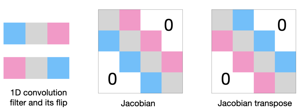
Figure 2: Each color denotes a scalar. Flipping a conv. filter (of odd size) transposes its Jacobian. Thus, any odd-sized filter that equals the negative of its flip leads to a Skew-Symmetric Jacobian.

4 Filters with Skew Symmetric Jacobians

We know that for any matrix $\mathbf{A}$ that is Skew-Symmetric ($\mathbf{A}=-\mathbf{A}^{T}$), $\exp(\mathbf{A})$ is an Orthogonal matrix:

$$\exp(\mathbf{A})\left(\exp(\mathbf{A})\right)^{T}=\left(\exp(\mathbf{A})\right)^{T}\exp(\mathbf{A})=\mathbf{I}$$

This suggests that if we can parametrize the complete set of convolution filters with Skew-Symmetric Jacobians, we can use the convolution exponential (Hoogeboom et al., 2020) to approximate an Orthogonal matrix. To construct this set, we first prove that, if convolution using filter $\mathbf{L}\in\mathbb{R}^{m\times m\times p\times q}$ ($p$ and $q$ are odd) has Jacobian $\mathbf{J}$, the convolution using $\mathrm{conv\_transpose}(\mathbf{L})$ results in Jacobian $\mathbf{J}^{T}$.

To motivate our proof, consider a filter $\mathbf{L}\in\mathbb{R}^{1\times 1\times 3\times 3}$. Applying $\mathrm{conv\_transpose}$ (equation (3)), we get:

$$\mathbf{L}=\begin{bmatrix}a&b&c\\ d&e&f\\ g&h&i\end{bmatrix},\quad\mathrm{conv\_transpose}\left(\mathbf{L}\right)=\begin{bmatrix}i&h&g\\ f&e&d\\ c&b&a\end{bmatrix}$$

That is, for a $\mathrm{2D}$ convolution filter with 1 channel, $\mathrm{conv\_transpose}$ flips it along the horizontal and vertical directions. To understand why this flipping transposes the Jacobian, we provide another example for a $\mathrm{1D}$ convolution filter in Figure 2. Our proof uses the following expression for the Jacobian of convolution using a filter $\mathbf{L}\in\mathbb{R}^{1\times 1\times(2p+1)\times(2q+1)}$ and input $\mathbf{X}\in\mathbb{R}^{1\times n\times n}$:

$$\mathbf{J}=\sum_{i=-p}^{p}\sum_{j=-q}^{q}\mathbf{L}_{0,0,p+i,q+j}\left(\mathbf{P}^{(i)}\otimes\mathbf{P}^{(j)}\right)$$

where $\mathbf{P}^{(k)}\in\mathbb{R}^{n\times n}$, $\mathbf{P}^{(k)}_{i,j}=1$ if $i-j=k$ and $0$ otherwise. The above equation leads to the following theorem:

Theorem 1.

Consider a $\mathrm{2D}$ convolution filter $\mathbf{L}\in\mathbb{R}^{m\times m\times(2p+1)\times(2q+1)}$ and input $\mathbf{X}\in\mathbb{R}^{m\times n\times n}$. Let $\mathbf{J}=\nabla_{\overrightarrow{\mathbf{X}}}\ \overrightarrow{\left(\mathbf{L}\star\mathbf{X}\right)}$, then $\mathbf{J}^{T}=\nabla_{\overrightarrow{\mathbf{X}}}\ \overrightarrow{\left(\mathrm{conv\_transpose}(\mathbf{L})\star\mathbf{X}\right)}$.

Next, we prove that any $\mathrm{2D}$ convolution filter $\mathbf{L}$ whose Jacobian is a Skew-Symmetric matrix can be expressed as: $\mathbf{L}=\mathbf{M}-\mathrm{conv\_transpose}(\mathbf{M})$ where $\mathbf{M}$ has the same dimensions as $\mathbf{L}$. This allows us to parametrize the set of all convolution filters with Skew-Symmetric Jacobian matrices.

Theorem 2.

Consider a $\mathrm{2D}$ convolution filter $\mathbf{L}\in\mathbb{R}^{m\times m\times(2p+1)\times(2q+1)}$ and input $\mathbf{X}\in\mathbb{R}^{m\times n\times n}$. The Jacobian $\nabla_{\overrightarrow{\mathbf{X}}}\ \overrightarrow{\left(\mathbf{L}\star\mathbf{X}\right)}$ is Skew-Symmetric if and only if:

$$\mathbf{L}=\mathbf{M}-\mathrm{conv\_transpose}(\mathbf{M})$$

for some filter $\mathbf{M}\in\mathbb{R}^{m\times m\times(2p+1)\times(2q+1)}$.

We prove Theorems 1 and 2 for the more general case of complex convolution filters ($\mathbf{L}_{i,j,k,l}\in\mathbb{C}$) in Appendix Sections B.1 and B.2. Theorem 2 allow us to convert any arbitrary convolution filter into a filter with a Skew-Symmetric Jacobian. This leads to the following definition:

Definition 1.

(Skew-Symmetric Convolution Filter) A convolution filter $\mathbf{L}\in\mathbb{R}^{m\times m\times(2p+1)\times(2q+1)}$ is said to be Skew-Symmetric if given an input $\mathbf{X}\in\mathbb{R}^{m\times n\times n}$, the Jacobian matrix $\nabla_{\overrightarrow{\mathbf{X}}}\ \overrightarrow{\left(\mathbf{L}\star\mathbf{X}\right)}$ is Skew-Symmetric.

We note that although Theorem 2 requires the height and width of $\mathbf{M}$ to be odd integers, we can also construct a Skew-Symmetric filter when $\mathbf{M}$ has even height/width by zero padding $\mathbf{M}$ to make the desired dimensions odd.

5 Skew Orthogonal Convolution layers

In this section, we derive a method to approximate the exponential of the Jacobian of a Skew-Symmetric convolution filter (i.e. $\exp(\mathbf{J})$). We also derive a bound on the approximation error. Given an input $\mathbf{X}\in\mathbb{R}^{m\times n\times n}$ and a Skew-Symmetric convolution filter $\mathbf{L}\in\mathbb{R}^{m\times m\times k\times k}$ ($k$ is odd), let $\mathbf{J}$ be the Jacobian of convolution filter $\mathbf{L}$ so that:

$$\mathbf{J}\overrightarrow{\mathbf{X}}=\overrightarrow{\left(\mathbf{L}\star\mathbf{X}\right)}$$ (4)

By construction, we know that $\mathbf{J}$ is a Skew-Symmetric matrix, thus $\exp(\mathbf{J})$ is an Orthogonal matrix. We are interested in computing $\exp\left(\mathbf{J}\right)\overrightarrow{\mathbf{X}}$ efficiently where:

$$\exp\left(\mathbf{J}\right)\overrightarrow{\mathbf{X}}=\overrightarrow{\mathbf{X}}+\frac{\mathbf{J}\overrightarrow{\mathbf{X}}}{1!}+\frac{\mathbf{J}^{2}\overrightarrow{\mathbf{X}}}{2!}+\frac{\mathbf{J}^{3}\overrightarrow{\mathbf{X}}}{3!}+\cdots$$

Using equation (4), the above expression can be written as:

$$\exp\left(\mathbf{J}\right)\overrightarrow{\mathbf{X}}=\overrightarrow{\mathbf{X}}+\overrightarrow{\frac{\mathbf{L}\star\mathbf{X}}{1!}}+\overrightarrow{\frac{\mathbf{L}\star^{2}\mathbf{X}}{2!}}+\overrightarrow{\frac{\mathbf{L}\star^{3}\mathbf{X}}{3!}}+\cdots$$

where the notation $\mathbf{L}\star^{i}\mathbf{X}\triangleq\mathbf{L}\star^{i-1}(\mathbf{L}\star\mathbf{X})$. Using the above equation, we define $\mathbf{L}\star_{e}\mathbf{X}$ as follows:

$$\mathbf{L}\star_{e}\mathbf{X}=\mathbf{X}+\frac{\mathbf{L}\star\mathbf{X}}{1!}+\frac{\mathbf{L}\star^{2}\mathbf{X}}{2!}+\frac{\mathbf{L}\star^{3}\mathbf{X}}{3!}+\cdots$$ (5)

The above operation is called convolution exponential, and was introduced by Hoogeboom et al. (2020). By construction, $\mathbf{L}\star_{e}\mathbf{X}$ satisfies: $\exp\left(\mathbf{J}\right)\overrightarrow{\mathbf{X}}=\overrightarrow{\mathbf{L}\star_{e}\mathbf{X}}$. Thus, the Jacobian of $\overrightarrow{\mathbf{L}\star_{e}\mathbf{X}}$ with respect to $\overrightarrow{\mathbf{X}}$ is equal to $\exp(\mathbf{J})$ which is Orthogonal (since $\mathbf{J}$ is Skew-Symmetric). However, $\mathbf{L}\star_{e}\mathbf{X}$ can only be approximated using a finite number of terms in the series given in equation (5). Thus, we need to bound the error of such an approximation.

5.1 Bounding the Approximation Error

To bound the approximation error using a finite number of terms, first note that since the Jacobian matrix $\mathbf{J}$ is Skew-Symmetric, all the eigenvalues are purely imaginary. For a purely imaginary scalar $\lambda\in\mathbb{C}$ (i.e. $\operatorname{Re}(\lambda)=0$), we first bound the error between $\exp(\lambda)$ and approximation $p_{k}(\lambda)$ computed using $k$ terms of the exponential series as follows:

$$\big{|}\exp(\lambda)-p_{k}(\lambda)\big{|}\leq\frac{|\lambda|^{k}}{k!},\qquad\forall\ \lambda:\operatorname{Re}(\lambda)=0$$ (6)

The above result then allows us to prove the following result for a Skew-Symmetric matrix in a straightforward manner:

Theorem 3.

For Skew-Symmetric $\mathbf{J}$, we have the inequality:

$$\|\exp(\mathbf{J})-\mathbf{S}_{k}(\mathbf{J})\|_{2}\leq\frac{\|\mathbf{J}\|_{2}^{k}}{k!}\ \ \ \text{where}\ \mathbf{S}_{k}(\mathbf{J})=\sum_{i=0}^{k-1}\frac{\mathbf{J}^{i}}{i!}\quad$$

A more general proof of Theorem 3 (for $\mathbf{J}\in\mathbb{C}^{n\times n}$ and skew-Hermitian i.e. $\mathbf{J}=-\mathbf{J}^{H}$) is given in Appendix Section B.3. The above theorem allows us to bound the approximation error between the true matrix exponential (which is Orthogonal) and its $k$ term approximation as a function of the number of terms ($k$) and the Jacobian norm $\|\mathbf{J}\|_{2}$. The factorial term in the denominator causes the error to decay very fast as the number of terms increases. We call the resulting algorithm Skew Orthogonal Convolution (SOC).

We emphasize that the above theorem is valid only for Skew-Symmetric matrices and hence not directly applicable for the convolution exponential (Hoogeboom et al., 2020).

Input: feature map: $\mathbf{X}\in\mathbb{R}^{c_{i}\times n\times n}$, convolution filter: $\mathbf{M}\in\mathbb{R}^{m\times m\times h\times w}$ $\left(m=\max(c_{i},\ c_{o})\right)$ , terms: $K$

Output: output after applying convolution exponential: $\mathbf{Y}$

if $c_{i}<c_{o}$ then

       $\mathbf{X}^{\prime}\leftarrow\mathrm{pad}(\mathbf{X},\ (c_{o}-c_{i},0,0))$

end if

$\mathbf{L}\leftarrow\mathbf{M}-\mathrm{conv\_transpose}(\mathbf{M})$
$\mathbf{L}\leftarrow\mathrm{spectral\_normalization}(\mathbf{L})$
$\mathbf{Y}\leftarrow\mathbf{X}^{\prime}$
$\mathrm{factorial}\leftarrow 1$
for $j\leftarrow 2$ to $K$ do

       $\mathbf{X}^{\prime}\leftarrow\mathbf{L}\star\mathbf{X}^{\prime}$
$\mathrm{factorial}\leftarrow\mathrm{factorial}*(j-1)$
$\mathbf{Y}\to\mathbf{Y}+\left(\mathbf{X}^{\prime}/\mathrm{factorial}\right)$

end for

if $c_{i}>c_{o}$ then

       $\mathbf{Y}\leftarrow\mathbf{Y}[0:c_{o},\ :\ ,\ :\ ]$

end if

Return: $\mathbf{Y}$

Algorithm 1 Skew Orthogonal Convolution

5.2 Complete Set of Skew Orthogonal Convolutions

Observe that for $\operatorname{Re}(\lambda)=0$, (i.e. $\lambda=\iota\theta,\ \theta\in\mathbb{R}$), we have:

$$\ \ \ \exp(\lambda)=\exp(\lambda+2\iota\pi k)=\cos(\theta)+\iota\sin(\theta),\ \ k\in\mathbb{Z}$$

This suggests that we can shift $\lambda$ by integer multiples of $2\pi\iota$ without changing $\exp(\lambda)$ while reducing the approximation error (using Theorem 3). For example, $\exp(\iota\pi/3)$ requires fewer terms to achieve the desired approximation (using equation (6)) than say $\exp(\iota(\pi/3+2\pi))$ because the latter has higher norm (i.e. $2\pi+\pi/3=7\pi/3$) than the former (i.e. $\pi/3$). This insight leads to the following theorem:

Theorem 4.

Given a real Skew-Symmetric matrix $\mathbf{A}$, we can construct another real Skew-Symmetric matrix $\mathbf{B}$ such that $\mathbf{B}$ satisfies: (i) $\exp(\mathbf{A})=\exp(\mathbf{B})$ and (ii) $\|\mathbf{B}\|_{2}\leq\pi$.

A proof is given in Appendix Section B.4. This proves that every real Skew-Symmetric Jacobian matrix $\mathbf{J}$ (associated with some Skew-Symmetric convolution filter $\mathbf{L}$) can be replaced with a Skew-Symmetric Jacobian $\mathbf{B}$ such that $\exp\left(\mathbf{B}\right)=\exp\left(\mathbf{J}\right)$ and $\|\mathbf{B}\|_{2}\leq\pi$ (note that $\|\mathbf{J}\|_{2}$ can be arbitrarily large). This strictly reduces the approximation error (Theorem 3) without sacrificing the expressive power.

We make the following observations about Theorem 4: (a) If $\mathbf{J}$ is equal to the Jacobian of some Skew-Symmetric convolution filter, $\mathbf{B}$ may not satisfy this property, i.e. it may not exhibit the block doubly toeplitz structure of the Jacobian of a $\mathrm{2D}$ convolution filter (Sedghi et al., 2019) and thus may not equal the jacobian of some Skew-Symmetric convolution filter; (b) even if $\mathbf{B}$ satisfies this property, the filter size of the Skew-Symmetric filter whose Jacobian equals $\mathbf{B}$ can be very different from that of the filter with Jacobian $\mathbf{J}$.

In this sense, Theorem 4 cannot directly be used to parametrize the complete set of SOC  because it is not clear how to efficiently parametrize the set of all matrices $\mathbf{B}$ that satisfy (a) $\|\mathbf{B}\|_{2}\leq\pi$ and (b) $\exp(\mathbf{B})=\exp(\mathbf{J})$ where $\mathbf{J}$ is the Jacobian of some Skew-Symmetric convolution filter. We leave this question of efficient parametrization of Skew Orthogonal Convolution layers open for future research.

5.3 Extensions to $\mathrm{3D}$ and Complex Convolutions

When the matrix $\mathbf{A}\in\mathbb{C}^{n\times n}$ is skew-Hermitian ($\mathbf{A}=-\mathbf{A}^{H}$), then $\exp(\mathbf{A})$ is a unitary matrix:

$$\exp(\mathbf{A})\left(\exp(\mathbf{A})\right)^{H}=\left(\exp(\mathbf{A})\right)^{H}\exp(\mathbf{A})=\mathbf{I}$$

To use the above property to construct a unitary convolution layer with complex weights, we first define:

Definition 2.

(Skew-Hermitian Convolution Filter) A convolution filter $\mathbf{L}\in\mathbb{C}^{m\times m\times(2p+1)\times(2q+1)}$ is said to be Skew-Hermitian if given an input $\mathbf{X}\in\mathbb{C}^{m\times n\times n}$, the Jacobian matrix $\nabla_{\overrightarrow{\mathbf{X}}}\ \overrightarrow{\left(\mathbf{L}\star\mathbf{X}\right)}$ is Skew-Hermitian.

Using the extensions of Theorems 1 and 2 for complex convolution filters (proofs in Appendix Sections B.1 and B.2), we can construct a $\mathrm{2D}$ Skew-Hermitian convolution filter. Next, using an extension of Theorem 3 for complex Skew-Hermitian matrices (proof in Appendix Section B.3), we can get exactly the same bound on the approximation error. The resulting algorithm is called Skew Unitary Convolution  (SUC). We also prove an extension of Theorem 4 for complex Skew-Hermitian matrices in Appendix Section B.5. We discuss the construction of $\mathrm{3D}$ Skew-Hermitian convolution filters in Appendix Sections B.6 and B.7.

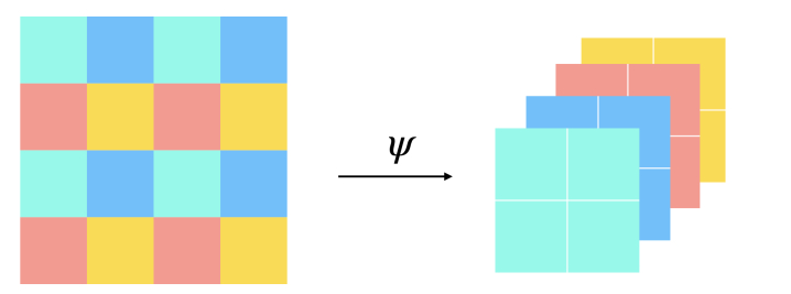
Figure 3: Invertible downsampling operation $\psi$

6 Implementation details of SOC

In this section, we explain the key implementation details of SOC (summarized in Algorithm 1).

6.1 Bounding the norm of Jacobian

To bound the norm of the Jacobian of Skew-Symmetric convolution filter, we use the following result:

Theorem.

(Singla & Feizi, 2021) Consider a convolution filter $\mathbf{L}\in\mathbb{R}^{c_{o}\times c_{i}\times h\times w}$ applied to input $\mathbf{X}$. Let $\mathbf{J}$ be the Jacobian of $\mathbf{L}\star\mathbf{X}$ w.r.t $\mathbf{X}$, we have the following inequality:

$$\|\mathbf{J}\|_{2}\leq\sqrt{hw}\ \min\left(\|\mathbf{R}\|_{2},\|\mathbf{S}\|_{2},\|\mathbf{T}\|_{2},\|\mathbf{U}\|_{2}\right),$$

where $\mathbf{R}\in\mathbb{R}^{c_{o}h\times c_{i}w},\mathbf{S}\in\mathbb{R}^{c_{o}w\times c_{i}h},\mathbf{T}\in\mathbb{R}^{c_{o}\times c_{i}hw}$ and $\mathbf{U}\in\mathbb{R}^{c_{o}hw\times c_{i}}$ are obtained by reshaping the filter $\mathbf{L}$.

Using the above theorem, we divide the Skew-Symmetric convolution filter by $\min\left(\|\mathbf{R}\|_{2},\|\mathbf{S}\|_{2},\|\mathbf{T}\|_{2},\|\mathbf{U}\|_{2}\right)$ so that the spectral norm of the resulting filter is bounded by $\sqrt{hw}$. We next multiply the normalized filter with the hyperparameter, $0.7$ as we find that it allows faster convergence with no loss in performance. Unless specified, we use $h=w=3$ in all of our experiments resulting in the norm bound of $2.1$. Note that while the above theorem also allows us to bound the Lipschitz constant of a convolution layer, for deep networks (say $40$ layers), the Lipschitz bound (assuming a $1$-Lipschitz activation function) would increase to $2.1^{40}=7.74\times 10^{12}$. Thus, the above bound alone is unlikely to enforce a tight global Lipschitz constraint.

6.2 Different input and output channels

In general, we may want to construct an orthogonal convolution that maps from $c_{i}$ input channels to $c_{o}$ output channels where $c_{i}\neq c_{o}$. Consider the two cases:

Case 1 ($c_{o}<c_{i}$): We construct a Skew-Symmetric convolution filter with $c_{i}$ channels. After applying the exponential, we select the first $c_{o}$ output channels from the output layer.

Case 2 ($c_{o}>c_{i}$): We use a Skew-Symmetric convolution filter with $c_{o}$ channels. We zero pad the input with $c_{o}-c_{i}$ channels and then compute the convolution exponential.

6.3 Strided convolution

Given an input $\mathbf{X}\in\mathbb{R}^{c_{i}\times n\times n}$ ($n$ is even), we may want to construct an orthogonal convolution with output $\mathbf{Y}\in\mathbb{R}^{c_{o}\times(n/2)\times(n/2)}$ (i.e. an orthogonal convolution with stride $2$). To perform a strided convolution, we first apply invertible downsampling $\psi$ as shown in Figure 3 (Jacobsen et al., 2018) to construct $\mathbf{X}^{\prime}\in\mathbb{R}^{4c_{i}\times(n/2)\times(n/2)}$. Next, we apply convolution exponential to $\mathbf{X}^{\prime}$ using a Skew-Symmetric convolution filter with $4c_{i}$ input and $c_{o}$ output channels.

6.4 Number of terms for the approximation

During training, we use $6$ terms to approximate the exponential function for speed. During evaluation, we use $12$ terms to ensure that the exponential of the Jacobian is sufficiently close to being an orthogonal matrix.

Output Size	Convolution layer	Repeats
$16\times 16$	conv $[3\times 3,32,1]$	$(n/5)-1$
	conv $[3\times 3,64,2]$	1
$8\times 8$	conv $[3\times 3,64,1]$	$(n/5)-1$
	conv $[3\times 3,128,2]$	1
$4\times 4$	conv $[3\times 3,128,1]$	$(n/5)-1$
	conv $[3\times 3,256,2]$	1
$2\times 2$	conv $[3\times 3,256,1]$	$(n/5)-1$
	conv $[3\times 3,512,2]$	1
$1\times 1$	conv $[3\times 3,512,1]$	$(n/5)-1$
	conv $[1\times 1,1024,2]$	1

Table 1: LipConvnet-n Architecture. Each convolution layer is followed by the $\mathrm{MaxMin}$ activation.

6.5 Network architecture

We design a provably 1-Lipschitz architecture called LipConvnet-$n$ ($n$ is the number of convolution layers and a multiple of $5$ in our experiments). It consists of $(n/5)-1$ Orthogonal convolutions of stride 1 (followed by the $\mathrm{MaxMin}$ activation function), followed by Orthogonal convolution of stride 2 (again followed by the $\mathrm{MaxMin}$). It is summarized in Table 1. conv $[k\times k,m,s]$ denotes convolution layer with filter of size $k\times k$, out channels $m$ and stride $s$. It is followed by a fully connected layer to output the class logits. The $\mathrm{MaxMin}$ activation function (Anil et al., 2018) is described in Appendix Section C.

Model	Conv. Type	CIFAR-10			CIFAR-100
		Standard Accuracy	Robust Accuracy	Time per epoch (s)	Standard Accuracy	Robust Accuracy	Time per epoch (s)
LipConvnet-5	BCOP	74.35%	58.01%	96.153	42.61%	28.67%	94.463
	SOC	75.78%	59.16%	31.096	42.73%	27.82%	30.844
LipConvnet-10	BCOP	74.47%	58.48%	122.115	42.08%	27.75%	119.038
	SOC	76.48%	60.82%	48.242	43.71%	29.39%	48.363
LipConvnet-15	BCOP	73.86%	57.39%	145.944	39.98%	26.17%	144.173
	SOC	76.68%	61.30%	63.742	42.93%	28.79%	63.540
LipConvnet-20	BCOP	69.84%	52.10%	170.009	36.13%	22.50%	172.266
	SOC	76.43%	61.92%	77.226	43.07%	29.18%	76.460
LipConvnet-25	BCOP	68.26%	49.92%	207.359	28.41%	16.34%	205.313
	SOC	75.19%	60.18%	98.534	43.31%	28.59%	95.950
LipConvnet-30	BCOP	64.11%	43.39%	227.916	26.87%	14.03%	229.840
	SOC	74.47%	59.04%	110.531	42.90%	28.74%	107.163
LipConvnet-35	BCOP	63.05%	41.72%	267.272	21.71%	10.33%	274.256
	SOC	73.70%	58.44%	130.671	42.44%	28.31%	126.368
LipConvnet-40	BCOP	60.17%	38.87%	295.350	19.97%	8.66%	289.369
	SOC	71.63%	54.36%	144.556	41.83%	27.98%	140.458

Table 2: Results for provable robustness against adversarial examples ($l_{2}$ perturbation radius of 36/255). Time per epoch is the training time per epoch (in seconds).

7 Experiments

Our goal is to evaluate the expressiveness of our method (SOC) compared to BCOP for constructing Orthogonal convolutional layers. To study this, we perform experiments in three settings: (a) provably robust image classification, (b) standard training and (c) adversarial training.

All experiments were performed using $1$ NVIDIA GeForce RTX 2080 Ti GPU. All networks were trained for 200 epochs with an initial learning rate 0.1, dropped by a factor of 0.1 after 50 and 150 epochs. We use no weight decay for training with BCOP convolution as it significantly reduces its performance. For training with standard convolution and SOC, we use a weight decay of $10^{-4}$.

To evaluate the approximation error for SOC at convergence (using Theorem 3), we compute the norm of the Jacobian of the Skew-Symmetric convolution filter using real normalization (Ryu et al., 2019). We observe that the maximum norm (across different experiments and layers of the network) is below $1.8$ (i.e. slightly below the theoretical upper bound of $2.1$ discussed in Section 6.1) resulting in a maximum error of $1.8^{12}/12!=2.415\times 10^{-6}$.

7.1 Provable Defenses against Adversarial Attacks

To certify provable robustness of $1$-Lipschitz network $f$ for some input $\mathbf{x}$, we first define the margin of prediction: $\mathcal{M}_{f}(\mathbf{x})=\max\left(0,y_{t}-\max_{i\neq t}y_{i}\right)$ where $\mathbf{y}=[y_{1},y_{2,\dotsc}]$ is the predicted logits from $f$ on $\mathbf{x}$ and $y_{t}$ is the correct logit. Using Theorem 7 in Li et al. (2019b), we can derive the robustness certificate as $\mathcal{M}_{f}(\mathbf{x})/\sqrt{2}$. The provable robust accuracy, evaluated using an $l_{2}$ perturbation radius of $36/255$ (same as in Li et al. (2019b)) equals the fraction of data points ($\mathbf{x}$) in the test dataset satisfying $\mathcal{M}_{f}(\mathbf{x})/\sqrt{2}\geq 36/255$.

In Table 2, we show the results of our experiments using different LipConvnet architectures with varying number of layers on CIFAR-10 and CIFAR-100 datasets. We make the following observations: (a) SOC  achieves significantly higher standard and provable robust accuracy than BCOP for different architectures and datasets, (b) SOC requires significantly less training time per epoch than BCOP and (c) as the number of layers increases, the performance of BCOP degrades rapidly but that of SOC remains largely consistent. For example, on a LipConvnet-40 architecture, SOC achieves $11.46\%$ higher standard accuracy; $15.49\%$ higher provable robust accuracy on the CIFAR-10 dataset and $21.86\%$ higher standard accuracy; $19.32\%$ higher provable robust accuracy on the CIFAR-100 dataset. We further emphasize that none of the other well known deterministic provable defenses (discussed in Section 2) are scalable to large networks as the ones in Table 2. BCOP, while scalable, achieves significantly lower standard and provable robust accuracies for deep networks than SOC.

Model	Conv. Type	CIFAR-10		CIFAR-100
		Standard Accuracy	Time per epoch (s)	Standard Accuracy	Time per epoch (s)
Resnet-18	Standard	95.10%	13.289	77.60%	13.440
	BCOP	92.38%	128.383	71.16%	128.146
	SOC	94.24%	110.750	74.55%	103.633
Resnet-34	Standard	95.54%	22.348	78.60%	22.806
	BCOP	93.79%	237.068	73.38%	235.367
	SOC	94.44%	170.864	75.52%	164.178
Resnet-50	Standard	95.47%	38.834	78.11%	37.454
	SOC	94.68%	584.762	77.95%	597.297

Table 3: Results for standard accuracy. For Resnet-50, we observe OOM (Out Of Memory) error when using BCOP.

Model	Conv. Type	CIFAR-10			CIFAR-100
		Standard Accuracy	Robust Accuracy	Time per epoch (s)	Standard Accuracy	Robust Accuracy	Time per epoch (s)
Resnet-18	Standard	83.05%	44.39%	28.139	59.87%	22.78%	28.147
	BCOP	79.26%	34.85%	264.694	54.80%	16.00%	252.868
	SOC	82.24%	43.73%	203.860	58.95%	22.65%	199.188

Table 4: Results for empirical robustness against adversarial examples ($l_{\infty}$ perturbation radius of 8/255).

7.2 Standard Training

For standard training, we perform experiments using Resnet-18, Resnet-34 and Resnet-50 architectures on CIFAR-10 and CIFAR-100 datasets. Results are presented in Table 3. We again observe that SOC  achieves higher standard accuracy than BCOP on different architectures and datasets while requiring significantly less time to train. For Resnet-50, the performance of SOC almost matches that of standard convolution layers while BCOP results in an Out Of Memory (OOM) error. However, for Resnet-18 and Resnet-34, the difference is not as significant as the one observed for LipConvnet architectures in Table 2. We conjecture that this is because the residual connections allows the gradient to flow relatively freely compared to being restricted to flow through the convolution layers in LipConvnet architectures.

7.3 Adversarial Training

For adversarial training, we use a threat model with an $l_{\infty}$ attack radius of $8/255$. Note that we use the $l_{\infty}$ threat model (instead of $l_{2}$) because it is known to be a stronger adversarial threat model for evaluating empirical robustness (Madry et al., 2018). For training, we use the FGSM variant by Wong et al. (2020). For evaluation, we use 50 iterations of PGD with step size of $2/255$ and 10 random restarts. Results are presented in Table 4. We observe that for Resnet-18 architecture and on both CIFAR-10 and CIFAR-100 datasets, SOC results in significantly improved standard and empirical robust accuracy compared to BCOP while requiring significantly less time to train. The performance of SOC comes close to the performance of a standard convolution layer with the difference being less than $1\%$ for both standard and robust accuracy on both the datasets.

8 Discussion and Future work

In this work, we design a new orthogonal convolution layer by first constructing a Skew-Symmetric convolution filter and then applying the convolution exponential (Hoogeboom et al., 2020) to the filter. We also derive provable guarantees on the approximation of the exponential using a finite number of terms. Our method achieves significantly higher accuracy than BCOP for various network architectures and datasets under standard, adversarial and provably robust training setups while requiring less training time per epoch. We suggest the following directions for future research:

Reducing the evaluation time: While SOC requires less time to train than BCOP, it requires more time for evaluation because the convolution filter needs to be applied multiple times to approximate the orthogonal matrix with the desired error. In contrast, BCOP constructs an orthogonal convolution filter that needs to be applied only once during evaluation. From Theorem 3, we know that we can reduce the number of terms required to achieve the desired approximation error by reducing the Jacobian norm $\|\mathbf{J}\|_{2}$. Training approaches such as spectral norm regularization (Singla & Feizi, 2021) and singular value clipping (Sedghi et al., 2019) can be useful to further lower $\|\mathbf{J}\|_{2}$ and thus reduce the evaluation time.

Complete Set of SOC convolutions: While Theorem 4 suggests that the complete set of SOC convolutions can be constructed from a subset of Skew-Symmetric matrices $\mathbf{B}$ that satisfy (a) $\|\mathbf{B}\|_{2}\leq\pi$ and (b) $\exp(\mathbf{B})=\exp(\mathbf{A})$ where $\mathbf{A}$ is the Jacobian of some Skew-Symmetric convolution filter, it is an open question how to efficiently parametrize this subset for training Lipschitz convolutional neural networks. This remains an interesting problem for future research.

9 Acknowledgements

This project was supported in part by NSF CAREER AWARD 1942230, HR001119S0026, HR00112090132, NIST 60NANB20D134 and Simons Fellowship on ”Foundations of Deep Learning.”

Appendix

Appendix A Notation

For $n\in\mathbb{N}$, we use $[n]$ to denote the set $\{0,\dots,n\}$. For a vector $\mathbf{v}$, we use $\mathbf{v}_{j}$ to denote the element in the $j^{th}$ position of the vector. We use $\mathbf{A}_{j,:}$ and $\mathbf{A}_{:,k}$ to denote the $j^{th}$ row and $k^{th}$ column of the matrix $\mathbf{A}$ respectively. We assume both $\mathbf{A}_{j,:}$, $\mathbf{A}_{:,k}$ to be column vectors (thus $\mathbf{A}_{j,:}$ is the transpose of $j^{th}$ row of $\mathbf{A}$). $\mathbf{A}_{j,k}$ denotes the element in $j^{th}$ row and $k^{th}$ column of $\mathbf{A}$. $\mathbf{A}_{j,:k}$ and $\mathbf{A}_{:j,k}$ denote the vectors containing the first $k$ elements of the $j^{th}$ row and first $j$ elements of $k^{th}$ column, respectively. $\mathbf{A}_{:j,:k}$ denotes the matrix containing the first $j$ rows and $k$ columns of $\mathbf{A}$. The same rules can be directly extended to higher order tensors. We use bold zero i.e $\mathbf{0}$ to denote the matrix (or tensor) consisting of zero at all elements, $\mathbf{I}_{n}$ to denote the identity matrix of size $n\times n$. We use $\mathbb{C}$ to denote the field of complex numbers and $\mathbb{R}$ for real numbers. For a scalar $a\in\mathbb{C}$, $\overline{a}$ denotes its complex conjugate. For a vector $\mathbf{v}$ or matrix (or tensor) $\mathbf{A}$, $\overline{\mathbf{v}}$ or $\overline{\mathbf{A}}$ denotes the element-wise complex conjugate. For $\mathbf{A}\in\mathbb{C}^{m\times n}$, $\mathbf{A}^{H}$ denotes the hermitian transpose i.e $\mathbf{A}^{H}=\overline{\mathbf{A}^{T}}$. For a scalar $a\in\mathbb{C}$, $\operatorname{Re}(a)$, $\operatorname{Im}(a)$ and $|a|$ denote the real part, imaginary part and modulus of $a$ respectively. We use $[a,b)$ where $a,b\in\mathbb{C}$ to denote the set consisting of complex scalars on the line connecting $a$ and $b$ (including $a$, but excluding $b$). $\mathbf{A}\otimes\mathbf{B}$ denotes the kronecker product between matrices $\mathbf{A}$ and $\mathbf{B}$. We use $\iota$ to denote iota (i.e $\iota^{2}=-1$).

For a matrix $\mathbf{A}\in\mathbb{C}^{q\times r}$ and a tensor $\mathbf{B}\in\mathbb{C}^{p\times q\times r}$, $\overrightarrow{\mathbf{A}}$ denotes the vector constructed by stacking the rows of $\mathbf{A}$ and $\overrightarrow{\mathbf{B}}$ by stacking the vectors $\overrightarrow{\mathbf{B}_{j,:,:}},\ j\in[p-1]$ so that:

$$\left(\overrightarrow{\mathbf{A}}\right)^{T}=\begin{bmatrix}\mathbf{A}_{0,:}^{T}\ ,\ \mathbf{A}_{1,:}^{T}\ ,\ \ldots\ ,\ \mathbf{A}_{q-1,:}^{T}\end{bmatrix}$$

$$\left(\overrightarrow{\mathbf{B}}\right)^{T}=\begin{bmatrix}\left(\overrightarrow{\mathbf{B}_{0,:,:}}\right)^{T}\ ,\ \left(\overrightarrow{\mathbf{B}_{1,:,:}}\right)^{T}\ ,\ \ldots\ ,\ \left(\overrightarrow{\mathbf{B}_{p-1,:,:}}\right)^{T}\end{bmatrix}$$

For a $2$D convolution filter, $\mathbf{L}\in\mathbb{C}^{p\times q\times r\times s}$, we define the tensor $\mathrm{conv\_transpose}(\mathbf{L})\in\mathbb{C}^{q\times p\times r\times s}$ as follows:

$$[\mathrm{conv\_transpose}(\mathbf{L})]_{i,j,k,l}=\overline{[\mathbf{L}]}_{j,i,r-1-k,s-1-l}$$ (7)

Note that this is very different from the usual matrix transpose. Given an input $\mathbf{X}\in\mathbb{C}^{q\times n\times n}$, we use $\mathbf{L}\star\mathbf{X}\in\mathbb{C}^{p\times n\times n}$ to denote the convolution of filter $\mathbf{L}$ with $\mathbf{X}$. The notation $\mathbf{L}\star^{i}\mathbf{X}\triangleq\mathbf{L}\star^{i-1}\left(\mathbf{L}\star\mathbf{X}\right)$. Unless specified otherwise, we assume zero padding and stride 1 in each direction.

Appendix B Proofs

B.1 Proof of Theorem 1

Theorem.

Consider a convolution filter $\mathbf{L}\in\mathbb{C}^{m\times m\times(2p+1)\times(2q+1)}$ applied to an input $\mathbf{X}\in\mathbb{C}^{m\times n\times n}$ that results in output $\mathbf{Y}=\mathbf{L}\star\mathbf{X}\in\mathbb{C}^{m\times n\times n}$. Let $\mathbf{J}$ be the jacobian of $\overrightarrow{\mathbf{Y}}$ with respect to $\overrightarrow{\mathbf{X}}$ , then the jacobian for convolution with the filter $\mathrm{conv\_transpose}(\mathbf{L})$ is equal to $\mathbf{J}^{H}$.

Proof.

We first prove the above result assuming $m=1$.
Assuming $\mathbf{m=1}$:
We know that $\mathbf{J}$ is a doubly toeplitz matrix of size $n^{2}\times n^{2}$:

$$\mathbf{J}=\begin{bmatrix}\mathbf{J}^{(0)}&\mathbf{J}^{(-1)}&\cdots&\mathbf{J}^{(-p)}&0\\ \mathbf{J}^{(1)}&\mathbf{J}^{(0)}&\mathbf{J}^{(-1)}&\ddots&\ddots\\ \vdots&\mathbf{J}^{(1)}&\mathbf{J}^{(0)}&\ddots&\ddots\\ \mathbf{J}^{(p)}&\ddots&\ddots&\ddots&\mathbf{J}^{(-1)}\\ 0&\ddots&\ddots&\mathbf{J}^{(1)}&\mathbf{J}^{(0)}\end{bmatrix}$$

In the above equation, each $\mathbf{J}^{(i)}$ is a toeplitz matrix of size $n\times n$. Define $\mathbf{P}^{(k)}$ as a $n\times n$ matrix with $\mathbf{P}^{(k)}_{i,j}=1$ if $i-j=k$ and $0$ otherwise. Thus $\mathbf{J}$ can be written as:

$$\mathbf{J}=\sum_{i=-p}^{p}\mathbf{P}^{(i)}\otimes\mathbf{J}^{(i)}$$

Since each matrix $\mathbf{J}^{(i)}$ is a toeplitz matrix, it can be written as follows. Because the first two dimensions of filter $\mathbf{L}$ are of size $1$, we index $\mathbf{L}$ using only the last two indices:

$$\mathbf{J}^{(i)}=\sum_{j=-q}^{q}\mathbf{L}_{p+i,q+j}\mathbf{P}^{(j)}$$

Thus, $\mathbf{J}$ can be written as:

$$\mathbf{J}=\sum_{i=-p}^{p}\sum_{j=-q}^{q}\mathbf{L}_{p+i,q+j}\left(\mathbf{P}^{(i)}\otimes\mathbf{P}^{(j)}\right)$$

Thus, $\mathbf{J}^{H}$ can be written as:

$$\mathbf{J}^{H}=\sum_{i=-p}^{p}\sum_{j=-q}^{q}\overline{\mathbf{L}_{p+i,q+j}}\left(\mathbf{P}^{(i)}\otimes\mathbf{P}^{(j)}\right)^{T}$$

$$\mathbf{J}^{H}=\sum_{i=-p}^{p}\sum_{j=-q}^{q}\overline{\mathbf{L}_{p+i,q+j}}\left(\mathbf{P}^{(i)}\right)^{T}\otimes\left(\mathbf{P}^{(j)}\right)^{T}$$

$$\mathbf{J}^{H}=\sum_{i=-p}^{p}\sum_{j=-q}^{q}\overline{\mathbf{L}_{p+i,q+j}}\left(\mathbf{P}^{(-i)}\otimes\mathbf{P}^{(-j)}\right)$$

$$\mathbf{J}^{H}=\sum_{i=-p}^{p}\sum_{j=-q}^{q}\overline{\mathbf{L}_{p-i,q-j}}\left(\mathbf{P}^{(i)}\otimes\mathbf{P}^{(j)}\right)$$

Thus $\mathbf{J}^{H}$ corresponds to the jacobian of the convolution filter flipped along the third, fourth axis and each individual element conjugated.

Next, we prove the result when $m>1$.
Assuming $\mathbf{m>1}$:
We know that $\mathbf{J}$ is a matrix of size $mn^{2}\times mn^{2}$. Let $\mathbf{J}^{(i,j)}$ denote the block of size $n^{2}\times n^{2}$ as follows:

$$\mathbf{J}^{(i,j)}=\mathbf{J}_{in^{2}:(i+1)n^{2},jn^{2}:(j+1)n^{2}}$$

Note that $\mathbf{J}^{(i,j)}$ is the jacobian of convolution with $1\times 1$ filter $\mathbf{L}_{i:i+1,j:j+1,:,:}$. Now consider the $(i,j)^{th}$ block of $\mathbf{J}^{H}$. Using definition of conjugate transpose (i.e ${H}$ operator):

$$\big{(}\mathbf{J}^{H}\big{)}^{(i,j)}=\big{(}\mathbf{J}^{(j,i)}\big{)}^{H}$$ (8)

Consider the $1\times 1$ filter at the $(i,j)^{th}$ index in $\mathrm{conv\_transpose}(\mathbf{L})$. By the definition of $\mathrm{conv\_transpose}$ operator, we have:

$$\left[\mathrm{conv\_transpose}(\mathbf{L})\right]_{i:i+1,j:j+1,:,:}$$

$$=\mathrm{conv\_transpose}(\mathbf{L}_{j:j+1,i:i+1,:,:})$$ (9)

Using equations (8) and (9) and the proof for the case $\mathbf{m}=1$, we have the desired proof.

∎

B.2 Proof of Theorem 2

Theorem.

Consider a convolution filter $\mathbf{L}\in\mathbb{C}^{m\times m\times(2p+1)\times(2q+1)}$. Given an input $\mathbf{X}\in\mathbb{C}^{m\times n\times n}$, output $\mathbf{Y}=\mathbf{L}\star\mathbf{X}\in\mathbb{C}^{m\times n\times n}$. The jacobian of $\overrightarrow{\mathbf{Y}}$ with respect to $\overrightarrow{\mathbf{X}}$ (call it $\mathbf{J}$) will be a matrix of size $n^{2}m\times n^{2}m$. $\mathbf{J}$ is a skew hermitian matrix if and only if:

$$\mathbf{L}=\mathbf{M}-\mathrm{conv\_transpose}(\mathbf{M})$$

for some filter $\mathbf{M}\in\mathbb{C}^{m\times m\times(2p+1)\times(2q+1)}$:

Proof.

We first prove that if $\mathbf{J}$ is a skew-hermitian matrix, then:

$$\mathbf{L}=\mathbf{M}-\mathrm{conv\_transpose}(\mathbf{M})$$

Let $\mathbf{J}^{(i,j)}$ denote the block of size $n^{2}\times n^{2}$ as follows:

$$\mathbf{J}^{(i,j)}=\mathbf{J}_{in^{2}:(i+1)n^{2},jn^{2}:(j+1)n^{2}}$$

so that $\mathbf{J}$ can be written in terms of the blocks $\mathbf{J}^{(i,j)}$:

$$\mathbf{J}=\begin{bmatrix}\mathbf{J}^{(0,0)}&\mathbf{J}^{(0,1)}&\cdots&\mathbf{J}^{(0,m-1)}\\ \mathbf{J}^{(1,0)}&\mathbf{J}^{(1,1)}&\cdots&\mathbf{J}^{(1,m-1)}\\ \vdots&\vdots&\ddots&\vdots\\ \mathbf{J}^{(m-1,0)}&\mathbf{J}^{(m-1,1)}&\cdots&\mathbf{J}^{(m-1,m-1)}\end{bmatrix}$$

Since $\mathbf{J}$ is skew-hermitian, we have:

$$\mathbf{J}^{(i,j)}=-\left(\mathbf{J}^{(j,i)}\right)^{H},\quad\forall\ i,\ j\in[m-1]$$

It is readily observed that $\mathbf{J}^{(i,j)}$ corresponds to the jacobian of convolution with $1\times 1$ filter $\mathbf{L}_{i:i+1,j:j+1,:,:}$. For some given filter $\mathbf{A}$, we use $\mathbf{A}^{(i,j)}$ to denote the $1\times 1$ filter $\mathbf{A}_{i:i+1,j:j+1,:,:}$ for simplicity. Thus, the above equation can be rewritten as:

$$\mathbf{L}^{(i,j)}=-\mathrm{conv\_transpose}\left(\mathbf{L}^{(j,i)}\right),\quad\forall\ i,\ j\in[m-1]$$ (10)

Now construct a filter $\mathbf{M}$ such that for $i\neq j$:

$$\mathbf{M}^{(i,j)}=\begin{cases}\mathbf{L}^{(i,j)},\qquad i<j\\ \mathbf{0},\qquad i>j\\ \end{cases}$$ (11)

For $i=j$, $\mathbf{M}$ is given as follows:

$$\mathbf{M}^{(i,i)}_{r,s}=\begin{cases}\mathbf{L}^{(i,i)}_{r,s},\qquad r\leq p-1\\ \mathbf{L}^{(i,i)}_{r,s},\qquad r=p,\ s\leq q-1\\ 0.5\times\mathbf{L}^{(i,i)}_{r,s},\qquad r=p,\ s=q\\ 0,\qquad otherwise\end{cases}$$ (12)

Next, our goal is to show that:

$$\mathbf{L}=\mathbf{M}-\mathrm{conv\_transpose}(\mathbf{M})$$

Now by the definition of $\mathrm{conv\_transpose}$, we have:

$$[\mathbf{M}-\mathrm{conv\_transpose}(\mathbf{M})]^{(i,j)}$$

$$=\mathbf{M}^{(i,j)}-\left[\mathrm{conv\_transpose}(\mathbf{M})\right]^{(i,j)}$$

$$=\mathbf{M}^{(i,j)}-\mathrm{conv\_transpose}\left(\mathbf{M}^{(j,i)}\right)$$ (13)

Case 1: For $i<j$, using equations (10) and (11):

$$\mathbf{M}^{(i,j)}-\mathrm{conv\_transpose}\left(\mathbf{M}^{(j,i)}\right)=\mathbf{M}^{(i,j)}=\mathbf{L}^{(i,j)}$$

Case 2: For $i>j$, using equations (10) and (11):

$$\mathbf{M}^{(i,j)}-\mathrm{conv\_transpose}\left(\mathbf{M}^{(j,i)}\right)$$

$$=-\mathrm{conv\_transpose}\left(\mathbf{M}^{(j,i)}\right)$$

$$=-\mathrm{conv\_transpose}\left(\mathbf{L}^{(j,i)}\right)=\mathbf{L}^{(i,j)}$$

Case 3: For $i=j$, we further simplify equation (13):

$$\mathbf{M}^{(i,i)}_{r,s}-\bigg{[}\mathrm{conv\_transpose}\left(\mathbf{M}^{(i,i)}\right)\bigg{]}_{r,s}$$

$$=\mathbf{M}^{(i,i)}_{r,s}-\overline{\mathbf{M}^{(i,i)}_{2p-r,2q-s}}$$ (14)

Subcase 3(a): For ($r\leq p-1$) or ($r=p,\ s\leq q-1$), we have:

$$\mathbf{M}^{(i,i)}_{2p-r,2q-s}=0$$

Thus for ($r\leq p-1$) or ($r=p,\ s\leq q-1$): equation (14) simplifies to $\mathbf{M}^{(i,i)}_{r,s}$. The result follows trivially from the very definition of $\mathbf{M}^{(i,i)}_{r,s}$, i.e equation (12).

Subcase 3(b): For ($r\geq p+1$) or ($r=p,\ s\geq q+1$), we have:

$$\mathbf{M}^{(i,i)}_{r,s}=0$$

Thus, equation (14) simplifies to:

$$\mathbf{M}^{(i,i)}_{r,s}-\overline{\mathbf{M}^{(i,i)}_{2p-r,2q-s}}=-\overline{\mathbf{M}^{(i,i)}_{2p-r,2q-s}}$$

Since ($r\geq p+1$) or ($r=p,\ s\geq q+1$), we have: ($2p-r\leq p-1$) or ($2p-r=p,\ 2q-s\leq q-1$) respectively. Thus using equation (12), we have:

$$-\overline{\mathbf{M}^{(i,i)}_{2p-r,2q-s}}=-\overline{\mathbf{L}^{(i,i)}_{2p-r,2q-s}}$$

Since $\mathbf{L}^{(i,i)}$ is a skew-hermitian filter, we have from Theorem 1:

$$\mathbf{L}^{(i,i)}_{r,s}=-\overline{\mathbf{L}^{(i,i)}_{2p-r,2q-s}}$$

Thus in this subcase, equation (14) simplifies to $\mathbf{L}^{(i,i)}_{r,s}$ again.
Subcase 3(c): For $r=p,\ s=q$, since $\mathbf{L}^{(i,i)}$ is a skew-hermitian filter, we have:

$$\mathbf{L}^{(i,i)}_{p,q}=-\overline{\mathbf{L}^{(i,i)}_{p,q}}$$

$$\mathbf{L}^{(i,i)}_{p,q}+\overline{\mathbf{L}^{(i,i)}_{p,q}}=0$$

Thus, $\mathbf{L}^{(i,i)}_{p,q}$ is a purely imaginary number. In this subcase

$$\mathbf{M}^{(i,i)}_{r,s}-\overline{\mathbf{M}^{(i,i)}_{2p-r,2q-s}}$$

$$=\mathbf{M}^{(i,i)}_{p,q}-\overline{\mathbf{M}^{(i,i)}_{p,q}}=2\mathbf{M}^{(i,i)}_{p,q}$$

Using equation (12) , we have:

$$2\mathbf{M}^{(i,i)}_{p,q}=\mathbf{L}^{(i,i)}_{p,q}$$

Thus, we get:

$$\mathbf{M}^{(i,i)}_{r,s}-\bigg{[}\mathrm{conv\_transpose}\left(\mathbf{M}^{(i,i)}\right)\bigg{]}_{r,s}=\mathbf{L}^{(i,i)}_{r,s}$$

Thus we have established: $\mathbf{L}=\mathbf{M}-\mathrm{conv\_transpose}(\mathbf{M})$. Note that the opposite direction of the if and only if statement follows trivially from the above proof. ∎

B.3 Proof of Theorem 3

Theorem.

1. For a scalar $\lambda\in\mathbb{C}$ with $\operatorname{Re}(\lambda)=0$, the error between $\exp(\lambda)$ and approximation $p_{k}(\lambda)$ given below can be bounded as follows:

   $$\exp(\lambda)=\sum_{i=0}^{\infty}\frac{\lambda^{k}}{i!},\qquad p_{k}(\lambda)=\sum_{i=0}^{k-1}\frac{\lambda^{i}}{i!}$$ (15)

   $$\big{|}\exp(\lambda)-p_{k}(\lambda)\big{|}\leq\frac{|\lambda|^{k}}{k!},\qquad\forall\ \lambda:\operatorname{Re}(\lambda)=0$$

2. For a skew-hermitian matrix $\mathbf{A}$, the error between $\exp(\mathbf{A})$ and the series approximation $\mathbf{S}_{k}(\mathbf{A})$ can be bounded as follows:

   $$\exp(\mathbf{A})=\sum_{i=0}^{\infty}\frac{\mathbf{A}^{i}}{i!},\qquad\mathbf{S}_{k}(\mathbf{A})=\sum_{i=0}^{k-1}\frac{\mathbf{A}^{i}}{i!}$$

   $$\|\exp(\mathbf{A})-\mathbf{S}_{k}(\mathbf{A})\|_{2}\leq\frac{\|\mathbf{A}\|_{2}^{k}}{k!}$$

Proof.

Since $\mathbf{A}$ is skew-hermitian, it is a normal matrix and eigenvectors for distinct eigenvalues must be orthogonal. Let the eigenvalue decomposition of $\mathbf{A}$ be given as follows:

$$\mathbf{A}=\mathbf{U}\Lambda\mathbf{U}^{H}$$

Note that $\Lambda$ is a diagonal matrix, and each element along the diagonal is purely imaginary (since $\mathbf{A}$ is skew-hermitian). Exponentiating both sides, we get:

$$\exp(\mathbf{A})=\mathbf{U}\exp(\Lambda)\mathbf{U}^{H}$$

Thus the error $\mathbf{E}_{k}(\mathbf{A})$ is given by:

$$\mathbf{E}_{k}(\mathbf{A})=\exp(\mathbf{A})-\mathbf{S}_{k}(\mathbf{A})$$ (16)

$$\mathbf{E}_{k}(\mathbf{A})=\mathbf{U}\left(\exp(\Lambda)-\mathbf{S}_{k}(\Lambda)\right)\mathbf{U}^{H}$$

$$\|\mathbf{E}_{k}(\mathbf{A})\|_{2}=\|\mathbf{U}\left(\exp(\Lambda)-\mathbf{S}_{k}(\Lambda)\right)\mathbf{U}^{H}\|_{2}$$

$$\|\mathbf{E}_{k}(\mathbf{A})\|_{2}=\|\left(\exp(\Lambda)-\mathbf{S}_{k}(\Lambda)\right)\|_{2}$$

Since $\left(\exp(\Lambda)-\mathbf{S}_{k}(\Lambda)\right)$ is a diagonal matrix, we have:

$$\|\mathbf{E}_{k}(\mathbf{A})\|_{2}=\max_{i}\big{|}\left(\exp(\Lambda_{i,i})-p_{k}(\Lambda_{i,i})\right)\big{|}$$ (17)

Let $\lambda$ be an arbitrary element along the diagonal of $\Lambda$ i.e $\lambda=\Lambda_{i,i}$ for some $i$. First note that:

$$\lambda\int^{1}_{0}\{\exp(t\lambda)-p_{k}(t\lambda)\}dt$$

$$=\int^{1}_{0}\{\exp(t\lambda)-p_{k}(t\lambda)\}\lambda dt$$

Substituting $u=\lambda t$, we have:

$$=\int^{\lambda}_{0}\{\exp(u)-p_{k}(u)\}du$$

$$=\int^{\lambda}_{0}\exp(u)du-\int^{\lambda}_{0}p_{k}(u)du$$

$$=\exp(\lambda)-1-\int^{\lambda}_{0}p_{k}(u)du$$

Substituting $p_{k}(u)$ using equation (15):

$$=\exp(\lambda)-1-\int^{\lambda}_{0}\sum_{i=0}^{k-1}\frac{u^{i}}{i!}du$$

$$=\exp(\lambda)-1-\sum_{i=0}^{k-1}\int^{\lambda}_{0}\frac{u^{i}}{i!}du$$

$$=\exp(\lambda)-1-\sum_{i=0}^{k-1}\frac{u^{i+1}}{(i+1)!}\bigg{|}^{\lambda}_{0}$$

$$=\exp(\lambda)-1-\sum_{i=0}^{k-1}\frac{\lambda^{i+1}}{(i+1)!}$$

$$=\exp(\lambda)-1-\sum_{i=1}^{k}\frac{\lambda^{i}}{i!}$$

$$=\exp(\lambda)-\sum_{i=0}^{k+1}\frac{\lambda^{i}}{i!}$$

$$=\exp(\lambda)-p_{k+1}(\lambda)$$

This gives the following result:

$$\exp(\lambda)-p_{k+1}(\lambda)=\lambda\int^{1}_{0}\bigg{(}\exp(t\lambda)-p_{k}(t\lambda)\bigg{)}dt$$ (18)

We shall now prove the main result using induction and equation (18):
Base case:
Use $k=0$ and the convention that $p_{0}(\lambda)=0$. We know that $p_{1}(\lambda)=1$.

$$\exp(\lambda)-p_{1}(\lambda)=\lambda\int^{1}_{0}\bigg{(}\exp(t\lambda)-p_{0}(t\lambda)\bigg{)}dt$$

$$\big{|}\exp(\lambda)-1\big{|}=\big{|}\lambda\int^{1}_{0}\exp(t\lambda)dt\big{|}$$

Since $\lambda$ is purely imaginary and $t$ is purely real, we have $|\exp(t\lambda)|=1$:

$$\big{|}\exp(\lambda)-1\big{|}\leq\big{|}\lambda\big{|}\int^{1}_{0}\big{|}\exp(t\lambda)\big{|}dt=\big{|}\lambda\big{|}\int^{1}_{0}1dt$$

$$\big{|}\exp(\lambda)-1\big{|}\leq\big{|}\lambda\big{|}$$

Induction step:
Assuming this holds for all $k$ i.e:

$$\big{|}\exp(\lambda)-p_{k}(\lambda)\big{|}\leq\frac{|\lambda|^{k}}{k!}$$ (19)

Now let us consider $\big{|}\exp(\lambda)-p_{k+1}(\lambda)\big{|}$:

$$\big{|}\exp(\lambda)-p_{k+1}(\lambda)\big{|}\leq\bigg{|}\lambda\int^{1}_{0}\bigg{(}\exp(t\lambda)-p_{k}(t\lambda)\bigg{)}dt\bigg{|}$$

$$\big{|}\exp(\lambda)-p_{k+1}(\lambda)\big{|}\leq\big{|}\lambda\big{|}\int^{1}_{0}\bigg{|}\bigg{(}\exp(t\lambda)-p_{k}(t\lambda)\bigg{)}\bigg{|}dt$$

Using equation (19), we have:

$$\big{|}\exp(\lambda)-p_{k+1}(\lambda)\big{|}\leq\big{|}\lambda\big{|}\int^{1}_{0}\frac{|t\lambda|^{k}}{k!}dt$$

$$\big{|}\exp(\lambda)-p_{k+1}(\lambda)\big{|}\leq\big{|}\lambda\big{|}^{k+1}\int^{1}_{0}\frac{|t|^{k}}{k!}dt$$

$$\big{|}\exp(\lambda)-p_{k+1}(\lambda)\big{|}\leq\frac{\big{|}\lambda\big{|}^{k+1}}{(k+1)!}$$

This proves $(a)$.
Since $\lambda$ is an arbitrary element along the diagonal of eigenvalue matrix $\Lambda$, using equations (16) and (17) we have:

$$\|\exp(\mathbf{A})-\mathbf{S}_{k}(\mathbf{A})\|_{2}=\max_{i}\big{|}\exp(\Lambda_{i,i})-p_{k}(\Lambda_{i,i})\big{|}$$

$$\|\exp(\mathbf{A})-\mathbf{S}_{k}(\mathbf{A})\|_{2}\leq\max_{i}\frac{\big{|}\Lambda_{i,i}\big{|}^{k}}{k!}$$

$$\|\exp(\mathbf{A})-\mathbf{S}_{k}(\mathbf{A})\|_{2}\leq\frac{1}{k!}\max_{i}\big{|}\Lambda_{i,i}\big{|}^{k}$$ (20)

Since $\mathbf{A}$ is skew-hermitian, it is a normal matrix and singular values are equal to the magnitude of eigenvalues. Thus we have from equation (20):

$$\max_{i}\big{|}\Lambda_{i,i}\big{|}=\left\|\Lambda\right\|_{2}=\left\|\mathbf{A}\right\|_{2}$$

$$\|\exp(\mathbf{A})-\mathbf{S}_{k}(\mathbf{A})\|_{2}\leq\frac{\left\|\mathbf{A}\right\|^{k}_{2}}{k!}$$

This proves $(b)$. ∎

B.4 Proof of Theorem 4

Theorem.

Given a real skew-symmetric matrix $\mathbf{A}\in\mathbb{R}^{n\times n}$, we can construct a real skew-symmetric matrix $\mathbf{B}\in\mathbb{R}^{n\times n}$ such that $\mathbf{B}$ satisfies: (a) $\exp(\mathbf{A})=\exp(\mathbf{B})$ and (b) $\|\mathbf{B}\|_{2}\leq\pi$.

Proof.

We know that for eigenvalues of real symmetric matrices are purely imaginary and come in pairs: $\lambda_{1}\iota,\ -\lambda_{1}\iota,\lambda_{2}\iota,-\lambda_{2}\iota$ where each $\lambda_{i}$ is real. When $n$ is an odd integer, $0$ is an eigenvalue. Additionally, we know that a real skew symmetric matrix can be expressed in a block diagonal form as follows:

$$\mathbf{A}=\mathbf{Q}\Sigma\mathbf{Q}^{T}$$ (21)

Here $\mathbf{Q}$ is a real orthogonal matrix and $\Sigma$ is a block diagonal matrix defined as follows:

$$\Sigma_{2i:2i+2,2i:2i+2}=\begin{bmatrix}0&\lambda_{i}\\ -\lambda_{i}&0\\ \end{bmatrix},\qquad 0\leq i<\left\lfloor{\frac{n}{2}}\right\rfloor$$ (22)

In the above equation, $\lambda_{i}\in\mathbb{R}$ and $\pm\lambda_{i}\iota$ are the eigenvalues of $\mathbf{A}$. When $n$ is odd, we additionally have:

$$\Sigma_{n-1,n-1}=0$$

Taking the exponential of both sides of equation (21):

$$\exp\left(\mathbf{A}\right)=\mathbf{Q}\exp\left(\Sigma\right)\mathbf{Q}^{T}$$ (23)

We can compute $\exp\left(\Sigma\right)$ by computing the exponential of each $2\times 2$ block defined in equation (22):

$$\exp\bigg{(}\begin{bmatrix}0&\lambda_{i}\\ -\lambda_{i}&0\\ \end{bmatrix}\bigg{)}$$

$$=\exp\bigg{(}\lambda_{i}\begin{bmatrix}0&1\\ -1&0\\ \end{bmatrix}\bigg{)}=\begin{bmatrix}\cos(\lambda_{i})&-\sin(\lambda_{i})\\ \sin(\lambda_{i})&\cos(\lambda_{i})\\ \end{bmatrix}$$ (24)

From equation (24), we observe each $\lambda_{i}$ can be shifted by integer multiples of $2\pi\iota$ without changing the exponential.
For each $\lambda_{i},i\in[\left\lfloor{n/2}\right\rfloor-1]$, we define a scalar $\mu_{i}$:

$$\mu_{i}=\lambda_{i}+2\pi k_{i}\iota,\qquad k_{i}\in\mathbb{Z}$$ (25)

$$\mu_{i}\in[-\pi\iota,\pi\iota)$$ (26)

Construct a new matrix $\mathbf{B}$ defined as follows:

$$\mathbf{B}=\mathbf{Q}\mathbf{D}\mathbf{Q}^{T}$$ (27)

The matrix $\mathbf{D}$ in equation (27) is defined as follows:

$$\mathbf{D}_{2i:2i+2,2i:2i+2}=\begin{bmatrix}0&\mu_{i}\\ -\mu_{i}&0\\ \end{bmatrix},\qquad 0\leq i<\left\lfloor{\frac{n}{2}}\right\rfloor$$ (28)

Let us verify that $\mathbf{B}$ satisfies the following properties.
Using equations (24), (25) and (28), we know that:

$$\exp(\mathbf{D})=\exp(\Lambda)$$

This results in the following set of equations:

$$\exp(\mathbf{B})=\mathbf{Q}\exp(\mathbf{D})\mathbf{Q}^{T}$$

$$\exp(\mathbf{B})=\mathbf{Q}\exp(\Lambda)\mathbf{Q}^{T}=\exp(\mathbf{A})$$

Using equations (26) and (28), we have:

$$\|\mathbf{B}\|_{2}=\|\mathbf{Q}\mathbf{D}\mathbf{Q}^{T}\|_{2}=\|\mathbf{D}\|_{2}$$

$$\|\mathbf{D}\|_{2}\leq\pi$$

Note that $\mathbf{B}$ is a product of $3$ real matrices $\mathbf{Q}$, $\mathbf{D}$ and $\mathbf{Q}^{T}$ and hence $\mathbf{B}$ is real. Moreover, since $\mathbf{D}$ is skew symmetric, $\mathbf{B}$ is skew symmetric. ∎

B.5 Proof of Theorem 5

Theorem 5.

Given a skew-hermitian matrix $\mathbf{A}$, we can construct a skew-hermitian matrix $\mathbf{B}$ by adding integer multiples of $2\pi\iota$ to eigenvalues of $\mathbf{A}$ such that $\mathbf{B}$ satisfies: (a) $\exp(\mathbf{A})=\exp(\mathbf{B})$ and (b) $\|\mathbf{B}\|_{2}\leq\pi$.

Proof.

Let the eigenvalue decomposition of $\mathbf{A}$ be given:

$$\mathbf{A}=\mathbf{U}\Lambda\mathbf{U}^{H}$$

Let $\lambda_{j}$ be some eigenvalue of $\mathbf{A}$ such that:

$$\lambda_{j}=\Lambda_{j,j}$$

Construct a new diagonal matrix $\mathbf{D}$ of eigenvalues such that:

$$\mathbf{D}_{j,j}=\lambda_{j}+2\pi k_{j}\iota,\qquad k_{j}\in\mathbb{Z}$$ (29)

$$\mathbf{D}_{j,j}\in[-\pi\iota,\pi\iota)$$ (30)

Construct a new matrix $\mathbf{B}$ defined as follows:

$$\mathbf{B}=\mathbf{U}\mathbf{D}\mathbf{U}^{H}$$

Let us verify that $\mathbf{B}$ satisfies the following properties.
Using equation (29), we have:

$$\exp(\mathbf{B})=\mathbf{U}\exp(\mathbf{D})\mathbf{U}^{H}$$

$$\exp(\mathbf{B})=\mathbf{U}\exp(\Lambda)\mathbf{U}^{H}=\exp(\mathbf{A})$$

Using equation (30), we have:

$$\|\mathbf{B}\|_{2}=\|\mathbf{U}\mathbf{D}\mathbf{U}^{H}\|_{2}=\|\mathbf{D}\|_{2}$$

$$\|\mathbf{D}\|_{2}=\max_{j}|D_{j,j}|\leq\pi$$

∎

B.6 Proof of Theorem 6

Theorem 6.

Consider a convolution filter $\mathbf{L}\in\mathbb{C}^{m\times m\times(2p+1)\times(2q+1)\times(2r+1)}$ applied to an input $\mathbf{X}\in\mathbb{C}^{m\times n\times n\times n}$ that results in output $\mathbf{Y}=\mathbf{L}\star\mathbf{X}\in\mathbb{C}^{m\times n\times n\times n}$. Let $\mathbf{J}$ be the jacobian of $\overrightarrow{\mathbf{Y}}$ with respect to $\overrightarrow{\mathbf{X}}$ , then the jacobian for convolution with the filter $\mathrm{conv3d\_transpose}(\mathbf{L})$ is equal to $\mathbf{J}^{H}$.

Proof.

We first prove the above result assuming $m=1$.
Assuming $\mathbf{m=1}$:
Because the first two dimensions of filter $\mathbf{L}$ are of size $1$, we index $\mathbf{L}$ using only the last two indices. Define $\mathbf{P}^{(k)}$ as a $n\times n$ matrix with $\mathbf{P}^{(k)}_{i,j}=1$ if $i-j=k$ and $0$ otherwise. We know that $\mathbf{J}$ is a triply toeplitz matrix of size $n^{3}\times n^{3}$ given as follows:

$$\mathbf{J}=\sum_{i=-p}^{p}\sum_{j=-q}^{q}\sum_{k=-r}^{r}\mathbf{L}_{p+i,q+j,r+k}\left(\mathbf{P}^{(i)}\otimes\mathbf{P}^{(j)}\otimes\mathbf{P}^{(k)}\right)$$

Thus, $\mathbf{J}^{H}$ can be written as:

$$\mathbf{J}^{H}$$

$$=\sum_{i=-p}^{p}\sum_{j=-q}^{q}\sum_{k=-r}^{r}\overline{\mathbf{L}_{p+i,q+j,r+k}}\left(\mathbf{P}^{(i)}\otimes\mathbf{P}^{(j)}\otimes\mathbf{P}^{(k)}\right)^{T}$$

$$=\sum_{i=-p}^{p}\sum_{j=-q}^{q}\sum_{k=-r}^{r}\overline{\mathbf{L}_{p+i,q+j,r+k}}\mathbf{P}^{(-i)}\otimes\mathbf{P}^{(-j)}\otimes\mathbf{P}^{(-k)}$$

$$=\sum_{i=-p}^{p}\sum_{j=-q}^{q}\sum_{k=-r}^{r}\overline{\mathbf{L}_{p-i,q-j,r-k}}\mathbf{P}^{(i)}\otimes\mathbf{P}^{(j)}\otimes\mathbf{P}^{(k)}$$

Thus $\mathbf{J}^{H}$ corresponds to the jacobian of the convolution filter flipped along the third, fourth, fifth axis and each individual element conjugated.

Next, we prove the above result when $m>1$.
Assuming $\mathbf{m>1}$:
We know that $\mathbf{J}$ is a matrix of size $mn^{3}\times mn^{3}$. Let $\mathbf{J}^{(i,j)}$ denote the block of size $n^{3}\times n^{3}$ as follows:

$$\mathbf{J}^{(i,j)}=\mathbf{J}_{in^{3}:(i+1)n^{3},jn^{3}:(j+1)n^{3}}$$

Note that $\mathbf{J}^{(i,j)}$ is the jacobian of convolution with $1\times 1$ filter $\mathbf{L}_{i:i+1,j:j+1,:,:}$. Now consider the $(i,j)^{th}$ block of $\mathbf{J}^{H}$. Using definition of conjugate transpose (i.e ${H}$ operator):

$$\big{(}\mathbf{J}^{H}\big{)}^{(i,j)}=\big{(}\mathbf{J}^{(j,i)}\big{)}^{H}$$ (31)

Consider the $1\times 1$ filter at the $(i,j)^{th}$ index in $\mathrm{conv3d\_transpose}(\mathbf{L})$. By the definition of $\mathrm{conv3d\_transpose}$ operator, we have:

$$\left[\mathrm{conv3d\_transpose}(\mathbf{L})\right]_{i:i+1,j:j+1,:,:}$$

$$=\mathrm{conv3d\_transpose}(\mathbf{L}_{j:j+1,i:i+1,:,:})$$ (32)

Using equations (31) and (32) and the proof for the case $\mathbf{m}=1$, we have the desired proof.

∎

B.7 Proof of Theorem 7

Theorem 7.

Consider a convolution filter $\mathbf{L}\in\mathbb{C}^{m\times m\times(2p+1)\times(2q+1)\times(2r+1)}$. Given an input $\mathbf{X}\in\mathbb{C}^{m\times n\times n\times n}$, output $\mathbf{Y}=\mathbf{L}\star\mathbf{X}\in\mathbb{C}^{m\times n\times n\times n}$. The jacobian of $\overrightarrow{\mathbf{Y}}$ with respect to $\overrightarrow{\mathbf{X}}$ (call it $\mathbf{J}$) will be a matrix of size $n^{3}m\times n^{3}m$. $\mathbf{J}$ is a skew hermitian matrix if and only if:

$$\mathbf{L}=\mathbf{M}-\mathrm{conv3d\_transpose}(\mathbf{M})$$

for some filter $\mathbf{M}\in\mathbb{C}^{m\times m\times(2p+1)\times(2q+1)\times(2r+1)}$:

Proof.

We first prove that if $\mathbf{J}$ is a skew-hermitian matrix, then:

$$\mathbf{L}=\mathbf{M}-\mathrm{conv3d\_transpose}(\mathbf{M})$$

Let $\mathbf{J}^{(i,j)}$ denote the block of size $n^{3}\times n^{3}$ as follows:

$$\mathbf{J}^{(i,j)}=\mathbf{J}_{in^{3}:(i+1)n^{3},jn^{3}:(j+1)n^{3}}$$

Since $\mathbf{J}$ is skew-hermitian, we have:

$$\mathbf{J}^{(i,j)}=-\left(\mathbf{J}^{(j,i)}\right)^{H},\quad\forall\ i,\ j\in[m-1]$$

It is readily observed that $\mathbf{J}^{(i,j)}$ corresponds to the jacobian of convolution with $1\times 1$ filter $\mathbf{L}_{i:i+1,j:j+1,:,:,:}$. For some given filter $\mathbf{A}$, we use $\mathbf{A}^{(i,j)}$ to denote the $1\times 1$ filter $\mathbf{A}_{i:i+1,j:j+1,:,:,:}$ for simplicity. Thus, the above equation can be rewritten as:

$$\mathbf{L}^{(i,j)}=-\mathrm{conv3d\_transpose}\left(\mathbf{L}^{(j,i)}\right),\quad\forall\ i,\ j\in[m-1]$$ (33)

Now construct a filter $\mathbf{M}$ such that for $i\neq j$:

$$\mathbf{M}^{(i,j)}=\begin{cases}\mathbf{L}^{(i,j)},\qquad i<j\\ \mathbf{0},\qquad i>j\\ \end{cases}$$ (34)

For $i=j$, $\mathbf{M}$ is given as follows:

$$\mathbf{M}^{(i,i)}_{s,t,u}=\begin{cases}\mathbf{L}^{(i,i)}_{s,t,u},\qquad s\leq p-1\\ \mathbf{L}^{(i,i)}_{s,t,u},\qquad s=p,\ t\leq q-1\\ \mathbf{L}^{(i,i)}_{s,t,u},\qquad s=p,\ t=q,\ u\leq r-1\\ 0.5\times\mathbf{L}^{(i,i)}_{s,t,u},\qquad s=p,\ t=q,\ u=r\\ 0,\qquad otherwise\end{cases}$$ (35)

Next, our goal is to show that:

$$\mathbf{L}=\mathbf{M}-\mathrm{conv3d\_transpose}(\mathbf{M})$$

Now by the definition of $\mathrm{conv3d\_transpose}$, we have:

$$[\mathbf{M}-\mathrm{conv3d\_transpose}(\mathbf{M})]^{(i,j)}$$

$$=\mathbf{M}^{(i,j)}-\left[\mathrm{conv3d\_transpose}(\mathbf{M})\right]^{(i,j)}$$

$$=\mathbf{M}^{(i,j)}-\mathrm{conv3d\_transpose}\left(\mathbf{M}^{(j,i)}\right)$$ (36)

Case 1: For $i<j$, using equations (33) and (34):

$$\mathbf{M}^{(i,j)}-\mathrm{conv3d\_transpose}\left(\mathbf{M}^{(j,i)}\right)=\mathbf{M}^{(i,j)}=\mathbf{L}^{(i,j)}$$

Case 2: For $i>j$, using equations (33) and (34):

$$\mathbf{M}^{(i,j)}-\mathrm{conv3d\_transpose}\left(\mathbf{M}^{(j,i)}\right)$$

$$=-\mathrm{conv3d\_transpose}\left(\mathbf{M}^{(j,i)}\right)$$

$$=-\mathrm{conv3d\_transpose}\left(\mathbf{L}^{(j,i)}\right)=\mathbf{L}^{(i,j)}$$

Case 3: For $i=j$, we further simplify equation (36):

$$\mathbf{M}^{(i,i)}_{s,t,u}-\bigg{[}\mathrm{conv3d\_transpose}\left(\mathbf{M}^{(i,i)}\right)\bigg{]}_{s,t,u}$$

$$=\mathbf{M}^{(i,i)}_{s,t,u}-\overline{\mathbf{M}^{(i,i)}_{2p-s,2q-t,2r-u}}$$ (37)

Subcase 3(a): For ($s\leq p-1$) or ($s=p,\ t\leq q-1$) or ($s=p,\ t=q,\ u\leq r-1$), we have:

$$\mathbf{M}^{(i,i)}_{2p-s,2q-t,2r-u}=0$$

Thus for ($s\leq p-1$) or ($s=p,\ t\leq q-1$) or ($s=p,\ t=q,\ u\leq r-1$): equation (37) simplifies to $\mathbf{M}^{(i,i)}_{s,t,u}$. The result follows trivially from the very definition of $\mathbf{L}^{(i,i)}_{s,t,u}$, i.e equation (35).

Subcase 3(b): For ($s\geq p+1$) or ($s=p,\ t\geq q+1$) or ($s=p,\ t=q,\ u\geq r+1$), we have:

$$\mathbf{M}^{(i,i)}_{s,t,u}=0$$

Thus, equation (14) simplifies to:

$$\mathbf{M}^{(i,i)}_{s,t,u}-\overline{\mathbf{M}^{(i,i)}_{2p-s,2q-t,2r-u}}=-\overline{\mathbf{M}^{(i,i)}_{2p-s,2q-t,2r-u}}$$

Since ($s\geq p+1$) or ($s=p,\ t\geq q+1$) or ($s=p,\ t=q,\ u\geq r+1$), we have: ($2p-s\leq p-1$) or ($2p-s=p,\ 2q-t\leq q-1$) or ($2p-s=p,\ 2q-t=q,\ 2u-r\leq r-1$) respectively. Thus using equation (35), we have:

$$-\overline{\mathbf{M}^{(i,i)}_{2p-s,2q-t,2r-u}}=-\overline{\mathbf{L}^{(i,i)}_{2p-s,2q-t,2r-u}}$$

Since $\mathbf{L}^{(i,i)}$ is a skew-hermitian filter, we have from Theorem 6:

$$\mathbf{L}^{(i,i)}_{s,t,u}=-\overline{\mathbf{L}^{(i,i)}_{2p-s,2q-t,2r-u}}$$

Thus in this subcase, equation (37) simplifies to $\mathbf{L}^{(i,i)}_{s,t,u}$ again.
Subcase 3(c): For $s=p,\ t=q,\ u=r$, since $\mathbf{L}^{(i,i)}$ is a skew-hermitian filter, we have:

$$\mathbf{L}^{(i,i)}_{p,q,r}=-\overline{\mathbf{L}^{(i,i)}_{p,q,r}}$$

$$\mathbf{L}^{(i,i)}_{p,q,r}+\overline{\mathbf{L}^{(i,i)}_{p,q,r}}=0$$

Thus, $\mathbf{L}^{(i,i)}_{p,q,r}$ is a purely imaginary number. In this subcase

$$\mathbf{M}^{(i,i)}_{s,t,u}-\overline{\mathbf{M}^{(i,i)}_{2p-s,2q-t,2r-u}}$$

$$=\mathbf{M}^{(i,i)}_{p,q,r}-\overline{\mathbf{M}^{(i,i)}_{p,q,r}}=2\mathbf{M}^{(i,i)}_{p,q,r}$$

Using equation (35) , we have:

$$2\mathbf{M}^{(i,i)}_{p,q,r}=\mathbf{L}^{(i,i)}_{p,q,r}$$

Thus, we get:

$$\mathbf{M}^{(i,i)}_{p,q,r}-\bigg{[}\mathrm{conv3d\_transpose}\left(\mathbf{M}^{(i,i)}\right)\bigg{]}_{p,q,r}=\mathbf{L}^{(i,i)}_{p,q,r}$$

Thus we have established: $\mathbf{L}=\mathbf{M}-\mathrm{conv3d\_transpose}(\mathbf{M})$. Note that the opposite direction of the if and only if statement follows trivially from the above proof. ∎

Appendix C $\mathrm{MaxMin}$ Activation function

Given a feature map $\mathbf{X}\in\mathbb{R}^{2m\times n\times n}$ (we assume the number of channels in $\mathbf{X}$ is a multiple of $2$), to apply the $\mathrm{MaxMin}$ activation function, we first divide the input into two chunks of equal size: $\mathbf{A}$ and $\mathbf{B}$ such that:

$$\mathbf{A}=\mathbf{X}_{:m,:,:}$$

$$\mathbf{B}=\mathbf{X}_{m:,:,:}$$

Then the $\mathrm{MaxMin}$ activation function is given as follows:

$$\mathrm{MaxMin}(\mathbf{X})_{:m,:,:}=\max(\mathbf{A},\mathbf{B})$$

$$\mathrm{MaxMin}(\mathbf{X})_{m:,:,:}=\min(\mathbf{A},\mathbf{B})$$

References

- Anil et al. (2018) Anil, C., Lucas, J., and Grosse, R. B. Sorting out lipschitz function approximation. In ICML, 2018.
- Arjovsky et al. (2017) Arjovsky, M., Chintala, S., and Bottou, L. Wasserstein generative adversarial networks. In Precup, D. and Teh, Y. W. (eds.), Proceedings of the 34th International Conference on Machine Learning, volume 70 of Proceedings of Machine Learning Research, pp. 214–223, International Convention Centre, Sydney, Australia, 06–11 Aug 2017. PMLR. URL http://proceedings.mlr.press/v70/arjovsky17a.html.
- Bartlett et al. (2017) Bartlett, P. L., Foster, D. J., and Telgarsky, M. Spectrally-normalized margin bounds for neural networks. In Proceedings of the 31st International Conference on Neural Information Processing Systems, NIPS’17, pp. 6241–6250, USA, 2017. Curran Associates Inc. ISBN 978-1-5108-6096-4. URL http://dl.acm.org/citation.cfm?id=3295222.3295372.
- Cao & Gong (2017) Cao, X. and Gong, N. Z. Mitigating evasion attacks to deep neural networks via region-based classification. In Proceedings of the 33rd Annual Computer Security Applications Conference, ACSAC 2017, pp. 278–287, New York, NY, USA, 2017. Association for Computing Machinery. ISBN 9781450353458. doi: 10.1145/3134600.3134606. URL https://doi.org/10.1145/3134600.3134606.
- Cissé et al. (2017) Cissé, M., Bojanowski, P., Grave, E., Dauphin, Y. N., and Usunier, N. Parseval networks: Improving robustness to adversarial examples. In Precup, D. and Teh, Y. W. (eds.), Proceedings of the 34th International Conference on Machine Learning, ICML 2017, Sydney, NSW, Australia, 6-11 August 2017, volume 70 of Proceedings of Machine Learning Research, pp. 854–863. PMLR, 2017. URL http://proceedings.mlr.press/v70/cisse17a.html.
- Cohen et al. (2019) Cohen, J. M., Rosenfeld, E., and Kolter, J. Z. Certified adversarial robustness via randomized smoothing. In ICML, 2019.
- Croce et al. (2019) Croce, F., Andriushchenko, M., and Hein, M. Provable robustness of relu networks via maximization of linear regions. AISTATS 2019, 2019.
- Edelman et al. (1998) Edelman, A., Arias, T. A., and Smith, S. The geometry of algorithms with orthogonality constraints. SIAM J. Matrix Anal. Appl., 20:303–353, 1998.
- Gouk et al. (2020) Gouk, H., Frank, E., Pfahringer, B., and Cree, M. J. Regularisation of neural networks by enforcing lipschitz continuity, 2020.
- Gulrajani et al. (2017) Gulrajani, I., Ahmed, F., Arjovsky, M., Dumoulin, V., and Courville, A. C. Improved training of wasserstein gans. In Guyon, I., Luxburg, U. V., Bengio, S., Wallach, H., Fergus, R., Vishwanathan, S., and Garnett, R. (eds.), Advances in Neural Information Processing Systems, volume 30, pp. 5767–5777. Curran Associates, Inc., 2017. URL https://proceedings.neurips.cc/paper/2017/file/892c3b1c6dccd52936e27cbd0ff683d6-Paper.pdf.
- Hoogeboom et al. (2020) Hoogeboom, E., Satorras, V. G., Tomczak, J., and Welling, M. The convolution exponential and generalized sylvester flows. ArXiv, abs/2006.01910, 2020.
- Jacobsen et al. (2018) Jacobsen, J.-H., Smeulders, A. W., and Oyallon, E. i-revnet: Deep invertible networks. In International Conference on Learning Representations, 2018. URL https://openreview.net/forum?id=HJsjkMb0Z.
- Kumar et al. (2020) Kumar, A., Levine, A., Goldstein, T., and Feizi, S. Curse of dimensionality on randomized smoothing for certifiable robustness. In III, H. D. and Singh, A. (eds.), Proceedings of the 37th International Conference on Machine Learning, volume 119 of Proceedings of Machine Learning Research, pp. 5458–5467. PMLR, 13–18 Jul 2020. URL http://proceedings.mlr.press/v119/kumar20b.html.
- Lécuyer et al. (2018) Lécuyer, M., Atlidakis, V., Geambasu, R., Hsu, D., and Jana, S. K. K. Certified robustness to adversarial examples with differential privacy. In IEEE S&P 2019, 2018.
- Levine et al. (2019) Levine, A., Singla, S., and Feizi, S. Certifiably robust interpretation in deep learning, 2019.
- Li et al. (2019a) Li, B., Chen, C., Wang, W., and Carin, L. Certified adversarial robustness with additive noise. In Wallach, H., Larochelle, H., Beygelzimer, A., d’ Alch’e-Buc, F., Fox, E., and Garnett, R. (eds.), Advances in Neural Information Processing Systems, volume 32, pp. 9464–9474. Curran Associates, Inc., 2019a. URL https://proceedings.neurips.cc/paper/2019/file/335cd1b90bfa4ee70b39d08a4ae0cf2d-Paper.pdf.
- Li et al. (2019b) Li, Q., Haque, S., Anil, C., Lucas, J., Grosse, R., and Jacobsen, J.-H. Preventing gradient attenuation in lipschitz constrained convolutional networks. Conference on Neural Information Processing Systems, 2019b.
- Liu et al. (2018) Liu, X., Cheng, M., Zhang, H., and Hsieh, C. Towards robust neural networks via random self-ensemble. In ECCV, 2018.
- Long & Sedghi (2020) Long, P. M. and Sedghi, H. Generalization bounds for deep convolutional neural networks. In International Conference on Learning Representations, 2020. URL https://openreview.net/forum?id=r1e_FpNFDr.
- Madry et al. (2018) Madry, A., Makelov, A., Schmidt, L., Tsipras, D., and Vladu, A. Towards deep learning models resistant to adversarial attacks. In International Conference on Learning Representations, 2018. URL https://openreview.net/forum?id=rJzIBfZAb.
- Miyato et al. (2018) Miyato, T., Kataoka, T., Koyama, M., and Yoshida, Y. Spectral normalization for generative adversarial networks. In International Conference on Learning Representations, 2018. URL https://openreview.net/forum?id=B1QRgziT-.
- Peyré & Cuturi (2018) Peyré, G. and Cuturi, M. Computational optimal transport, 2018.
- Qian & Wegman (2019) Qian, H. and Wegman, M. N. L2-nonexpansive neural networks. In International Conference on Learning Representations, 2019. URL https://openreview.net/forum?id=ByxGSsR9FQ.
- Raghunathan et al. (2018) Raghunathan, A., Steinhardt, J., and Liang, P. Semidefinite relaxations for certifying robustness to adversarial examples. In NeurIPS, 2018.
- Ryu et al. (2019) Ryu, E., Liu, J., Wang, S., Chen, X., Wang, Z., and Yin, W. Plug-and-play methods provably converge with properly trained denoisers. In Chaudhuri, K. and Salakhutdinov, R. (eds.), Proceedings of the 36th International Conference on Machine Learning, volume 97 of Proceedings of Machine Learning Research, pp. 5546–5557, Long Beach, California, USA, 09–15 Jun 2019. PMLR. URL http://proceedings.mlr.press/v97/ryu19a.html.
- Salman et al. (2019) Salman, H., Li, J., Razenshteyn, I., Zhang, P., Zhang, H., Bubeck, S., and Yang, G. Provably robust deep learning via adversarially trained smoothed classifiers. In Wallach, H., Larochelle, H., Beygelzimer, A., d Alch’e-Buc, F., Fox, E., and Garnett, R. (eds.), Advances in Neural Information Processing Systems, volume 32, pp. 11292–11303. Curran Associates, Inc., 2019. URL https://proceedings.neurips.cc/paper/2019/file/3a24b25a7b092a252166a1641ae953e7-Paper.pdf.
- Sedghi et al. (2019) Sedghi, H., Gupta, V., and Long, P. M. The singular values of convolutional layers. In International Conference on Learning Representations, 2019. URL https://openreview.net/forum?id=rJevYoA9Fm.
- Singh et al. (2018) Singh, G., Gehr, T., Mirman, M., Püschel, M., and Vechev, M. T. Fast and effective robustness certification. In NeurIPS, 2018.
- Singla & Feizi (2020) Singla, S. and Feizi, S. Second-order provable defenses against adversarial attacks. In III, H. D. and Singh, A. (eds.), Proceedings of the 37th International Conference on Machine Learning, volume 119 of Proceedings of Machine Learning Research, pp. 8981–8991. PMLR, 13–18 Jul 2020. URL http://proceedings.mlr.press/v119/singla20a.html.
- Singla & Feizi (2021) Singla, S. and Feizi, S. Fantastic four: Differentiable and efficient bounds on singular values of convolution layers. In International Conference on Learning Representations, 2021. URL https://openreview.net/forum?id=JCRblSgs34Z.
- Szegedy et al. (2014) Szegedy, C., Zaremba, W., Sutskever, I., Bruna, J., Erhan, D., Goodfellow, I., and Fergus, R. Intriguing properties of neural networks. In International Conference on Learning Representations, 2014. URL http://arxiv.org/abs/1312.6199.
- Tolstikhin et al. (2018) Tolstikhin, I., Bousquet, O., Gelly, S., and Schoelkopf, B. Wasserstein auto-encoders. In International Conference on Learning Representations, 2018. URL https://openreview.net/forum?id=HkL7n1-0b.
- Tsipras et al. (2018) Tsipras, D., Santurkar, S., Engstrom, L., Turner, A., and Madry, A. Robustness may be at odds with accuracy. In ICLR, 2018.
- Tsuzuku et al. (2018) Tsuzuku, Y., Sato, I., and Sugiyama, M. Lipschitz-margin training: Scalable certification of perturbation invariance for deep neural networks. In NeurIPS, 2018.
- Villani (2008) Villani, C. Optimal transport, old and new, 2008.
- Weng et al. (2018) Weng, T.-W., Zhang, H., Chen, H., Song, Z., Hsieh, C.-J., Boning, D., and Daniel, I. S. D. A. Towards fast computation of certified robustness for relu networks. In International Conference on Machine Learning (ICML), july 2018.
- Wong & Kolter (2018) Wong, E. and Kolter, Z. Provable defenses against adversarial examples via the convex outer adversarial polytope. In Dy, J. and Krause, A. (eds.), Proceedings of the 35th International Conference on Machine Learning, volume 80 of Proceedings of Machine Learning Research, pp. 5286–5295, Stockholmsmässan, Stockholm Sweden, 10–15 Jul 2018. PMLR. URL http://proceedings.mlr.press/v80/wong18a.html.
- Wong et al. (2018) Wong, E., Schmidt, F. R., Metzen, J. H., and Kolter, J. Z. Scaling provable adversarial defenses. In NeurIPS, 2018.
- Wong et al. (2020) Wong, E., Rice, L., and Kolter, J. Z. Fast is better than free: Revisiting adversarial training. In International Conference on Learning Representations, 2020. URL https://openreview.net/forum?id=BJx040EFvH.
- Xiao et al. (2018) Xiao, L., Bahri, Y., Sohl-Dickstein, J., Schoenholz, S., and Pennington, J. Dynamical isometry and a mean field theory of CNNs: How to train 10,000-layer vanilla convolutional neural networks. In Dy, J. and Krause, A. (eds.), Proceedings of the 35th International Conference on Machine Learning, volume 80 of Proceedings of Machine Learning Research, pp. 5393–5402, Stockholmsmässan, Stockholm Sweden, 10–15 Jul 2018. PMLR. URL http://proceedings.mlr.press/v80/xiao18a.html.
- Zhang et al. (2018) Zhang, H., Weng, T.-W., Chen, P.-Y., Hsieh, C.-J., and Daniel, L. Efficient neural network robustness certification with general activation functions. In Advances in Neural Information Processing Systems (NIPS), arXiv preprint arXiv:1811.00866, dec 2018.
- Zhang et al. (2019) Zhang, H., Zhang, P., and Hsieh, C.-J. Recurjac: An efficient recursive algorithm for bounding jacobian matrix of neural networks and its applications. In AAAI Conference on Artificial Intelligence (AAAI), arXiv preprint arXiv:1810.11783, dec 2019.