On the Optimality of the Stationary Solution of Secrecy Rate Maximization for MIMO Wiretap Channel

Abstract

To achieve perfect secrecy in a multiple-input multiple-output (MIMO) Gaussian wiretap channel (WTC), we need to find its secrecy capacity and optimal signaling, which involves solving a difference of convex functions program known to be non-convex for the non-degraded case. To deal with this, a class of existing solutions have been developed but only local optimality is guaranteed by standard convergence analysis. Interestingly, our extensive numerical experiments have shown that these local optimization methods indeed achieve global optimality. In this paper, we provide an analytical proof for this observation. To achieve this, we show that the Karush-Kuhn-Tucker (KKT) conditions of the secrecy rate maximization problem admit a unique solution for both degraded and non-degraded cases. Motivated by this, we also propose a low-complexity algorithm to find a stationary point. Numerical results are presented to verify the theoretical analysis.

I Introduction

With the advent of new wireless communication applications including social networking, financial transactions, and military-related communications, there has been an ever increasing demand for privacy-preserving communication services. Traditional data security schemes such as cryptography are implemented at a higher layer of the communication network. However, Wyner in his seminal work introduced an information-theoretic paradigm of physical layer security (PLS) for discrete memoryless wiretap channel (WTC) [1]. Building on [1], the authors in [2] derived the secrecy capacity of a Gaussian WTC, and established that the achievable rate region of a Gaussian WTC can be completely characterized by the corresponding secrecy capacity.

It was established in [3] that the secrecy rate maximization (SRM) problem for the general multiple-input multiple-output (MIMO) Gaussian WTC is non-convex and thus is difficult to solve. The authors in [3] therefore considered a special case of multiple-input single-output (MISO) Gaussian WTC with perfect instantaneous channel state information at the transmitter (CSIT), and derived an analytical solution for the (reformulated) optimization problem. In [4], a beamforming strategy was applied and was shown to be secrecy capacity-achieving for the case of a multi-antenna transmitter, a single-antenna receiver and a multi-antenna eavesdropper (MISOME) system. The problem of computing the secrecy capacity for the case of a multi-antenna transmitter, a multi-antenna receiver and a multi-antenna eavesdropper (MIMOME) was studied in [5], where the authors showed that Gaussian signaling indeed achieves the secrecy capacity and also derived the optimal covariance structure. Independently, the secrecy capacity of the MIMO WTC was also studied in [6]. There is indeed a rich literature concerning analytical and numerical solutions to find the secrecy capacity of the MIMO WTC channel [7, 8, 9, 10, 11, 12, 13, 14].

It is well known that the secrecy capacity problem for the non-degraded MIMO WTC is non-convex in the original form. Consequently, there has been a concern that algorithms based on convex optimization techniques applied to the original form can be trapped in a locally optimal solution far from the secrecy capacity. To avoid this, the equivalent convex-concave reformulation of the secrecy capacity problem has been used to find the optimal signaling for the non-degraded MIMO WTC [6, 10]. Against this background, the main contributions in this letter are as follows:

• We give a rigorous analytical proof that there exists a unique Karush–Kuhn–Tucker (KKT) point for the secrecy capacity problem for both degraded and non-degraded Gaussian MIMO WTC. This interesting result in fact establishes that existing local optimization methods such as [8] for the secrecy problem indeed yield the globally-optimal solution.

• Motivated by this result, we propose an accelerated gradient projection algorithm with adaptive momentum parameters that solves the secrecy capacity problem directly, rather than the equivalent convex-concave form. The proposed algorithm is provably convergent to a KKT point, and thus solves the MIMOME precoding problem globally and efficiently.

Notation: We use bold uppercase and lowercase letters to denote matrices and vectors, respectively. $\operatorname{tr}\left(\mathbf{X}\right),\left|\mathbf{X}\right|$ and $\left\|\mathbf{X}\right\|$ denote the trace, determinant and Frobenius norm of $\mathbf{X}$, respectively. By $\mathbf{X}_{i,j}$ we denote the $j$-th element of the $i$-th row of matrix $\mathbf{X}$. $\mathbf{\left(\cdot\right)}^{{\dagger}}$ and $\mathbf{\left(\cdot\right)^{\mathsf{T}}}$ denote the Hermitian transpose and (ordinary) transpose, respectively. $\mathbb{C}^{M\times N}$ denotes the space of complex matrices of size $M\times N$, and $\mathbb{E}\left\{\cdot\right\}$ is the expectation operator. $\operatorname{diag}\left(\mathbf{x}\right)$ denotes the square diagonal matrix which has the elements of $\mathbf{x}$ on the main diagonal, and $\left[x\right]_{+}\triangleq\max\left\{x,0\right\}$. $\mathbf{I}$ and $\mathbf{0}$ represent identity and zero matrices, respectively. By $\mathbf{A}\succeq(\succ)\mathbf{B}$ we mean that $\mathbf{A}-\mathbf{B}$ is positive semidefinite (definite). The maximum eigenvalue of $\mathbf{X}$ is denoted by $\sigma_{\max}(\mathbf{X})$.

II System Model and Secrecy Capacity Problem

We consider a communication system that includes Alice as the transmitter, Bob as the legitimate receiver, and Eve as the eavesdropper. In this MIMO system, Alice wants to transmit information to Bob in the presence of Eve, where Alice is equipped with $N_{t}$ number of transmitting antenna, Bob and Eve are equipped with $N_{r}$ and $N_{e}$ number of antennas respectively. Let us denote, $\mathbf{H}\in\mathbb{C}^{N_{r}\times N_{t}}$ and $\mathbf{G}\in\mathbb{C}^{N_{e}\times N_{t}}$ as the channel matrices corresponding to Bob and Eve. The received signal at legitimate receiver and at eavesdropper can be expressed as

$$\mathbf{y}_{b}=\mathbf{H}\mathbf{q}+\mathbf{z}_{b};\ \mathbf{y}_{e}=\mathbf{G}\mathbf{q}+\mathbf{z}_{e}$$ (1)

where $\mathbf{q}$ is the transmitted signal $\mathbf{q}\in\mathbb{C}^{N_{t}\times 1}$. The additive white Gaussian noise at the legitimate receiver and at the eavesdropper represented as $\mathbf{z}_{b}\in\mathbb{C}^{N_{r}\times 1}\sim\mathcal{CN}(\mathbf{0,I})$ and $\mathbf{z}_{e}\in\mathbb{C}^{N_{e}\times 1}\sim\mathcal{CN}(\mathbf{0,I})$. In this paper, we assume that $\mathbf{H}$ and $\mathbf{G}$ are perfectly known at Alice and Bob. Let $\mathbf{Q}=\mathbb{E}\{\mathbf{q}\mathbf{q}^{{\dagger}}\}\succeq\mathbf{0}$ be the input covariance matrix. Then the secrecy capacity under a sum power constraint (SPC) has been expressed as [6]

$$C_{s}=\max\ \bigl{\{}C_{s}(\mathbf{Q})\ \bigl{|}\ \mathbf{Q}\in\mathcal{Q}\bigr{\}}$$ (2)

where $\mathcal{Q}=\bigl{\{}\mathbf{Q}\ \bigl{|}\ \operatorname{tr}(\mathbf{Q})\leq P_{T};\mathbf{Q}\succeq\mathbf{0}\bigr{\}}$, $C_{s}(\mathbf{Q})=\ln|\mathbf{I}+\mathbf{H}\mathbf{Q}\mathbf{H}^{{\dagger}}|-\ln|\mathbf{I}+\mathbf{G}\mathbf{Q}\mathbf{G}^{{\dagger}}|$, $P_{T}>0$ is the total transmit power. Problem (2) is non-convex in general.

III Uniqueness of KKT point of (2)

We remark that if $\mathbf{H}^{{\dagger}}\mathbf{H}-\mathbf{G}^{{\dagger}}\mathbf{G}$ is negative semi-definite, $C_{s}$ is zero. Thus, the next theorem provides a complete characterization of the uniqueness of the stationary point of (2).

Theorem 1.

Assume $\mathbf{H}^{{\dagger}}\mathbf{H}-\mathbf{G}^{{\dagger}}\mathbf{G}$ is not negative semi-definite. Then problem (2) has a unique KKT point. Therefore the KKT conditions are necessary and sufficient for the optimality of problem (2).

Proof:

The Lagrangian function of problem (2) is

$$\mathcal{L}(\mathbf{Q},\mathbf{Z},\lambda)=C_{s}(\mathbf{Q})-\lambda\bigl{(}\operatorname{tr}(\mathbf{Q})-P_{T}\bigr{)}+\operatorname{tr}(\mathbf{Q}\mathbf{Z})$$ (3)

where $\lambda\geq 0$ and $\mathbf{Z}\succeq\mathbf{0}$ are the Lagrangian multiplier for the constraints $\operatorname{tr}(\mathbf{Q})\leq P_{T}$ and $\mathbf{Q}\succeq\mathbf{0}$, respectively. Note that the gradient of $C_{s}(\mathbf{Q})$ is

$$\nabla C_{s}(\mathbf{Q})=\mathbf{H}^{{\dagger}}\bigl{(}\mathbf{I}+\mathbf{H}\mathbf{\mathbf{Q}}\mathbf{H}^{{\dagger}}\bigr{)}^{-1}\mathbf{H}-\mathbf{G}^{{\dagger}}\bigl{(}\mathbf{I}+\mathbf{G}\mathbf{\mathbf{Q}}\mathbf{G}^{{\dagger}}\bigr{)}^{-1}\mathbf{G}.$$ (4)

Thus, the KKT conditions of (2) are given by

$$\mathbf{H}^{{\dagger}}\bigl{(}\mathbf{I}\!+\!\mathbf{H}\mathbf{Q}\mathbf{H}^{{\dagger}}\bigr{)}^{-1}\mathbf{H}\!-\!\mathbf{G}^{{\dagger}}\bigl{(}\mathbf{I}\!+\!\mathbf{G}\mathbf{Q}\mathbf{G}^{{\dagger}}\bigr{)}^{-1}\mathbf{G}\!-\!\lambda\mathbf{I}\!+\!\mathbf{Z}\!=\!\mathbf{0}$$ (5a)

$$\operatorname{tr}(\mathbf{Q})\leq P_{T};\lambda\geq 0;\lambda\bigl{(}\operatorname{tr}(\mathbf{Q})-P_{T}\bigr{)}=0$$ (6a)

$$\mathbf{Z}\succeq\mathbf{0};\mathbf{Q}\succeq\mathbf{0};\mathbf{Q}\mathbf{Z}=\mathbf{0}.$$ (7a)

Throughout the proof we use the following equality which is a special case of the matrix inversion lemma [15, Eqn. (2.8.20)]

$$\mathbf{Y}(\mathbf{I}+\mathbf{X}\mathbf{Y})^{-1}=(\mathbf{I}+\mathbf{Y}\mathbf{X})^{-1}\mathbf{Y}.$$ (8)

In the first part of the proof we assert that $\lambda>0$ and thus $\operatorname{tr}(\mathbf{Q})=P_{T}$ if $\mathbf{Q}$ is a KKT point. To proceed we note that applying (8) to (5a) yields

$$(\mathbf{I}+\mathbf{H}^{{\dagger}}\mathbf{H}\mathbf{Q})^{-1}\mathbf{H}^{{\dagger}}\mathbf{H-\mathbf{G}^{{\dagger}}\mathbf{G}(\mathbf{I}+\mathbf{Q}\mathbf{G}^{{\dagger}}\mathbf{G})^{-1}=\lambda\mathbf{I}-\mathbf{Z}.}$$ (9)

Suppose to the contrary that $\lambda=0$. Then (9) reduces to

$$(\mathbf{I}+\mathbf{H}^{{\dagger}}\mathbf{H}\mathbf{Q})^{-1}\mathbf{H}^{{\dagger}}\mathbf{H}-\mathbf{G}^{{\dagger}}\mathbf{G}(\mathbf{I}+\bar{\mathbf{Q}}\mathbf{G}^{{\dagger}}\mathbf{G})^{-1}=-\mathbf{Z}$$ (10)

which is equivalent to

$$\mathbf{H}^{{\dagger}}\mathbf{H}-\mathbf{G}^{{\dagger}}\mathbf{G}=-\bigl{(}\mathbf{I}+\mathbf{H}^{{\dagger}}\mathbf{H}\mathbf{Q}\bigr{)}\mathbf{Z}\bigl{(}\mathbf{I}+\mathbf{Q}\mathbf{G}^{{\dagger}}\mathbf{G}\bigr{)}.$$ (11)

It is clear that the right hand side of (11) is negative semidefinite, which contradicts the assumption that $\mathbf{H}^{{\dagger}}\mathbf{H}-\mathbf{G}^{{\dagger}}\mathbf{G}$ is positive semidefinite or indefinite. Thus we can conclude that $\lambda>0$ and thus $\operatorname{tr}(\mathbf{Q})=P_{T}$.

Next, we show that there is a unique solution $\mathbf{Q}$ to the KKT conditions. Suppose to the contrary that $(\mathbf{Q}_{1},\mathbf{Z}_{1},\lambda_{1})$ and $(\mathbf{Q}_{2},\mathbf{Z}_{2},\lambda_{2})$ are two different KKT points of (2). Let us define

$$\boldsymbol{\Phi}_{i}=\mathbf{H}^{{\dagger}}\bigl{(}\mathbf{I}+\mathbf{H}\mathbf{Q}_{i}\mathbf{H}^{{\dagger}}\bigr{)}^{-1}\mathbf{H};\boldsymbol{\Psi}_{i}=\mathbf{G}^{{\dagger}}\bigl{(}\mathbf{I}+\mathbf{G}\mathbf{Q}_{i}\mathbf{G}^{{\dagger}}\bigr{)}^{-1}\mathbf{G}$$ (12)

for $i=\{1,2\}$. Then (5a) for those two KKT points is

$$\mathbf{Z}_{1}+\boldsymbol{\Phi}_{1}-\boldsymbol{\Psi}_{1}= \lambda_{1}\mathbf{I}$$ (13a)

$$\mathbf{Z}_{2}+\boldsymbol{\Phi}_{2}-\boldsymbol{\Psi}_{2}= \lambda_{2}\mathbf{I}.$$ (13b)

Since, $\operatorname{tr}(\mathbf{Q}_{1})=\operatorname{tr}(\mathbf{Q}_{2})=P_{T}$, it is easy to check that

$$\operatorname{tr}\left(\!\bigl{(}\boldsymbol{\Phi}_{1}-\boldsymbol{\Psi}_{1}+\mathbf{Z}_{1}\bigr{)}\bigl{(}\mathbf{Q}_{1}-\mathbf{Q}_{2}\bigr{)}\!\right) = \lambda_{1}\operatorname{tr}\bigl{(}\mathbf{Q}_{1}-\mathbf{Q}_{2}\bigr{)}=0,$$ (14)

$$\operatorname{tr}\left(\!\bigl{(}\boldsymbol{\Phi}_{2}-\boldsymbol{\Psi}_{2}+\mathbf{Z}_{2}\bigr{)}\bigl{(}\mathbf{Q}_{1}-\mathbf{Q}_{2}\bigr{)}\!\right) = \lambda_{2}\operatorname{tr}\bigl{(}\mathbf{Q}_{1}-\mathbf{Q}_{2}\bigr{)}=0.$$ (15)

Now, subtracting (15) from (14), we obtain

$$\operatorname{tr}\bigl{(}\bigl{(}\boldsymbol{\Phi}_{1}-\boldsymbol{\Phi}_{2}-\bigl{(}\boldsymbol{\Psi}_{1}-\boldsymbol{\Psi}_{2}\bigr{)}\bigr{)}\bigl{(}\mathbf{Q}_{1}-\mathbf{Q}_{2}\bigr{)}\bigr{)}-\operatorname{tr}\bigl{(}\mathbf{Z}_{1}\mathbf{Q}_{2}+\mathbf{Z}_{2}\mathbf{Q}_{1}\bigr{)}=0.$$ (16)

Our purpose in the sequel is to show that (16) is impossible if $\mathbf{Q}_{1}\neq\mathbf{Q}_{2}$. To this end we first express $\boldsymbol{\Phi}_{1}-\boldsymbol{\Phi}_{2}$ as in (17) shown at the top of the following page.

$$\boldsymbol{\Phi}_{1}-\boldsymbol{\Phi}_{2} =\mathbf{H}^{{\dagger}}\bigl{(}\mathbf{I}+\mathbf{H}\mathbf{Q}_{1}\mathbf{H}^{{\dagger}}\bigr{)}^{-1}\mathbf{H}-\mathbf{H}^{{\dagger}}\bigl{(}\mathbf{I}+\mathbf{H}\mathbf{Q}_{2}\mathbf{H}^{{\dagger}}\bigr{)}^{-1}\mathbf{H}=\mathbf{H}^{{\dagger}}\bigl{(}\bigl{(}\mathbf{I}+\mathbf{H}\mathbf{Q}_{1}\mathbf{H}^{{\dagger}}\bigr{)}^{-1}-\bigl{(}\mathbf{I}+\mathbf{H}\mathbf{Q}_{2}\mathbf{H}^{{\dagger}}\bigr{)}^{-1}\bigr{)}\mathbf{H}$$ (17a)

$$=\mathbf{H}^{{\dagger}}\bigl{(}\mathbf{I}+\mathbf{H}\mathbf{Q}_{1}\mathbf{H}^{{\dagger}}\bigr{)}^{-1}\mathbf{H}\bigl{(}\mathbf{Q}_{2}-\mathbf{Q}_{1}\bigr{)}\mathbf{H}^{{\dagger}}\bigl{(}\mathbf{I}+\mathbf{H}\mathbf{Q}_{2}\mathbf{H}^{{\dagger}}\bigr{)}^{-1}\mathbf{H}=\boldsymbol{\Phi}_{1}\bigl{(}\mathbf{Q}_{2}-\mathbf{Q}_{1}\bigr{)}\boldsymbol{\Phi}_{2}$$ (17b)

$$=\bigl{(}\boldsymbol{\Psi}_{1}+\lambda_{1}\mathbf{I}-\mathbf{Z}_{1}\bigr{)}\bigl{(}\mathbf{Q}_{2}-\mathbf{Q}_{1}\bigr{)}\bigl{(}\boldsymbol{\Psi}_{2}+\lambda_{2}\mathbf{I}-\mathbf{Z}_{2}\bigr{)}$$ (17c)

$${\small(\boldsymbol{\Phi}_{1}-\boldsymbol{\Phi}_{2})-(\boldsymbol{\Psi}_{1}-\boldsymbol{\Psi}_{2})=\boldsymbol{\Psi}_{1}\bigl{(}\mathbf{Q}_{2}-\mathbf{Q}_{1}\bigr{)}\bigl{(}\lambda_{2}\mathbf{I}-\mathbf{Z}_{2}\bigr{)}+\bigl{(}\lambda_{1}\mathbf{I}-\mathbf{Z}_{1}\bigr{)}\bigl{(}\mathbf{Q}_{2}-\mathbf{Q}_{1}\bigr{)}\boldsymbol{\Psi}_{2}+\bigl{(}\lambda_{1}\mathbf{I}-\mathbf{Z}_{1}\bigr{)}\bigl{(}\mathbf{Q}_{2}-\mathbf{Q}_{1}\bigr{)}\bigl{(}\lambda_{2}\mathbf{I}-\mathbf{Z}_{2}\bigr{)}.}$$ (17)

$$\operatorname{tr}\left(\left(\boldsymbol{\Phi}_{1}-\boldsymbol{\Phi}_{2}-\bigl{(}\boldsymbol{\Psi}_{1}-\boldsymbol{\Psi}_{2}\bigr{)}\right)\bigl{(}\mathbf{Q}_{1}-\mathbf{Q}_{2}\bigr{)}\right)=\operatorname{tr}\bigl{(}(\lambda_{1}\mathbf{Q}_{1}+\boldsymbol{\Psi}_{1}\mathbf{Q}_{1})\mathbf{Z}_{2}\mathbf{Q}_{1}\bigr{)}+\operatorname{tr}\bigl{(}(\lambda_{2}\mathbf{Q}_{2}+\boldsymbol{\Psi}_{2}\mathbf{Q}_{2})\mathbf{Z}_{1}\mathbf{Q}_{2}\bigr{)}\\ -\lambda_{1}\operatorname{tr}\bigl{(}(\mathbf{Q}_{2}-\mathbf{Q}_{1})\boldsymbol{\Psi}_{2}(\mathbf{Q}_{2}-\mathbf{Q}_{1})\bigr{)}-\lambda_{2}\operatorname{tr}\bigl{(}(\mathbf{Q}_{2}-\mathbf{Q}_{1})\boldsymbol{\Psi}_{1}(\mathbf{Q}_{2}-\mathbf{Q}_{1})\bigr{)}-\lambda_{1}\lambda_{2}\operatorname{tr}\bigl{(}(\mathbf{Q}_{2}-\mathbf{Q}_{1})(\mathbf{Q}_{2}-\mathbf{Q}_{1})\bigr{)}$$ (18)

$$\operatorname{tr}\bigl{(}(\lambda_{1}\mathbf{Q}_{1}+\boldsymbol{\Psi}_{1}\mathbf{Q}_{1})\mathbf{Z}_{2}\mathbf{Q}_{1}\bigr{)}+\operatorname{tr}\bigl{(}(\lambda_{2}\mathbf{Q}_{2}+\boldsymbol{\Psi}_{2}\mathbf{Q}_{2})\mathbf{Z}_{1}\mathbf{Q}_{2}\bigr{)}-\operatorname{tr}(\mathbf{Z}_{2}\mathbf{Q}_{1}+\mathbf{Z}_{1}\mathbf{Q}_{2})\\ -\lambda_{1}\operatorname{tr}\bigl{(}(\mathbf{Q}_{2}-\mathbf{Q}_{1})\boldsymbol{\Psi}_{2}(\mathbf{Q}_{2}-\mathbf{Q}_{1})\bigr{)}-\lambda_{2}\operatorname{tr}\bigl{(}(\mathbf{Q}_{2}-\mathbf{Q}_{1})\boldsymbol{\Psi}_{1}(\mathbf{Q}_{2}-\mathbf{Q}_{1})\bigr{)}-\lambda_{1}\lambda_{2}\operatorname{tr}\bigl{(}(\mathbf{Q}_{2}-\mathbf{Q}_{1})(\mathbf{Q}_{2}-\mathbf{Q}_{1})\bigr{)}\leq 0$$ (23)

Note that in (17b) we have used the fact that $\mathbf{X}^{-1}-\mathbf{Y}^{-1}=\mathbf{X}^{-1}\bigl{(}\mathbf{Y}-\mathbf{X}\bigr{)}\mathbf{Y}^{-1}$ for invertible matrices $\mathbf{X}$ and $\mathbf{Y}$, and that (17c) is due to (13). Similarly we can write

$$\boldsymbol{\Psi}_{1}-\boldsymbol{\Psi}_{2}=\boldsymbol{\Psi}_{1}\bigl{(}\mathbf{Q}_{2}-\mathbf{Q}_{1}\bigr{)}\boldsymbol{\Psi}_{2}.$$ (16)

Combining (16) with (17c) produces (17) shown at the top of the following page. Substituting (17) into (16) we can rewrite the first term in the left-hand side of (16) as in (18) shown at the top of the following page.

Comparing (18) and (16), our next step is to bound the first two terms of the right-hand side (RHS) of (18) properly. To this end we multiply both sides of (13a) with $\mathbf{Q}_{1}$, and note that $\mathbf{Q}_{1}\mathbf{Z}_{1}=0$, which yields

$$\lambda_{1}\mathbf{Q}_{1}+\boldsymbol{\Psi}_{1}\mathbf{Q}_{1}=\boldsymbol{\Phi}_{1}\mathbf{Q}_{1}$$ (19)

and thus we have

$$\operatorname{tr}\bigl{(}\bigl{(}\lambda_{1}\mathbf{Q}_{1}+\boldsymbol{\Psi}_{1}\mathbf{Q}_{1}\bigr{)}\mathbf{Z}_{2}\mathbf{Q}_{1}\bigr{)}-\operatorname{tr}\bigl{(}\mathbf{Z}_{2}\mathbf{Q}_{1}\bigr{)}=\operatorname{tr}\bigl{(}\boldsymbol{\Phi}_{1}\mathbf{Q}_{1}\mathbf{Z}_{2}\mathbf{Q}_{1}\bigr{)}\\ -\operatorname{tr}(\mathbf{Z}_{2}\mathbf{Q}_{1})=\operatorname{tr}\bigl{(}\bigl{(}\boldsymbol{\Phi}_{1}\mathbf{Q}_{1}-\mathbf{I}\bigr{)}\mathbf{Z}_{2}\mathbf{Q}_{1}\bigr{)}=\operatorname{tr}\bigl{(}\bigl{(}\mathbf{I}+\boldsymbol{\Gamma}\bigr{)}^{-1}\boldsymbol{\Gamma}-\mathbf{I}\bigr{)}\mathbf{Z}_{2}\mathbf{Q}_{1}$$

where $\boldsymbol{\Gamma}=\mathbf{H}^{{\dagger}}\mathbf{H}\mathbf{Q}_{1}$. It is easy to see that $\bigl{(}\mathbf{I}+\boldsymbol{\Gamma}\bigr{)}^{-1}\boldsymbol{\Gamma}\preceq\mathbf{I}$ and thus $\bigl{(}\bigl{(}\mathbf{I}+\boldsymbol{\Gamma}\bigr{)}^{-1}\boldsymbol{\Gamma}-\mathbf{I}\bigr{)}\mathbf{Z}_{2}\mathbf{Q}_{1}\preceq\mathbf{0}$, which leads to

$$\operatorname{tr}\bigl{(}\bigl{(}\lambda_{1}\mathbf{Q}_{1}+\boldsymbol{\Psi}_{1}\mathbf{Q}_{1}\bigr{)}\mathbf{Z}_{2}\mathbf{Q}_{1}\bigr{)}-\operatorname{tr}\bigl{(}\mathbf{Z}_{2}\mathbf{Q}_{1}\bigr{)}\leq 0.$$ (20)

Similarly, we have

$$\operatorname{tr}\bigl{(}\bigl{(}\lambda_{2}\mathbf{Q}_{2}+\boldsymbol{\Psi}_{2}\mathbf{Q}_{2}\bigr{)}\mathbf{Z}_{1}\mathbf{Q}_{2}\bigr{)}-\operatorname{tr}\bigl{(}\mathbf{Z}_{1}\mathbf{Q}_{2}\bigr{)}\leq 0.$$ (21)

Adding (20) and (21) gives

$$\operatorname{tr}\bigl{(}(\lambda_{1}\mathbf{Q}_{1}+\boldsymbol{\Psi}_{1}\mathbf{Q}_{1})\mathbf{Z}_{2}\mathbf{Q}_{1}\bigr{)} +\operatorname{tr}\bigl{(}(\lambda_{2}\mathbf{Q}_{2}+\boldsymbol{\Psi}_{2}\mathbf{Q}_{2})\mathbf{Z}_{1}\mathbf{Q}_{2}\bigr{)}$$

$$-\operatorname{tr}(\mathbf{Z}_{2}\mathbf{Q}_{1}+\mathbf{Z}_{1}\mathbf{Q}_{2})\leq 0.$$ (22)

which results in (23) shown at the top of this page. It is not difficult to check that (23) holds due to (22) and also the fact that the last four terms of the RHS of (23) are non-positive. Now subtracting both sides of (18) by $\operatorname{tr}(\mathbf{Z}_{2}\mathbf{Q}_{1}+\mathbf{Z}_{1}\mathbf{Q}_{2})$ and using (23) produces

$$\operatorname{tr}\bigl{(}\negmedspace\bigl{(}\negmedspace\bigl{(}\negmedspace\boldsymbol{\Phi}_{1}\negmedspace-\negmedspace\boldsymbol{\Phi}_{2}\!-\!\bigl{(}\boldsymbol{\Psi}_{1}-\boldsymbol{\Psi}_{2}\negmedspace\bigr{)}\negmedspace\bigr{)}\negmedspace\bigl{(}\negmedspace\mathbf{Q}_{1}-\mathbf{Q}_{2}\negmedspace\bigr{)}\negmedspace\bigr{)}\!-\!\operatorname{tr}\bigl{(}\negmedspace\mathbf{Z}_{2}\mathbf{Q}_{1}\!+\!\mathbf{Z}_{1}\mathbf{Q}_{2}\negmedspace\bigr{)}\negmedspace\leq\negmedspace 0.$$ (24)

We remark that if $\mathbf{Q}_{1}\neq\mathbf{Q}_{2}$, then $\lambda_{1}\lambda_{2}\operatorname{tr}\bigl{(}(\mathbf{Q}_{2}-\mathbf{Q}_{1})(\mathbf{Q}_{2}-\mathbf{Q}_{1})\bigr{)}>0$. Consequently, the inequality in (23) is strict, and so is (24), which contradicts (16) and completes the proof. ∎

An immediate consequence of Theorem 1 is that any local optimization method is also a global optimization method for the secrecy problem. In the next we exploit this property to derive an efficient numerical method to solve (2).

IV A Low-complexity Method

IV-A Algorithm Description

Input: $\mathbf{Y}_{1}=\mathbf{Q}_{0}\in\mathcal{\mathcal{\mathcal{Q}}}$, $\beta_{0}=L_{0}>0$, $\alpha=1$, $\xi\in(0,1)$, $\gamma_{u}>1$, $\epsilon>0$, $k\leftarrow 1$

1 repeat

2      repeat /* line search */

3           $\mathbf{Q}_{k}=\Pi_{\mathcal{\mathcal{Q}}}\bigl{(}\mathbf{Y}_{k}+\frac{1}{\beta_{k-1}}\nabla C_{S}(\mathbf{Y}_{k})\bigr{)}$

4           if $C_{s}(\mathbf{Q}_{k})<\mu_{\beta_{k-1}}(\mathbf{Y}_{k};\mathbf{Q}_{k})$  then

5               $\beta_{k-1}=\gamma_{u}\beta_{k-1}$

6                end if

7               

8                until  $C_{s}(\mathbf{Q}_{k})\geq\mu_{\beta_{k-1}}(\mathbf{Y}_{k};\mathbf{Q}_{k})$

9               $\beta_{k}=\max\left\{L_{0},\beta_{k-1}/\gamma_{u}\right\}$

10                $\mathbf{Z}_{k}=\mathbf{Q}_{k}+\alpha(\mathbf{Q}_{k}-\mathbf{Q}_{k-1})$

11                if $C_{s}(\mathbf{Z}_{k})\geq C_{s}(\mathbf{Q}_{k})$ and $\mathbf{Z}_{k}$ is feasible then

12                    Update $\alpha=\min\left\{\frac{\alpha}{\xi},1\right\}$ and $\mathbf{Y}_{k+1}=\mathbf{Z}_{k}$

13                     else

14                          Update $\alpha=\xi\alpha$ and $\mathbf{Y}_{k+1}=\mathbf{Q}_{k}$

15                          end if

16                         $k\leftarrow k+1$

17                          until  $|C_{s}(\mathbf{Q}_{k})|-|C_{s}(\mathbf{Q}_{k-1})|\leq\epsilon$

                         Output: $\mathbf{Q}_{k}$

Algorithm 1 Iterative algorithm for solving (2)

The proposed method is based on the accelerated projected gradient method for non-convex programming with adaptive momentum presented in [16]. The pseudo-code of the proposed method is provided in Algorithm 1, which is explained in detail as follows. Let $\mathbf{Y}_{k}$ be the current operating point. Then we take a projected gradient step to obtain the current iterate $\mathbf{Q}_{k}$ (cf. Line 1). Note that the notation $\Pi_{\mathcal{Q}}(\mathbf{X})$ in Line 1 denotes the projection of a given point $\mathbf{X}$ onto the feasible set $\mathcal{Q}$, i.e., $\Pi_{\mathcal{Q}}(\mathbf{X})=\operatorname{argmin}\{||\mathbf{U}-\mathbf{X}||\ |\ \mathbf{U}\in\mathcal{Q}\}$. In contrast to [16] where a constant stepsize is used, we implement a backtracking line search as done in Lines 1-1 to find a proper step size, which is adopted from [17]. For this purpose we define a quadratic model of $C_{s}(\mathbf{Q})$ as

$$\mu_{\beta}(\mathbf{Q};\bar{\mathbf{Q}}) = C_{s}(\mathbf{Q})\!+\!\operatorname{tr}\bigl{(}\nabla C_{s}(\mathbf{Q})\bigl{(}\bar{\mathbf{Q}}-\mathbf{Q}\bigr{)}\!\bigr{)}\!-\!\tfrac{\beta}{2}\bigl{\|}\bar{\mathbf{Q}}-\mathbf{Q}\bigr{\|}^{2}.$$ (25)

Recall that if $\beta\geq L$, where $L>0$ is a Lipschitz constant of $\nabla C_{s}(\mathbf{Q})$ on $\mathcal{\mathcal{Q}}$, then the inequality $C_{s}(\bar{\mathbf{Q}})\geq\mu_{\beta}(\mathbf{Q};\bar{\mathbf{Q}})$ holds [17]. In the Appendix we show that $L=\sigma_{\max}^{2}\bigl{(}\mathbf{H}^{{\dagger}}\mathbf{H}\bigr{)}+\sigma_{\max}^{2}\bigl{(}\mathbf{G}^{{\dagger}}\mathbf{G}\bigr{)}$ is a Lipschitz constant for of $\nabla C_{s}(\mathbf{Q})$. To find a proper $\beta$ in each iteration, we start from the value of $\beta$ in the previous iteration and increase it by $\gamma_{u}>1$ until $\mu_{\beta}(\mathbf{Y}_{k};\mathbf{Q}_{k})$ becomes a lower bound of $C_{s}(\mathbf{Q}_{k})$. In this way, the projected gradient step always produces an improved iterate. Next, for acceleration, we compute the extrapolated point $\mathbf{Z}_{k}=\mathbf{Q}_{k}+\alpha(\mathbf{Q}_{k}-\mathbf{Q}_{k-1})$, where $\alpha$ is called the momentum parameter (cf. Line 1). For convex optimization, the momentum parameter is fixed. However, since the objective in (2) is non-convex, the extrapolation can be bad and thus $\alpha$ needs to be adapted in accordance with the extrapolated point. To this end a monitor process needs to be considered [16]. Specifically, if the extrapolation reduces the current objective (i.e. bad extrapolation), then the current iteration is taken for the next iteration and $\alpha$ is reduced with a rate $\xi$ (cf. Line 1). Otherwise, the extrapolated point is taken to the next iteration and $\alpha$ is increased by $1/\xi$ (cf. Line 1). The stopping criterion for Algorithm 1 is when the increase in the last iteration is less than a small pre-determined parameter $\epsilon$.

Algorithm 1 is very simple to implement because $\nabla C_{s}(\mathbf{Q})$ is given in closed-form in (4) and the projection of a given point $\mathbf{X}$ onto $\mathcal{Q}$, $\Pi_{\mathcal{Q}}(\mathbf{X})$, admits a water-filling like algorithm as[18]

$$\Pi_{\mathcal{Q}}(\mathbf{X})=\mathbf{U}\operatorname{diag}\bigl{(}\bigl{[}\mathbf{x}-c\bigr{]}_{+}\bigr{)}\mathbf{U}$$ (26)

where $\mathbf{X}=\mathbf{U}\operatorname{diag}(\mathbf{x})\mathbf{U}^{{\dagger}}$ is the eigenvalue decomposition of $\mathbf{X}$ and $c$ is the root of the following equation

$$\sum\nolimits_{i=1}^{N_{t}}\bigl{[}x_{i}-c\bigr{]}_{+}=P_{T}.$$ (27)

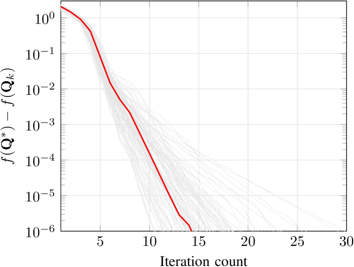
((a)) Degraded channels.

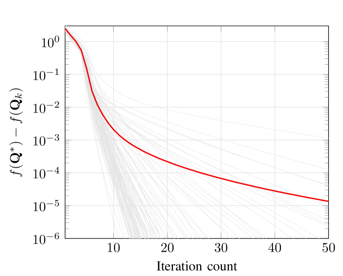
((b)) Non-degraded channels.

Figure 1: Convergence results of Algorithm 1. $N_{t}=N_{r}=N_{e}=4$ at $P_{t}=15$ dB.

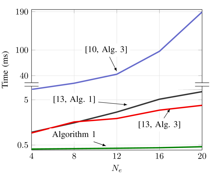
Figure 2: Time comparison of various algorithms for $N_{t}=4$ and $N_{r}=3$.

IV-B Convergence Analysis

We now show that the iterate sequence $\{\mathbf{Q}_{k}\}$ returned by Algorithm 1 converges to a stationary of (2). First, since $\nabla C_{s}(\mathbf{Q})$ is Lipschitz continuous, the backtracking line search terminates in an finite number of steps. More specifically, the number of line search steps at iteration $k\geq 1$ is bounded by $2+\log_{\gamma_{u}}\bigl{(}\beta_{k}/\beta_{k-1}\bigr{)}$. Now suppose that $C_{s}(\mathbf{Z}_{k})\geq C_{s}(\mathbf{Q}_{k})$ and $\mathbf{Z}_{k}$ is feasible. Then we have $\mathbf{Y}_{k+1}=\mathbf{Z}_{k}$ (cf. Line 1). The projection at iteration $k+1$ can be explicitly written as

$$\mathbf{Q}_{k+1} = \Pi_{\mathcal{\mathcal{Q}}}\bigl{(}\mathbf{Z}_{k}+\tfrac{1}{\beta_{k}}\nabla C_{s}(\mathbf{Z}_{k})\bigr{)}$$ (28a)

$$= \underset{\mathbf{Q}\in\mathcal{\mathcal{Q}}}{\arg\min}\ \bigl{\|}\mathbf{Q}-\mathbf{Z}_{k}-\tfrac{1}{\beta_{k}}\nabla C_{s}(\mathbf{Z}_{k})\bigr{\|}^{2}$$ (30a)

$$=\underset{\mathbf{Q}\in\mathcal{\mathcal{Q}}}{\arg\min}\ \tfrac{\beta_{k}}{2}\bigl{\|}\mathbf{Q}-\mathbf{Z}_{k}\bigr{\|}^{2}-\operatorname{tr}\bigl{(}\nabla C_{s}(\mathbf{Z}_{k})\bigl{(}\mathbf{Q}-\mathbf{Z}_{k}\bigr{)}\bigr{)}.$$

Note that (30a) implies

$$\tfrac{\beta_{k}}{2}\bigl{\|}\mathbf{Q}_{k+1}-\mathbf{Z}_{k}\bigr{\|}^{2}-\operatorname{tr}\bigl{(}\nabla C_{s}(\mathbf{Z}_{k})\bigl{(}\mathbf{Q}_{k+1}-\mathbf{Z}_{k}\bigr{)}\bigr{)}\leq 0.$$ (31)

It follows from the condition in Line 1 that

$$C_{s}(\mathbf{Q}_{k+1})\geq\mu_{\beta_{k}}(\mathbf{Z}_{k};\mathbf{Q}_{k+1})=C_{s}(\mathbf{Z}_{k})$$

$$+\operatorname{tr}\bigl{(}\nabla C_{s}(\mathbf{Z}_{k})\bigl{(}\mathbf{Q}_{k+1}-\mathbf{Z}_{k}\bigr{)}-\tfrac{\beta}{2}\bigl{\|}\mathbf{Q}_{k+1}-\mathbf{Z}_{k}\bigr{\|}^{2}$$ (32)

which, by using (31), yields

$$C_{s}(\mathbf{Q}_{k+1})\geq C_{s}(\mathbf{Z}_{k})\geq C_{s}(\mathbf{Q}_{k}).$$ (33)

Similarly, if $\mathbf{Y}_{k+1}=\mathbf{Q}_{k}$, then we can also prove that $C_{s}(\mathbf{Q}_{k+1})\geq C_{s}(\mathbf{Q}_{k})$ following the same procedure. Note that the inequality is strict if $\mathbf{Q}_{k+1}\neq\mathbf{Q}_{k}$. By noting that the feasible set is compact convex, we can conclude the objective sequence $\{C_{s}(\mathbf{Q}_{k})\}$ is convergent and there exists a subsequence $\{\mathbf{Q}_{k}\}$ converging to a limit point $\mathbf{Q}^{\ast}$. The proof that $\mathbf{Q}^{\ast}$ is a stationary point of (2) is standard and thus omitted here for the sake of brevity [16].

V Numerical Results

To illustrate Theorem 1 and also the convergence rate of Algorithm 1, we plot the residual error (i.e., $C_{s}-C_{s}(\mathbf{Q}_{k})$) for both degraded and non-degraded channels in Figs. 1(a) and 1(b), respectively. The channels $\mathbf{H}$ and G are generated as $\mathcal{CN}(\mathbf{0,I})$. The secrecy capacity $C_{S}$ is found using existing optimal algorithms. More specifically, for the degraded MIMO WTC, problem (2) can be reformulated as a standard semidefinite program and thus can be optimally solved by off-the-shelf solvers such as MOSEK [19]. For the non-degraded case, we implement the barrier method [10, Alg. 3] and [13, Alg. 3], both of which can find the secrecy capacity but are based on the equivalent convex-concave reformulation. Note that Algorithm 1 is applied to problem (2) directly. As can be seen clearly in Fig. 1, Algorithm 1 achieves monotonic convergence as proved in (33). Also, the residual error is reduced quickly to zero as the iteration process continues for both degraded and non-degraded cases. These results indeed confirm that Algorithm 1, even when applied to the nonconvex form of the secrecy capacity problem, can still compute the optimal solution, which is explained by Theorem 1.

To further demonstrate the benefit of Theorem 1 and Algorithm 1, in Fig. 2, we compare the run time of Algorithm  1 as a function of the number of the antennas at Eve. The simulation codes are built on MATLAB and executed in a 64-bit Windows PC system with 16 GB RAM and Intel Core-i7, 3.20 GHz processor. We plotted the average actual run-time for 200 different channel realizations. The stopping criteria for all the algorithms is when the increase in the resulting objective is less than $10^{-5}$ during the last 5 iterations. We can see our proposed algorithm outperforms other known methods such as [13, Algorithm 1 and 3] and [10, Algorithm 3] in terms of time complexity.

VI Conclusion

We have proved that the secrecy rate maximization problem of the general MIMOME WTC (i.e. no assumption is made on whether the channel is degraded) under a sum power constraint, despite its non-convexity, has a unique KKT solution. The proof basically implies that any local optimization method that aims to find a stationary solution can indeed solve secrecy capacity problem for non-degraded MIMO wiretap channels which are known to be non-convex. Motivated by this interesting result, we have also presented an accelerated projected gradient method with adaptive momentum to solve the secrecy problem. Simulation results have demonstrated that the proposed algorithm can find the optimal solution very fast.

[Lipschitz constant of $\nabla C_{s}(\cdot)$ ]Recall that $L>0$ is a Lipschitz constant of $\nabla C_{s}(\mathbf{Q})$ on $\mathcal{\mathcal{Q}}$ if the following inequality holds

$$\bigl{\|}\nabla C_{s}(\mathbf{X})-\nabla C_{s}(\mathbf{\mathbf{Y}})\bigr{\|}\leq L\bigl{\|}\mathbf{X}-\mathbf{Y}\bigr{\|},\forall\mathbf{\mathbf{X}},\mathbf{Y}\in\mathcal{\mathcal{Q}}.$$ (34)

Using (4) and the norm inequality, it is easy to see that

$$\bigl{\|}\nabla C_{s}(\mathbf{X})-\nabla C_{s}(\mathbf{Y})\bigr{\|}\leq$$

$$\bigl{\|}\mathbf{H}^{{\dagger}}\bigl{(}\mathbf{I}+\mathbf{H}\mathbf{\mathbf{X}}\mathbf{H}^{{\dagger}}\bigr{)}^{-1}\mathbf{H}\bigl{(}\mathbf{Y}-\mathbf{X}\bigr{)}\mathbf{H}^{{\dagger}}\bigl{(}\mathbf{I}+\mathbf{H}\mathbf{Y}\mathbf{H}^{{\dagger}}\bigr{)}^{-1}\mathbf{H}\bigr{\|}+$$

$$\bigl{\|}\mathbf{G}^{{\dagger}}\bigl{(}\mathbf{I}+\mathbf{G}\mathbf{X}\mathbf{G}^{{\dagger}}\bigr{)}^{-1}\mathbf{G}\bigl{(}\mathbf{Y}-\mathbf{X}\bigr{)}\mathbf{G}^{{\dagger}}\bigl{(}\mathbf{I}+\mathbf{G}\mathbf{Y}\mathbf{G}^{{\dagger}}\bigr{)}^{-1}\mathbf{G}\bigr{\|}.$$ (35)

We now recall the following well known inequality:

$$||\mathbf{A}\mathbf{B}|| \leq\lambda_{\max}(\mathbf{A})||\mathbf{B}||$$ (36)

where $\lambda_{\max}(\cdot)$ denotes the maximum singular value of the matrix in the argument. Applying the above inequality and by noting that $\lambda_{\max}\Bigl{(}\bigl{(}\mathbf{I}+\mathbf{H}\mathbf{\mathbf{X}}\mathbf{H}^{{\dagger}}\bigr{)}^{-1}\Bigr{)}\leq 1$ we have

$$\bigl{\|}\nabla C_{s}(\mathbf{X})-\nabla C_{s}(\mathbf{Y})\bigr{\|} \leq\bigl{(}\sigma\bigl{(}\mathbf{H}^{{\dagger}}\mathbf{H}\bigr{)}+\sigma_{\max}^{2}\bigl{(}\mathbf{G}^{{\dagger}}\mathbf{G}\bigr{)}\bigr{)}\bigl{\|}\mathbf{X}-\mathbf{Y}\bigr{\|}$$

which means that $L=\sigma_{\max}^{2}\bigl{(}\mathbf{H}^{{\dagger}}\mathbf{H}\bigr{)}+\sigma_{\max}^{2}\bigl{(}\mathbf{G}^{{\dagger}}\mathbf{G}\bigr{)}$ is a Lipschitz constant of $\nabla C_{s}(\cdot)$.

References

• [1] A. D. Wyner, “The wire-tap channel,” Bell System Technical Journal, vol. 54, no. 8, pp. 1355–1387, 1975.
• [2] S. Leung-Yan-Cheong and M. Hellman, “The Gaussian wire-tap channel,” IEEE Trans. Inf. Theory, vol. 24, no. 4, pp. 451–456, Jul. 1978.
• [3] Z. Li, W. Trappe, and R. Yates, “Secret communication via multi-antenna transmission,” in 41st Annual Conference on Information Sciences and Systems 2007, Mar. 2007, pp. 905–910.
• [4] A. Khisti and G. W. Wornell, “Secure transmission with multiple antennas I: The MISOME wiretap channel,” IEEE Trans. Inf. Theory, vol. 56, no. 7, pp. 3088–3104, Jun. 2010.
• [5] ——, “Secure transmission with multiple antennas part II: The MIMOME wiretap channel,” IEEE Trans. Inf. Theory, vol. 56, no. 11, pp. 5515–5532, Oct. 2010.
• [6] F. Oggier and B. Hassibi, “The secrecy capacity of the MIMO wiretap channel,” IEEE Trans. Inf. Theory, vol. 57, no. 8, pp. 4961–4972, Aug 2011.
• [7] S. Fakoorian and A. L. Swindlehurst, “Full rank solutions for the MIMO Gaussian wiretap channel with an average power constraint,” IEEE Trans. Signal Process., vol. 61, no. 10, pp. 2620–2631, Mar. 2013.
• [8] Q. Li, M. Hong, H.-T. Wai, Y.-F. Liu, W.-K. Ma, and Z.-Q. Luo, “Transmit solutions for MIMO wiretap channels using alternating optimization,” IEEE J. Sel. Areas Commun., vol. 31, no. 9, pp. 1714–1727, Sep. 2013.
• [9] J. Steinwandt, S. A. Vorobyov, and M. Haardt, “Secrecy rate maximization for MIMO Gaussian wiretap channels with multiple eavesdroppers via alternating matrix POTDC,” in Proc. IEEE ICASSP 2014, May 2014, pp. 5686–5690.
• [10] S. Loyka and C. D. Charalambous, “An algorithm for global maximization of secrecy rates in Gaussian MIMO wiretap channels,” IEEE Trans. Commun., vol. 63, no. 6, pp. 2288–2299, Jun. 2015.
• [11] S. Loyka and C. D. Charalambous, “Optimal signaling for secure communications over Gaussian MIMO wiretap channels,” in IEEE Trans. Inf. Theory, vol. 62, no. 12, Dec. 2016, pp. 7207–7215.
• [12] T. V. Nguyen, Q.-D. Vu, M. Juntti, and L.-N. Tran, “A low-complexity algorithm for achieving secrecy capacity in MIMO wiretap channels,” in Proc. IEEE ICC 2020, Jun. 2020.
• [13] A. Mukherjee, B. Ottersten, and L.-N. Tran, “Efficient numerical methods for secrecy capacity of Gaussian MIMO wiretap channel,” in Proc. IEEE VTC 2021, May 2021. [Online]. Available: https://arxiv.org/abs/2102.10396
• [14] ——, “On the MIMO secrecy capacity of MIMO wiretap channels: Convex reformulation and efficient numerical methods,” submitted to IEEE Trans. Commun., 2020. [Online]. Available: https://arxiv.org/abs/2012.05667
• [15] D. S. Bernstein, Matrix Mathematics: Theory, Facts, and Formulas (Second Edition).   Princeton University Press, 2009.
• [16] Q. Li, Y. Zhou, Y. Liang, and P. K. Varshney, “Convergence analysis of proximal gradient with momentum for nonconvex optimization,” in Proc. the 34th International Conference on Machine Learning, vol. 70.   PMLR, Aug. 2017, pp. 2111–2119. [Online]. Available: http://proceedings.mlr.press/v70/li17g.html
• [17] Y. Nesterov, “Gradient methods for minimizing composite functions,” Math. Program., vol. 140, pp. 125–161, 2013.
• [18] S. Ye and R. Blum, “Optimized signaling for MIMO interference systems with feedback,” IEEE Trans. Signal Process., vol. 51, no. 11, pp. 2839–2848, Nov. 2003.
• [19] M. ApS, The MOSEK optimization toolbox for MATLAB manual. Version 9.2, 2020. [Online]. Available: https://docs.mosek.com/9.2/toolbox/index.html