GraphSAT – a decision problem connecting satisfiability and graph theory
GraphSAT – a decision problem connecting satisfiability and graph theory
Abstract.
Satisfiability of boolean formulae (SAT) has been a topic of research in logic and computer science for a long time. In this paper we are interested in understanding the structure of satisfiable and unsatisfiable sentences. In previous work we initiated a new approach to SAT by formulating a mapping from propositional logic sentences to graphs, allowing us to find structural obstructions to 2SAT (clauses with exactly 2 literals) in terms of graphs. Here we generalize these ideas to multi-hypergraphs in which the edges can have more than 2 vertices and can have multiplicity. This is needed for understanding the structure of SAT for sentences made of clauses with 3 or more literals (3SAT), which is a building block of NP-completeness theory. We introduce a decision problem that we call GraphSAT, as a first step towards a structural view of SAT. Each propositional logic sentence can be mapped to a multi-hypergraph by associating each variable with a vertex (ignoring the negations) and each clause with a hyperedge. Such a graph then becomes a representative of a collection of possible sentences and we can then formulate the notion of satisfiability of such a graph. With this coarse representation of classes of sentences one can then investigate structural obstructions to SAT. To make the problem tractable, we prove a local graph rewriting theorem which allows us to simplify the neighborhood of a vertex without knowing the rest of the graph. We use this to deduce several reduction rules, allowing us to modify a graph without changing its satisfiability status which can then be used in a program to simplify graphs. We study a subclass of 3SAT by examining sentences living on triangulations of surfaces and show that for any compact surface there exists a triangulation that can support unsatisfiable sentences, giving specific examples of such triangulations for various surfaces.
1. Introduction
We introduce and analyze a novel graph decision problem that we call GraphSAT. Using the tools of graph theory, this new variant builds upon the classical logic and computer science problem of boolean satisfiability (sat). sat asks if there exists a truth assignment that satisfies a given boolean formula. Our variant deals with multi-hypergraphs instead of boolean formulae and uses truth assignments on vertices instead of variables. This graph-theoretic picture helps us explore and exploit patterns in unsatisfiable instances of sat, which in turn helps us identify minimal obstruction sets to graph satisfiability.
In Theorem 3.5 (the local rewriting theorem) we prove invariance of graph satisfiability under a graph rewriting system that we introduce. This theorem is the main conceptual and computational tool that allows us to replace the question of satisfiability of a graph by those for smaller graphs. This theorem makes possible a computational search for patterns in satisfiable and unsatisfiable graphs without knowing the entirety of the graph. The computational results in this paper, for example the search for unsatisfiable instances of GraphSAT, were obtained using a Python package (called graphsat) that we created to handle multi-hypergraph instances and local rewriting of graphs. This software will be described elsewhere. Our goal in this paper is to introduce GraphSAT and logical operations on graphs and to prove the local graph rewriting theorem as well as to detail consequences of this theorem.
This paper is a successor to [2], which looks at GraphSAT restricted to multi-graphs and sat. The key results in that paper are that graph homeomorphisms preserve satisfiability status and a complete set of minimal unsatisfiable simple graphs. Specifically, we showed that there are exactly four obstructions to satisfiability in simple graphs and exactly four obstructions to satisfiability in looped-multi-graphs.
Theorem (Theorem 18 and Remark 19 in [2]).
A simple graph is unsatisfiable if and only if it contains an element of the set
as a topological minor. A looped-multi-graph is unsatisfiable if and only if it contains an element of the set
as a topological minor.
This current paper is the first step towards generalizing the sat results of [2] to sat. By studying properties of satisfiable and unsatisfiable graphs we are studying entire classes of boolean formulae. This results in a coarsening compared to studying Cnfs directly. Nevertheless, the translation from Cnfs to graphs capture the essential features of any formula and offers a complete picture of the structure of its boolean constraints. For example, we show that this notion of satisfiability is closed under subgraphing as well as under the relations of “shaved graph versions” and topological-minoring. The family of satisfiable multi-hypergraphs is also closed under the action of a variety of higher-dimensional analogues of well-known graph operations. We explore these analogous graph operations and analyze their effects vis-à-vis the structural properties of multi-hypergraphs.
Robertson and Seymour, in their seminal papers [6] proved that a graph family that is closed under the graph minor operation always has a finite obstruction set. This theorem also does not apply to the case of graphs for sat considered in [2]. Despite this, in [2], we were able to obtain a very short list of obstructions listed in the Theorem above. The case of sat for considered here is considerably harder. There is no known finite obstruction Robertson-Seymour theorem for multi-hypergraphs. Nevertheless, we obtain several hundred obstructions to satisfiability for multi-hypergraphs. We enumerate a part of this list in Appendix C.
Section 2 introduces definitions and notations used in this paper. It introduces some type-theoretic notation that streamlines the mathematical exposition. It also includes definitions for the two halves of GraphSAT, i.e. boolean formulae and graphs.
In Section 3 we state and prove the local graph rewriting theorem (Theorem 3.5), that enables rewriting of graphs at a vertex, while preserving its satisfiability status. In Section 4 we list some graph rewrite rules that leave graph satisfiability invariant. In 4.1 we give a result that is true for edges of any size. Thereafter, we restrict our attention to edges of size at most three. In Sections 5, 6 and 7 we consider the satisfiability of mixed hypergraphs, triangulations, and infinite graphs respectively. In these sections we summarize some of the key findings enabled by the local rewriting theorem (Theorem 3.5), and by our graphsat Python package. This software package along with the local rewriting theorem allows us to conduct experiments combining programming and proofs to classify graphs, hypergraphs, and infinite graphs as totally satisfiable or unsatisfiable. Section 8 provides a conclusion to this study by summarizing key results as well as future directions and conjectures.
2. Definitions and notation
We start by inductively defining boolean formulae in conjunctive normal form in §2.2 and graphs (in fact multi-hypergraphs) in §2.5. We introduce a way to view graphs as sets of Cnfs in §2.5.1. After translating Cnfs to graphs, we also define a notion of satisfiability for graphs in §2.5.2. We also define notation and conventions aimed at making the connection between Cnfs and graphs more intuitive. These are summarized in Table 4.
2.1. Type theory annotations
Throughout this section, we add various annotations to our terms in order to aid the reader in parsing and understanding the mathematics presented herein. These annotations are inspired from the field of type theory and can be thought of as representing the “category” or the “type” of a term.
For example, we write to mean is of type Clause and is equal to . The type annotations help with clarity without changing the mathematical content. For this reason, we use them wherever they can add to the exposition and avoid them wherever they might be unnecessarily verbose.
We will use a fixed list of types in this section, collected in Table 1. Full definitions for each type can be found in the sections that follow. Let denote an arbitrary type, used to parameterize the other types. Elements of will be called variables. For example, we define the type to be the type of all Cnfs on the variable set . In practice, we will avoid mentioning explicitly and simply write type judgments like instead of .
In Table 1, we use the notation to be mean that the two types have exactly the same terms. We write to mean that is a subtype of . This indicates that there are some extra restrictions placed on . For example, we have because every clause can also be viewed as a set of literals. However, not every set of literals is a clause because we require that clauses be nonempty. We also use and to denote the disjoint-sum and Cartesian-product of types respectively.
| Type | Relation to other types | Description |
|---|---|---|
| Variable | Variable | variables; an alias of |
| Literal | Literal Bool | literals of variable type |
| Clause | Clause Set Literal | clauses of variable type |
| Cnf | Cnf Set Clause | Cnfs of variable type |
| Assignment | Assignment Set Literal | assignment of variable type |
| Vertex | Vertex | vertices; an alias of |
| Edge | Edge Set Vertex | hyperedges of vertex type |
| Graph | Graph Multiset Edge | multi-hypergraphs of vertex type |
| Bool | the type of boolean values (true and false) | |
| the type of natural numbers | ||
| Set | homogeneous sets of elements of type | |
| Multiset | Multiset | homogeneous multi-sets of elements of type |
2.2. Boolean formulae
In this section, we inductively define variables, literals, clauses, Cnfs and assignments. We then define satisfiability and equi-satisfiability for Cnfs.
We fix an arbitrary countable set and call its elements variables. Variables will be denoted by etc. We denote the type of variables as Variable and thus can write to mean that is a variable.
A literal is either a variable, denoted by the same symbol as the variable; or its negation, denoted by or . We also declare that there are two additional literals called true (denoted by ) and false (denoted by ).
We denote the type of literals as Literal and can thus write to mean that is a literal. The Literal type is thus composed of two copies of and one copy of true and false. We can therefore write Literal .
A clause is a disjunction of one or more literals. A clause made of a single literal is also denoted by . We denote the type of clauses as Clause. Thus, the following are all valid examples of clauses — .
A Cnf is a boolean formula in conjunctive normal form, i.e. it is a formula made of conjunction of one or more clauses. A Cnf containing a single clause has the same representation as the clause itself. Thus, the following are all valid Cnfs — .
2.3. Assignments
A truth assignment (or simply an assignment) is a set of literals with the additional condition that a literal and its negation cannot both belong to an assignment. We denote the type of assignments by Assignment.
We define the action of a singleton assignment on a Cnf to be the Cnf formed by replacing every occurrence of in with and every occurrence of in with . We define the action of a general assignment on a Cnf to be the Cnf formed by the successive action of each element of on . We denote this new Cnf by .
For example, .
We simplify this notation by writing instead of .
2.4. Satisfiability of Cnfs
A Cnf is satisfiable if there exists a truth assignment such that . Otherwise, is unsatisfiable. Two Cnfs and are equi-satisfiable (denoted ) if either they are both satisfiable or they are both unsatisfiable. We write or to denote that is satisfiable or unsatisfiable respectively.
We also introduce a map for Cnf-satisfiability denoted , which maps satisfiable Cnfs to and unsatisfiable Cnfs to .
We note that assigning a literal to does not change the satisfiability status of a Cnf , i.e .
2.5. Graphs and Satisfiability
In this section we define graphs inductively starting with vertices and then building up through edges (looped, simple and hyper) and then multi-edges. The standard term for these graph objects would be “looped-multi-hypergraphs”. We then define a novel way of interpreting a graph as a set of Cnfs that can “live on that graph”. This translation of graphs into sets of Cnfs is lies at the heart of our attempt to turn boolean satisfiability instances into graph theory problems. Consequently, we make this translation as explicit as possible and provide enough details so that the interested reader may generate a translation “algorithm” from our definitions to readily turn any graph into a set of Cnfs.
Let be a countable set of vertices. We will omit any mention of a specific and simply denote its elements using boldface symbols . A hyperedge (or simply an edge) on is a nonempty set of vertices. We omit the surrounding braces while denoting edges and simply write the vertices in a contiguous fashion. For example, , and denote edges of size one (a loop), two (a simple edge) and three (a triangle) respectively.
A graph on is a nonempty multiset of edges on . In literature, these are typically referred to as multi-hypergraphs or looped-multi-hypergraphs, but we simply call them graphs. When listing the edges of a graph, we omit the surrounding braces and wrap each edge in parentheses, listing them one after the other. For example, . If an edge repeats in a graph, we denote its multiplicity as a superscript. For example, .
The degree of a vertex in an edge is if the vertex is an element of the edge, and otherwise. The degree of a vertex in a graph is the sum of the degrees of the vertex over all edges of the graph, while counting multiplicities as distinct edges. We note that we draw a loop as an edge starting an ending at the same vertex, but this is still considered to contribute only to the degree count of said vertex.
2.5.1. Graphs as sets of Cnfs
We define the functions as follows —
-
•
, such that
-
•
, such that
-
•
, such that
-
•
, such that
The image of an edge under gives us the set of all Cnfs that “live on that edge”. There are Cnfs in the set corresponding to an edge of size with multiplicity . The image of a graph under gives us the set of all Cnfs that “live on that graph”. We use this set often enough that we will simply omit writing , and and we will conflate the graph with its set of Cnfs. For example, the following graph is also a set.
Therefore, when we write set operations on graphs, say like , we really mean .
We further define two special sets of Cnfs, which we denote by boldface true and false symbols
-
•
-
•
Note that both of these are sets of Cnfs that are not graphs (due to the requirement that a graph be a nonempty multiset of edges). Similarly, the empty set is also a valid term of type Set Cnf but is not a valid term of type Graph.
The set of Cnfs living on a graph can sometimes be empty. For example, the following graphs correspond to empty sets — . These sets are empty because their image under is empty. In general, a graph is empty if and only if it has an edge of size with multiplicity more than .
2.5.2. Graph equi-satisfiability
A set of Cnfs is totally satisfiable if it is nonempty and if every Cnf in it is satisfiable. Otherwise, it is unsatisfiable. We denote by , the map that sends a Graph to if it is totally satisfiable, and to otherwise. We note that for any set of Cnfs and , we have .
Two sets of Cnfs and are equi-satisfiable if they are both totally satisfiable or are both unsatisfiable. We write this as .
We say that equi-implies by the -criterion (denoted ) if, . If both and , then we denote this more compactly as .
We say that equi-implies by the -criterion (denoted ) if, . If both and , then we denote this more compactly as .
Remark 2.1.
The idea of graph equi-satisfiability is not necessarily useful for a specific pair of graphs, but it is useful for discovering operations that preserve satisfiability like when a part of the graph structure is fixed and not changing.
2.5.3. The GraphSAT decision problem
GraphSAT is the graph decision problem that asks if a given looped-multi-hypergraph is totally satisfiable.
-
•
Instance: Given a specific looped-multi-hypergraph .
-
•
Question: Is every Cnf such that satisfiable.
GraphSAT is a restriction of GraphSAT that only allows looped-multi-hypergraphs with hyperedge sizes at most .
In [2] we enumerated a complete list of minimal unsatisfiable simple graphs and a proof that GraphSAT is in complexity class P. We might hope for a similar complete list for GraphSAT, and perhaps a different complexity class for GraphSAT. Unfortunately, this is not the case. The GraphSAT problem is more complicated for three main reasons —
-
(1)
The minimality of the GraphSAT list hinged on homeomorphisms (i.e. edge-subdivisions) preserving graph satisfiability. There is no single analogue of homeomorphisms, edge-subdivisions, and topological minoring in the case of hypergraphs.
-
(2)
Bruteforce checking of the satisfiability status of a graph is not a sustainable option for GraphSAT owing to the large number of Cnfs supported by a typical looped-multi-hypergraph.
-
(3)
In studying GraphSAT, we argued (in [2]) that we can always reduce higher multiplicity edges down to . This was because a multiplicity edge is always unsatisfiable, a multiplicity edge forces an assignment on its vertices, and a multiplicity edge forces an equivalence on its vertices. Such a complete result does not exist for hyperedges. The best we can do is to say that a multiplicity hyperedge is always unsatisfiable, and a multiplicity hyperedge forces assignments on its vertices.
These factors conspire to make GraphSAT a harder problem to solve, but also yield richer structures and relations between various multi-hypergraphs and their satisfiability statuses.
2.5.4. Disjunction and conjunction of graphs
We define disjunction for sets of Cnfs to be a binary operation such that
where, , is a map that converts boolean formulae into Cnfs by repeatedly using distributivity of disjunction over conjunction. We note that this is only one of several possible implementations of . We choose this implementation because it has the advantage of not introducing any new variables. In a computer implementation of , the use of distributivity is inefficient. But, since we are concerned only with small graphs, this is not an issue. We write instead of .
We define conjunction for sets of Cnfs to be a binary operation such that . We write instead of .
We note that disjunction of graphs need not result in a graph, while conjunction of graphs always does. We now list some properties of graph disjunction, graph conjunction and equi-satisfiability.
Proposition 2.1.
Let and be sets of Cnfs.
-
(1)
if and only if .
In other words, we can restrict our attention to only finding unsatisfiable Cnfs in both sets in order to prove their equi-satisfiability. -
(2)
implies for every .
In other words, equi-implication by the -criterion is a stronger condition than the -criterion. -
(3)
implies for every .
-
(4)
implies , for every .
In other words, particularly when dealing with graphs, we can factor out the largest common subgraph and restrict our attention to finding Cnfs on the remaining edges in order to prove graph equi-satisfiability. -
(5)
, and similarly, .
-
(6)
If both and are unsatisfiable, then we can conclude that is also unsatisfiable.
-
(7)
If we take our arrows to be equi-implications under the criterion, then graph disjunction obeys the universal property of products, while union of Cnf sets possesses the universal property of sums.
-
(a)
If and , then .
-
(b)
If and , then .
-
(a)
-
(8)
Let be a set of Cnfs. If either one of or is totally satisfiable, then, so is .
-
(9)
implies , for every . Proposition 2.1.
Proof.
-
(1)
Suppose that . If both sets are totally satisfiable, then the statement is vacuously true. If both sets are unsatisfiable, then for every unsatisfiable Cnf in , we choose an unsatisfiable Cnf in . Similarly, for every unsatisfiable Cnf in , we can choose a corresponding unsatisfiable Cnf in , thus satisfying the requirements of the -criterion of equi-implication. Conversely, if , then given an unsatisfiable Cnf in we can obtain an unsatisfiable Cnf in . Thus, either both sets are totally satisfiable or both are unsatisfiable.
-
(2)
Proof follows from definition of the - and -criterions of equi-implication.
-
(3)
If either , , or is empty, the conclusion is vacuously true. Let us suppose then that these sets are all nonempty. Let be an element of . Using the hypothesis, we can obtain a Cnf such that is falsified by every assignment that falsifies .
Any assignment that falsifies also falsifies . We have therefore proved that equi-implies by the -criterion.
- (4)
-
(5)
Let . We can factor as for some and , such that and . We choose . Then, any assignment that falsifies falsifies both and . In particular, any such assignment also falsifies .
-
(6)
Let and be unsatisfiable Cnfs. Any assignment that satisfies must also satisfy either or or both. Hence, we can conclude that no assignment satisfies . This proves that is unsatisfiable.
-
(7)
For (a), we note that for every , there exist Cnfs and such that any assignment that falsifies also falsifies both and . Thus, any assignment that falsifies also falsifies . For (b), we note that for every , there exists a Cnf such that any assignment that falsifies also falsifies . This covers every Cnf in coming from . A similar argument hold for every Cnf coming from . This proves that .
-
(8)
Suppose is unsatisfiable. Then, there exist Cnfs , , and such that is unsatisfiable. Then, both and . In other words, both and are unsatisfiable.
-
(9)
It suffices to show that . follows from 7b. is trivially true.
∎
Remark 2.2.
We note that graph conjunction and graph disjunction have several familiar properties while also missing several properties that we are used to.
-
(1)
Both operations are commutative and associative.
-
(2)
The operations do not obey distributivity laws, i.e. for general sets or Cnfs and ,
-
(a)
. In fact, we have . To see that this is a proper subset, we can merely count the number of Cnfs on both sides. The left side has Cnfs, where is the cardinality of the set , while the right side has Cnfs.
-
(b)
. In fact, we have . To see that this is a proper subset, we count Cnfs on the left side, while the right side has Cnfs.
-
(a)
2.5.5. Graph disjunction does not always result in graphs
Essential to carrying out local graph rewriting (detailed in §3) is the calculation of graph disjunctions of the form . A graph disjunction, even if we start with and being graphs, frequently yields a set of Cnfs that might not be a graph. For example,
We note that these three Cnfs do not belong to the set corresponding to any single graph because the Cnfs do not have the same vertex set. The Cnfs and have a vertex set of ; the true Cnf has an empty vertex set. Nevertheless, we can write it as a union of graphs. We can write .
Nevertheless, we cannot always write a disjunction even as a union of graphs. For example,
Although the remaining Cnfs all belong to the same graph, namely , we note that we do not have the complete set. For example, we are missing the Cnf . Hence we cannot write . The best we can do is —
These subset-superset pairs give us a lower and upper bound for the set in the middle. The utility of these subset-superset pairs becomes apparent when we view them in the context of satisfiability statuses. In the following equation, let an arbitrary graph. Then, we have —
This means that if is unsatisfiable, then is too. On the other hand, if is totally satisfiable, then by checking if is also totally satisfiable, we can conclude that is totally satisfiable as well. This is a technique that we often use since the graph disjunction does not always yield a union of graphs.
We include tables of such standard graph disjunctions in Appendix B. These tables come in handy performing local rewrites, as seen in §4. The first two tables list graph disjunctions that can be written exactly as a union of graphs; the third table lists graph disjunctions that can only be listed as a subset-superset pair.
3. Local rewriting in graphs
Graph rewriting concerns the technique of creating a new graph out of an original graph algorithmically. Formally, a graph rewriting system consists of a set of graph rewrite rules of the form . The idea is that to apply the rule to a graph , we search for the presence of a subgraph of and replace the subgraph with while leaving the rest unchanged. Such rewrite rules come in two forms —
-
(1)
Local rules — when a graph is rewritten at a particular vertex. In this case, all edges not adjacent to the vertex remain unaffected by the rewrite.
-
(2)
Global rules — when a graph is rewritten by searching for specific subgraphs that are isomorphic to .
We will concern ourselves with local rules in this section, while global rules will be handled by §4.
We are looking for hypergraph analogue(s) of edge-subdivisions/edge-smoothing in order to define the corresponding notion of minimality in GraphSAT. This leads us naturally into local rewriting, i.e. operations where change the graph at a single vertex and its neighborhood. The idea is to find changes or rewrites that leave the satisfiability of a graph unchanged. For example, edge-subdivision can be though of as the rewrite , while the inverse operation of edge smoothing can be thought of as . Using local rewriting, we try to generalize this rule as well as the proof that it leave the satisfiability of a graph unchanged.
For local rules, we focus on the extended notion of “making assignments” detailed in §3.1. Just as for a Cnf , denotes its an assignment at a literal , we write to denote assignment at a vertex of a graph .
Literal assignments on Cnfs have two key properties that make them useful –
-
(1)
If is a Cnf and is a literal that is in the set of literals of , then is guaranteed to be smaller than – it either has fewer clauses, or it has the same number of clauses but with those clauses having fewer literals in them.
-
(2)
is satisfiable if and only if either one of or are satisfiable.
Vertex assignments on graphs also have similar properties —
-
(1)
If is a graph and is a vertex in the vertex set of , then will always have Cnfs that are smaller than the Cnfs in .
-
(2)
is totally satisfiable if and only if is totally satisfiable.
This operation of vertex assignment is defined rigorously in §3.1. The local graph rewriting theorem (Theorem 3.5) presents an alternate expression for computing that is easier to write when performing calculations, easier to code when programming it into a computer, and is a form that is used for proving several global graph rewrite rules. The essence of this theorem is that even though satisfiability (both boolean and graph) is a global problem i.e. it is affected by the full structure of the Cnf, it can also be broken down into a series of local assignments in the case of Cnfs and a series of local rewrites in the case of graphs. Given a graph, we can decompose it at one of its vertices of by computing this alternate expression in terms of the link and rest of the graph without needing to step down to the level of Cnfs. We close this section with a discussion on some consequences of this theorem and an implementation of local rewriting in code (as a part of graphsat).
Remark 3.1.
We note that replacing a part of a CNF with an equisatisfiable part breaks the equi-satisfiability of the whole CNF. For example, even though is equisatisfiable to , we cannot replace with , since the former is unsatisfiable while the latter is satisfiable.
However, in graphs, replacing some special subgraphs with equisatisfiable pieces preserves equi-satisfiability. This is the basis for finding rewrite rules using the local rewriting theorem (Theorem 3.5.
3.1. Assignments on graphs
For a clause or Cnf, we defined assignments at a literal in §2.3. We now define assignments for a graph at a vertex. We note that this is a completely new notion that does not exists in graph theory and can be defined here only because of the connection we have established between graphs and Cnfs in the previous sections.
Let be a vertex, and be a graph. We define,
We note here that despite what the notation might suggest, is in general not an element of . If , then is in fact an element of the graph . The definitions of link and rest can be found in §3.2.
Next, we prove that assignments on graphs do not alter their satisfiability status. This is useful because post-assignment the graphs always result in sets with Cnfs having one fewer variable, while not altering their satisfiability status.
Lemma 3.1.
Let be a graph and let be a vertex. Then, .
Proof.
From the definition of , we know that .
First, we note that each is equisatisfiable to and each is equisatisfiable to . Thus, we can write , using the fact that disjunction of equisatisfiable Cnfs is equisatisfiable.
Next, we note that we can replace each Cnf of the set with an equisatisfiable Cnf without affecting the satisfiability status of the set. Thus, we write . ∎
3.2. Parts of a graph
We now define some parts of graphs that will be useful for stating the local rewriting theorem (Theorem 3.5). Let be a graph and let be a vertex.
-
•
The star of at a vertex of is the graph of all edges containing .
, where if and otherwise, i.e. we omit the edge otherwise. -
•
The link of at is the graph formed by removing from each edge of the star of at . In the following equation, denotes the usual set difference.
, where if and otherwise. Any edges with multiplicity or with size after deleting the vertex will simply be omitted from the resulting graph. -
•
The rest of at is the graph formed by all edges not containing . In other words, these are the edges of not contained in
, where if and otherwise, i.e. we omit the edge otherwise.
We note that when computing the -partitions of a multiset (for example a graph), we can split an edge with multiplicity across the partitions. This observation will come in handy when using the local rewriting theorem (Theorem 3.5). For example, we will consider to be a valid -partition of the graph .
A graph is a subgraph of a graph if every edge of (counting duplicates as distinct) is also an edge of . We denote this partial order on graphs by . An edge is a face of an edge if every vertex in is also in . A graph is a shaved version of a graph if can be constructed by replacing each edge of (counting duplicates as distinct) by a nonempty face of itself. We note that each graph is a shaved version of itself. We denote this partial order on graphs by .
We now prove some lemmas outlining the relation between subgraphs, shaved versions and satisfiability.
Lemma 3.2.
Let and be graphs such that . Then, .
Proof.
We can write for some . Let . Let be an arbitrary Cnf in . If is such that , then we have . ∎
Lemma 3.3.
Let and be edges such that is a face of . Then, .
Proof.
Let be arbitrary. We can write for some and some . Then, any assignment that falsifies necessarily falsifies , hence proving the result. ∎
Lemma 3.4.
Let and be graphs such that . Then, .
Proof.
We argue that the result follows for each face from the previous lemma. We can string these faces together to form the graphs while preserving equi-implication under the -criterion using Proposition 3. ∎
3.3. The local rewriting theorem
Theorem 3.5.
For every graph and every vertex with degree at least , we have the following equi-satisfiability relation.
| (1) |
For every vertex of with degree , we have .
Proof.
For vertices of degree , the theorem states that we can delete the single edge incident on without affecting the satisfiability status of . This is true because any can be written as or , where , and such that is a clause supported on the edge . Assigning to true and false respectively leaves us with the result , and thus .
We now consider the case where degree of in is at least . Since the star and the rest together form a partition of the edge set of a graph, we can write . Since we know from Lemma 3.1 that , we can also write .
Since graph conjunction is defined as the pairwise conjunction of the Cartesian product of underlying Cnfs, we can infer that graph disjunction commutes with set union. Thus, it suffices to show that
Suppose . Then, there exists a such that . Potentially, there are four types of clauses in — those that contain the literal , those that contain , contain both, or contain neither. The last two cases are not possible. A clause cannot contain both and because otherwise the edge corresponding to the clause will be incident on the vertex twice, which is something that the definition of an edge does not allow. A case where a clause contains neither nor is impossible because the Cnf belongs to the star of at .
We can therefore partition into containing clauses that contain , and containing clauses that contain , i.e. we can write . Thus, . Let and be the graphs that support and respectively. We have shown that . Furthermore, and form a -partition of since and form a -partition of the Cnf in . Generalizing this to all the different Cnfs in , we have shown that
Conversely, suppose , such that is some -partition of . Then, we can factor as , for some Cnfs and such that and . Consider then the Cnf given by . Firstly, we observe that . Secondly, we note that since the effect of disjuncting with is to extend each clause in and by a literal in . Thus, we can write . We have now shown that
∎
An implementation of the right side of (1) in Python using our graphsat package is in Appendix D. Details of the graphsat package will be provided in a separate publication. The source code of graphsat is available at [3].
Next, we will state two corollaries that can be turned into a test for satisfiable graphs. These corollaries are turned into procedures for testing the satisfiability status of a graph and are presented in detail later in this section.
Corollary 3.5.1.
Let be a graph and let be a vertex of . If is unsatisfiable, then there exists a -partition of such that both and are unsatisfiable.
Proof.
If is unsatisfiable, then so is the set for some -partition of . The result follows from Proposition 8. ∎
Corollary 3.5.2.
Let be a graph and let be a vertex of . If either one of or is totally satisfiable for every -partition of , then itself is totally satisfiable.
Proof.
This is the contrapositive of Corollary 3.5.1. ∎
The following procedures for checking graph satisfiability status use Corollary 3.5.2.
Procedure 3.1.
A non-recursive procedure for checking that a graph is totally satisfiable is as follows —
-
(1)
Pick a vertex of (the vertex of lowest degree will make the procedure easier).
-
(2)
Pick a -partition of , compute the satisfiability status of and . Satisfiability status of each graph can be checked using a graph satchecker (see §5).
-
(3)
If both are unsatisfiable then the result is inconclusive and we can exit the procedure (this follows from Remark 2.2). If either of these is totally satisfiable, then move on the next -partition and repeat Step 2.
-
(4)
If all -partitions have been exhausted, then is totally satisfiabile.
Note that in this procedure, once a vertex has been picked, the graphs used in Step 2 are both smaller than and do not use the vertex . Although the graphs in Step 2 are smaller, there are many more graphs to check since we have to check all possible -partitions. Hence, a naive application of Procedure 3.1 does not necessarily improve the efficiency of checking the satisfiability of a graph. The real application of this procedure is to serve as a step in the recursion outlined in the procedure below.
Procedure 3.2.
This procedure is a recursive version of Procedure 3.1. It checks the satisfiability status of a graph .
-
(1)
If is small, i.e. vertices or fewer, then check it using a graph satchecker (see §5). If is not small, we pick a vertex of (the vertex of lowest degree will make the procedure easier).
-
(2)
Pick a -partition of . Let and . We can think of as being the parent graph of its child graphs and .
-
(3)
The parent graph is totally satisfiable if either one of its child graphs is totally satisfiable (this follows from Corollary 3.5.2). To check satisfiability-status of each child graph , go back to Step 1. but with in place of and a vertex of in place of .
-
(4)
If both child graphs are unsatisfiable, then check the parent graph using a graph satchecker (see §5).
-
(5)
If either child graph is totally satisfiable, then conclude that their parent graph is satisfiable.
-
(6)
Once we have backtracked all the way back to the original graph , we can exit the procedure with a result of totally satisfiable or unsatisfiable.
This procedure has several advantages over Procedure 3.1. Firstly, the recursion creates smaller graphs, each of which can be checked more quickly. Secondly, unlike Procedure 3.1, Procedure 3.2 never returns an inconclusive result. However, this comes at the potential cost of having to backtrack all the way to the original graph and then having to sat-check the entire graph. Thirdly, the algorithm can be parallelized and memoized (storing and using the satisfiability statuses of graphs already seen when checking the satisfiability of new graphs). This helps in mitigating the potential slowdowns caused by having to now many graphs, since each recursion of Procedure 3.2 adds exponentially more graphs that need to be checked.
Procedure 3.3.
Procedure for checking satisfiability status of a graph using the process of “graph completion”.
-
(1)
Choose a vertex of (the vertex of lowest degree will make the procedure easier).
-
(2)
Compute the set of Cnfs
-
(3)
Construct a set of graphs for some index set such that . One way to construct this is to look at the image set of under the map that sends a Cnf to the graph that supports it. We call this process “graph completion”.
-
(4)
If every is totally satisfiable, then is totally satisfiable. If not, then is inconclusive.
-
(5)
To check the satisfiability status of , we can recursively call this procedure on each in place of .
We note that the run-time complexity of these procedures has not been analyzed.
The trouble with Procedures 3.1 and 3.3 is that it can only prove the total satisfiability of a graph. If the graph is unsatisfiable, then the procedure is inconclusive. It is possible to prove that a graph is totally satisfiable using this procedure, but not that it is unsatisfiable. This shortcoming can however be mitigated somewhat by our choice of vertex . We will prefer using a vertex of low degree to as to ensure a smaller size of . Picking a vertex of degree results in a link of size . The number of nonempty partitions of the link are . (We only care about nonempty partitions because the empty partition terms do not affect satisfiability.) Since appears in the exponent of this count, we choose a vertex of lowest possible degree .
4. Graph reduction rules
This section states some global graph rewriting rules that leave the satisfiability status of a graph unchanged. We call these graph reduction rules. Using the graph local rewriting theorem (Theorem 3.5), we prove the invariance of satisfiability status of graphs under these reduction rules. The equi-satisfiability results in all calculations in this section follow directly from the theorem.
These reduction rules yield a set of simple search-and-replace rules that can be used to simplify a graph, make it smaller, and then subject it to a graph-satchecker. In the following subsections, we will always label the rest of the graph at vertex as . Since has no edges incident on , when decomposing locally at that vertex, we can always write .
We start by proving a lemma that we use often in this section.
Lemma 4.1.
If and are graphs such that is a subgraph of , then .
4.1. Deleting leaf vertices
We show the effect of local rewriting at vertices with a single edge incident on them (not counting edge multiplicities), i.e. at leaf vertices. Applying local graph rewriting (Theorem 3.5) to leaf vertices incident on triangles of varying multiplicities we get —
-
(1)
.
-
(2)
.
-
(3)
.
-
(4)
. This last equi-satisfiability follows from Lemma 4.1.
All the graph disjunctions used in 1. 2. and 3. above can be found in Tables 5 and 6. The disjunctions in 4. are computed using the operations.graph_or function from our graphsat package. Code-snippets and their outputs are provided below for reference but these can also be checked by hand following the theory explained in §2.5.5.
Output : (<Bool: TRUE>) (2,3) (2,-3) (-2,3) (-2,-3)
Output : (<Bool: TRUE>) (2,3) (2,-3) (-2,3) (-2,-3) (2,3)(2,-3) (2,3)(-2,3) (2,3)(-2,-3)
(2,-3)(-2,3) (2,-3)(-2,-3) (-2,3)(-2,-3)
We generalize all these calculations in Proposition 4.2. We first state the following observation without proof.
Remark 4.1.
Let , and . For every such that and , we have
where it is understood that we will omit writing terms for and we will write in place of .
Proposition 4.2.
Let be a graph not incident on the vertex . Let , such that . Then, for , we have —
-
•
-
•
, if .
-
•
, if .
Proof.
If , then by the result follows from the local rewriting theorem (Theorem 3.5). If , then we can compute . Then, every nonempty -partition of the link is of the form , where and , for some . Using Remark 4.1, we infer that
Thus, from Theorem 3.5 we have
Using Lemma 4.1, we can conclude that . ∎
4.2. Smoothing edges
Having dealt with leaf vertices (i.e. vertices of degree ), we now consider vertices of degree . Edges and hyperedges incident at such vertices can be “smoothed” without affecting the satisfiability status of a graph. We call these operations smoothing because each operation results in graphs with fewer vertices.
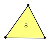
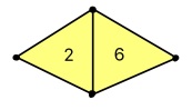
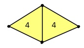
We can smooth out the intersection of two simple edges as . Similarly, we can smooth out the intersection of two triangles sharing a common edge as . This last equi-satisfiability is obtained from Lemma 4.1.
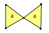
Smoothing out the intersection of two triangles sharing a common vertex results in a size hyperedge — . Smoothing at an edge-triangle pair with a common vertex yields .
We state without proof a general pattern for smoothing of hyperedges incident at a common vertex. For , we have —
4.3. Tucking edges
We now prove a series of reduction rules that allow deletion of degree or higher vertices, resulting in graphs with fewer edges. Visually, these operations look like tucking-in of an extended fin of the graph.
Tucking-in at an edge-hyperedge intersection incident at a common edge yields . This last equi-satisfiability follows from Lemma 4.1.
Degree intersections have reduction rules for the following cases —
-
(1)
A hyperedge with an edge incident on two of its three sides, i.e. .
-
(2)
A hyperedge of multiplicity , with an edge incident on one of its sides, i.e. .
-
(3)
A hyperedge with an edge of multiplicity two incident on one of its sides, i.e. .
For instance 1, we get —
For instance 2, we get —
Applying the graph-satisfiability map, yields —
4.4. Opening a triple-intersection vertex
We can replace a three-hyperedge intersection incident on a common vertex with three simple edges on the boundary. The proof of this reduction rule is as follows —
5. Satisfiability of mixed hypergraphs
In this section we provide a list of known totally satisfiable and unsatisfiable mixed-hypergraphs i.e. hypergraphs which have edges of size , or . List of candidate hypergraphs are generated programmatically using SageMath’s nauty package [4], which has various tools for generating canonically-labeled, non-isomorphic graphs with certain properties.
We list below several methods by which the satisfiability of a graph may be checked using our graphsat package —
-
(1)
If a graph is finite and small (fewer than 6 hyperedges), we can sat-check it by passing it to a graph satchecker. Such a satchecker can be found in the mhgraph_pysat_satcheck function in the sat.py module.
-
(2)
If a graph is finite but not too small (7 to 20 hyperedges), we can decompose it using local rewriting at the min-degree vertex. For this, we use the decompose function found in the graph_rewrite.py module.
-
(3)
If a graph is finite and big (20+ hyperedges), then we can reduce it to a smaller graph by passing it to the make_tree function in the operations.py module.
-
(4)
Lastly, if a graph is infinite, we have to work out its satisfiability status manually using reduction rules. Reduction rules themselves can be generated by the local_rewrite function in the graph_rewrite.py module.
Figure 1 shows a selection of unsatisfiable hypergraphs up to vertex size . A larger list can be found in the Appendix C.


5.1. Minimality of unsatisfiable hypergraphs
In the case of multi-graphs, we showed in [2] that satisfiability is invariant under homeomorphisms. We could then define a minimal unsatisfiable multi-graph to be one which is unsatisfiable, with every proper topological minor being totally satisfiable.
In the case of multi-hypergraphs, we have instead a list of reduction rules. The reduction rules make it harder to define minimality due to several reasons —
-
(1)
Given a list of reduction rule, it is a computationally expensive to check if any of these rules apply to a given graph.
-
(2)
For most reduction rules, the right side (which is what we obtain after rewriting) is not a single graph — it is instead a union of graphs. This means that any notion of minimality for hypergraphs must incorporate the effect of rewriting as a union of graphs instead of a single graph.
-
(3)
Our list of reduction rules is not complete. We may find more reduction rules by rewriting at higher degree vertices and carrying out longer computations. Each additional reduction rule could make the minimality criterion stricter and would shrink the size of any minimal set of unsatisfiable hypergraphs.
-
(4)
Uniqueness of the minimal set of unsatisfiable hypergraphs is not guaranteed owing to the complexity of the reduction rules.
5.2. Computational logistics
In this section we discuss the logistical setup used for carrying out all the calculations in this paper, along with a mention of the challenges posed by continuing these computations on bigger graphs in the face of exponentially more cases that need checking.
A computational procedure for finding all unsatisfiable looped-multi-hypergraphs can be carried out as follows —
- Step 1.:
-
Start with all looped-multi-hypergraphs sorted from smallest to largest. This can be done by calling nauty from inside SageMath. We use nauty to generate all graphs with the following properties inside a specified vertex range —
-
•:
the graph must be connected.
-
•:
total number of vertices must lie within specified range.
-
•:
edge sizes can be 1 (loops), 2 (simple edges), or 3 (hyperedges).
-
•:
we disallow edges of size 4 or higher in order to keep the computational task tractable.
-
•:
we specify that the minimum vertex degree of the graph should be 2 (since leaf vertices are known to be reducible).
-
•:
we allow an edge of size to only have multiplicity less than .
-
•:
- Step 2.:
-
Pick a graph and apply all known reduction rules to it.
- Step 3.:
-
Sat-check the irreducible part of the graph left over from Step 2 using brute-force strategy.
- Step 4.:
-
If totally satisfiable, then pick the next graph and go back to Step 2.
- Step 5.:
-
If unsatisfiable, then add the irreducible part to the list of known “minimal criminals”.
While this procedure allows us to search for small unsatisfiable graphs, it is clear that we have to contend with an exponential blowup in the number of graphs as well as an exponential blowup in the number of Cnfs that need to be sat-checked as we keep increasing the vertex count. Table 2 tabulates the number of graphs for different vertex ranges.
| Number of connected simple graphs with less than 7 vertices | 143 |
| Number of minimal unsatisfiable irreducible simple graphs | 4 |
| Number of connected looped-multi-hypergraphs with less than 6 vertices | 10080 |
| Number of minimal unsatisfiable irreducible L-M-H-graphs | 202 |
| Number of connected looped-multi-hypergraphs with less than 7 vertices | 48,364,386 |
| Number of minimal unsatisfiable irreducible L-M-H-graphs | unknown |
6. Satisfiability of triangulations
In this section we check a list of common/standard hypergraphs having edges of size exactly . These hypergraphs can be drawn as triangulations of various surfaces and are thus of interest when viewing GraphSAT from a topological point of view. We present computationally obtained satisfiability and unsatisfiability results. The choice of structures we study here is less systematic and more driven by ease of calculation.
6.1. Thickening of graph edges
We outline below a method to create triangulations starting with simple graphs, such that the satisfiability status in going from the simple graph to the triangulation remains unchanged.
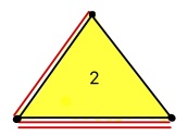
The process involves a local rewrite of every simple edge in a graph with the hyperedges , where and are new vertices not previously appearing in the graph.
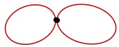
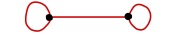
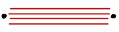
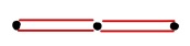
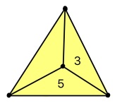
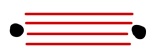
For example, since is an unsatisfiable graph, we can thicken all its edges into hyperedges to form the triangulation
This thickening process is shown in Figure 2.
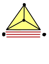

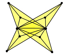
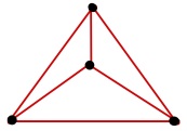
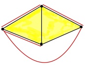
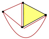
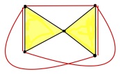
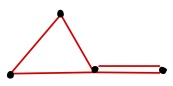
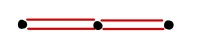
Similarly, thickening of the unsatisfiable graph results in the unsatisfiable triangulation shown in Figure 3. This triangulation is planar and can therefore be embedded in any surface. Thus, every surface has an unsatisfiable triangulation.
We also note that not all unsatisfiable triangulations are thickenings of unsatisfiable simple graphs. To prove that graph satisfiability is invariant under thickening of edges, we observe the following —
These reduction rules can be applied only because does not have any edges incident on vertices and since there vertices are newly introduced by the thickening process.
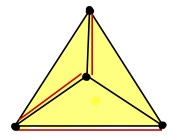
6.2. Tetrahedron and prisms
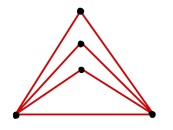
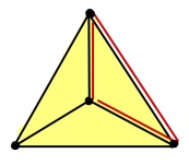
The tetrahedron’s wire-frame structure, i.e. its edges form the graph , a known unsatisfiable graph. The faces form the triangulation . Using the reduction rule from §4.4 gives
| Tetrahedron | |||
Thus the tetrahedron is totally satisfiable.
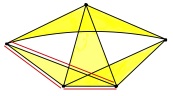
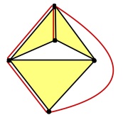
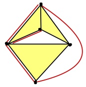
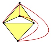
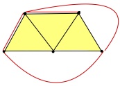
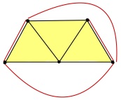
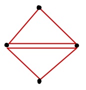
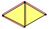
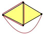
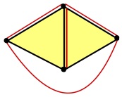
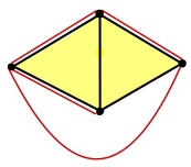
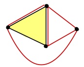
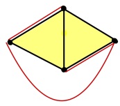
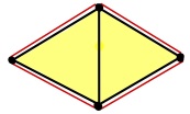
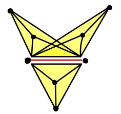
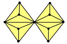
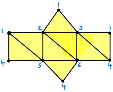
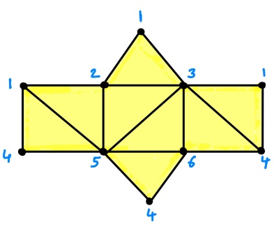
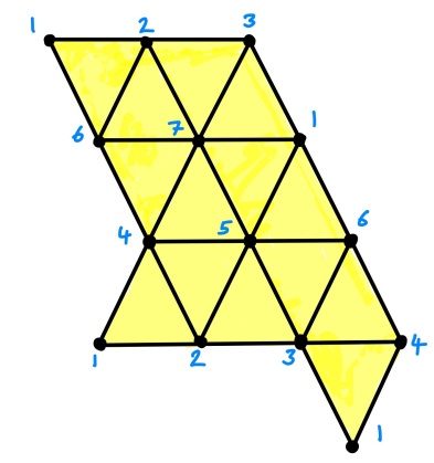
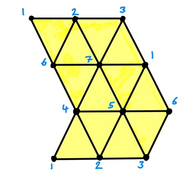
On the other hand the triangular prism has two possible minimal triangulations —
-
(1)
The symmetric triangulation, given by
-
(2)
The asymmetric triangulation, given by
These triangulations are shown in Figure 4. Passing them to the decompose function from the graph_rewite module tells us that both triangulations are totally satisfiable.
Output:
(1, 2, 3),(1, 2, 5),(1, 3, 4),(1, 4, 5),(2, 3, 6),(2, 5, 6),(3, 4, 6),(4, 5, 6)
    is SAT
(1, 2, 3),(1, 2, 5),(1, 3, 6),(1, 4, 5),(1, 4, 6),(2, 3, 6),(2, 5, 6),(4, 5, 6)
    is SAT
6.3. Triangulation of a Möbius strip
A Möbius strip can be triangulated as
(also shown in Figure 5). Using graph_rewrite.decompose, we conclude that this triangulation is totally satisfiable.
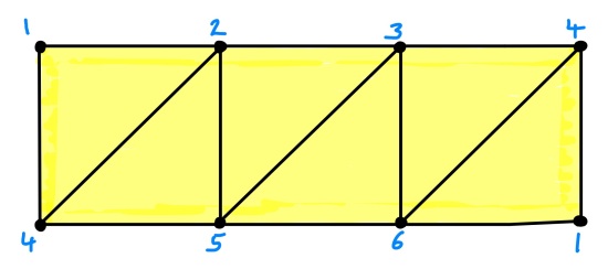
Output:
(1, 2, 4),(1, 4, 6),(2, 3, 5),(2, 4, 5),(3, 4, 6),(3, 5, 6) is SAT
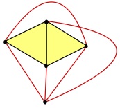
6.4. Minimal triangulation of the real projective plane
The minimal triangulation of has six vertices and is
unique up to relabeling of vertices. This triangulation is a classic result
and is often referred to in literature as . It can be
written as
, and is shown in Figure
6. Using graph_rewrite.decompose, we conclude that this
triangulation is totally satisfiable.
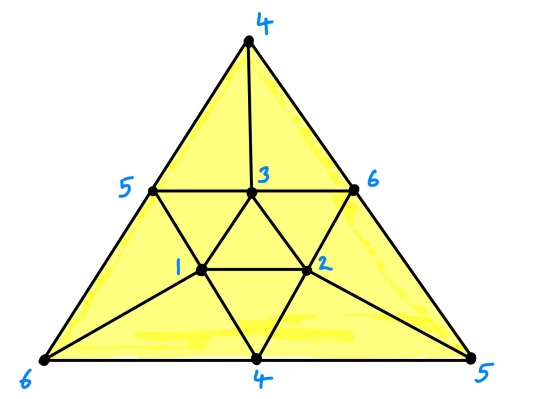
Output:
(1, 2, 3),(3, 2, 6),(4, 6, 1),(4, 1, 2),(5, 2, 6),(5, 6, 1),(1, 5, 3),
    (3, 6, 4),(4, 2, 5),(5, 3, 4) is SAT
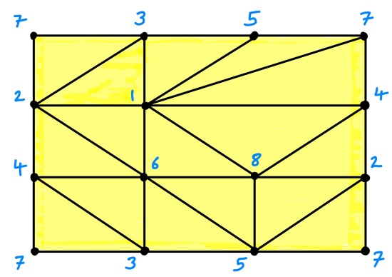
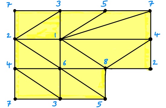
6.5. Minimal triangulation of a Klein bottle
A Klein bottle has six distinct -vertex triangulations [1]. These triangulations all contain distinct hyperedges and have a minimum vertex degree of . These large numbers make it difficult to determine the satisfiability status of these triangulations without committing to significant computational resources.
Of the six distinct triangulations, we checked but one — the “242
triangulation”, given by the faces
.
Passing it to graph_rewrite.decompose and waiting for several hours of computations results in the discovery that the configuration is unsatisfiable. In fact, it is unsatisfiable even if we remove the subgraph!
The triangulation and its unsatisfiable subgraph are shown in Figure 7 for reference.
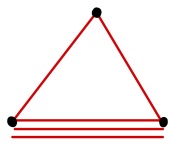
6.6. Minimal triangulation of a torus
The torus can be minimally triangulated [5] as —
.
This triangulation is shown in Figure 8 and is found to be
unsatisfiable by the
graph_rewrite.decompose function. In fact, it is unsatisfiable even if we
remove the subgraph.
7. Satisfiability of infinite graphs
We recall from §2.5 that is an arbitrary countable set, edges are nonempty sets of vertices, and graphs are nonempty multisets of edges. This definition does not exclude edges or graphs from being of countably infinite size. A graph with infinite edges, or edges of infinite size is an infinite graph.
We note that Cnfs, in a similar vein, can also be infinite. Infinite Cnfs either have infinitely many clauses, or have clauses of infinite size.
The notions of assignment, satisfiability, unsatisfiability — all carry over to infinite graphs and infinite Cnfs. The only notions that do not carry over are the questions of computational complexity since we cannot talk of program run-time for infinite instances of GraphSAT.
7.1. Infinitely many disconnected loops
The graph is a graph made of countably infinite disconnected self-loops. This graph is totally satisfiable because every connected component of it is.
7.2. Uniform infinite trees
For examples of totally satisfiable infinite graphs that are connected, we consider a family of tree graphs. For positive integer , let denote an infinite tree graph with each vertex being connected to exactly different vertices via edges of size . These are also sometimes referred to in the literature as infinite trees of uniform degree .
Each is in fact totally satisfiable since we proved in [2] that every tree is totally satisfiable and since the proof did not depend on the finiteness of the graph, the theorem still hold for infinite graphs .
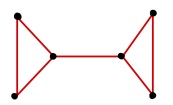
Another intuitive way to see that , for example, is totally satisfiable is that (at the level of Cnfs) each vertex can be used to satisfy its adjacent clause (see Figure 9). This results in a chain of assignments and each clause is satisfied in a style reminiscent of Hilbert’s famous infinite hotel.
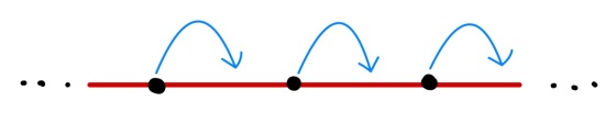
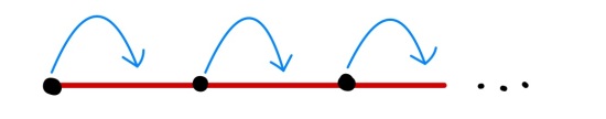
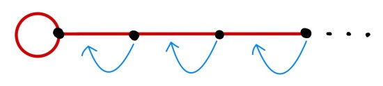
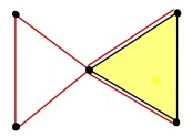
7.3. Infinite ray graph
Proof by demonstrating a vertex assignment also for other infinite graphs. We should keep in mind that a valid vertex assignment can only help us remove a single adjacent edge (or hyperedge) per vertex. Also, the existence of a vertex assignment implies that the graph in question is totally satisfiable, but its nonexistence does not prove that the graph is unsatisfiable.
We use this technique to argue that the infinite ray graph with a looped tail (see Figure 9) is totally satisfiable. At the level of Cnfs, we can see that the tail vertex can be used to satisfy the loop. The vertex next to the loop satisfies the last edge, the vertex after that satisfies that last-but-one edge, and so on. This assignment is shown in the figure using arrows. This proves that the infinite ray as well as the infinite ray with looped tail are both totally satisfiable graphs.
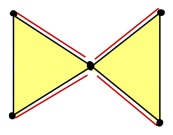
7.4. Bi-infinite strip
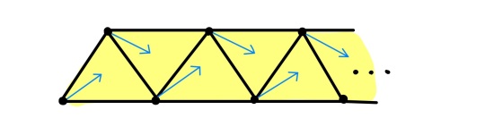
We next consider a thickened version of made of hyperedges, as shown in Figure 10. We call this is bi-infinite strip and claim that it is totally satisfiable. The assignment that satisfies a given Cnf in this graph can be derived by using the arrows shown in the figure. Similarly, the mono-infinite strip shown in Figure 10 is also totally satisfiable by the vertex assignment shown in the figure.
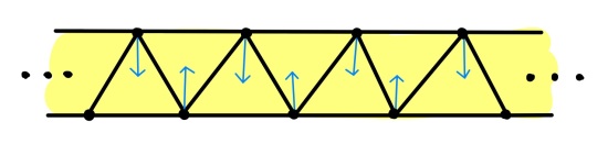
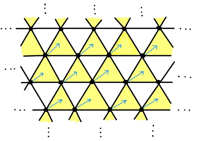
7.5. Plane tiling with missing alternate tiles
Lastly, we consider the tiling of the plane with alternate triangles and holes as shown in Figure 10. This triangulation can be satisfied by the vertex assignment shown in the same figure.
7.6. Compactness theorem and infinite GraphSAT
A graph is totally satisfiable if and only if every Cnf in it is satisfiable. The condition for every Cnf being satisfiable can itself be translated into a large Cnf if we allow the introduction of new variables.
For example, consider the single-edge graph . There is a set of Cnfs in the set , and by relabeling the vertices, we can write . We call this translation map from Graphs to Cnfs (short for translation).
We use this map to change the total-satisfiability question of a graph from a universal quantification over all Cnfs in to an existential quantification over all truth-assignments for the Cnf . This change to existential quantification allows us to apply the Compactness Theorem.
In mathematical logic, the Compactness Theorem states that a set of first-order sentences has a model if and only if every finite subset of it has a model. In the context of GraphSAT, this means that an infinite graph is totally satisfiable if and only if every finite subgraph of it is totally satisfiable. This means we can always restrict out attention to studying only finite graphs. It also means that any unsatisfiable infinite graph must have an unsatisfiable finite subgraph.
8. Conclusion and future directions
An outcome of this work is the creation of a new graph decision problem — GraphSAT. In [2] we showed that GraphSAT is in complexity class P and has a finite obstruction set containing four simple graphs [2]. The natural next step of exploring GraphSAT gave rise to the local graph rewriting theorem (Theorem 3.5), which leveraged the fact that taking a union over all possible vertex-assignments preserves the satisfiability status of a graph. Using this theorem, we were able to generate a list of graph reduction rules and an incomplete list of obstructions to satisfiability of multi-hypergraphs.
An incomplete list of known unsatisfiable looped-multi-hypergraphs (pictured in Figure 1 and listed in Appendix C.
8.1. Future directions
We showed that the complexity class of 2GraphSAT is P while the complexity class for 3GraphSAT is not known. Moreover, the effect of local graph rewriting on 3GraphSAT’s complexity class is not known. Hence a key research question that arises is whether local rewriting preserves complexity, and whether it makes 3GraphSAT easier in practice.
We have an incomplete list of unsatisfiable looped-multi-hypergraphs. Questions that arise within this context are — whether the number of essential sat-invariant graph reduction rules is finite? Even if the reduction rules are not finite, are they implementable in polynomial-time. Even if they are not implementable in polynomial time, it is possible that there is a polynomial-time check for demonstrating that none of the reduction rules apply to a given graph.
It is also not known if the number of minimal unsatisfiable graphs under these reduction rules is finite. So far we have found more than 200 distinct unsatisfiable and irreducible looped-multi-hypergraphs with less than 7 vertices. If the complete list is infinite, it would imply that 3GraphSAT is not in complexity class P.
If 3GraphSAT is in P, this would give us an easy P-time heuristic check for 3sat, simplifying some 3sat cases, while not directly affecting the complexity class of 3sat.
Let denote the complete -uniform hypergraph on vertices. To construct , we can start with vertices and connect all combinations with a hyperedge of size . We can also think of this as the -skeleton of a -simplex.
The hypergraph ’s satisfiability status is interesting because it combines the extreme of having all possible hyperedges connected (which can force unsatisfiability) with the extreme of each hyperedge being incident on a large number of vertices (which can force satisfiability).
For example, we know that is , i.e. the complete simple graph on vertices and is known to be totally satisfiable. On the other hand, the graph is is known to be totally satisfiable. Table 3 summarizes the known satisfiability statuses of various graphs. As seen in the table, the satisfiability-status of and are not known.
| b = 1 | b = 2 | b = 3 | b = 4 | b = 5 | b = 6 | b = 7 | ||
|---|---|---|---|---|---|---|---|---|
| a = 1 | sat | sat | sat | sat | sat | sat | sat | |
| a = 2 | - | sat | sat | unsat | unsat | unsat | unsat | |
| a = 3 | - | - | sat | sat | unsat | unsat | unsat | |
| a = 4 | - | - | - | sat | sat | sat | unknown | |
| a = 5 | - | - | - | - | sat | sat | unknown | |
| a = 6 | - | - | - | - | - | sat | sat | |
| a = 7 | - | - | - | - | - | - | sat | |
| - | - | - | - | - | - | - |
The generalized rule for triangular hyperedges meeting at a common free vertex is not known. We do know the reduction rule only for —
Reduction rules for yield massive data-tables of resulting Cnfs, which we have so far been unable to group into a convenient set of graphs.
Appendix A Operator and notation summary
All operators defined in §2 are summarized in Table 4. These operators are written in increasing order of binding-tightness. The order of binding-tightness can be used to disambiguate expressions when multiple operators are used at the same time.
| Operator | Context | Meaning | Remarks |
|---|---|---|---|
| Invisible glue | between literals | boolean disjunction | binds tighter than all other operators |
| , | between clauses or Cnfs | boolean conjunction | also written as |
| acts on literals | unary negation on literals | also written as | |
| action of assignment on Cnf | in §2.3 | ||
| between two Cnfs | equi-satisfiable Cnfs | equivalence relation | |
| Invisible glue | between vertices | adjacency of vertices | |
| superscript for a (hyper)edge | edge-multiplicity | ||
| , | between edges, or graphs | graph union | also called the adjacency of edges |
| between two sets of Cnfs | disjunction in §2.5.4 | ||
| between two sets of Cnfs | conjunction in §2.5.4 | ||
| action of vertex on a set of Cnfs | assignment in §3.1 | ||
| between two graphs | subgraph relation | ||
| between two graphs | shaved version | ||
| between two sets of Cnfs | equi-satisfiable graphs/sets | binds looser than all other operators |
Appendix B Standard graph disjunctions
Here we list tables of standard graph disjunctions that one may encountered when carrying out local graph rewriting calculations. These tables are all generated using the graph_or function in the operations.py module from our graphsat Python package. In §4 we use these disjunction results to derive graph reduction rules — global rewrites that do not affect the satisfiability of a graph. In §5.1, we describe an ongoing effort to describe the criterion for hypergraph minimality taking into account a growing list of graph reduction rules.
The first two tables list graph disjunctions that can be written exactly as a union of graphs; the third table lists graph disjunctions that can only be listed as a subset-superset pair.
| Subset | Superset | |||||
|---|---|---|---|---|---|---|
| () | ||||||
| () | ||||||
| () | ||||||
| () | ||||||
| () | ||||||
| () | ||||||
| () | ||||||
| ) | ||||||
| ) | ||||||
The above tables show that the possible graph disjunctions grow quickly with the edges participating in the disjunction. This is why we stop at a maximum of three edges. For calculating the graph disjunction of more edges, we can always use the graph_or function from the operations module on each individual disjunction.
Appendix C List of known unsatisfiable graphs
Presented below is a list of known unsatisfiable hypergraphs. This list was generated using SageMath’s nauty module and then filtering for unsatisfiable graphs.
 1  (1)
 2  (1), (2), (1,2)
 3  (1,2), (1,3), (1,4), (2,3), (2,4), (3,4)
 4  (1,2), (1,3), (2,3), (1,2,3), (1,2,4), (1,2,5), (3,4,5)
 5  (1,2), (1,3), (1,4), (2,3), (2,4), (1,2,5), (3,4,5)
 6  (1,2), (1,3), (1,4), (2,3), (2,4), (1,3,4)
 7  (1,2), (1,3), (1,4), (2,3), (2,4), (1,3,5), (2,4,5)
 8  (1,2), (1,4), (1,2,4)
 9  (1,2), (1,3), (1,4), (2,3), (1,2,4), (1,3,4)
10  (1,2), (1,3), (1,4), (2,3), (1,2,4), (1,4,5), (2,3,5)
11  (1,2), (1,3), (1,4), (2,3), (1,2,4), (1,3,5), (2,4,5)
12  (1,2), (1,3), (1,4), (2,3), (1,2,4), (2,3,4)
13  (1,2), (1,3), (1,4), (2,3), (1,2,4), (1,2,5), (3,4,5)
14  (1,2), (1,3), (1,4), (2,3), (1,2,5), (1,4,5), (3,4,5)
15  (1,2), (1,3), (1,4), (2,3), (1,4,5), (2,3,5), (2,4,5)
16  (1,2), (1,3), (1,4), (2,3), (1,4,5), (2,4,5), (3,4,5)
17  (1), (1,3)
18  (1,2), (1,4), (1,2,4)
19  (1,2), (1,3), (1,4), (2,3), (2,3,4)
20  (1,2), (1,3), (2,3)
21  (1,2), (1,4), (1,5), (1,4,5), (2,4,5)
22  (1,2), (1,3), (1,4), (1,5), (2,3), (2,4,5), (3,4,5)
23  (1,2), (1,3), (2,4), (1,2,4), (2,3,4)
24  (1,2), (1,3), (1,5), (2,4), (3,5), (2,3,4), (2,4,5)
25  (1,2), (1,3), (2,4), (1,2,3), (1,2,4), (1,3,4)
26  (1), (1,3), (1,5), (1,3,5), (3,4,5)
27  (1,2), (1,3), (1,5), (2,4), (1,2,4), (2,3,5), (3,4,5)
28  (1), (1,3), (1,3,4)
29  (1,2), (1,3), (2,4), (1,2,4), (2,3,4), (1,3,4)
30  (1,2), (1,3), (2,4), (1,3,4), (2,3,4)
31  (1,2), (1,3), (2,4), (3,4), (1,2,3), (1,2,4)
32  (1,2), (1,3), (2,4), (3,4), (1,2,5), (1,3,4), (3,4,5)
33  (1,2), (1,3), (2,4), (3,4), (1,2,4), (1,4,5), (2,3,5)
34  (1), (1,3), (3,4)
35  (1,2), (1,3), (1,5), (2,4), (3,4), (1,2,5), (3,4,5)
36  (1,2), (1,3), (2,4), (1,2,3), (1,2,4), (1,3,5), (2,4,5)
37  (1,2), (1,3), (2,4), (1,2,3), (1,2,4), (1,4,5), (2,3,5)
38  (1,2), (1,3), (2,4), (1,2,3), (1,2,4), (1,2,5), (3,4,5)
39  (1,2), (1,3), (2,4), (1,2,3), (1,2,5), (2,4,5), (3,4,5)
40  (1,2), (1,3), (2,4), (1,2,3), (1,4,5), (2,3,4), (2,3,5)
41  (1,2), (1,3), (2,3), (2,4), (3,5), (4,5), (1,4,5)
42  (1,2), (1,3), (2,4), (3,5), (4,5), (1,2,3), (1,4,5)
43  (2), (3,5)
44  (1,2), (1,3), (2,4), (3,5), (4,5), (1,2,5), (1,3,4)
45  (1,2), (1,3), (2,4), (4,5), (1,2,3), (1,3,5), (1,4,5)
46  (1,2), (1,3), (2,4), (4,5), (1,2,3), (1,3,5), (3,4,5)
47  (2), (2,3,5)
48  (1,2), (1,3), (2,4), (4,5), (1,2,3), (1,4,5), (2,3,5)
49  (1,2), (1,3), (2,4), (4,5), (1,2,3), (1,4,5), (3,4,5)
50  (2), (1,2), (1,3), (1,2,3), (1,3,5)
51  (1,2), (1,3), (2,4), (1,2,3), (1,3,5), (1,4,5), (2,4,5)
52  (1,2), (1,3), (2,4), (1,2,3), (1,4,5), (2,3,5), (2,4,5)
53  (1,2), (1,3), (2,4), (1,3,5), (1,4,5), (2,3,5), (2,4,5)
54  (1,2), (1,3), (2,4), (1,2,3), (1,3,5), (2,4,5), (3,4,5)
55  (1,2), (1,3), (4,5), (1,2,4), (1,2,5), (1,3,4), (1,3,5)
56  (1,2), (1,3), (4,5), (1,2,4), (1,3,5), (2,4,5), (3,4,5)
57  (1,2), (1,3), (4,5), (1,2,4), (1,3,4), (1,3,5), (2,4,5)
58  (1,2), (1,3), (4,5), (1,2,4), (1,3,4), (2,3,5), (2,4,5)
59  (1,2), (1,3), (4,5), (1,2,4), (1,3,4), (2,4,5), (3,4,5)
60  (1,2), (1,3), (2,4), (1,3,4), (2,3,4)
61  (1,2), (1,3), (2,4), (4,5), (1,2,5), (1,3,4), (3,4,5)
62  (1,2), (1,3), (2,4), (4,5), (1,2,5), (1,3,4), (1,3,5)
63  (1,2), (1,3), (2,4), (4,5), (1,3,4), (2,3,5), (3,4,5)
64  (1,2), (1,3), (2,4), (4,5), (1,2,5), (1,3,5), (2,3,4)
65  (1,2), (1,3), (2,4), (4,5), (1,3,5), (2,3,4), (3,4,5)
66  (1,2), (1,3), (2,4), (4,5), (1,2,4), (1,3,5), (2,3,5)
67  (1,2), (1,3), (2,4), (1,2,3), (1,4,5), (2,4,5), (3,4,5)
68  (1,2), (1,3), (2,4), (1,2,3), (1,3,5), (2,3,4), (2,4,5)
69  (1,2), (1,3), (2,4), (1,2,4), (1,2,5), (1,3,4), (3,4,5)
Appendix D Implementation of local graph rewriting
Below we include the docstring of the function, informing us what exactly the function does, followed by its implementation as a code-snippet. The implementation uses other functions defined in the package like operations.graph_or, compute_all_two_partitions_of_link, and mhgraph.rest. We will not detail each of these subsidiary functions here. We leave it instead to the interested reader to look at graphsat’s source code for more details.
Appendix E Implementation of graph disjunction
We present an implementation of graph disjunction as a Python function. This function can be found under the name graph_or in the operations.py module in our graphsat package. It computes the pairwise disjunction of the Cartesian product of two sets of Cnfs. Since the disjunction of two Cnfs is not a Cnf, we can bring it back into normal form using the function cnf_or_cnf which is outlined below as a helper function and is part of the prop.py module.
References
- [1] Cervone, D. P. Vertex-minimal simplicial immersions of the Klein bottle in three space. Geometriae Dedicata 50, 2 (Apr. 1994), 117–141. doi:10.1007/BF01265307.
- [2] Karve, V., and Hirani, A. N. The complete set of minimal simple graphs that support unsatisfiable 2-cnfs. Discrete Applied Mathematics 283 (2020), 123–132. doi:10.1016/j.dam.2019.12.017.
- [3] Karve, V., and Hirani, A. N. Github: vaibhavkarve/graphsat, Apr. 2021. doi:10.5281/zenodo.4662169.
- [4] McKay, B. D., and Piperno, A. Practical graph isomorphism, ii. Journal of Symbolic Computation 60 (2014), 94–112. doi:https://doi.org/10.1016/j.jsc.2013.09.003.
- [5] Möbius, A. F. Zur theorie der polyëder und der elementarverwandtschaft. Gesammelte werke 2 (1886), 513–560.
- [6] Robertson, N., and Seymour, P. Graph minors XX. Wagner’s conjecture. Journal of Combinatorial Theory, Series B 92, 2 (2004), 325 – 357. Special Issue Dedicated to Professor W.T. Tutte.