Can we imitate the principal investor’s behavior to learn option price?

Abstract

This paper presents a framework of imitating the principal investor’s behavior for optimal pricing and hedging options. We construct a non-deterministic Markov decision process for modeling stock price change driven by the principal investor’s decision making. However, low signal-to-noise ratio and instability that are inherent in equity markets pose challenges to determine the state transition (stock price change) after executing an action (the principal investor’s decision) as well as decide an action based on current state (spot price). In order to conquer these challenges, we resort to a Bayesian deep neural network for computing the predictive distribution of the state transition led by an action. Additionally, instead of exploring a state-action relationship to formulate a policy, we seek for an episode based visible-hidden state-action relationship to probabilistically imitate the principal investor’s successive decision making. Unlike conventional option pricing that employs analytical stochastic processes or utilizes time series analysis to model and sample underlying stock price movements, our algorithm simulates stock price paths by imitating the principal investor’s behavior which requires no preset probability distribution and fewer predetermined parameters. Eventually the optimal option price is learned by reinforcement learning to maximize the cumulative risk-adjusted return of a dynamically hedged portfolio over simulated price paths.

I Introduction

Modern quantitative finance employs the key idea of replicating a portfolio to bind financial derivative pricing to cross-sectional variation in underlying stock returns. Therefore, an effective way to model and simulate the distribution of future stock price movements is in demand and pivotal. Traditional models attempt to mirror the stock price movements as an analytical stochastic process or a combination of multiple random processes, such as the geometric Brownian motion in the Black–Scholes model [1], the compound Poisson process in the Merton jump diffusion model [2], the mean reverting square-root process combining two Wiener processes in Heston model [3], skewed Student’s t-distribution for the standardized residuals in $GARCH\left(p,q\right)$ [4]. However, framing the evolution of stock prices into stochastic processes is either too basic to cope with complexity or it relies on numerous undetermined parameters to be calibrated frequently.

This downside motivates us to develop a data-driven way to simulate underlying price movements to dispense with calibrating parameters by imitating the principal investor’s behavior and dynamically hedge portfolio over simulated price paths to learn option price. The Principal Investor (PI) refers to the collection of investors who have a leading influence on the stock market and the PI’s decision indicates the quantity of the capital that the PI chooses to invest in or sell out a particular underlying stock in the given time slot. We build our algorithm in three steps: 1. compute the predictive distribution of stock price change led by the PI’s decision, 2. imitate the PI’s successive decision making (the PI’s behavior) to simulate stock price paths, 3. learn option price to maximize the cumulative risk-adjusted return of a dynamically hedged portfolio over simulated price paths.

The interaction between the PI’s decision and stock price changes can be described by a non-deterministic Markov Decision Process (MDP) [5]. At each time step, MDP is in a state (spot price of the underlying stock) and the decision maker chooses an action (the PI’s decision) based on the current state. MDP then randomly moves into a new state with a probability that is influenced by the chosen action.

The predictive distribution of stock price change led by the PI’s decision instead of a fixed nonlinear relationship between stock price change and the PI’s decision is desired due to the reason that MDP is non-deterministic. For the purpose of deriving this predictive distribution from data, we resort to Bayesian Deep Neural Network (B-DNN) [6, 7, 8, 9] which introduces Bayesian statistics to Deep Neural Network (DNN) weights inference. Against a point estimate of DNN weights, B-DNN learns a probability distribution over the network weights. B-DNN predicts the probability distribution over price change induced by the PI’s decision through a two-stage process (1. Bayesian inference, 2. regression analysis). In the first stage, the distribution over B-DNN weights is inferred from the training dataset. Whereafter, a regression analysis is performed to model price change as a posterior predictive distribution which depends on the posterior distribution of DNN weights obtained from the first stage. Owing to the merit of DNN, the second step does away with a closed-form expression for non-linear multi-dimensional feature mapping. Instead, the regression analysis is built on a linear combination of basis vectors with few parameters to be pre-set. The numeric results based on real stock market data reveal that the PI’s decision and the stock price change are approximately positively correlated. We apply leader-follower type Keynesian beauty contest [10, 11] to explain the approximately positive correlation between the stock price change and the PI’s decision: a single retail investor easily believes that the instantaneous observation of the PI’s decision is the most investors’ concurrent decision to follow.

Leader-follower type Keynesian beauty contest discloses the behavior pattern of a single retail investor but not the PI’s strategy to make a decision that is also the last remaining piece of our MDP. In contrast to conventional MDP that associates a single type of factor (i.e., state) to the action selection by a policy function, we believe that the action selection depends on two types of factors (i.e., visible state and hidden state) and build a Visible-Hidden Markov Network to model the dependency of the PI’s decision making on visible factor and hidden factor. An algorithm is proposed to update the visible-hidden Markov network for best possibly fitting the visible state sequence and the observation sequence. Through the instrumentality of a trained visible-hidden Markov network for imitating the PI’s behavior from observations, we simulate the paths of the PI’s successive decision making and further transform them to stock price paths through Bayesian inference and regression analysis.

The final step to achieve our ultimate goal is designing an optimization criterion for pricing the option and a dynamic hedging algorithm that can efficiently take advantage of the cross-sectional information yielded by simulated price paths of the underlying stock. To this end, a self-financing portfolio is built to dynamically replicate the option price. The self-financing restriction raises a risk of exhausting cash for rebalancing the portfolio during the life of the option owing to a volatile price of the underlying stock. With the intention of minimizing this risk, the option price consists of a risk-free price and a risk-adjusted cost. The self-financing restriction also guarantees that the portfolio’s value change between adjacent time steps comes from the portfolio’s return. Thus, we are capable of exploiting reinforcement learning to maximize the cumulative risk-adjusted return for recursively learning the hedging position and pricing the option.

II Related Work

In the financial market, traditional Time Series Analysis (TSA) approaches play a dominant role to generate distribution for future stock prices. The linear TSA model, for example, Autoregressive Moving Average ($ARMA\left(p,q\right)$) forecasts the price through a linear regression that relates the targeted value to a linear combination of $p$ previous lag values, current residual error and $q$ past residual errors. $ARMA\left(p,q\right)$ is reliable only if the time series is stationary (in the sense of mean, variance, and covariance) without seasonality. $ARMA\left(p,q\right)$ is extended to cover the situation that the time series exhibits a trend and seasonal variation. ARMA Autoregressive Integrated Moving Average ($ARIMA\left(p,d,q\right)$) [12] introduces differencing to $ARMA\left(p,q\right)$ to eliminate the non-stationarity in the sense of mean (i.e. the trend). Seasonal ARIMA $\left(ARIMA\left(p,d,q\right)\times\left(P,D,Q\right)S\right)$ [13] incorporates additional seasonal differencing AR and MA terms into the non-seasonal ARIMA to deal with seasonal variation. The non-linear TSA models (Autoregressive Conditional Heteroskedasticity ($ARCH\left(p\right)$) / Generalized Autoregressive Conditional Heteroskedasticity ($GARCH\left(p,q\right)$) models) are employed to forecast the time series which is non-stationary in the sense of variance (time-varying volatility). $ARCH\left(p\right)$ models the variance at a time step as a linear combination of $p$ previous lag squared residual errors. $GARCH\left(p,q\right)$ model adds another linear combination of $q$ previous lag variance to $ARCH\left(p\right)$. The non-linear models have been improved in recent studies, for example, [14] works on fitting skewness to make distribution assumptions about the residuals as financial time series data often has a deviation from a normal distribution. In practice, the linear TSA model and the non-linear TSA model are commixed to generate the distribution for future stock prices. For instance, $ARMA\left(p,q\right)$ is used to forecast the mean and $GARCH\left(p,q\right)$ gives the volatility prediction.

Recently deep neural network-based approaches for stock price prediction have attracted much attention. [15, 16] propose to apply recurrent neural networks, such as Long short-term memory (LSTM) networks and gated recurrent unit (GRU) to financial time series predictions. Graph Neural Networks (GNN) are considered as an effective deep learning model for stock movement prediction in [17, 18]. In [19, 20], authors recommend Convolutional Neural Network (CNN) as a novel method for predicting stock price movements.

Our proposed approach generates the distribution of stock price by imitating the principal investor’s behavior based on B-DNN and visible-hidden Markov. Compared with TSA approaches, our approach does not require many pre-determined parameters and is not reliant on any preset probability distribution. As a counter example, we have to decide order $\left(p,q\right)$ through statistical tests and specify the distribution assumptions about the residuals before using $GARCH\left(p,q\right)$. In addition, our proposed approach generates the distribution of stock price instead of predicting the stock price as above listed recent deep neural network-based approaches are used for.

III Effect of the principal investor’s decision

As described in the introduction section, we are motivated to model the evolution of the underlying stock price by virtue of DNN and behavioral analysis, rather than analytically characterize stochastic processes in a traditional way. With this end in view, a non-deterministic MDP is designed to associate stock price evolution with the PI’s successive decision making. This section is on a quest for the impact of PI’s decision on stock price change.

We define PI as the aggregation of investors who are considered as the dominating force in the equity market. PI could be composed of large institutional investors or a sizable group of retail investors acting in concert. PI’s decision is concerned with the amount of money flowing into or out of a stock within a time slot. We approximately quantize PI’s decision as a signed number $d\in\varOmega_{d}$ in terms of the opening price $o\in\varOmega_{o}$, the highest price $h$, the lowest price $l$, the closing price $c\in\varOmega_{c}$, and the volume $v$:

$$d=\left(vh\frac{h-o}{h-l}\right)\mathrm{\textrm{sign}\left(\mathit{c-o}\right)}.$$ (1)

This representation allows the difference between the opening and closing prices to indicate the direction of the money flow. Moreover, the difference between the opening and highest prices becomes a primary determinant of the money flow volume. Through simple math deduction, this synthetic variable can be proved to have a monetary unit, and we consider it as USD in this paper.

The sample spaces $\varOmega_{d}$ and $\varOmega_{o}$ (or $\varOmega_{c}$) constitute respectively the MDP action space and state space. The price change functions as an indicator of the MDP state transition:

$$g=\frac{c}{o}-1$$ (2)

We presume that the price change is incompletely impacted by PI’s decision and partly random. This implies that the price change follows a probability distribution which is dependent on PI’s decision. We intend to use a data-driven regression method to determine this probability distribution and verify our presumption. For this aim, we resort to B-DNN [6, 7, 8, 9] which applies Bayesian statistics to DNN weights inference. By further merging B-DNN with Gaussian process [21, 22], the price change distribution is simplified as a gaussian distribution.

Given a dataset $\mathcal{\mathscr{D}}\coloneqq\left\{\left(d_{n},g_{n}\right)\right\}_{n=0}^{\mathrm{T}-1}$which contains pairs of quantized PI’s decision and the price change sampled from $\mathrm{T}$ consecutive time slots, we apply gradient ascent coupled with the dataset $\mathscr{D}$ to train a DNN. The DNN takes an input data $d_{n}$ and returns a predicted value $f_{\boldsymbol{\theta}}\left(d_{n}\right)\in\mathbb{R}$ to compare with the observed value $g_{n}$ for producing the empirical loss, where $\boldsymbol{\theta=}\left[\theta_{1},\ldots,\theta_{M}\right]^{T}$ signifies the DNN weights. The loss is defined in terms of the loss function $l\left(g_{n},f_{\boldsymbol{\theta}}\left(d_{n}\right)\right)$ and the $L2$ regularizer $\mathscr{\mathit{r}}\left(\boldsymbol{\theta}\right)$ with a regularization parameter $\lambda$:

$$\mathscr{L}\left(\boldsymbol{\theta},\mathscr{D}\right) =L\left(\boldsymbol{\theta},\mathscr{D}\right)+\mathscr{\mathit{r}}\left(\boldsymbol{\theta}\right)$$

$$=\sum_{n=0}^{\mathrm{T}-1}l\left(g_{n},f_{\boldsymbol{\theta}}\left(d_{n}\right)\right)+\frac{\lambda}{2}\boldsymbol{\theta}^{T}\boldsymbol{\theta}.$$ (3)

In contrast to fit a point estimate of DNN weights, B-DNN learns a distribution over the weights. We take advantage of this merit of B-DNN to infer the posterior distribution over the weights (Bayesian inference) and therefore derive a posterior predictive distribution which measures the distribution over price change induced by PI’s decision (Regression analysis).

In order to implement Bayesian inference on the weights, the loss is straightforwardly embedded in the posterior distribution over the weights via the exponential family form $P\left(\boldsymbol{\theta}\mid\boldsymbol{\mathscr{D}}\right)\coloneqq\frac{e^{\mathscr{-L}\left(\boldsymbol{\theta},\mathscr{D}\right)}}{\int e^{\mathscr{-L}\left(\boldsymbol{\theta},\mathscr{D}\right)}d\boldsymbol{\theta}}$. It implies both the likelihood and the prior also belong to the exponential family with the expression as $P\left(\mathscr{D}\mid\boldsymbol{\theta}\right)\coloneqq\frac{e^{-L\left(\boldsymbol{\theta},\mathscr{D}\right)}}{\int e^{-L\left(\boldsymbol{\theta},\mathscr{D}\right)}d\boldsymbol{\theta}}$ and $P\left(\boldsymbol{\theta}\right)\coloneqq\frac{e^{\mathit{-r}\left(\boldsymbol{\theta},\mathscr{D}\right)}}{\int e^{\mathit{-r}\left(\boldsymbol{\theta},\mathscr{D}\right)}d\boldsymbol{\theta}}$. In such a manner, the Maximum A Posteriori (MAP) estimation $\widehat{\boldsymbol{\theta}}=\underset{\boldsymbol{\theta}}{\arg\max}\,P\left(\boldsymbol{\theta}\mid\boldsymbol{\mathscr{D}}\right)$ is equivalent to minimize mean square error. However, the immediate MAP estimation is often computationally impractical.

Laplace approximation [23, 24, 25] provides a computationally feasible Bayesian inference on weights. The main idea is to approximate likelihood times prior with a Gaussian density function in respect that likelihood times prior is a well-behaved uni-modal function in $\mathcal{L}^{2}$ space. The posterior distribution over the weights is consequently derived to be the below Gaussian distribution (see derivation in Appendix A):

$$P\left(\mathrm{\boldsymbol{\theta}}|\mathcal{\mathscr{D}}\right)\approx\mathcal{N}\left(\boldsymbol{\theta}\mid\boldsymbol{\theta}^{*},\left[\nabla_{\boldsymbol{\theta\theta}}^{2}L\left(\boldsymbol{\theta}^{*},\mathscr{D}\right)+\lambda\mathbf{I}_{\mathit{M}}\right]^{-1}\right),$$ (4)

where $\boldsymbol{\theta}^{*}=\left[\theta_{1}^{*},\ldots,\theta_{M}^{*}\right]^{T}$ is the mode of $P\left(\mathscr{D}\mid\boldsymbol{\theta}\right)P\left(\boldsymbol{\theta}\right)$.

After obtaining the posterior over the weights, we then seek for the posterior predictive distribution over price change $P\left(g^{*}\mid d^{*},\mathscr{D}\right)$, where $d^{*}\in\mathbb{R}$ denotes a test sample of quantized PI’s decision and $g^{*}$ signifies the corresponding observation of the price change. The high dimensional projection and the nonlinear relationship between $d^{*}$ and $f_{\boldsymbol{\theta}^{*}}\left(d^{*}\right)$ impede to directly find $P\left(g^{*}\mid d^{*},\mathscr{D}\right)$ in closed form. In order to overcome this impediment, a new random variable $y$ which has a readily accessible posterior predictive distribution is constructed and can be linearly expressed in terms of $g^{*}$. As a result, $P\left(g^{*}\mid d^{*},\mathscr{D}\right)$ is inferred from the given posterior predictive distribution $P\left(y\mid d^{*},\mathscr{D}\right)$. As presented in [21], $y$ is possible to be designed as a linear combination of a Gaussian process and additive gaussian noise. Different from [21], we calculate the parameters of the Gaussian process (i.e., $m\left(d^{*}\right)$ in Equation (11) and $k\left(d^{*},d^{*}\right)$ in Equation (12)) based on $P\left(\mathrm{\boldsymbol{\theta}}|\mathcal{\mathscr{D}}\right)$ instead of $P\left(\mathrm{\boldsymbol{\theta}}|\mathcal{\mathscr{\mathscr{D}^{\prime}}}\right)$ where $\mathscr{D}^{\prime}\coloneqq\left\{\left(y_{n},c_{n}\right)\right\}_{n=0}^{\mathrm{T}-1}$ is a transformed dataset and $y_{n}$ is a sample of the constructed variable. In addition, we consider the residual ($\varepsilon$ in Equation (10)) as additive independent identically distributed (i.i.d) Gaussian noise rather than additionally bring in the second-order partial derivatives of the loss to represent noise.

The random variable $y$ is designed as the following combination of the standard linear regression model and the first order derivative of the loss function:

$$y=\boldsymbol{\phi}\left(d^{*}\right)^{T}\boldsymbol{\theta}+\nabla_{f_{\boldsymbol{\theta}^{*}}\left(d^{*}\right)}l\left(g^{*},f_{\boldsymbol{\theta}^{*}}\left(d^{*}\right)\right),$$ (5)

where DNN weights follow a prior distribution $\boldsymbol{\theta}\sim\mathcal{N}\left(\mathbf{0},\mathbf{K}_{\boldsymbol{\theta\theta}}\right)$ with the covariance matrix $\mathbf{K}_{\boldsymbol{\theta\theta}}=\lambda^{-1}\mathbf{I}_{\mathit{M}}$. And $\boldsymbol{\phi}\left(d^{*}\right)$ is a Jacobian matrix whose entries form a set of basis functions to project the input sample into $M$ dimensional feature space:

$$\boldsymbol{\phi}\left(d^{*}\right) =\nabla_{\boldsymbol{\theta}}f_{\boldsymbol{\theta}}\left(d^{*}\right)\mid_{\boldsymbol{\theta}=\boldsymbol{\theta}^{*}}$$

$$=\left[\begin{array}[]{c}\frac{\partial f_{\boldsymbol{\theta}}\left(d^{*}\right)}{\partial\theta_{1}}\mid{}_{\theta=\theta_{1}^{*}}\\ \vdots\\ \frac{\partial f_{\boldsymbol{\theta}}\left(d^{*}\right)}{\partial\theta_{M}}\mid_{\theta_{M}=\theta_{M}^{*}}\end{array}\right],$$ (9)

As the linear regression model is built on the feature space in Equation (9), it successfully leaves the difficulty of processing non-linear high-dimensional mapping back to DNN.

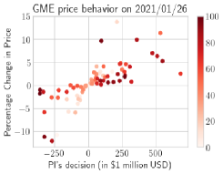
(a)

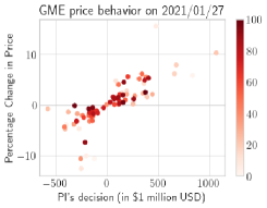
(b)

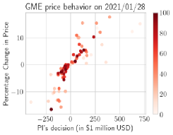
(c)

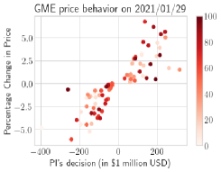
(d)

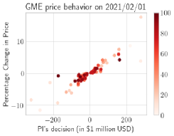
(e)

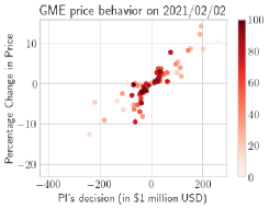
(f)

Figure 1: GME behavior observed in each 5-minute time slot from 09:35 to 16:00 during 6 consecutive trading days. Earlier time slots are with lighter shades.

For a quadratic loss function $l\left(g^{*},f_{\boldsymbol{\theta}^{*}}\left(d^{*}\right)\right)=\frac{1}{2}\left(g^{*}-f_{\boldsymbol{\theta}^{*}}\left(d^{*}\right)\right)^{2}$, the constructed random variable $y$ can be simplified in terms of $g^{*}$ from Equation (5):

$$y =\boldsymbol{\phi}\left(d^{*}\right)^{T}\boldsymbol{\theta}+\left(f_{\boldsymbol{\theta}^{*}}\left(d^{*}\right)-g^{*}\right)$$

$$=\varphi\left(d^{*}\right)+\varepsilon,$$ (10)

where $f_{\boldsymbol{\theta}^{*}}\left(d^{*}\right)-g^{*}$ is the residual that can be modeled as additive independent identically distributed Gaussian noise $\varepsilon\sim\mathcal{N}\left(0,\sigma^{2}\right)$. Gaussian process is an effective tool for describing a distribution over functions [22]. From the function-space view, the process $\varphi\left(d^{*}\right)$ is specified by a Gaussian process $\varphi\left(d^{*}\right)\sim\mathcal{GP}\left(m\left(d^{*}\right),k\left(d^{*},d^{*}\right)\right)$, where we calculate the mean function $m\left(d^{*}\right)$ and the covariance function $k\left(d^{*},d^{*}\right)$ based on the posterior distribution over the weights $P\left(\mathrm{\boldsymbol{\theta}}|\mathcal{\mathscr{D}}\right)$ obtained in Equation (4):

$$m\left(d^{*}\right) =\boldsymbol{\phi}\left(d^{*}\right)^{T}\mathbb{E}\left[\boldsymbol{\theta}\mid\mathscr{D}\right]$$

$$=\boldsymbol{\phi}\left(d^{*}\right)^{T}\boldsymbol{\theta}^{*},$$ (11)

$$k\left(d^{*},d^{*}\right) =\phi\left(d^{*}\right)^{T}\mathbb{E}\left[\boldsymbol{\theta\theta}^{T}\mid\mathscr{D}\right]\phi\left(d^{*}\right)$$

$$=\phi\left(d^{*}\right)^{T}\left[\nabla_{\boldsymbol{\theta\theta}}^{2}L\left(\boldsymbol{\theta}^{*},\mathscr{D}\right)+\lambda\mathbf{I}_{\mathit{M}}\right]^{-1}\phi\left(d^{*}\right).$$ (12)

Equation (10) exhibits that the random process $y$ is a linear combination of a Gaussian process and additive Gaussian noise. Therefore, the posterior predictive distribution of $y$ can be easily deduced from the statistical description of the Gaussian process and Gaussian noise as:

$$P(y\mid d^{*},\mathscr{D})=\mathcal{N}\left(\boldsymbol{\phi}\left(d^{*}\right)^{T}\boldsymbol{\theta}^{*},k\left(d^{*},d^{*}\right)+\sigma^{2}\right).$$ (13)

Since we always prefer to perform a prediction based on the DNN weights at the mode of the posterior $\boldsymbol{\theta}^{*}$ rather than any possible DNN weights, only the determinate realization $\boldsymbol{\phi}\left(d^{*}\right)^{T}\boldsymbol{\theta}^{*}$ should be extracted from the Gaussian process instead of the entire Gaussian process $\boldsymbol{\phi}\left(d^{*}\right)^{T}\boldsymbol{\theta}$ for calculating $g^{*}$. Thuswise $g^{*}$ is a linear combination of a random variable and a constant:

$$g^{*} =y-\boldsymbol{\phi}\left(d^{*}\right)^{T}\boldsymbol{\theta}^{*}+f_{\boldsymbol{\theta}^{*}}\left(d^{*}\right)$$

$$=y+C.$$ (14)

Consequently, the posterior predictive distribution over price change is derived from Equation (13) and (14):

$$P(g^{*}\mid d^{*},\mathscr{D})=\mathcal{N}\left(f_{\boldsymbol{\theta}^{*}}\left(d^{*}\right),k\left(d^{*},d^{*}\right)+\sigma^{2}\right).$$ (15)

The observation of the price change $g^{*}$ shares the same posterior predictive variance with $y$ owing to the fact that the predicted value $\boldsymbol{\phi}\left(d^{*}\right)^{T}\boldsymbol{\theta}^{*}$ is a determinate realization produced at the mode of the posterior $\boldsymbol{\theta}^{*}$ and the deduction of the predicted value from $y$ is incapable of eliminating the immanent uncertainty in the inference on weights and the residual. When we consider an input vector of test samples $\mathbf{d}^{*}$=$\left[d_{1}^{*},\ldots,d_{N}^{*}\right]^{T}$, Equation (15) turns into the below form:

$$P(g^{*}\mid\mathbf{d}^{*},\mathscr{D})=\mathcal{N}\left(f_{\boldsymbol{\theta}^{*}}\left(\mathbf{d}^{*}\right),diag\left(\mathit{k}\left(\mathbf{d}^{*},\mathbf{d}^{*}\right)+\sigma^{2}\mathbf{I}_{\mathit{N}}\right)\right).$$ (16)

During Jan. 26, 2021-Feb. 02, 2021, GameStop Corporation (GME) stock price swiftly rose and then fell with the unusually high price and volatility because a short squeeze was triggered by organized retail investors. We would like to explore the behavioral finance behind this event through our model. The intraday data for the 6 consecutive trading days is exercised to infer B-DNN coefficients and be referred to produce testing samples for validating regression analysis. Due to the unreachability, the pre/post-market data is not included even though some huge price fluctuations occurred in the pre/post-market sessions. We structure a dataset $\mathcal{D}$ as 77 samples in each of 6 episodes to accommodate the equity pricing data in the period from 09:35 to 16:00 for the 6 consecutive trading days. Each sample is a five-dimensional vector which enumerates open-high-low-close prices and volume observed in a 5-minute time slot. We discard the pricing data in the first time slot (i.e., 09:30 to 09:35) because the open price is subject to the pre-market trading and gaps up or down from the previous day’s close. Moreover, the volume in the first time slot is extremely high and influenced by the pre-market news. Based on Equation (1), (2) and dataset $\mathcal{D}$, we yield the training dataset $\mathcal{\mathscr{D}}_{i}\coloneqq\left\{\left(d_{n},g_{n}\right)\right\}_{n=0}^{\mathrm{T}_{i}-1}$ which contains the pairs of quantized PI’s decision and price change sampled from $\mathrm{T}_{i}$ consecutive time slots in the $i$th episode as illustrated in Figure 1. The samples are plotted in chronological order. The lighter shade indicates that the sample is taken in an earlier time slot.

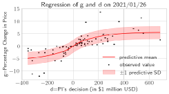
(a)

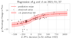
(b)

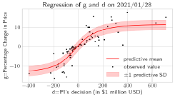
(c)

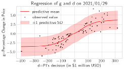
(d)

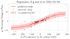
(e)

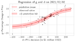
(f)

Figure 2: Regression with $\sigma=2.5$ and $\lambda=0.7$

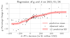
(a)

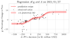
(b)

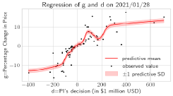
(c)

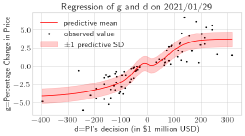
(d)

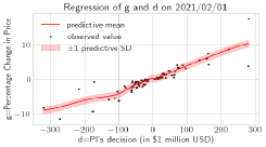
(e)

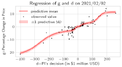
(f)

Figure 3: Regression with $\sigma=1$, $\lambda=0.1$

We first train B-DNN respectively on an episode basis with the training dataset $\mathcal{\mathscr{D}}_{i,i=1\ldots 6}$ to determine the posterior distribution over the weights and then work out the posterior predictive distribution over price change led by testing samples of quantized PI’s decision. The testing samples are produced to be evenly spaced over the interval between the largest and smallest training sample of quantized PI’s decision in each episode. There are two fine-tuned hyperparameters $\sigma$ and $\lambda$ for optimizing our model’s performance. Since $\sigma$ has a significant influence on posterior predictive variance as shown in Equation (15), the optimal value of $\sigma$ can be found out by the "68–95–99.7 rule". We carry out Bayesian inference and regression analysis with two sets of parameters ($\sigma=2.5$, $\lambda=0.7$, and $\sigma=1$, $\lambda=0.1$) and exhibits the results in turn by Figure 2 and Figure 3. It is observed that $\sigma=2.5$ offers a fitting posterior predictive variance to satisfy in principle the "68–95–99.7 rule", while $\sigma=1$ leads to a too small posterior predictive variance to match the actual data distribution. The experimental evaluation also demonstrates that the overfitting is effectively prevented by $\lambda$. As shown in Figure 2, the overfitting is fully suppressed by a relatively large regularization parameter $\lambda=0.7$. On the other hand, overfitting emerges when the regularization parameter decreases to a smaller value, for instance, $\lambda=0.1$ as illustrated in Figure 3. Furthermore, we can observe from the numeric results that the stock price change has an approximately positive correlation with quantized PI’s decision.

IV Inverse PI’s decision from visible and hidden states

The previous section presents a DNN-based approach to determine the state transition (i.e., price change) after executing an action (i.e., principal investor’s decision). We still wonder how an action is made and especially how to associate an action with the current state (i.e., open price). Answering this query equals the proffer of the last remaining piece of our MDP. This section will find out the underlying law to simulate PI’s successive decision making.

When we ground the numerical results on the real equities pricing data in the previous section, it is observed that higher quantized PI’s decision approximately leads to higher stock price change. This phenomenon can be theoretically explained by the Keynesian beauty contest [10, 11]. Keynesian beauty contest describes a beauty contest where voters win a prize for voting the most popular faces among all voters. Under such a rule of the contest, a voter tends to guess the other voters’ choices and match the choice of the majority based on his or her own guess. Keynes believed that the similar behavior pattern applies to the investors within the stock market. Most investors attempt to make the same decision that the majority do rather than build a decision on their own evaluation of fundamental profitability. However, it is very hard to guess another investor’s concurrent decision for a retail investor. For this reason, the stock market evolves into a leader-follower type Keynesian beauty contest where a single retail investor (i.e., follower) tends to follow the instantaneous observation of PI’s decision and thinks it as the most investors’ concurrent decision. The leader-follower type Keynesian beauty contest explains well the approximately positive correlation between PI’s decision and the stock price change. Nevertheless, PI’s decision making is still inadequate to be inferred from the leader-follower type Keynesian beauty contest.

We believe that two types of factors influence PI’s decision making: visible and hidden. The visible factor is observable, while the hidden factor is hard to be quantized or detected, for example, the impact of news on investors’ anticipation of the investment return and thus on their investment behavior.

The conventional MDP applies a policy function to map state space to action space. However, the policy function is not sufficient for mapping two state spaces to action space. In order to identify the dependency of PI’s decision making on visible factor and hidden factor, we build a visible-hidden Markov network as shown in Figure 4. The hidden factor is modeled by a random variable (i.e., hidden state) which changes through time and the visible factor is modeled by another random variable (i.e., visible state). The hidden state transits over time slots, and its transition is a Markov process. In the same time slot, the hidden state, the visible state, and the random variable representing PI’s decision (i.e., observation) are pairwise correlated. We design a chain for connecting these random variables to enable the calculation of the dependencies among them. This chain design differentiates the visible-hidden Markov network from hidden Markov models [26] which considers only two coinstantaneous components without the visible state. In each time slot, the hidden state is directly connected to the visible state and then indirectly chained to the observation via the visible state.

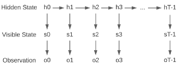
Figure 4: Visible-hidden Markov network

We specify the notations used in the visible-hidden Markov network below:

$\zeta=\left\{\zeta_{0},\zeta_{1},\ldots,\zeta_{J-1}\right\}$: hidden state sample space,

$\nu=\left\{\nu{}_{0},\nu_{1},\ldots,\nu_{K-1}\right\}$: visible state sample space,

$\omega=\left\{\omega_{0},\omega_{1},\ldots,\omega_{L-1}\right\}$: observation sample space,

$Z=\left\{z_{0},z_{1},\ldots,z_{J-1}\right\}$: initial hidden state distribution,

$\mathbf{A}=\left\{a_{ij}\right\}\in\mathbb{R}^{J\times J}$: hidden state transition matrix,

$a_{ij}=P\left\{\mathrm{hidden\;state}\;\zeta_{j}\;\mathrm{at}\;t+1\mid\mathrm{hidden\;state}\;\zeta_{i}\;\mathrm{at}\;t\right\}$,

$\mathbf{B}=\left\{b_{i}\left(k\right)\right\}\in\mathbb{R}^{J\times K}$: visible state probability matrix,

$b_{i}\left(k\right)=P\left\{\mathrm{visible\;state}\;v_{k}\;\mathrm{at}\;t\mid\mathrm{hidden\;state}\;\zeta_{i}\;\mathrm{at}\;t\right\}$,

$\mathbf{C}=\left\{c_{k}\left(l\right)\right\}\in\mathbb{R}^{K\times L}$: observation probability matrix,

$c_{k}\left(l\right)=P\left\{\mathrm{observation\;}o_{l}\;\mathrm{at}\;t\mid\mathrm{visible\;state}\;v_{k}\;\mathrm{at}\;t\right\}$,

$H=\left\{h_{0},h_{1},\ldots,h_{\mathrm{T}-1}\right\}$: hidden state sequence,

$S=\left\{s_{0},s_{1},\ldots,s_{\mathrm{T}-1}\right\}$: visible state sequence,

$O=\left\{o_{0},o_{1},\ldots,o_{\mathrm{T}-1}\right\}$: observation sequence,

$\Gamma=\left\{\mathbf{A},\mathbf{B},\mathbf{C},Z\right\}$: Visible-hidden Markov network.

In our scenario, the hidden state indicates bullish or bearish news received just before a time slot, so the hidden state sample space $\zeta$ is with a size of 2. The visible state and the observation chained to the same hidden state respectively represent the opening price and quantized PI’s decision in the same time slot influenced by the just acquired market information. The visible state sample space $\nu$ and the observation sample space $\omega$ are finite and discrete compared with the continuous sample space of the opening price and quantized PI’s decision. For this reason, we borrow the concept of the quantization in digital signal processing to map values from the sample space of the opening price and quantized PI’s decision to $\nu$ and $\omega$:

$$\bar{s}=\lfloor\frac{s}{\frac{s_{max}-s_{min}}{\mathsf{Q}}}\rfloor,$$ (17)

where $\left\lfloor\right\rfloor$ is the floor function. $s$ stands for a sample value of the opening price or quantized PI’s decision. $s_{max}$ and $s_{min}$ mark respectively the upper and lower limits of the sample space of the opening price or quantized PI’s decision. $\mathsf{Q}$ denotes the size of $\nu$ or $\omega$ which is $K$ or $L$. $\bar{s}$ is mapped from $s$ to constitute $\nu$ or $\omega$.

The hidden state is initialized from a distribution $Z$ and transits based on a transition probability matrix $\mathbf{A}$. In the same time slot, the visible state is related to the hidden state by a probability matrix $\mathbf{B}$ and the observation is associated with the visible state by another probability matrix $\mathbf{C}$ to form a chain. Our objective is to find $\Gamma=\left\{\mathbf{A},\mathbf{B},\mathbf{C},Z\right\}$ which best possible fits the visible state sequence $S$ and the observation sequence $O$. To this end, an algorithm is proposed to modulate $\Gamma$ by iteratively increasing $P\left(S,O\mid\Gamma\right)$:

Step 1: Initialize $\Gamma$ and set $P\left(S,O\mid\Gamma\right)=0$.

Step 2: Calculate the conditional joint probability function $\alpha_{t}\left(i\right)$, $\beta_{t}\left(i\right)$,$\gamma_{t}\left(i,j\right)$ and the conditional probability function $\gamma_{t}\left(i\right)$:

$$\alpha_{t=0}\left(i\right) =P\left(\mathcal{\mathit{s}}_{0},\mathcal{\mathit{o}}_{0},h_{0}=\zeta_{i}|\Gamma\right)$$

$$=z_{i}b_{i}\left(s_{0}\right)c_{s_{0}}\left(o_{0}\right),$$ (18)

$$\alpha_{t>0}\left(i\right) =P\left(\mathcal{\mathit{s}}_{0},\mathcal{\mathit{s}}_{1},\ldots,\mathcal{\mathit{s}}_{t},\mathcal{\mathit{o}}_{0},\mathcal{\mathit{o}}_{1},\ldots,o_{t},h_{t}=\zeta_{i}|\Gamma\right)$$

$$=\sum_{j=0}^{K-1}\alpha_{t-1}\left(j\right)a_{ji}b_{i}\left(s_{t}\right)c_{s_{t}}\left(o_{t}\right),$$ (19)

$$\beta_{t=\mathrm{T}-1}\left(i\right)=P\left(\mathcal{\mathit{s}}_{\mathrm{T}-1},\mathcal{\mathit{o}}_{\mathrm{T}-1}|h_{\mathrm{T}-1}=\zeta_{i},\Gamma\right)=1,$$ (20)

$$\beta_{t<\mathrm{T}-1}\left(i\right)$$

$$=P\left(\mathcal{\mathit{s}}_{t+1},\mathcal{\mathit{s}}_{t+2},\ldots,\mathcal{\mathit{s}}_{T-1},\mathcal{\mathit{o}}_{t+1},\mathcal{\mathit{o}}_{t+2},\ldots,\mathcal{\mathit{o}}_{T-1}|h_{t}=\zeta_{i},\Gamma\right)$$

$$=\sum_{j=0}^{K-1}a_{ij}b_{j}\left(s_{t+1}\right)c_{s_{t+1}}\left(o_{t+1}\right)\beta_{t+1}\left(j\right)$$ , (21)

$$\gamma_{t=0\ldots\mathrm{T}-2}\left(i,j\right) =P\left(h_{t}=\zeta_{i},h_{t+1}=\zeta_{j}\mid S,O,\Gamma\right)$$

$$=\frac{\alpha_{t}\left(i\right)a_{ij}b_{j}\left(s_{t+1}\right)c_{s_{t+1}}\left(o_{t+1}\right)\beta_{t+1}\left(j\right)}{P\left(S,O\mid\Gamma\right)}$$

$$=\frac{\alpha_{t}\left(i\right)a_{ij}b_{j}\left(s_{t+1}\right)c_{s_{t+1}}\left(o_{t+1}\right)\beta_{t+1}\left(j\right)}{\sum_{i=0}^{J-1}\alpha_{t=\mathrm{T}-1}\left(i\right)},$$ (22)

$$\gamma_{t=\mathrm{T}-1}\left(i\right) =P\left(h_{t}=\zeta_{i}\mid S,O,\Gamma\right)$$

$$=\frac{\alpha_{t=0}\left(i\right)}{\sum_{i=0}^{J-1}\alpha_{t=0}\left(i\right)},$$ (23)

$$\gamma_{t=0\ldots\mathrm{T}-2} \left(i\right)=P\left(h_{t}=\zeta_{i}\mid S,O,\Gamma\right)$$

$$=\sum_{j=0}^{J-1}\gamma_{t}\left(i,j\right).$$ (24)

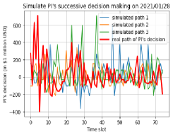
(a)

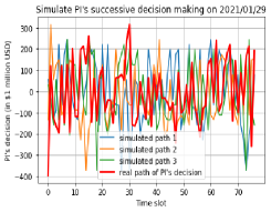
(b)

Figure 5: Simulation of PI’s successive decision making

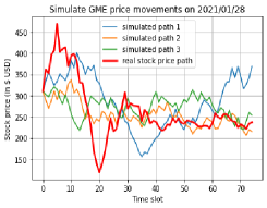
(a)

(b)

Figure 6: Simulation of GME price movements

Step 3: Re-estimate $\Gamma$:

$$z_{i}=\gamma_{t=0}\left(i\right),$$ (25)

$$a_{ij}=\frac{\sum_{t=0}^{T-2}\gamma_{t}\left(i,j\right)}{\sum_{t=0}^{T-2}\gamma_{t}\left(i\right)},$$ (26)

$$b_{i}\left(k\right)=\frac{\sum_{t\in\left\{0,1,\ldots,T-1\right\},s_{t}=\nu{}_{k}}\gamma_{t}\left(i\right)}{\sum_{t=0}^{T-1}\gamma_{t}\left(i\right)},$$ (27)

$$c_{k}\left(l\right)=\frac{\sum_{t\in\left\{0,1,\ldots,T-1\right\},s_{t}=\nu{}_{k},o_{t}=\omega_{l}}\gamma_{t}\left(i\right)}{\sum_{t=0}^{T-1}\gamma_{t}\left(i\right)}.$$ (28)

Step 4: If $P\left(S,O\mid\Gamma\right)=\sum_{i=0}^{J-1}\alpha_{t=\mathrm{T}-1}\left(i\right)$ climbs, go to Step 2, otherwise end the loop.

The parameters of a visible-hidden Markov network are initialized before entering the iterative process and then updated in each iteration until $P\left(S,O\mid\Gamma\right)$ doesn’t grow anymore. $\mathbf{A}$, $\mathbf{B}$, $\mathbf{C}$, and $Z$ are row stochastic, moreover, their rows respectively belong to a standard $J-1$, $J-1$, $K-1$, and $L-1$ simplex which are the support of the Dirichlet distribution of order $J-1$, $J-1$, $K-1$, and $L-1$. Therefore, we can employ the Dirichlet distribution to randomize $\mathbf{A}$, $\mathbf{B}$, $\mathbf{C}$, and $Z$ to keep away from a local maximum which prevents the evolution of the model.

Figure 1c and 1d clearly show that PI’s decision making strategy varies from one episode to another: PI preferred to give a decision with large absolute value at the early stage on Jan. 28, 2021, on the other hand, tended to spread large trades over time on Jan. 29, 2021. In light of these signs, our determination of a visible-hidden Markov network is episode-based. We measure $\Gamma$ in each episode to generate a time series of the probable evolution of PI’s decision making and further transform them to stock price paths through Bayesian inference and regression analysis.

We imitate PI’s successive decision making based on observations from the training dataset $\mathcal{\mathscr{D}}_{i,i=1\ldots 6}$. The hyperparameters are given the following values: $J=2$, and $K=L=30$. We parametrize Dirichlet distribution with $\alpha_{i}=1000$, so that the initial $\mathbf{A}$, $\mathbf{B}$, $\mathbf{C}$, and $Z$ are row stochastic and have near uniform values, where $\alpha_{i}$ denotes any component of the parameter vector $\boldsymbol{\alpha}$. Figure 5 exhibits three simulated paths of PI’s successive decision making along with the real evolution of PI’s decision. In view of article space, we only show the experimental results in two representative episodes for comparison in figures. According to Figure 5a and 5b, we find that the simulated paths on Jan. 29, 2021 are more volatile than those on Jan. 28, 2021. This correctly reflects the discrepancy of the volatility of real PI’s decision on these two days and thus well proves the effectiveness of our algorithm. The B-DNN is trained by the training dataset $\mathcal{\mathscr{D}}_{i,i=1\ldots 6}$ when we perform Bayesian inference in the section III. We continue to carry out regression analysis grounded on this trained B-DNN for each evolutionary path of PI’s decision. For the sake of simplicity, the price change is simulated as its posterior predictive mean. Figure 6 illustrates our simulated price movements of the underlying stock together with the real price path.

V Reinforcement learn option price ground upon imitative PI’s chronological decision making

Our algorithm introduced in the section IV probabilistically imitates PI’s chronological decision making. With the help of B-DNN inference-regression presented in the section III, likely evolutionary paths of PI’s decision are transformed into probable price paths of the underlying stock. These simulated price paths of the underlying stock yield the cross-sectional information for optimizing a dynamically hedged portfolio. This section expounds how to reinforcement learn option price using the cross-sectional information stemmed from imitative PI’s chronological decision making.

Suppose that we sell a European option with the terminal payoff $\mathsf{H}\left(S_{\mathsf{T}}\right)$, where $S_{\mathsf{T}}$ denotes the underlying stock price at expiry date $\mathsf{T}$. For the sake of the suitability of our algorithm for both calls and puts, switching the below expression of the terminal payoff will turn pricing/hedging a call option into a put option:

$$\mathsf{H}\left(S_{\mathsf{T}}\right)=\begin{cases}\max\left(S_{\mathsf{T}}-K,0\right),\mathrm{if\;calls}&\mathrm{}\\ \max\left(K-S_{\mathsf{T}},0\right),\mathrm{if\;puts}.\end{cases}$$ (29)

With the proceeds from the sale of the option, we build a portfolio $\Pi_{t}$ which consists of $a_{t}$ units of the stock with price $S_{t}$ and a deposit in the risk-free bank account $B_{t}$. With the aim of dynamically hedging the option, we rebalance this portfolio to keep its value replicating the value of the option at time $t\leqslant\mathsf{T}$:

$$\Pi_{t}=a{}_{t}S_{t}+B_{t}.$$ (30)

At maturity we close out the position as we no longer need to hedge the option. Consequently, the terminal payoff is the portfolio value at maturity:

$$\Pi_{\mathsf{T}}=\mathsf{H}\left(S_{\mathsf{T}}\right)=B_{t}.$$ (31)

We ignore transaction costs or other frictions in this paper due to the fact that low rates or fixed commissions are offered to the customers with high volume of trades executed (e.g., High-Frequency Trading (HFT) firms). We force our dynamically hedged portfolio $\Pi_{t}$ to be self-financing in such a manner that there is no external infusion or withdrawal of cash over the lifetime of the option, and the spread of portfolio values at different times comes from the continuously compounded risk-free interest rate $r$ and the change in underlying stock price $\bigtriangleup S_{t}$ :

$$\Pi_{t+1}-e^{r}\Pi_{t}=a_{t}\bigtriangleup S_{t}+\kappa f_{\boldsymbol{\theta}^{*}}\left(F\right)a_{t}S_{t},$$ (32)

where $\bigtriangleup S_{t}=S_{t+1}-e^{r}S_{t}$ and $F=\left(a_{t+1}-a_{t}\right)\varTheta S_{t}$.

The cross-sectional information $\mathcal{F}\left(t\right)=\left\{S_{t}^{1},\ldots,S_{t}^{U}\right\}$ collects possible prices at time $t$ from all the simulated price paths, where $U$ is the number of simulated paths and $S_{t}^{u},_{u=1,\ldots,U}$ denotes the price at time $t$ sampled from the $u$th path. Our cross-sectional information is derived from the existing PI’s decision, so we design a compensation term $\kappa f_{\boldsymbol{\theta}^{*}}\left(F\right)a_{t}S_{t}$ to put in the price change caused by our hedging activity if we are also referred to as PI. $f_{\boldsymbol{\theta}^{*}}\left(F\right)$ maps a large-scale volume of buying or selling the underlying stock to a sharp rise or drop in price via our trained B-DNN. We may sell multiple options covering a significant amount of shares of the underlying stock. We use $\varTheta$ to denote the total number of shares of the underlying stock. The coefficient $\kappa$ gives a degree of freedom to scale the compensation term. If we are a single retail investor who sells a mini option, then this compensation term vanishes as $\kappa$ tends to 0. Monte Carlo sample-based reinforcement learning [27] uses the cross-sectional information which is generated by sampling a pre-set probability distribution. Compared with Monte Carlo sample-based reinforcement learning, our algorithm can better fit into each circumstance as we adopt the cross-sectional information that reflects the existing PI’s decision and add an compensation term to compensate for the effect of our hedging activity on the price change.

When price an option at any time within its lifetime, the risk of running out cash to continue rebalancing the portfolio due to the fluctuation in the market price of the underlying stock should be taken into account. To this end, the ask price $\mathcal{C}_{t}$ at time $t\leqslant\mathsf{T}$ is designed to be the sum of the risk free price and the risk-adjustment weighted by the risk-aversion coefficient $\eta$ [27] as expressed in Equation (33). The risk free price is the expected value of the portfolio $\Pi_{t}$. The risk-adjustment accumulates the risk from time $t$ until the expiry date $\mathsf{T}$. The risk at time $t$ is quantized as the expected discounted variance of the portfolio $\Pi_{t}$.

$$\mathcal{C}_{t}\left(S_{t}\right)=\mathbb{E}_{t}\left[\Pi_{t}+\eta\sum_{t^{\prime}=t}^{\mathsf{T}}e^{-r\left(t^{\prime}-t\right)}\mathrm{Var}\left[\Pi_{t^{\prime}}\mid\mathcal{F}_{t^{\prime}}\right]|\mathcal{F}_{t}\right].$$ (33)

Geometric Brownian motion is the most commonly used model of stock price behavior. By applying Itô’s lemma to the random variable of stock price which follows Geometric Brownian motion, the stock price at time $t$ has been proved to be lognormally distributed [28]:

$$\ln S_{t}\sim\mathcal{N}\left(\ln S_{0}+\left(\mu-\frac{\sigma_{s}^{2}}{2}\right)t,\sigma_{s}^{2}t\right),$$ (34)

where $\mu$ is the expected rate of return per time-slot from the stock, and $\sigma_{s}$ is the volatility of the stock price.

Equation (34) implies $S_{t}$ is not martingale due to the constant drift rate $\mu-\frac{\sigma_{s}^{2}}{2}$. When price the option, we prefer the calculation to be based on an independent variable without constant drift. Therefore, we expand the independent variable $S_{t}$ in Equation (30), (32), and (33) to a function in terms of an independent variable without constant drift $\widetilde{S}_{t}$:

$$S_{t}=\exp\left(\widetilde{S}_{t}+\left(\mu-\frac{\sigma_{s}^{2}}{2}\right)t\right).$$ (35)

$S_{t}$ afterwards will signify the expansion of stock price in terms of $\widetilde{S}_{t}$ in all equations.

The following notations will denote for short the other variables which are dependent on $\widetilde{S}_{t}$ in subsequent derivations:

$$\widetilde{a}_{t}=\widetilde{a}_{t}\left(\widetilde{S}_{t}\right)=a_{t},$$ (36)

$$\pi=\pi\left(\widetilde{S}_{t},t\right)=\widetilde{a}_{t},$$ (37)

$$\bigtriangleup S_{t}=e^{\widetilde{S}_{t+1}+\left(\mu-\frac{\sigma_{s}^{2}}{2}\right)\left(t+1\right)}-e^{r}e^{\widetilde{S}_{t}+\left(\mu-\frac{\sigma_{s}^{2}}{2}\right)t},$$ (38)

$$\Pi_{t}=\Pi_{t}\left(\widetilde{S}_{t}\right),$$ (39)

where $\pi$ is the policy function which maps $\widetilde{S}_{t}$ and $t$ to the position in the stock at time $t$.

We are aiming to find a policy to price the option with the satisfaction for the only necessary demand of hedging risk, or other kind of statement, catch the optimal or nearly optimal $\pi$ that minimizes the ask price $\mathcal{C}_{t}\left(\widetilde{S}_{t}\right)$. Our goal can be achieved by using reinforcement learning which translates the aim into learning $\pi$ that maximizes the expected cumulative reward via maximizing the state-value function and the action-value function [29]. Reinforcement learning is found on a MDP. In our scenario, the stock price $\widetilde{S}_{t}\in\mathcal{S}$ is the state and the position in the stock $\widetilde{a}_{t}\in\mathcal{A}$ is the action. Accordingly, the sample space of the stock price $\mathcal{S}$ and the position $\mathcal{A}$ respectively form the state space and the action space. The state-value function for a policy $\pi$ at time $t$ is denoted as $V_{t}^{\pi}\left(\widetilde{S}_{t}\right)$ and it is designed as the negative of the option price. Equation (32) formulates the chronological recursive relationship that expresses the portfolio’s value at time $t$ in respect of its value at the subsequent time $t+1$. We can exploit this chronological recursive relationship to find the Bellman equation for the state-value function and the reward:

$$V_{t}^{\pi}\left(\widetilde{S}_{t}\right)=-\mathcal{C}_{t}\left(\widetilde{S}_{t}\right)$$ (40)

$$=\mathbb{E}_{t}\left[-\Pi_{t}-\eta\sum_{t^{\prime}=t}^{\mathsf{T}}e^{-r\left(t^{\prime}-t\right)}\mathrm{Var}\left[\Pi_{t^{\prime}}\mid\mathcal{F}_{t^{\prime}}\right]|\mathcal{F}_{t}\right]$$ (41)

$$=\mathbb{E}_{t}\left[-\Pi_{t}-\eta\mathrm{Var}\left[\Pi_{t^{\prime}}\right]-\eta\sum_{t^{\prime}=t+1}^{\mathsf{T}}e^{-r\left(t^{\prime}-t\right)}\mathrm{Var}\left[\Pi_{t^{\prime}}\mid\mathcal{F}_{t^{\prime}}\right]|\mathcal{F}_{t}\right]$$ (42)

$$=\mathbb{E}_{t}\left[R_{t}\left(\widetilde{S}_{t},\widetilde{a}_{t},\widetilde{S}_{t+1}\right)+\gamma V_{t+1}^{\pi}\left(\widetilde{S}_{t+1}\right)\right]$$ . (43)

Equation (41) is obtained by plugging Equation (33) into Equation (40). Equation (43) is the Bellman equation for $V_{t}^{\pi}\left(\widetilde{S}_{t}\right)$, where the reward $R_{t}\left(\widetilde{S}_{t},\widetilde{a}_{t},\widetilde{S}_{t+1}\right)$ is derived as below by using the chronological recursive relationship given in Equation (32):

$$R_{t}\left(\widetilde{S}_{t},\widetilde{a}_{t},\widetilde{S}_{t+1}\right) =\gamma\left(\widetilde{a}_{t}\bigtriangleup S_{t}+\kappa f_{\boldsymbol{\theta}^{*}}\left(F\right)S_{t}\right)-\eta\mathrm{Var}\left[\Pi_{t}\mid\mathcal{F}_{t}\right]$$

$$=\gamma\left(\widetilde{a}_{t}\bigtriangleup S_{t}+\kappa f_{\boldsymbol{\theta}^{*}}\left(F\right)S_{t}\right)-\eta\gamma^{2}\mathbb{E}_{t}$$

$$\left[\left(\dot{\Pi}_{t+1}-\left(\widetilde{a}_{t}\bigtriangleup\dot{S}_{t}+\kappa f_{\boldsymbol{\theta}^{*}}\left(F\right)\widetilde{a}_{t}\dot{S}_{t}\right)\right)^{2}\right],$$ (44)

where $\gamma=e^{-r}$ is the discount rate, $\dot{\Pi}_{t+1}=\Pi_{t+1}-\overline{\Pi}{}_{t+1}$, $\bigtriangleup\dot{S}_{t}=\bigtriangleup S_{t}-\bigtriangleup\overline{S}_{t}$, $\dot{S}_{t}=S_{t}-\overline{S}_{t}$, and $\overline{\left(\cdot\right)}$ denotes the sample mean. Maximizing the reward is identical to maximizing the cumulative risk-adjusted return as the last term of the reward stands for the risk at time $t$ and the first term gives the quantized portfolio’s return between time $t$ and $t+1$. When $\eta$ tends to infinity, the hedge becomes a pure risk hedge.

The action-value function ($Q$-function) returns the value of taking action $a$ in state $s$ under a policy $\pi$ at time $t$. Consequently, $Q$-function can be interpreted as a state-value function under the condition of $\widetilde{S}_{t}=s$ and $\widetilde{a}_{t}=a$:

$$Q_{t}^{\pi}\left(s,a\right) =\mathbb{E}_{t}\left[-\Pi_{t}\mid\widetilde{S}_{t}=s,\widetilde{a}_{t}=a\right]$$

$$-\mathbb{E}_{t}\left[\eta\sum_{t^{\prime}=t}^{\mathsf{T}}e^{-r\left(t^{\prime}-t\right)}\mathrm{Var}\left[\Pi_{t^{\prime}}\mid\mathcal{F}_{t^{\prime}}\right]|\widetilde{S}_{t}=s,\widetilde{a}_{t}=a\right].$$ (45)

We use $Q_{t}^{\pi^{\mathit{*}}}\left(\widetilde{S}_{t},\widetilde{a}_{t}^{*}\right)$ to stand for the $Q$-function value which is maximized by the optimal policy $\pi^{\mathit{*}}$ which chooses the optimal action $\widetilde{a}_{t}^{*}$ in state $\widetilde{S}_{t}$ at time $t$:

$$Q_{t}^{\pi^{\mathit{*}}}\left(\widetilde{S}_{t},\widetilde{a}_{t}^{*}\right) =\underset{\pi}{\max}Q_{t}^{\pi}\left(\widetilde{S}_{t},\widetilde{a}_{t}\right)$$

$$=\underset{\widetilde{a}_{t}\in\mathcal{A}}{\max}Q_{t}^{\pi}\left(\widetilde{S}_{t},\widetilde{a}_{t}\right),$$ (46)

where $\pi^{\mathit{*}}=\pi^{*}\left(\widetilde{S}_{t},t\right)$ and $\widetilde{a}_{t}^{*}=\widetilde{a}_{t}^{*}\left(\widetilde{S}_{t}\right)$ are both dependent on $\widetilde{S}_{t}$.

The Bellman optimality equation for the action-value function has a similar structure to the Bellman equation for the state-value function (Equation (43)) and can be expanded by plugging Equation (44) into it:

$$Q_{t}^{\pi}\left(\widetilde{S}_{t},\widetilde{a}_{t}\right)$$

$$= \mathbb{E}_{t}\left[R_{t}\left(\widetilde{S}_{t},\widetilde{a}_{t},\widetilde{S}_{t+1}\right)+\gamma Q_{t+1}^{\pi^{\mathit{*}}}\left(\widetilde{S}_{t+1},\widetilde{a}_{t+1}^{*}\right)\right]$$ (47)

$$= \gamma\mathbb{E}_{t}\left[\widetilde{a}_{t}\bigtriangleup S_{t}+\kappa f_{\boldsymbol{\theta}^{*}}\left(F\right)\widetilde{a}_{t}^{*}S_{t}+Q_{t+1}^{\pi^{\mathit{*}}}\left(\widetilde{S}_{t+1},\widetilde{a}_{t+1}^{*}\right)\right]$$

$$-\eta\gamma^{2}\mathbb{E}_{t}\left[\left(\dot{\Pi}_{t+1}-\left(\widetilde{a}_{t}\bigtriangleup\dot{S}_{t}+\kappa f_{\boldsymbol{\theta}^{*}}\left(F\right)\widetilde{a}_{t}\dot{S}_{t}\right)\right)^{2}\right].$$ (48)

The terminal condition gives the optimal $Q$-function value at expiry in terms of the terminal payoff:

$$Q_{\mathsf{T}}^{\pi^{\mathit{*}}}\left(\widetilde{S}_{\mathsf{T}}^{u},\widetilde{a}_{\mathsf{T}}^{*}\right)=-\mathsf{H}\left(S_{\mathsf{T}}\right)-\mathrm{Var}\left[\mathsf{H}\left(S_{\mathsf{T}}\right)\right],$$ (49)

where $\widetilde{a}_{\mathsf{T}}^{*}=0$.

Our purpose is to find $\pi^{*}\left(\widetilde{S}_{t},t\right)$ or $\widetilde{a}_{t}^{*}\left(\widetilde{S}_{t}\right)$, and $Q_{t}^{\pi^{\mathit{*}}}\left(\widetilde{S}_{t},\widetilde{a}_{t}^{*}\right)$. However, the unknown value of $\widetilde{S}_{t}$ and the incalculable expectation in the Bellman optimality equation prevent us from achieving our goal. For the removal of the barrier, we use the cross-sectional information $\widetilde{\mathcal{F}}=\left\{\widetilde{S}_{t}^{u}\right\}_{u=1,\ldots,U}$ to take as many likely values of $\widetilde{S}_{t}$ into account as possible, where $\widetilde{S}_{t}^{u}=\ln S_{t}^{u}-\left(\mu-\frac{\sigma_{s}^{2}}{2}\right)t$. We believe that our simulated price paths have the same constant drift as those following a lognormal distribution. Moreover, the incalculable expectation in the Bellman optimality equation is approximated by an empirical mean of $U$ observations.

In our scenario, the state space and the action space are both continuous. We adopt basis functions, for example basis-splines, as an intermediary for mapping two continuous spaces. A state sample $\widetilde{S}_{t}$ is first mapped to a set of basis functions and the optimal action $\widetilde{a}_{t}^{*}$ is then expressed as a linear combination of basis functions weighted by the optimal coefficients $w_{nt}^{*}$:

$$\widetilde{a}_{t}^{*}=\sum_{n=1}^{\mathcal{B}}w_{nt}^{*}\psi_{n}\left(\widetilde{S}_{t}\right),$$ (50)

where $\mathcal{B}$ represents the number of basis functions. Similarly, the optimal $Q$-function value can be formulated as a linear combination of basis functions weighted by the optimal coefficients $\varphi_{nt}^{*}$:

$$Q_{t}^{\pi^{\mathit{*}}}\left(\widetilde{S}_{t},\widetilde{a}_{t}^{*}\right)=\sum_{n=1}^{\mathcal{B}}\varphi_{nt}^{*}\psi_{n}\left(\widetilde{S}_{t}\right).$$ (51)

Our objective of finding optimal policy and $Q$-function value is consequently transformed into learning the optimal coefficients $w_{nt}^{*}$ and $\varphi_{nt}^{*}$. We elaborate the derivation of the following closed-form solution of $w_{nt}^{*}$ in Appendix B:

$$w_{t}^{*}=\mathbf{E}_{t}^{-1}\mathbf{D}_{t},$$ (52)

$$E_{nm}^{t} =\sum_{u=1}^{U}\left[\psi_{m}\left(\widetilde{S}_{t}^{u}\right)\bigtriangleup\dot{S}_{t}\varXi\sum_{n=1}^{\mathcal{B}}\psi_{n}\left(\widetilde{S}_{t}^{u}\right)\right]$$

$$+\sum_{u=1}^{U}\left[\kappa f_{\boldsymbol{\theta}^{*}}\left(F\right)\psi_{m}\left(\widetilde{S}_{t}^{u}\right)\dot{S}_{t}\varXi\sum_{n=1}^{\mathcal{B}}\psi_{n}\left(\widetilde{S}_{t}^{u}\right)\right],$$ (53)

$$D_{n}^{t}=\sum_{u=1}^{U}\left[\left(\frac{\bigtriangleup S_{t}^{u}}{2\eta\gamma}+\dot{\Pi}_{t+1}\varXi+\frac{\kappa f_{\boldsymbol{\theta}^{*}}\left(F\right)S_{t}^{u}}{2\eta\gamma}\right)\sum_{n=1}^{\mathcal{B}}\psi_{n}\left(\widetilde{S}_{t}^{u}\right)\right],$$ (54)

$$\varXi=\left(\bigtriangleup\dot{S}_{t}+\kappa f_{\boldsymbol{\theta}^{*}}\left(F\right)\dot{S}_{t}\right),$$ (55)

where $w_{t}^{*}$ is a $\mathcal{B}$-dimensional vector with entry $w_{nt}^{*}$, $\mathbf{E}_{t}$ is a matrix of size $\mathcal{B}\times\mathcal{B}$ with entry $E_{nm}^{t}$ and $\mathbf{D}_{t}$ is a $\mathcal{B}$-dimensional vector with entry $D_{n}^{t}$. We can also introduce a regularization parameter $\varsigma$ with a very small value as $\mathbf{E}_{t}+\varsigma\mathbf{I}_{\mathcal{B}}$. This regularization parameter prevents $\mathbf{E}_{t}$ from becoming a singular matrix which does not have an inverse.

Once we obtain the optimal action $\widetilde{a}_{t}^{*}$ from Equation (52) and Equation (50), the optimal $Q$-function value at time $t$ can be inferred by an expectation in terms of the reward at time $t$ and the optimal $Q$-function value at time $t+1$ through the Bellman optimality equation (Equation (47)) at the optimal action $\widetilde{a}_{t}^{*}$. However, in practice we take the sample from our simulated path instead of the expectation to infer the optimal $Q$-function value at time $t$ and this will produce error $\mathsf{e}_{u}$ which is the deviation of the observed value from the true value:

$$Q_{t}^{\pi^{*}}\left(\widetilde{S}_{t},\widetilde{a}_{t}^{*}\right) =\mathbb{E}_{t}\left[R_{t}\left(\widetilde{S}_{t},\widetilde{a}_{t}^{*},\widetilde{S}_{t+1}\right)+\gamma Q_{t+1}^{\pi^{\mathit{*}}}\left(\widetilde{S}_{t+1},\widetilde{a}_{t+1}^{*}\right)\right]$$

$$=R_{t}\left(\widetilde{S}_{t}^{u},\widetilde{a}_{t}^{*},\widetilde{S}_{t+1}^{u}\right)+\gamma Q_{t+1}^{\pi^{\mathit{*}}}\left(\widetilde{S}_{t+1}^{u},\widetilde{a}_{t+1}^{*}\right)+\mathsf{e}_{u}.$$ (56)

The optimal $Q$-function value at time $t$ can be learned by reaching the criteria of minimizing the sum of squared errors in all simulated paths:

$$\varphi_{nt}^{*} =\min_{\varphi_{nt}}\sum_{u=1}^{U}\mathsf{e}_{u}^{2}$$

$$=\min_{\varphi_{nt}}\sum_{u=1}^{U}\left(F_{u}-\sum_{n=1}^{\mathcal{B}}\varphi_{nt}\psi_{n}\left(\widetilde{S}_{t}^{u}\right)\right)^{2},$$ (57)

where $F_{u}=R_{t}\left(\widetilde{S}_{t}^{u},\widetilde{a}_{t}^{*},\widetilde{S}_{t+1}^{u}\right)+\gamma Q_{t+1}^{\pi^{\mathit{*}}}\left(\widetilde{S}_{t+1}^{u},\widetilde{a}_{t+1}^{*}\right)$.

The optimal coefficients $\varphi_{nt}^{*}$ is approximated by the least square estimator $\widehat{\varphi}_{t}^{*}$:

$$\varphi_{t}^{*} \approx\widehat{\varphi}_{t}^{*}$$

$$=\mathbf{G}_{t}^{-1}\mathbf{H}_{t},$$ (58)

$$G_{nm}^{t}=\psi_{n}\left(\widetilde{S}_{t}^{u}\right)\psi_{m}\left(\widetilde{S}_{t}^{u}\right),$$ (59)

$$H_{n}^{t}=\psi_{n}\left(\widetilde{S}_{t}^{u}\right)\left(R_{t}\left(\widetilde{S}_{t}^{u},\widetilde{a}_{t}^{*},\widetilde{S}_{t+1}^{u}\right)+\gamma Q_{t+1}^{\pi^{\mathit{*}}}\left(\widetilde{S}_{t+1}^{u},\widetilde{a}_{t+1}^{*}\right)\right),$$ (60)

where $\varphi_{t}^{*}$ is a $\mathcal{B}$-dimensional vector with entry $\varphi_{nt}^{*}$, $\mathbf{G}_{t}$ is a matrix of size $\mathcal{B}\times\mathcal{B}$ with entry $G_{nm}^{t}$ and $\mathbf{H}_{t}$ is a $\mathcal{B}$-dimensional vector with entry $H_{n}^{t}$.

We are ultimately able to predict the option price $\mathcal{C}_{t}\left(\widetilde{S}_{t}\right)=-Q_{t}^{\pi^{\mathit{*}}}\left(\widetilde{S}_{t},\widetilde{a}_{t}^{*}\right)$ and the hedge position $\widetilde{a}_{t}^{*}$ backward recursively at any time until the expiration date by triggering the following algorithm:

Algorithm of learning option price and hedge position
1: Calculate $Q_{\mathsf{T}}^{\pi^{\mathit{*}}}\left(\widetilde{S}_{\mathsf{T}}^{u},\widetilde{a}_{\mathsf{T}}^{*}\right)$ with Eq. (49) and $\Pi_{\mathsf{T}}$ with Eq. (31)
2: for $t=\mathsf{T}-1$ to $t=0$ do
3: Calculate $w_{t}^{*}$ with Eq.(52), $\widetilde{a}_{t}^{*}$ with Eq. (50) and $\Pi_{t}$ with Eq. (32)
4: Calculate $R_{t}\left(\widetilde{S}_{t},\widetilde{a}_{t}^{*},\widetilde{S}_{t+1}\right)$ with Eq. (44)
5: Calculate $\varphi_{t}^{*}$ with Eq.(58) and $Q_{t}^{\pi^{\mathit{*}}}\left(\widetilde{S}_{t},\widetilde{a}_{t}^{*}\right)$ with Eq. (51)
6: end for

VI Experimental Evaluation

We evaluate our entire algorithm/process on a task of hedging and pricing an OTC European call option based on 100 shares of the underlying GME stock with a period of 6 trading days and a strike price of 100 USD. Suppose that we have learned that the leading investors are the same group of investors who took on the role as PI during Jan. 26, 2021-Feb. 02, 2021. Therefore, our first step is to probabilistically imitate their previous successive decision making from the hidden motives behind them through our visible-hidden Markov network as we presented in the section IV. The second step is to transform likely evolutionary paths of PI’s decision into probable price paths of the underlying stock by our B-DNN inference-regression process introduced in the section III.

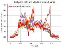
(a)

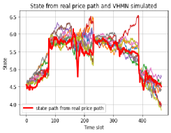
(b)

Figure 7: Imitative GME price movements

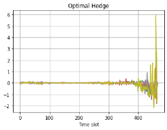
(a)

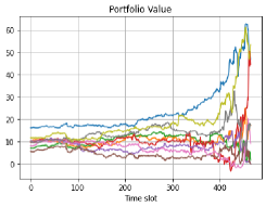
(b)

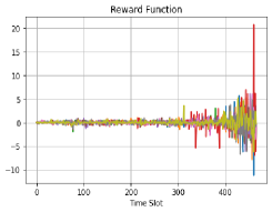
(c)

(d)

Figure 8: Reinforcement learn option price and hedging position ground upon imitative PI’s chronological decision making

For the above two steps, we train a B-DNN and a visible-hidden Markov network on an episode basis with the training data set $\mathcal{\mathscr{D}}_{i,i=1\ldots 6}$. The simulated price paths along with the real price paths used as the training data samples are compared in Figure 7a. We remove the constant drift from all the price paths and plot the real state $\widetilde{S}_{t}$ and the simulated states $\widetilde{S}_{t}^{u}$ in Figure 7b. The drift rate is calculated with $\mu=0.05$ and $\sigma_{s}=0.2926$. The value of $\sigma_{s}$ is derived from averaging the daily VIX index from Jan. 26, 2021 to Feb. 02, 2021. The total number of the simulated paths is 1000 and only 10 paths are uniformly sampled to be shown here. The training samples are sampled in each 5-minute time slot. The simulated paths are also with a time resolution of 5 minutes. The price jumps that appear in Figure 7a and 7b are from the pricing data in the first 5-min time slot (i.e., 09:30 to 09:35). The open price and the volume in this time slot deviate far from the average owing to their high dependence on the pre-market trading and news. For this reason, the training dataset does not include the pricing data in the first 5-min time slot, and we interpolate the real value in the figures. The Visible-hidden Markov network is abbreviated to VHMN in the figures for the benefit of space. We can observe that the visible-hidden Markov network produces imitative price paths that have a highly matched behavior pattern with the real price path. As a consequence, the visible-hidden Markov network is a powerful tool to cope with the intrinsic instability in financial data by engendering imitative variations for each specific scenario.

Our final phase of this task is to perform the algorithm of learning option price and hedge position. We rebalance the portfolio every 5 minutes during 6 trading days. The risk-free interest rate $r=1.059\%$ is taken as the average of daily US 10-year bond yield from Jan. 26, 2021 to Feb. 02, 2021. We set $\kappa=0$ as we only hedge a mini option based on 100 shares. We also give $\frac{1}{\eta}=0$ for having pure risk hedge. $\varsigma=0.001$ is used to avoid the error of inverting a singular matrix. The optimal hedging position is shown in Figure (8a), where the value on the graph needs to be multiplied by 100 to correspond to 100 shares. It is exhibited that the option is more actively hedged when closer to the expiration date. The value of the replicating portfolio jumps near the maturity date and the hedging strategy effectively protects the portfolio against the risk of running out of money as shown in Figure (8b). The optimal $Q$-function value converges at -27.586 which means we better sell the option at the price of 2758.6 USD as illustrated in Figure (8d).

VII Conclusion

In order to address the challenges posed by intrinsic low SNR and instability in financial data, we innovatively exploit imitative cross-sectional information to learn option price and hedging position with reinforcement learning. When we turn to behavior finance, another challenge of identifying the leading investor’s behavior and the stock price change comes along. To this end, we take advantage of the excellent features of B-DNN to explore non-deterministic relations in a market data driven fashion.

Appendix A

Denote likelihood times prior as $a\left(\boldsymbol{\theta}\right)\coloneqq p\left(\mathcal{\mathscr{D}}\mathrm{|\boldsymbol{\theta}}\right)p\left(\boldsymbol{\theta}\right)$ which satisfies 2nd-order sufficient conditions: $a^{\prime}\left(\boldsymbol{\theta}^{\ast}\right)=\boldsymbol{0}$ and $a^{\prime\prime}\left(\boldsymbol{\theta}^{\ast}\right)$ is positive definite, where $\boldsymbol{\theta}^{\ast}$ is a strict local maximizer. We do a Taylor series approximation of $\log a\left(\boldsymbol{\theta}\right)$ around the location of its maximum to give:

$$\log a\left(\boldsymbol{\theta}\right)\approx\log a\left(\boldsymbol{\theta}^{\ast}\right)+\frac{1}{2}\left(\boldsymbol{\theta}-\boldsymbol{\theta}^{\ast}\right)^{T}\nabla_{\boldsymbol{\theta\theta}}^{2}\log a\left(\boldsymbol{\theta}^{\ast}\right)\left(\boldsymbol{\theta}-\boldsymbol{\theta}^{\ast}\right)$$ (61)

Plugging this truncated Taylor expansion of $\log a\left(\boldsymbol{\theta}\right)$ into the posterior $P\left(\mathrm{\boldsymbol{\theta}}|\mathcal{\mathscr{D}}\right)$ will demonstrate the posterior as the gaussian distribution $\mathcal{N}\left(\boldsymbol{\theta}\mid\boldsymbol{\theta}^{\ast},\left[-\nabla_{\boldsymbol{\theta\theta}}^{2}\log a\left(\boldsymbol{\theta}^{\ast}\right)\right]^{-1}\right)$:

$$P\left(\mathrm{\boldsymbol{\theta}}|\mathcal{\mathscr{D}}\right) =\frac{P\left(\mathcal{\mathscr{D}}\mathrm{|\boldsymbol{\theta}}\right)P\left(\boldsymbol{\theta}\right)}{\int P\left(\mathcal{\mathscr{D}}\mathrm{|\boldsymbol{\theta}}\right)P\left(\boldsymbol{\theta}\right)d\boldsymbol{\theta}}$$

$$=\frac{\exp\left(\log a\left(\boldsymbol{\theta}\right)\right)}{\int\exp\left(\log a\left(\boldsymbol{\theta}\right)\right)d\boldsymbol{\theta}}$$

$$\approx\frac{\exp\left(-\frac{1}{2}\left(\boldsymbol{\theta}-\boldsymbol{\theta}^{\ast}\right)^{T}\left[-\nabla_{\boldsymbol{\theta\theta}}^{2}\log a\left(\boldsymbol{\theta}^{\ast}\right)\right]\left(\boldsymbol{\theta}-\boldsymbol{\theta}^{\ast}\right)\right)}{\int\exp\left(-\frac{1}{2}\left(\boldsymbol{\theta}-\boldsymbol{\theta}^{\ast}\right)^{T}\left[-\nabla_{\boldsymbol{\theta\theta}}^{2}\log a\left(\boldsymbol{\theta}^{\ast}\right)\right]\left(\boldsymbol{\theta}-\boldsymbol{\theta}^{\ast}\right)\right)d\boldsymbol{\theta}}$$

$$=\frac{\exp\left(-\frac{1}{2}\left(\boldsymbol{\theta}-\boldsymbol{\theta}^{\ast}\right)^{T}\left[-\nabla_{\boldsymbol{\theta\theta}}^{2}\log a\left(\boldsymbol{\theta}^{\ast}\right)\right]\left(\boldsymbol{\theta}-\boldsymbol{\theta}^{\ast}\right)\right)}{\sqrt{2\pi\left[-\nabla_{\boldsymbol{\theta\theta}}^{2}\log a\left(\boldsymbol{\theta}^{\ast}\right)\right]^{-1}}}$$ (62)

When we enforce the likelihood and the prior belong to the exponential family with the following expression $P\left(\mathscr{D}\mid\boldsymbol{\theta}\right)\coloneqq\frac{e^{-L\left(\boldsymbol{\theta},\mathscr{D}\right)}}{\int e^{-L\left(\boldsymbol{\theta},\mathscr{D}\right)}d\boldsymbol{\theta}}$ and $P\left(\boldsymbol{\theta}\right)\coloneqq\frac{e^{\mathit{-r}\left(\boldsymbol{\boldsymbol{\theta}}\right)}}{\int e^{\mathit{-r}\left(\boldsymbol{\boldsymbol{\theta}}\right)}d\boldsymbol{\theta}}$, the gaussian distribution followed by the posterior becomes $\mathcal{N}\left(\boldsymbol{\theta}\mid\boldsymbol{\theta}^{\ast},\left[\nabla_{\boldsymbol{\theta\theta}}^{2}L\left(\boldsymbol{\theta}^{\ast},\mathscr{D}\right)+\lambda\mathbf{I}_{\mathit{M}}\right]^{-1}\right)$, where $\mathbf{I}_{\mathit{M}}$ is an identity matrix of size $M\times M$.

Appendix B

From Equation (48) and Equation (50), we know $Q_{t}^{\pi}\left(\widetilde{S}_{t},\widetilde{a}_{t}\right)$ is a quadratic function of $\widetilde{a}_{t}$ and $\widetilde{a}_{t}$ is a linear function of $w_{nt}$. Therefore, finding the optimal coefficients $w_{nt}^{*}$ which maximize $Q$-function value is equivalent to solving the following equation $\frac{-\partial Q_{t}^{\pi}\left(\widetilde{S}_{t},\widetilde{a}_{t}\right)}{\partial w_{nt}}\mid_{w_{nt}=w_{nt}^{*}}=0$:

$$\frac{-\partial Q_{t}^{\pi}\left(\widetilde{S}_{t},\widetilde{a}_{t}\right)}{\partial w_{nt}}$$

$$=\frac{-\partial Q_{t}^{\pi}\left(\widetilde{S}_{t},\widetilde{a}_{t}\right)}{\partial\widetilde{a}_{t}}\frac{\partial\widetilde{a}_{t}}{\partial w_{nt}}$$

$$=\mathbb{E}_{t}\left[\left(\bigtriangleup S_{t}+\kappa f_{\boldsymbol{\theta}^{*}}\left(F\right)S_{t}\right)\sum_{n=1}^{N}\psi_{n}\left(\widetilde{S}_{t}\right)\right]-2\eta\gamma\mathbb{E}_{t}\left[\left(\dot{\Pi}_{t+1}-\left(\widetilde{a}_{t}\bigtriangleup\dot{S}_{t}+\kappa f_{\boldsymbol{\theta}^{*}}\left(F\right)\widetilde{a}_{t}\dot{S}_{t}\right)\right)\left(-\bigtriangleup\dot{S}_{t}-\kappa f_{\boldsymbol{\theta}^{*}}\left(F\right)\dot{S}_{t}\right)\sum_{n=1}^{\mathcal{B}}\psi_{nt}\left(\widetilde{S}_{t}\right)\right]$$

$$\approx\frac{1}{U}\sum_{u=1}^{U}\left[\left(\bigtriangleup S_{t}^{u}+\kappa f_{\boldsymbol{\theta}^{*}}\left(F\right)S_{t}^{u}\right)\sum_{n=1}^{\mathcal{B}}\psi_{nt}\left(\widetilde{S}_{t}^{u}\right)\right]$$

$$\frac{-2\eta\gamma}{U}\sum_{u=1}^{U}\left[\left(\dot{\Pi}_{t+1}-\left(\widetilde{a}_{t}\bigtriangleup\dot{S}_{t}^{u}+\kappa f_{\boldsymbol{\theta}^{*}}\left(F\right)\widetilde{a}_{t}\dot{S}_{t}^{u}\right)\right)\left(-\bigtriangleup\dot{S}_{t}^{u}-\kappa f_{\boldsymbol{\theta}^{*}}\left(F\right)\dot{S}_{t}^{u}\right)\sum_{n=1}^{\mathcal{B}}\psi_{nt}\left(\widetilde{S}_{t}^{u}\right)\right]$$ , (63)

$$\frac{-\partial Q_{t}^{\pi}\left(\widetilde{S}_{t},\widetilde{a}_{t}\right)}{\partial w_{nt}}\mid_{w_{nt}=w_{nt}^{*}}=0 \Rightarrow$$

$$\sum_{u=1}^{U}\left[\left(\frac{\bigtriangleup S_{t}^{u}}{2\eta\gamma}+\dot{\Pi}_{t+1}\varXi+\frac{\kappa f_{\boldsymbol{\theta}^{*}}\left(F\right)S_{t}^{u}}{2\eta\gamma}\right)\sum_{n=1}^{\mathcal{B}}\psi_{n}\left(\widetilde{S}_{t}^{u}\right)\right]=$$

$$\sum_{u=1}^{U}\left[\left(\sum_{m=1}^{\mathcal{B}}w_{mt}^{*}\psi_{m}\left(\widetilde{S}_{t}^{u}\right)\bigtriangleup\dot{S}_{t}\varXi+\kappa f_{\boldsymbol{\theta}^{*}}\left(F\right)\sum_{m=1}^{\mathcal{B}}w_{mt}^{*}\psi_{m}\left(\widetilde{S}_{t}^{u}\right)\dot{S}_{t}\varXi\right)\sum_{n=1}^{\mathcal{B}}\psi_{n}\left(\widetilde{S}_{t}^{u}\right)\right] \Rightarrow$$

$$D_{n}^{t}=\sum_{m=1}^{\mathcal{B}}E_{nm}^{t}w_{mt}^{*},n=1\ldots\mathcal{B} \Rightarrow$$

$$w_{t}^{*}=\mathbf{E}_{t}^{-1}\mathbf{D}_{t}$$ , (64)

where $w_{t}^{*}$ is a $\mathcal{B}$-dimensional vector with entry $w_{nt}^{*}$. $\mathbf{E}_{t}$ and $\mathbf{D}_{t}$ are respectively a matrix of size $\mathcal{B}\times\mathcal{B}$ and a $\mathcal{B}$-dimensional vector. Their entries $E_{nm}^{t}$ and $D_{n}^{t}$ are formulated below:

$$E_{nm}^{t}=\sum_{u=1}^{U}\left[\left(\psi_{m}\left(\widetilde{S}_{t}^{u}\right)\bigtriangleup\dot{S}_{t}\varXi+\kappa f_{\boldsymbol{\theta}^{*}}\left(F\right)\psi_{m}\left(\widetilde{S}_{t}^{u}\right)\dot{S}_{t}\varXi\right)\sum_{n=1}^{\mathcal{B}}\psi_{n}\left(\widetilde{S}_{t}^{u}\right)\right],$$

$$D_{n}^{t}=\sum_{u=1}^{U}\left[\left(\frac{\bigtriangleup S_{t}^{u}}{2\eta\gamma}+\dot{\Pi}_{t+1}\varXi+\frac{\kappa f_{\boldsymbol{\theta}^{*}}\left(F\right)S_{t}^{u}}{2\eta\gamma}\right)\sum_{n=1}^{\mathcal{B}}\psi_{n}\left(\widetilde{S}_{t}^{u}\right)\right],$$

$$\varXi=\left(\bigtriangleup\dot{S}_{t}+\kappa f_{\boldsymbol{\theta}^{*}}\left(F\right)\dot{S}_{t}\right).$$

References

- [1] Black, F., Scholes, M., 1973. The pricing of options and corporate liabilities. Journal of Political Economy 81, 637–654.
- [2] Merton, R.C., 1976. Option pricing when underlying stock returns are discontinuous. Journal of Financial Economics 3, 125–144.
- [3] Heston, S., 1993. Closed-form solution for options with stochastic volatility, with application to bond and currency options. Review of Financial Studies 6, 327–343.
- [4] Bauwens, L., Laurent, S., Rombouts, J.V.K. (2005). “Multivariate GARCH models: A survey”. Journal of Applied Econometrics. In press.
- [5] G. E. Monahan, “State of the art—a survey of partially observable markov decision processes: theory, models, and algorithms,” Management science, vol. 28, no. 1, pp. 1–16, 1982.
- [6] Jospin, L. V., Buntine, W., Boussaid, F., Laga, H., and Bennamoun, M., “Hands-on bayesian neural networks–a tutorial for deep learning users,” arXiv preprint arXiv:2007.06823, 2020.
- [7] Radford M. N., “Bayesian Learning for Neural Networks,” Springer-Verlag, Berlin, Heidelberg, 1996. ISBN 0387947248.
- [8] S. Sun, G. Zhang, J. Shi, and R. Grosse, “Functional Variational Bayesian Neural Networks,” arXiv preprint arXiv:1903.05779, 2019.
- [9] Wang, H.; Yeung, D.Y. A survey on Bayesian deep learning. ACM Comput. Surv. (CSUR) 2020, 53, 1–37.
- [10] Keynes, J. M. (1936). The General Theory of Employment, Interest and Money. New York: Harcourt Brace and Co.
- [11] Gao, P. (2008). Keynesian beauty contest, accounting disclosure, and market efficiency. Journal of Accounting Research, 46:785–807.
- [12] A. A. Adebiyi, A. O. Adewumi, C. K. Ayo, “Stock Price Prediction Using the ARIMA Model,” in UKSim-AMSS 16th International Conference on Computer Modeling and Simulation., 2014.
- [13] M. Khashei, M. Bijari, S. R. Hejazi, Combining seasonal arima models with computational intelligence techniques for time series forecasting, Soft Computing 16 (6) (2012) 1091–1105.
- [14] P. Mantalos, A. Karagrigoriou, L. Strelec, P. Jordanova, P. Hermann, J. Kiselak, J. Hudak, and M. Stehlik, Journal of Applied Statistics, “On improved volatility modelling by fitting skewness in ARCH models,” Volume 47, 2020 - Issue 6.
- [15] Fischer, T. and Krauss, C. (2017). Deep learning with long short-term memory networks for financial market predictions. European Journal of Operational Research.
- [16] Z. Berradi and M. Lazaar, “Integration of principal component analysis and recurrent neural network to forecast the stock price of casablanca stock exchange,” Procedia computer science, vol. 148, pp. 55–61, 2019.
- [17] Raehyun Kim, Chan Ho So, Minbyul Jeong, Sanghoon Lee, Jinkyu Kim, and Jaewoo Kang. Hats: A hierarchical graph attention network for stock movement prediction. arXiv preprint arXiv:1908.07999, 2019.
- [18] Daiki Matsunaga, Toyotaro Suzumura, and Toshihiro Takahashi. 2019. Exploring graph neural networks for stock market predictions with rolling window analysis. ArXiv, abs/1909.10660.
- [19] M. Ugur Gudelek, S. Arda Boluk, and A. Murat Ozbayoglu. A deep learning based stock trading model with 2-d cnn trend detection. In 2017 IEEE Symposium Series on Computational Intelligence (SSCI). IEEE, November 2017.
- [20] Hoseinzade, E.; Haratizadeh, S. CNNpred: CNN-based stock market prediction using a diverse set of variables. Expert Syst. Appl. 2019, 129, 273–285.
- [21] Mohammad E. K., Alexander I., Ehsan A., and Maciej K., “Approximate inference turns deep networks into Gaussian processes,” Advances in neural information processing systems, 2019.
- [22] Rasmussen C. E. and Williams C. K. I., “Gaussian Processes for Machine Learning,” Cambridge, MA, USA: MIT Press, 2006.
- [23] Rue, H., Martino, S. and Chopin, N. (2009). Approximate Bayesian inference for latent Gaussian models by using integrated nested Laplace approximations. Journal of the Royal Statistical Society: Series B (Statistical Methodology) 71 319–392.
- [24] K. Kristensen, A. Nielsen, C. W. Berg, H. Skaug, and B. Bell. TMB: Automatic Differentiation and Laplace Approximation. Journal of Statistical Software, 70(1):1–21, 2016.
- [25] L. Tierney and J. B. Kadane, “Accurate approximations for posterior moments and marginal densities,” J. Amer. Statistical Assoc., vol. 81, no. 393, pp. 82–86, 1986.
- [26] Stamp, M.: A revealing introduction to hidden Markov models. http://www.cs.sjsu.edu/~stamp/RUA/HMM.pdf (2011)
- [27] I. Halperin. QLBS: Q-learner in the Black-Scholes (-Merton) worlds. arXiv:1712.04609, 2017.
- [28] J. Hull, Options, Futures, and Other Derivatives, 6th ed., Englewood Cliffs, NJ, USA: Prentice-Hall, 2006.
- [29] Richard Sutton and Andrew Barto. Reinforcement Learning: An Introduction. MIT Press, 1998.