Large-Scale Attribute-Object Compositions

Abstract.

We study the problem of learning how to predict attribute-object compositions from images, and its generalization to unseen compositions missing from the training data. To the best of our knowledge, this is a first large-scale study of this problem, involving hundreds of thousands of compositions. We train our framework with images from Instagram using hashtags as noisy weak supervision. We make careful design choices for data collection and modeling, in order to handle noisy annotations and unseen compositions. Finally, extensive evaluations show that learning to compose classifiers outperforms late fusion of individual attribute and object predictions, especially in the case of unseen attribute-object pairs.

broken

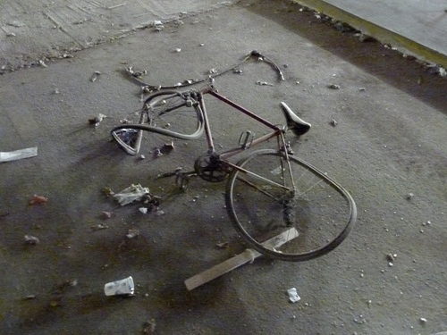
electric

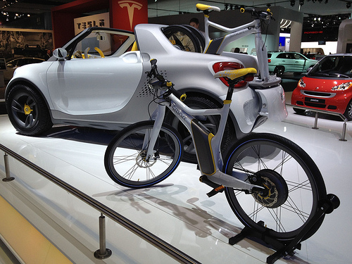
bicycle              clock              flower

Figure 1. Example attribute-object compositions predicted by our approach in the YFCC100m dataset (Thomee et al., 2015).

1. Introduction

Attributes are interpretable visual qualities of objects, such as colors, materials, patterns, shapes, sizes, etc. Their recognition from images has been explored in computer vision, both as specific attributes for faces (Kumar et al., 2008; Liu et al., 2015; Wang et al., 2016), people (Deng et al., 2014; Wang et al., 2019), and e-commerce products (Berg et al., 2010; Hsiao and Grauman, 2017), as well as generic attributes for objects (Lampert et al., 2009; Farhadi et al., 2009) and scenes (Patterson and Hays, 2012; Laffont et al., 2014). Attributes have been used to facilitate visual content understanding in applications such as image retrieval (Kumar et al., 2011), product search (Kovashka et al., 2012), zero-shot object recognition (Al-Halah et al., 2016), image generation (Yan et al., 2016; Georgopoulos et al., 2020), etc.

Compared to object classification, where annotating a single dominant object per image is typically enough to train a robust system, attribute prediction requires more complex annotations. An object can often be described by ten or more prominent attributes of different types. For example, a skirt could be red, blue, striped, long, and ruffled. Other objects may share these same attributes, e.g. a pair of pants might be striped, corduroy and blue, suggesting the task of generalizing to new combinations (blue pants) from past learnings (blue skirts). Attribute prediction has been under-explored compared to object classification, and the complexity of obtaining good attribute annotations is likely a factor. Most of the existing labeled attribute datasets lack scale, cover only a narrow set of objects, and are often only partially annotated.

In this work we focus on the problem of joint attribute-object classification, i.e., learning to simultaneously predict not only the objects in an image but also the attributes associated with them, see Figure 1. This poses significant scientific and engineering challenges, mostly due to the large (quadratic) nature of the label space. As an example, 1000 objects and 1000 attributes would already lead to 1M attribute-object combinations. Generating annotations for every combination is therefore impractical, if not infeasible. In addition, some combinations are very rare, and we may not be able to find any training sample for them, even if they may still appear in the wild: they are unseen at training time but can still arise at inference time in a real-world system. Most previous works model attributes independently of objects, wishfully hoping that the acquired knowledge about an attribute will transfer to a novel category. This reduces the number of training images and annotations required but sacrifices robustness. On the other hand, work on joint visual modeling of attributes and objects, with analysis on the generalization to unseen combinations, is practically nonexistent.

To address these challenges we propose an end-to-end, weakly-supervised composition framework for attribute-object classification. To obtain training data and annotations we build upon the weakly-supervised work of Mahajan et al. (Mahajan et al., 2018), that uses Instagram hashtags as object labels to train the models. However, curating a set of hashtag adjectives is a challenging problem by itself, as, unlike nouns, they are mostly non-visual. We propose an additional hashtag engineering step, in which attributes are selected in a semi-automatic manner to fit the desired properties of visualness, sharedness across objects, and interpretability. Our final training dataset consists of $78M$ images spanning $7694$ objects, $1237$ attributes, and $280k$ compositions with at least $100$ occurrences, which is significantly larger than any attribute-based dataset in number of images and categories.

We also propose a multi-head architecture with three output classifier heads: (i) object classifiers; (ii) object-agnostic attribute classifiers; and, (iii) attribute-object classifiers. Instead of explicitly learning a linear classifier for every attribute-object fine-grain combination – which has high requirements in terms of memory and computation, and has limited generalization– and motivated by the work of Misra et al. (Misra et al., 2017), we incorporate a module that composes these classifiers by directly reasoning about them in the classifier space. This composition module takes the object and attribute classifier weights from the network and learns how to compose them into attribute-object classifiers. Crucially, this allows the model to predict, at inference time, combinations not seen during training.

We show that a vanilla implementation of the composition network has performance and scalability issues when trained on our noisy dataset with missing object and attribute labels. Hence, we propose a set of crucial design changes to make the composition network effective in our real-world setting. These choices include a more suitable loss function that caters better to dataset noise and a selection strategy to reduce the set of candidate attribute-object combinations considered during training and inference.

Finally, we extensively evaluate our method at different data scales by testing the performance on both seen and unseen compositions and show the benefits of explicitly learning compositionality instead of using a late fusion of individual object and attribute predictions. Additionally, to advocate the usage of the proposed framework beyond weakly-supervised learning, we evaluate its effects on our internal Marketplace dataset with cleaner labels.

2. Related Work

Object classification and weak supervision.

Object classification and convolutional neural networks attracted a lot of attention after the success of Krizhevsky et al. (Krizhevsky et al., 2012). Their success is mainly due to the use of very large annotated datasets, e.g. ImageNet (Russakovsky et al., 2015), where the acquisition of the training data requires a costly process of manual annotation. Training convolutional networks on a very large set of weakly-supervised images by defining the proxy tasks using the associated meta-data has shown additional benefits for the image-classification task (Denton et al., 2015; Joulin et al., 2016; Gross et al., 2017; Sun et al., 2017; Li et al., 2017; Mahajan et al., 2018; Veit et al., 2018). Some examples of proxy tasks are hashtag prediction (Denton et al., 2015; Gross et al., 2017; Mahajan et al., 2018; Veit et al., 2018), search query prediction (Sun et al., 2017), and word n-gram prediction (Joulin et al., 2016; Li et al., 2017).

Our approach builds upon the work of Mahajan et al. (Mahajan et al., 2018) which learns to predict hashtags on social media images, after a filtering procedure that matches hashtags to noun synsets in WordNet (Miller, 1995). We extend these noun synsets with adjective synsets corresponding to visual attributes. Unlike object-related nouns, that are mostly visual, most of the attributes selected in this a manner were non-visual, and required us to apply an additional cleaning procedure.

Visual attribute classification.

We follow the definition of visual attributes by Duan et al. (Duan et al., 2012): Attributes are visual concepts that can be detected by machines, understood by humans, and shared across categories. The mainstream approach to learn attributes is very similar to the approach used to learn object classes: training a convolutional neural network with discriminative classifiers and carefully annotated image datasets (Liu et al., 2015; Wang et al., 2016; Singh and Lee, 2016; Su et al., 2016; Lu et al., 2017). Furthermore, labeled attribute image datasets either lack the data scale (Kumar et al., 2009; Lampert et al., 2009; Russakovsky and Fei-Fei, 2010; Patterson and Hays, 2012; Chen et al., 2012; Isola et al., 2015; Patterson and Hays, 2016; Zhao et al., 2019) common to the object datasets, contain a small number of generic attributes (Lampert et al., 2009; Russakovsky and Fei-Fei, 2010), and/or cover few specific categories such as person (Liu et al., 2011; Sharma and Jurie, 2011), faces (Kumar et al., 2009; Liu et al., 2015), clothes (Chen et al., 2012; Yu and Grauman, 2014; Liu et al., 2016), animals (Lampert et al., 2009), scenes (Patterson and Hays, 2012). In this work, we explore learning diverse attributes and objects from large-scale weakly-supervised datasets.

Composition classification.

The basic idea of compositionality is that new concepts can be constructed by combining the primitive ones. This idea was previously explored in natural language processing (Mitchell and Lapata, 2008; Baroni and Zamparelli, 2010; Guevara, 2010; Socher et al., 2013; Nguyen et al., 2014), and more recently in vision (Sadeghi and Farhadi, 2011; Pezzelle et al., 2016; Zhang et al., 2017; Chen and Grauman, 2014; Misra et al., 2017; Nagarajan and Grauman, 2018; Santa Cruz et al., 2018). Compositionality in vision can be grouped into following modeling paradigms: object-object (noun-noun) combinations (Pezzelle et al., 2016), object-action-object (noun-verb-noun) interactions (Sadeghi and Farhadi, 2011; Zhang et al., 2017), attribute-object (adjective-noun) combinations (Chen and Grauman, 2014; Misra et al., 2017; Nagarajan and Grauman, 2018), and complex logical expressions of attributes and objects (Santa Cruz et al., 2018; Chen et al., 2020). In this work, we focus on the attribute-object compositionality.

Prior work also focuses on the unseen compositions paradigm (Chen and Grauman, 2014; Misra et al., 2017; Nagarajan and Grauman, 2018), where a part of the composition space is seen at the training time, while new unseen compositions appear at inference, as well. Towards that end, Chen and Grauman (Chen and Grauman, 2014) employ tensor completion to recover the latent factors for the 3D attribute-object tensor, and use them to represent the unobserved classifier parameters. Misra et al. (Misra et al., 2017) combine pre-trained linear classifier weights (vectors) into a new compositional classifier, using a multilinear perceptron (MLP) which is trained with seen compositions but shows generalization abilities to unseen ones. Finally, Nagarajan and Grauman (Nagarajan and Grauman, 2018) model attribute-object composition as an attribute-specific invertible transformation (matrix) on object vectors.

Motivated by the idea from Misra et al. (Misra et al., 2017), we combine attribute and object classifier weights with an MLP to produce composition classifiers. Unlike (Misra et al., 2017), we learn these constituent classifiers in a joint end-to-end pipeline together with image features and compositional MLP network. As discussed during the introduction, further design changes (e.g. changes in the loss and the composition selection) are also required in a large-scale, weakly-supervised setting.

3. Modeling

In this section we first describe the data collection process to create our datasets. Then, we discuss the full pipeline architecture and loss functions employed to jointly train it in an end-to-end fashion. Finally, we describe our efficient inference procedure, which does not require computing predictions for all the compositions.

3.1. Training and Evaluation Data

3.1.1. Instagram Datasets

We follow the data collection pipeline of (Mahajan et al., 2018), extended for the purpose of collecting attribute hashtags in addition to object hashtags. This simple procedure collects public images from Instagram after matching their corresponding hashtags to WordNet synsets (Miller, 1995): (i) We select a set of hashtags corresponding to noun synsets for the objects, and adjective synsets for the attributes. (ii) To better fit the compositional classification task, we download images that are tagged with at least one hashtag from the object set and at least one hashtag from the attribute set. (iii) Next, we apply a hashtag deduplication procedure (Mahajan et al., 2018), that utilizes WordNet synsets (Miller, 1995) to merge multiple hashtags with the same meaning into a single canonical form (e.g., #brownbear and #ursusarctos are merged). In addition, for adjectives only, we merge relative attributes into a single canonical form, as well, (e.g., #small, #smaller, #smallest). (iv) Finally, for each downloaded image, each hashtag is replaced with its canonical form. The canonical hashtags for objects, attributes, and their pairwise compositions are used as label sets for training and inference.

Attribute visualness, sharedness, and interpretability.

Unlike object (noun) classes, that are mostly visual, attribute (adjective) classes are often non-visual and tend to be noisier. In addition to the hashtag filtering applied in (Mahajan et al., 2018), we apply two automatic strategies to clean them. These strategies are inspired by the attribute definition, i.e., we would like them to be recognizable by computer vision (visualness), and they should be shared across objects (sharednesss).

We implement a similar strategy as in (Berg et al., 2010) to generate a visualness score for each attribute: (i) We start by training linear classifiers for all attributes on top of image features from (Mahajan et al., 2018). (ii) We then evaluate precision@5 for each attribute on a held out validation set, and use it as a visualness score. Examples of attributes that have low visualness score: #inspired, #talented, #firsthand, #atheist.

To evaluate attribute sharedness across objects, we analyse their co-occurrence statistics. For a given attribute, sharedness score is defined as the number of objects it occurs more than 100 times with, weighted by the logarithm of inverse attribute frequency. These scores are finally normalized to $[0,1]$ range, to be comparable with visualness score. For example, #aerodynamic attribute has a high visualness score, but occurs exclusively with #airplane category, thus having a low sharedness score.

Finally, we rank attributes based on the product of their visualness and sharedness score, and manually select those that are interpretable by humans based on a small set of random images associated with their respective hashtags. This is done to make sure visual attributes are representing object features that a user would use to express themselves in, for example, product search. The filtering procedure is lightweight, as the head of the ranked list already provides a very clean set of attributes. For reference, the full list of adjective hashtags contains 10k entries, and only 1237 are selected to satisfy all three properties. By combining attributes with the objects they describe, we create the following two datasets of different scale, to be used in the experimental analysis.

IG-504-144.

A dataset with 504 object and 144 attribute categories. It contains 8904 attribute-object compositions with at least 100 occurrences. In order to evaluate the unseen scenario, we randomly split the compositions with a 20/80% ratio, i.e., 1729 (20%) compositions are selected as unseen and 7175 (80%) as seen. We then label all images that contain at least one of unseen compositions as unseen, and the rest as seen. The train partition contains 2.5M images selected from the seen image split only. The test partition contains 740k images selected from both seen and unseen splits.

IG-8k-1k.

A dataset with 7694 object and 1237 attribute categories. It contains more than 280k attribute-object compositions with at least 100 occurrences. In this case, we split the compositions with a 30/70% ratio, i.e., 83461 (30%) compositions are selected as unseen and 196646 (70%) as seen. The train partition contains 78M images images selected from the seen image split only. The test partition contains 890k images selected from both seen and unseen splits.

This dataset is significantly larger than any other publicly available dataset containing attributes, both in the number of images and class set size, while covering a wide variety of object categories. Note that our train and test datasets are weakly-supervised, and thus suffer from a considerable amount of noise.

3.1.2. Marketplace Dataset

To verify that our weakly-supervised evaluation translates to the fully-supervised scenario, we also evaluate our method on the internal Marketplace dataset. This dataset is smaller in scale than our largest Instagram dataset, but the test data is collected in a fully-supervised setting with human supervision.

We leverage the Marketplace C2C (customer-to-customer) image dataset, which contains public images uploaded by users on the platform for selling their product items to other users. We follow a two-level taxonomy where the first level describes the attribute types (color, pattern, embellishments, etc) and the leaf level describes the attribute values (red, blue, polka dot, fringe, etc). This dataset contains 6M train and 238k test images spanning across 992 product categories, 22 attribute types, 672 attribute values, and 39k compositions. We collected annotations across 4 commerce verticals (Clothing, Accessories, Motors and Home & Garden).

We manually annotated around 2M images to construct our seed training dataset. We then augmented our training dataset by running an existing model to mine more positive annotations from millions of unlabeled C2C images and added around 4M more images to our existing training set, making it 6M in total. All images in the test set were manually annotated by human raters and do not contain any model generated annotations. We carefully sampled images across all geographies to reduce cultural bias in categories like clothing. We also tried to reduce the attribute-attribute co-occurrence bias during the image sampling. For instance, we observed that camouflage pants mostly occurred with green pants. Finally, we randomly selected $50\%$ of the compositions as unseen and remove the corresponding images from the training set.

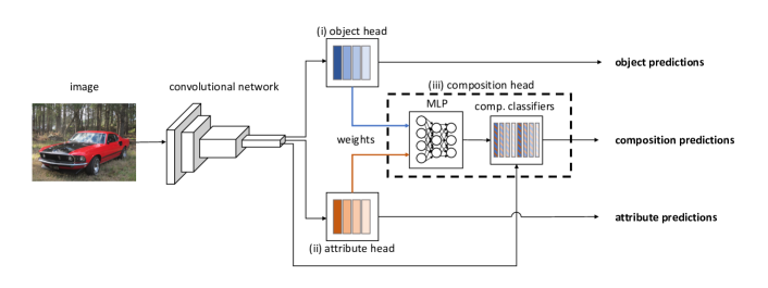
Figure 2. CompNet: Our proposed architecture with three output streams: (i) object predictions; (ii) object-agnostic attribute predictions; and, (iii) attribute-object composition predictions. Composition head takes individual object and attribute classifier weights as inputs and produces a composition classifier for each pair, which is then applied to image features.

3.2. Pipeline Architecture

Our CompNet pipeline consists of a convolutional neural network feature generator, followed by three heads, one for each task: object, attribute, and composition classification. An overview of the pipeline is depicted in Figure 2. Object and attribute heads are both single fully-connected layers, trained on their respective hashtag sets, i.e., objects and attributes. The score of the attributes ($s_{a}$) and objects ($s_{b}$) is computed as the dot product between the image features and the linear classifiers.

Composition head.

We adopt the approach of Misra et al. (Misra et al., 2017) to compose complex visual classifiers from two classifiers of different types (attribute and object). For example, given the classifier weights of attribute #red and object #car, this method outputs classifier weights for their composition #red_car (cf. Figure 2.)

Let $\bm{w}_{a}$ and $\bm{w}_{o}$ denote the $D$-dimensional linear classifier vectors for attribute $a$ and object $o$, that are applied to the $D$-dimensional image features $\phi(I)$ extracted from a Convolutional Neural Network (CNN) . Next, let us denote set of all attributes as $\mathcal{A}$, and all objects as $\mathcal{O}$. Attribute-object pairs are composed into the composition $ao$, or more precisely, their classifier vectors $\bm{w}_{a}$ and $\bm{w}_{o}$ are composed into the composition classifier vector $\bm{w}_{ao}$ of the same size. The composition is performed by feeding a concatenated pair of vectors $(\bm{w}_{a},\bm{w}_{o})$ into the multi-layer perceptron (MLP) that outputs a vector $\bm{w}_{ao}$. Formally, for each $a\in\mathcal{A}$ and each $o\in\mathcal{O}$, the classifier for composition $ao$ is computed as

(1) $$\bm{w}_{ao}=\mathscr{C}(\bm{w}_{a},\bm{w}_{o}),$$

where $\mathscr{C}$ is a composition function parameterized with an MLP and learned from our training data. Finally, $\bm{w}_{ao}$ is applied on the image feature $\phi(I)$,

(2) $$s_{ao}=\bm{w}_{ao}\cdot\phi(I),$$

where $\cdot$ denotes the dot-product and $s_{ao}$ is the attribute-object logit.

We now discuss how we diverge from Misra et al. (Misra et al., 2017), by proposing a novel composition loss function better suited for the weakly-supervised scenario (see Section 3.3), and the strategy for efficient inference in large attribute-object spaces (see Section 3.4).

3.3. Loss Functions

Our pipeline unifies three tasks into a single architecture: object, attribute, and composition classification. The final loss is a weighted sum of loss functions for each task:

$$L(I,y_{a},y_{o};\phi,\bm{w}_{a},\bm{w}_{o},\mathscr{C}) =\lambda_{a}L_{a}\left(s_{a},\;y_{a}\right)+\lambda_{o}L_{o}\left(s_{o},\;y_{o}\right)+$$

(3) $$\hskip 28.45274pt+\lambda_{ao}L_{ao}\left(s_{ao},\;y_{a}\wedge y_{o}\right),$$

where $y_{a}$ and $y_{o}$ are attribute and object labels, respectively.

3.3.1. Object and attribute loss

For the object and attribute loss functions ($L_{o}$ and $L_{a}$, respectively) we use the standard cross-entropy loss (Goodfellow et al., 2016) adjusted for the multi-label scenario (Mahajan et al., 2018), after applying softmax to the output. The multi-label adjustment is needed because images often contain multiple object and attribute hashtags. Each positive target is set to be $1/k$, where $k\geq 1$ corresponds to the number of hashtags from that specific task (object or attribute).

3.3.2. Composition loss

In (Misra et al., 2017), the authors propose to use the binary cross-entropy loss, after applying a sigmoid on the logit output from (2), in order to get a probability score:

$$p_{ao} =\text{sigmoid}(s_{ao}),$$

(4) $$L_{ao} =y_{ao}\log(p_{ao})+(1-y_{ao})\log(1-p_{ao}),$$

where the label $y_{ao}$ is $1$ only if the image has the composition $ao$ present, i.e. $y_{a}=1\wedge y_{o}=1$. Unfortunately, in our experiments, we obtained results that are significantly worse than a simple Softmax Product baseline (discussed in Section 4). We believe this is due to training with incomplete noisy annotation, consisting of weak positive labels and no negative ones. These findings coincide with observations in other weakly-supervised approaches exploring binary cross-entropy (Joulin et al., 2016; Sun et al., 2017; Mahajan et al., 2018).

However, naively applying a softmax on all compositions, as we did for the individual objects and attributes, is prohibitively expensive, as we have millions of compositions in our larger training dataset, or hundreds of thousands if we consider only those that have at least 100 occurrences. The computation cost is not only in back-propagating the loss across all compositions, but also due to the computation of composition classifiers. Instead, we rely on an efficient softmax approximation. Contrary to previous approximations, that e.g. simply update the classes present in the training batch (Joulin et al., 2016), we leverage the scores of the individual object and attribute scores to construct the set of hard negative classes.

Hard negative composition classes.

Let us define probability of attribute $a$ as $p_{a}$, and of object $o$ as $p_{o}$, which we obtain as the softmax output of individual object and attribute heads of the pipeline. Additionally, let us define a set of compositions present in the training set (seen only) as $\mathcal{C}^{\text{seen}}$. For each image, we find a set of $k$ negatives $\mathcal{N}$ to be used in softmax computation,

(5) $$\mathcal{N}=\operatorname*{arg\,kmax}_{a^{\prime}o^{\prime}\in\mathcal{C}^{\text{seen}}\setminus\{ao\in I\}}(p_{a^{\prime}}p_{o^{\prime}}),$$

where $\{ao\in I\}$ represent all the positive compositions for the image, computed as the Cartesian product of the positive object and positive attributes.

In other words, hard negatives are chosen for each image based on the individual softmax probability product, which is an approximation of the joint attribute and object probability. Next, we compute the composition classifiers for each positive $ao$ and the set of negatives $\mathcal{N}$, and get the logit scores after applying them to the image features, respectively $s_{ao}$ and $\mathcal{S}_{ao}^{\mathcal{N}}$.

The approximate softmax joint attribute-object probability for a composition $ao$ is now:

(6) $$p_{ao}=\text{softmax}_{ao}\left(\{s_{ao}\}\cup\mathcal{S}_{ao}^{\mathcal{N}}\right),$$

where $\text{softmax}_{ao}$ denotes the value associated with $ao$ in the softmax vector. Note that, in a naive approximation of the softmax, one would use entire space of compositions $\mathcal{C}$ to select hard negatives, instead of only using seen ones $\mathcal{C}^{\text{seen}}$ as in (5). Given that the majority of the compositions are actually not present in the training data, the unseen ones are often selected as negatives (never as positives). We observe drastically worsened performance on unseen compositions in that case, see ablation in Section 4.2 for details.

Conditional probability term.

When searching for hard negative compositions in the weakly-supervised setup, false negatives are often selected. To alleviate this, we additionally use the conditional rule to approximate the joint probability. As an example, if the positive composition is #red_dress, there is a high probability that other #red objects are negative examples for that image (e.g., #red_car and #red_chair), so we compute the joint attribute-object probability through the conditional probability of the object given attribute. Formally:

(7) $$p_{ao}^{a}=p_{a}\text{softmax}_{ao}\left(\left\{s_{a^{\prime}o^{\prime}}\mid a^{\prime}=a\land o^{\prime}\in\mathcal{O}\right\}\right).$$

Similarly, we can compute $p_{ao}^{o}$ through conditional probability of the attribute given object.

The final composition loss now becomes

(8) $$L_{ao}=-\left(\log(p_{ao})+\log(p_{ao}^{a})+\log(p_{ao}^{o})\right).$$

A simplified illustration of this procedure is depicted in Figure 3.

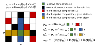
Figure 3. Illustration of our proposed composition loss. Joint attribute-object probability is approximated using hard negatives of the entire composition space, and through conditional probabilities, i.e., by fixing attribute and object class.

It is worth mentioning that there is often more than one positive composition per image. In fact, each pairwise combination of positive object and attribute hashtags is assumed to be a positive composition. We additionally use a multi-label version of the loss by weighting each positive label contribution to the loss with $1/k$, where $k\geq 1$ is the number of all pairwise combinations of attribute-object hashtags present in the image. A step-by-step procedure for the loss computation is summarized in Algorithm 1.

input:

     – batch of images $B$

     – feature generator $\phi$

     – object classifiers $\left\{\bm{w}_{o}^{\prime}\mid o^{\prime}\in\mathcal{O}\right\}$

     – attribute classifiers $\left\{\bm{w}_{a}^{\prime}\mid a^{\prime}\in\mathcal{A}\right\}$

     – composition MLP network $\mathscr{C}$

     – object and attribute #hashtags

for each image $I$ in $B$ do

       – compute loss for object and attribute head (Sec. 3.3.1)

       // we use $p_{a}$ and $p_{o}$ from prev. step for the following

       – select hard negative compositions (Eq. 5)

       – compute approx. composition probability $p_{ao}$ (Eq. 6)

       – compute approx. comp. probability $p_{ao}^{a}$ and $p_{ao}^{o}$ (Eq. 7)

       – compute composition loss using $p_{ao}$, $p_{ao}^{a}$, $p_{ao}^{o}$ (Eq. 8)

       – final loss is a weighted sum of three losses (Eq. 3.3)

      

end for

Algorithm 1 CompNet loss computation.

3.4. Inference

Outputting all possible composition scores for each image is computationally expensive, even at inference. In (Misra et al., 2017) scores are computed only for a predefined set of unseen compositions. Practically, this is unrealistic, as we do not have an oracle to decide which compositions will be useful at inference. More realistically, in (Nagarajan and Grauman, 2018) scores are computed for a larger predefined set of seen and unseen compositions. However, that still leaves out the majority of compositions, which simplifies inference, and diverges from realistically deployed system. In our setup, we do not assume any predefined set of compositions and propose a simple inference strategy: compute composition scores on a shortlist, consisting of every pairwise combination of top-$k_{a}$ attributes and top-$k_{o}$ objects predicted by attribute and object classifiers individually. Thus, the final composition logit output will have $k_{a}\times k_{o}$ entries, and the probabilities are computed by applying a softmax on these logits. If the composition being evaluated is not present in this shortlist, its probability is considered as 0 for the performance computation.

Table 1. Training implementation details. GPUs: total number of GPUs across machines with 8 GPUs per machine; Batch: total batch size, each GPU processes 32 images at a time and batch normalization (BN) (Ioffe and Szegedy, 2015) statistics are computed on these 32 image sets; Warm-up: to set the learning rate, we follow the linear scaling rule with gradual warm-up (Goyal et al., 2017) during the first X% of training iterations; LR init: learning rate initialization, this number is additionally multiplied with the total batch size.

Dataset	GPUs	Batch	Epochs	Warm-up	LR init	LR schedule	$\left[\lambda_{a},\lambda_{o},\lambda_{ao}\right]$	$|\mathcal{N}|$	top-$k_{a}{\times}k_{o}$
IG-8k-1k	128	4096	40	5% linear	0.1/256	${\times}$0.5 in 10 steps	$\left[1,1,1\right]$	10000	100${\times}$100
IG-504-144	128	4096	60	5% linear	0.1/256	${\times}$0.5 in 10 steps	$\left[1,1,1\right]$	5000	50${\times}$50
Marketplace	128	4096	32	12.5% linear	0.001/256	cosine (Loshchilov and Hutter, 2016)	$\left[1,1,10\right]$	all seen	100${\times}$100

4. Experiments

In this section we discuss implementation details, study different components of our method, and compare to the baselines.

4.1. Training and evaluation setup

Composition head details.

The function $\mathscr{C}$ is parametrized as a feed-forward multi-layer perceptron (MLP) with 2 hidden layers and a dropout (Srivastava et al., 2014) rate of $0.3$. Following (Misra et al., 2017), we use leaky ReLU (Maas et al., 2013) with coefficient $a=0.1$. The input to the MLP is a $2D$ dimensional vector constructed by concatenation of the attribute and object classifiers. Both hidden layers are $D$ dimensional and the final output is a $D$ dimensional attribute-object classifier.

Instagram details.

We use a ResNeXt-101 $32{\times}4$ (Xie et al., 2017) network trained from scratch by synchronous stochastic gradient descent (SGD). The final hyper-parameters are detailed in Table 1, and used throughout the experiments unless explicitly stated. Training on IG-8k-1k 78M images for 60 epochs took ${\sim}15$ days. Object and attribute tasks are evaluated using precision@1 (P@1), i.e., the percentage of images for which the top-scoring prediction is correct. Attribute-object pairs are evaluated using mean average precision (mAP), i.e., for each composition, rank all images and compute average precision, averaged across seen (S) and unseen (U) composition splits separately. We would like to point out that unlike many previous approaches, we do not have separate test data for seen and unseen compositions. This makes the unseen evaluation more challenging since training is biased towards seen attribute-object pairs. However, this mimicks the realistic deployment scenario where we can not distinguish between the seen and unseen attribute-object pairs.

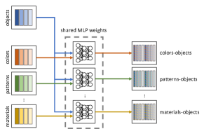
Figure 4. Composing classifiers for Marketplace. Each attribute type is composed with objects separately to generate 22 attribute-object heads with different attribute types.

Marketplace details.

We build on top of a previous system that was trained on our internal Marketplace attributes dataset. The trunk of the pipeline is a ResNet-50 (He et al., 2016) pre-trained on hashtags following (Mahajan et al., 2018). Attributes are split into 22 types, and a separate head is trained for each type. We extend the pipeline by adding an object category head with the 992 products, and combine it with each of the 22 attribute heads to create 22 composition heads, all of them sharing their weights, see Figure 4. The final hyper-parameters are detailed in Table 1. Due to the multi-head nature of attributes for this dataset, hard-negatives are selected for each attribute type separately. Object performance is evaluated using P@1, while attribute and composition performance using mAP.

4.2. Model study

Table 2. Model study of our proposed CompNet method. Performance is reported as mAP averaged over seen (S) and unseen (U) composition classes from IG-504-144.

	CompNet	IG-504-144
		S	U
(i)	vanilla softmax approximation	18.6	5.3
(ii)	remove unseen from hard negatives	19.1	10.3
(iii)	add conditional probability terms	19.3	11.2

To understand the effect of different design choices we experiment on the IG-504-144 dataset. Table 2 shows the performance of our proposed composition approach, quantifying the benefits of our proposed modifications to the loss function. Row (i) shows the results with vanilla softmax approximation where we do not remove unseen compositions from the hard negatives and remove conditional probability terms (cf. Section 3.3.2). The model learns to output low scores for unseen compositions, as it only uses them as negatives at training. In row (ii) we remove such compositions from the hard negatives (Eq. (5)) and observe a significant improvement in the performance of unseen attribute-object pairs ($5.3$ vs. $10.3$). Finally, in row (iii) we add the conditional terms back (Eq. 8) and observe a further improvement of $0.9$ mAP. Note that for the seen attribute-object pairs our design choices achieve a moderate improvement of $0.7$ mAP ($18.6$ vs.$19.3$) compared to the $5.9$ mAP improvement ($5.3$ vs. $11.2$) for the unseen ones.

We evaluate the robustness of our pipeline to the choice of top-$k$ hard negatives (Eq. 5) during training, and to the choice of output size top-$k_{a}{\times}k_{o}$ (Section 3.4) during inference. Results are presented in Table 3 for unseen compositions. First let us consider each row. We observe that performance is robust to the number of hard negatives during training. There is less than $0.15$ mAP degradation when we increase the hard negatives from $900$ to using all seen compositions. Now let us consider each column where we increase the number of compositions evaluated during inference. We observe an improvement of around $0.9$ mAP from top-$30{\times}30$ to top-$100{\times}100$. This indicates that performance is more sensitive to the number of compositions during inference and signifies trade-off between performance and deployment constraints like storage and latency.

Table 3. Effect of the number of hard negatives for training (Train top-$k$), and the number of compositions selected for inference (Test top-$k_{a}{\times}k_{o}$) for unseen classes (mAP metric) on IG-504-144 dataset.

Test top-$k_{a}{\times}k_{o}$	Train top-$k$
	900	2500	5000	ALL
$k_{a}=30$; $k_{o}=30$	9.70	9.82	9.84	9.84
$k_{a}=50$; $k_{o}=50$	10.15	10.27	10.28	10.29
$k_{a}=100$; $k_{o}=100$	10.63	10.74	10.73	10.76

4.3. Comparison with baselines

Baselines.

First, let us describe two simple baselines that are trained on the same data as our approach.

Composition FC. Instead of our composition head, we use a fully-connected (FC) layer to learn attribute-object classifiers directly. Note that only compositions observed at training can be learned using this approach. Hence, it is impossible to evaluate it on the unseen set. However, this method is still useful as an upper bound for composing classifiers on the seen attribute-object pairs. We only learn it on the smaller IG-504-144 dataset, where the number of compositions available at training is feasible.

Softmax Product. In this baseline, the composition head is removed from the pipeline, and a late fusion of individual attribute and object scores is performed. More precisely, joint attribute-object probability is estimated as a product of softmax probabilities from the attribute and object head of the system, i.e., $p_{ao}=p_{a}p_{o}$.

Instagram Datasets.

We compare CompNet pipeline against the baselines on Instagram datasets. There is a small but consistent performance improvement on standard object and attribute tasks, see Table 4. We attribute this to the fact that our composition head also benefits the image representation that is being trained jointly.

Table 5 shows the performance of different approaches on both seen and unseen attribute-object pairs. Our approach shows significant improvement over the Softmax Product baseline. This is especially prominent in the unseen case, where mAP improvement is $+4.0$ and $+3.9$ on IG-504-144 and IG-8k-1k, respectively. Additionally, as we increase the data scale, the gap between seen and unseen setup reduces significantly from $8.1$ mAP ($19.3$ (S), $11.2$ (U)) to $0.9$ mAP ($29.7$ (S), $28.8$ (U)). In contrast, note that the gap is $2.7$ mAP for Softmax Product baseline compared to $0.9$ with our approach for IG-8k-1k dataset. Finally, directly training linear classifiers on compositions (Composition FC) is just slightly better ($+0.3$ mAP) than our approach. This additionally amplifies the benefit of using composition network, which also generalizes to attribute-object pairs with no training data.

Table 4. Performance evaluation via precision@1 of the object and attribute heads on Instagram datasets.

Method	IG-504-144		IG-8k-1k
	Obj.	Attr.	Obj.	Attr.
Composition FC	70.9	29.9	–	–
Softmax Product	70.4	29.9	38.6	31.4
CompNet	71.0	30.0	38.9	31.7

Table 5. Performance evaluation of the composition head on Instagram datasets. Performance is reported as mAP averaged over seen (S) and unseen (U) composition splits.

Method	IG-504-144		IG-8k-1k
	S	U	S	U
Composition FC	19.6	–	–	–
Softmax Product	18.2	7.2	27.6	24.9
CompNet	19.3	11.2	29.7	28.8

Marketplace Datasets.

Similar observations are made when evaluating pipeline on our internal Marketplace dataset, see Table 6. We see significant improvements in both seen and unseen scenarios. This indicates the consistency of our evaluation and results between the weakly-supervised and fully-supervised settings.

Table 6. Performance evaluation of the entire framework (object, attribute, and, composition head) on Marketplace dataset. Performance is reported as precision@1 for objects, mAP for attributes, and, mAP averaged over seen (S) and unseen (U) composition splits.

Method	Object	Attribute	Compositions
			seen	unseen
Softmax Prod.	95.9	55.1	47.5	41.9
CompNet	96.0	56.4	50.1	46.9

Effect of Number of Training Epochs.

Figure 5 shows the results on seen and unseen compositions as we increase the number of training epochs for IG-8k-1k dataset. Note that, the plots do not present one training run evaluated at different stages of training. Rather, learning rate decay schedule is completed in full for each point on the plot. We observe that Softmax Product saturates or starts overfitting to seen compositions very early, i.e., after $20$ epochs. On the other hand, our pipeline continues improving unseen categories for a longer number of epochs, which in turn helps tighten the gap between seen and unseen performance.

Figure 5. Evaluating overfitting to seen compositions on Instagram datasets for varying lengths of the training.

4.4. Qualitative results

We extract predictions on the YFCC100m dataset (Thomee et al., 2015) due to large number of images and a high variation of fine-grained classes, and because we cannot show images from Instagram or Marketplace. YFCC100m does not have composition annotations, so we randomly picked 50 unseen compositions and inspected image shortlist with highest composition prediction scores. We compare our CompNet method with Softmax Product baseline, both trained on IG-8k-1k, and did not find any composition in which Softmax Product performed better. Few example compositions are depicted in Figure 6.

neon cat
CompNet  
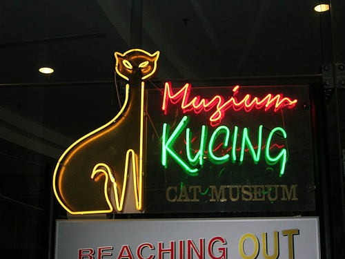
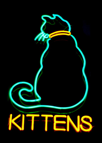
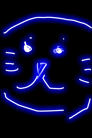
Softmax Prod.  
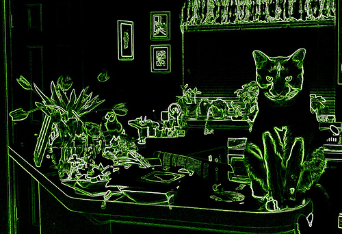
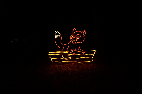
heart beach
CompNet  
Softmax Prod.  
charcoal apple
CompNet  
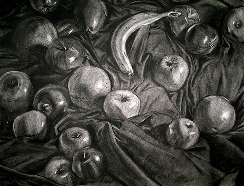
Softmax Prod.  
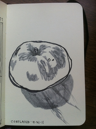
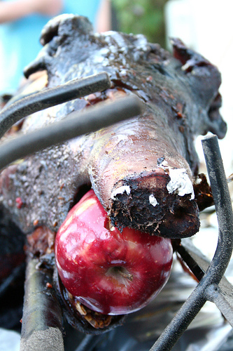
rope bridge
CompNet  
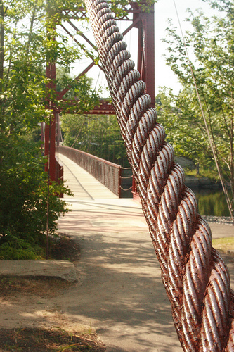
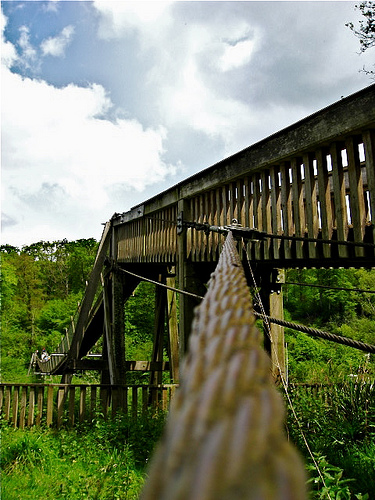
Softmax Prod.  

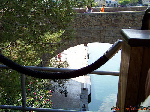
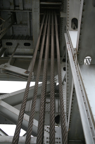
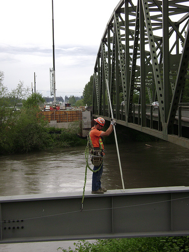
Figure 6. Qualitative comparison between our proposed CompNet (upper row) and Softmax Product (lower row) on unseen compositions from images of YFCC100m. Every $10^{th}$ ranked image is shown to capture a larger ranking.

5. Deployment

CompNet hasn’t been deployed at Facebook yet, but we have identified the first few large scale use-cases within Facebook Marketplace and have run experiments on the Marketplace data to verify the effectiveness of this approach for applications in Commerce.

5.1. Sample Use Cases

Marketplace Attributes Filters.

Users on Marketplace have access to filters which enable them to search items for the presence of a specific attribute within a category page. For instance, searching for products with the red color within the Women’s Dresses category. A major limitation to the currently deployed system is that the model predicts category specific attributes (red dress, peplum sweater, etc), each being learnt as a linear classifier, thus restricting the attributes to certain handpicked categories. So, adding a new category requires getting annotations for each applicable attribute. With CompNet, we can extend the set of categories to thousands without requiring new annotations because the attributes head is category agnostic. Hence, at inference time we could compose new attributes for unseen categories for free. This will enable us in increasing the coverage of attributes over the total inventory and adding new attributes filters which were not possible before.

Marketplace Browse Feed Ranking.

Browse Feed Ranking is a system that ranks the products on the homepage for all Marketplace users. The current ranking system uses a variety of features from multiple sources (user, image, and text). Our hypothesis is that having features related to fine-grained attributes on an image will help rank products better for every individual user. However, with handpicked categories, coverage is again an issue. With CompNet, we will be able to predict attributes over multiple categories (seen and unseen), thus improving the overall coverage, which might lead to downstream gains in ranking.

5.2. Deployment Challenges & Plan

There are some challenges in deploying the CompNet system in production from a compute and storage point of view. We decide not to use the MLP during inference and directly deploy the linear compositional classifiers so that the inference system is agnostic to the type of head used to construct the classifiers and simplify future upgrades. Assuming that CompNet predicts 1000 categories and 1000 attributes during inference, we have around 1M classifiers for the compositions. But, we do not need to deploy all 1M classifiers as from our past knowledge, we know that some attributes never occur with some categories (e.g. neckline attributes never occur with Home & Garden categories). So, we can significantly reduce the number of classifiers that we need to store at all times (in the order of few hundred of thousands or potentially even less). Hence, based on the inference strategy mentioned in Section 3.4, we load the top $k_{a}\times k_{o}$ classifiers out of the few hundreds of thousands deployed classifiers and compute scores.

After CompNet predictions are available during inference, we’ll store the outputs in a distributed key-value store, which would be consumed by multiple product groups. We go a step further and store only the top few (~100) compositional scores instead of $k_{a}\times k_{o}$ in permanent storage for consumption.

6. Conclusion and Future Work

In this work we explored a framework for joint attribute-object composition classification, learned from a large-scale weakly-supervised dataset, combining 8k objects and 1k attributes. Carefully designed loss functions enable us to handle noisy labels and generalize to compositions not present in the training data. Extensive evaluations show the benefits of using such an approach compared to a late fusion of individual attribute and object predictions.

There are few challenges we leave for future research. Namely, for a given image, training compositions are selected as every pairwise combination of attribute and object hashtags. When there is more than one attribute and/or more than one object, combining all of them will likely add noise. We plan on exploring weak localization techniques to alleviate this problem. Additionally, some attributes commonly occur with a specific object, and sparsely with others. For example, #striped always occurs with #zebra, and sparsely with #shirt, #wall, #couch, thus being biased towards a specific object category. We have not quantified such bias, but are planning to do so in an attempt to develop methods that reduce it.

References

- (1)
- Al-Halah et al. (2016) Ziad Al-Halah, Makarand Tapaswi, and Rainer Stiefelhagen. 2016. Recovering the missing link: Predicting class-attribute associations for unsupervised zero-shot learning. In CVPR.
- Baroni and Zamparelli (2010) Marco Baroni and Roberto Zamparelli. 2010. Nouns are vectors, adjectives are matrices: Representing adjective-noun constructions in semantic space. In EMNLP.
- Berg et al. (2010) Tamara L Berg, Alexander C Berg, and Jonathan Shih. 2010. Automatic attribute discovery and characterization from noisy web data. In ECCV.
- Chen and Grauman (2014) Chao-Yeh Chen and Kristen Grauman. 2014. Inferring analogous attributes. In CVPR.
- Chen et al. (2012) Huizhong Chen, Andrew Gallagher, and Bernd Girod. 2012. Describing clothing by semantic attributes. In ECCV.
- Chen et al. (2020) Hui Chen, Zhixiong Nan, Jiang Jingjing, and Nanning Zheng. 2020. Learning to Infer Unseen Attribute-Object Compositions. arXiv:2010.14343 (2020).
- Deng et al. (2014) Yubin Deng, Ping Luo, Chen Change Loy, and Xiaoou Tang. 2014. Pedestrian attribute recognition at far distance. In ACM-MM.
- Denton et al. (2015) Emily Denton, Jason Weston, Manohar Paluri, Lubomir Bourdev, and Rob Fergus. 2015. User conditional hashtag prediction for images. In SIGKDD.
- Duan et al. (2012) Kun Duan, Devi Parikh, David Crandall, and Kristen Grauman. 2012. Discovering localized attributes for fine-grained recognition. In CVPR.
- Farhadi et al. (2009) Ali Farhadi, Ian Endres, Derek Hoiem, and David Forsyth. 2009. Describing objects by their attributes. In CVPR.
- Georgopoulos et al. (2020) Markos Georgopoulos, Grigorios Chrysos, Maja Pantic, and Yannis Panagakis. 2020. Multilinear Latent Conditioning for Generating Unseen Attribute Combinations. In ICML.
- Goodfellow et al. (2016) Ian Goodfellow, Yoshua Bengio, and Aaron Courville. 2016. Deep learning. MIT press Cambridge.
- Goyal et al. (2017) Priya Goyal, Piotr Dollár, Ross Girshick, Pieter Noordhuis, Lukasz Wesolowski, Aapo Kyrola, Andrew Tulloch, Yangqing Jia, and Kaiming He. 2017. Accurate, large minibatch sgd: Training imagenet in 1 hour. arXiv:1706.02677 (2017).
- Gross et al. (2017) Sam Gross, Marc’Aurelio Ranzato, and Arthur Szlam. 2017. Hard mixtures of experts for large scale weakly supervised vision. In CVPR.
- Guevara (2010) Emiliano Raul Guevara. 2010. A regression model of adjective-noun compositionality in distributional semantics. In GEMS.
- He et al. (2016) Kaiming He, Xiangyu Zhang, Shaoqing Ren, and Jian Sun. 2016. Deep residual learning for image recognition. In CVPR.
- Hsiao and Grauman (2017) Wei-Lin Hsiao and Kristen Grauman. 2017. Learning the latent ”look”: Unsupervised discovery of a style-coherent embedding from fashion images. In ICCV.
- Ioffe and Szegedy (2015) Sergey Ioffe and Christian Szegedy. 2015. Batch normalization: Accelerating deep network training by reducing internal covariate shift. arXiv:1502.03167 (2015).
- Isola et al. (2015) Phillip Isola, Joseph J Lim, and Edward H Adelson. 2015. Discovering states and transformations in image collections. In CVPR.
- Joulin et al. (2016) Armand Joulin, Laurens Van Der Maaten, Allan Jabri, and Nicolas Vasilache. 2016. Learning visual features from large weakly supervised data. In ECCV.
- Kovashka et al. (2012) Adriana Kovashka, Devi Parikh, and Kristen Grauman. 2012. Whittlesearch: Image search with relative attribute feedback. In CVPR.
- Krizhevsky et al. (2012) Alex Krizhevsky, Ilya Sutskever, and Geoffrey E Hinton. 2012. Imagenet classification with deep convolutional neural networks. In NeurIPS.
- Kumar et al. (2008) Neeraj Kumar, Peter Belhumeur, and Shree Nayar. 2008. Facetracer: A search engine for large collections of images with faces. In ECCV.
- Kumar et al. (2011) Neeraj Kumar, Alexander Berg, Peter N Belhumeur, and Shree Nayar. 2011. Describable visual attributes for face verification and image search. TPAMI (2011).
- Kumar et al. (2009) Neeraj Kumar, Alexander C Berg, Peter N Belhumeur, and Shree K Nayar. 2009. Attribute and simile classifiers for face verification. In ICCV.
- Laffont et al. (2014) Pierre-Yves Laffont, Zhile Ren, Xiaofeng Tao, Chao Qian, and James Hays. 2014. Transient attributes for high-level understanding and editing of outdoor scenes. TOG (2014).
- Lampert et al. (2009) Christoph H Lampert, Hannes Nickisch, and Stefan Harmeling. 2009. Learning to detect unseen object classes by between-class attribute transfer. In CVPR.
- Li et al. (2017) Ang Li, Allan Jabri, Armand Joulin, and Laurens van der Maaten. 2017. Learning visual n-grams from web data. In ICCV.
- Liu et al. (2011) Jingen Liu, Benjamin Kuipers, and Silvio Savarese. 2011. Recognizing human actions by attributes. In CVPR.
- Liu et al. (2016) Ziwei Liu, Ping Luo, Shi Qiu, Xiaogang Wang, and Xiaoou Tang. 2016. DeepFashion: Powering Robust Clothes Recognition and Retrieval with Rich Annotations. In CVPR.
- Liu et al. (2015) Ziwei Liu, Ping Luo, Xiaogang Wang, and Xiaoou Tang. 2015. Deep learning face attributes in the wild. In ICCV.
- Loshchilov and Hutter (2016) Ilya Loshchilov and Frank Hutter. 2016. Sgdr: Stochastic gradient descent with warm restarts. arXiv:1608.03983 (2016).
- Lu et al. (2017) Yongxi Lu, Abhishek Kumar, Shuangfei Zhai, Yu Cheng, Tara Javidi, and Rogerio Feris. 2017. Fully-adaptive feature sharing in multi-task networks with applications in person attribute classification. In CVPR.
- Maas et al. (2013) Andrew L Maas, Awni Y Hannun, and Andrew Y Ng. 2013. Rectifier nonlinearities improve neural network acoustic models. In ICML.
- Mahajan et al. (2018) Dhruv Mahajan, Ross Girshick, Vignesh Ramanathan, Kaiming He, Manohar Paluri, Yixuan Li, Ashwin Bharambe, and Laurens van der Maaten. 2018. Exploring the limits of weakly supervised pretraining. In ECCV.
- Miller (1995) George A Miller. 1995. WordNet: a lexical database for English. Commun. ACM (1995).
- Misra et al. (2017) Ishan Misra, Abhinav Gupta, and Martial Hebert. 2017. From red wine to red tomato: Composition with context. In CVPR.
- Mitchell and Lapata (2008) Jeff Mitchell and Mirella Lapata. 2008. Vector-based models of semantic composition. In ACL-HLT.
- Nagarajan and Grauman (2018) Tushar Nagarajan and Kristen Grauman. 2018. Attributes as operators: factorizing unseen attribute-object compositions. In ECCV.
- Nguyen et al. (2014) Dat Tien Nguyen, Angeliki Lazaridou, and Raffaella Bernardi. 2014. Coloring objects: adjective-noun visual semantic compositionality. In ACL Workshop on Vision and Language.
- Patterson and Hays (2012) Genevieve Patterson and James Hays. 2012. Sun attribute database: Discovering, annotating, and recognizing scene attributes. In CVPR.
- Patterson and Hays (2016) Genevieve Patterson and James Hays. 2016. Coco attributes: Attributes for people, animals, and objects. In ECCV.
- Pezzelle et al. (2016) Sandro Pezzelle, Ravi Shekhar, and Raffaella Bernardi. 2016. Building a bagpipe with a bag and a pipe: Exploring conceptual combination in vision. In ACL Workshop on Vision and Language.
- Russakovsky et al. (2015) Olga Russakovsky, Jia Deng, Hao Su, Jonathan Krause, Sanjeev Satheesh, Sean Ma, Zhiheng Huang, Andrej Karpathy, Aditya Khosla, Michael Bernstein, et al. 2015. Imagenet large scale visual recognition challenge. IJCV (2015).
- Russakovsky and Fei-Fei (2010) Olga Russakovsky and Li Fei-Fei. 2010. Attribute learning in large-scale datasets. In ECCV.
- Sadeghi and Farhadi (2011) Mohammad Amin Sadeghi and Ali Farhadi. 2011. Recognition using visual phrases. In CVPR.
- Santa Cruz et al. (2018) Rodrigo Santa Cruz, Basura Fernando, Anoop Cherian, and Stephen Gould. 2018. Neural algebra of classifiers. In WACV.
- Sharma and Jurie (2011) Gaurav Sharma and Frederic Jurie. 2011. Learning discriminative spatial representation for image classification. In BMVC.
- Singh and Lee (2016) Krishna Kumar Singh and Yong Jae Lee. 2016. End-to-end localization and ranking for relative attributes. In ECCV.
- Socher et al. (2013) Richard Socher, Alex Perelygin, Jean Wu, Jason Chuang, Christopher D Manning, Andrew Y Ng, and Christopher Potts. 2013. Recursive deep models for semantic compositionality over a sentiment treebank. In EMNLP.
- Srivastava et al. (2014) Nitish Srivastava, Geoffrey Hinton, Alex Krizhevsky, Ilya Sutskever, and Ruslan Salakhutdinov. 2014. Dropout: a simple way to prevent neural networks from overfitting. JMLR (2014).
- Su et al. (2016) Chi Su, Shiliang Zhang, Junliang Xing, Wen Gao, and Qi Tian. 2016. Deep attributes driven multi-camera person re-identification. In ECCV.
- Sun et al. (2017) Chen Sun, Abhinav Shrivastava, Saurabh Singh, and Abhinav Gupta. 2017. Revisiting unreasonable effectiveness of data in deep learning era. In ICCV.
- Thomee et al. (2015) Bart Thomee, David A Shamma, Gerald Friedland, Benjamin Elizalde, Karl Ni, Douglas Poland, Damian Borth, and Li-Jia Li. 2015. The new data and new challenges in multimedia research. arXiv:1503.01817 (2015).
- Veit et al. (2018) Andreas Veit, Maximilian Nickel, Serge Belongie, and Laurens van der Maaten. 2018. Separating self-expression and visual content in hashtag supervision. In CVPR.
- Wang et al. (2016) Jing Wang, Yu Cheng, and Rogerio Schmidt Feris. 2016. Walk and learn: Facial attribute representation learning from egocentric video and contextual data. In CVPR.
- Wang et al. (2019) Xiao Wang, Shaofei Zheng, Rui Yang, Bin Luo, and Jin Tang. 2019. Pedestrian attribute recognition: A survey. arXiv:1901.07474 (2019).
- Xie et al. (2017) Saining Xie, Ross Girshick, Piotr Dollár, Zhuowen Tu, and Kaiming He. 2017. Aggregated residual transformations for deep neural networks. In CVPR.
- Yan et al. (2016) Xinchen Yan, Jimei Yang, Kihyuk Sohn, and Honglak Lee. 2016. Attribute2image: Conditional image generation from visual attributes. In ECCV.
- Yu and Grauman (2014) Aron Yu and Kristen Grauman. 2014. Fine-grained visual comparisons with local learning. In CVPR.
- Zhang et al. (2017) Hanwang Zhang, Zawlin Kyaw, Shih-Fu Chang, and Tat-Seng Chua. 2017. Visual translation embedding network for visual relation detection. In CVPR.
- Zhao et al. (2019) Bo Zhao, Yanwei Fu, Rui Liang, Jiahong Wu, Yonggang Wang, and Yizhou Wang. 2019. A large-scale attribute dataset for zero-shot learning. In CVPRW.