On the pathwidth of hyperbolic 3-manifolds

Abstract

According to Mostow’s celebrated rigidity theorem, the geometry of closed hyperbolic 3-manifolds is already determined by their topology. In particular, the volume of such manifolds is a topological invariant and, as such, has been investigated for half a century.

Motivated by the algorithmic study of 3-manifolds, Maria and Purcell have recently shown that every closed hyperbolic 3-manifold $\mathcal{M}$ with volume $\operatorname{vol}(\mathcal{M})$ admits a triangulation with dual graph of treewidth at most $C\cdot\operatorname{vol}(\mathcal{M})$, for some universal constant $C$.

Here we improve on this result by showing that the volume provides a linear upper bound even on the pathwidth of the dual graph of some triangulation, which can potentially be much larger than the treewidth. Our proof relies on a synthesis of tools from 3-manifold theory: generalized Heegaard splittings, amalgamations, and the thick-thin decomposition of hyperbolic 3-manifolds. We provide an illustrated exposition of this toolbox and also discuss the algorithmic consequences of the result.

1 Introduction

Algorithms in computational 3-manifold topology typically take a triangulation as input and return topological information about the underlying manifold. The difficulty of extracting the desired information, however, might greatly depend on the choice of the input triangulation. In recent years, several computationally hard problems about triangulated 3-manifolds were shown to admit algorithmic solutions that are fixed-parameter tractable (FPT) in the treewidth of the dual graph of the input triangulation [12, 13, 14, 15, 16]. These algorithms still require exponential time to terminate in the worst case. However, for triangulations with dual graph of bounded treewidth they run in polynomial time.^,

In the light of these algorithms, it is compelling to consider the treewidth $\operatorname{tw}(\mathcal{M})$ of a compact $3$-manifold $\mathcal{M}$, defined as the smallest treewidth of the dual graph of any triangulation thereof. Over the last few years, the quantitative relationship between the treewidth and other properties of 3-manifolds has been studied in various settings. The author together with Spreer showed, for instance, that the Heegaard genus always gives an upper bound on the treewidth (even on the pathwidth) [25], and together with Wagner they established that, for certain families of 3-manifolds the treewidth can be arbitrary large [26].

Recently, Maria and Purcell have shown that, in the realm of hyperbolic 3-manifolds another important invariant, the volume, yields an upper bound on the treewidth [36]. They proved the existence of a universal constant $C>0$, such that, for every closed hyperbolic 3-manifold $\mathcal{M}$ with treewidth $\operatorname{tw}(\mathcal{M})$ and volume $\operatorname{vol}(\mathcal{M})$ the following inequality holds:

$$\operatorname{tw}(\mathcal{M})\leq C\cdot\operatorname{vol}(\mathcal{M}).$$ (1)

In this article we improve upon (1) by showing that the volume provides a linear upper bound even on the pathwidth of a hyperbolic 3-manifold—a quantity closely related to, but potentially much larger than the treewidth. More precisely, we prove the following theorem.

Theorem 1.

There exists a universal constant $C^{\prime}>0$ such that, for any closed, orientable and hyperbolic $3$-manifold $\mathcal{M}$ with pathwidth $\operatorname{pw}(\mathcal{M})$ and volume $\operatorname{vol}(\mathcal{M})$, we have

$$\operatorname{pw}(\mathcal{M})\leq C^{\prime}\cdot\operatorname{vol}(\mathcal{M}).$$ (2)

Outline of the proof.

Our roadmap to establish Theorem 1 is similar to that in [36]. In particular, our construction of a triangulation of $\mathcal{M}$ with dual graph of pathwidth bounded in terms of $\operatorname{vol}(\mathcal{M})$ also starts with a thick-thin decomposition $\mathscr{D}$ of $\mathcal{M}$. The two proofs, however, diverge at this point. Maria and Purcell proceed by triangulating the thick part of $\mathscr{D}$ using the work of Jørgensen–Thurston [60, §5.11] and Kobayashi–Rieck [33]. This partial triangulation is then simplified [9, 28] and completed into the desired triangulation of $\mathcal{M}$.

The novelty in our work is, that we proceed by first turning the decomposition $\mathscr{D}$ into a generalized Heegaard splitting of $\mathcal{M}$ [52, 53], where we rely on the aforementioned results to control the genera of the splitting surfaces. Next, we amalgamate this generalized Heegaard splitting into a classical one [54]. Finally, we appeal to our earlier work [25] to turn this Heegaard splitting into a triangulation of $\mathcal{M}$ with dual graph of pathwidth $O(\operatorname{vol}(\mathcal{M}))$.

The proof of Theorem 1 provides a template for an algorithm to triangulate any closed hyperbolic 3-manifold $\mathcal{M}$ in such a way, that the dual graph of the resulting triangulation has pathwidth $O(\operatorname{vol}(\mathcal{M}))$. Using such triangulations—that have a dual graph not only of small treewidth, but also pathwidth—as input for FPT-algorithms may significantly reduce their running time. This is because such triangulations lend themselves to nice tree decompositions (the data structure underlying many algorithms FPT in the treewidth) without join bags (those parts of a nice tree decomposition that often account for the computational bottleneck, cf. [13]). The upshot of Theorem 1 is that, in case of hyperbolic 3-manifolds with bounded volume working with such triangulations is (in theory) always possible.

Structure of the paper.

We start with an illustrated exposition of the various notions from 3-manifold theory we rely on (Section 2). Then, in Section 3, we discuss the treewidth and pathwidth for graphs and 3-manifolds alike. In Section 4, we put all the pieces together to prove Theorem 1. We conclude with a discussion and some open questions in Section 5.

Acknowledgements.

I am grateful to Uli Wagner and Jonathan Spreer for their guidance and steady support during my PhD, and Éric Colin de Verdière and Herbert Edelsbrunner for their careful review of my thesis. I thank the anonymous referees for their useful suggestions to improve the exposition. I also thank Clément Maria for many stimulating discussions, and my colleagues at Inria for the warm welcome in Sophia Antipolis in the midst of a pandemic.

2 A primer on 3-manifolds

The main objects of study in this paper are 3-dimensional manifolds, or $3$-manifolds for short. As we will also encounter 2-manifolds, also known as surfaces, we give the general definition. A $d$-dimensional manifold with boundary is a topological space $\mathcal{M}$ such that each point $x\in\mathcal{M}$ has a neighborhood which looks like (i.e., is homeomorphic to) the Euclidean $d$-space $\mathbb{R}^{d}$ or the closed upper half-space $\{(x_{1},\ldots,x_{d})\in\mathbb{R}^{d}:x_{d}\geq 0\}$. The points of $\mathcal{M}$ that do not have a neighborhood homeomorphic to $\mathbb{R}^{d}$ constitute the boundary $\partial\mathcal{M}$ of $\mathcal{M}$. A compact manifold is said to be closed if it has an empty boundary.

Two manifolds $\mathcal{M}_{1}$ and $\mathcal{M}_{2}$ are considered equivalent if they are homeomorphic, i.e., if there exists a continuous bijection $f\colon\mathcal{M}_{1}\rightarrow\mathcal{M}_{2}$ with $f^{-1}$ being continuous as well. Properties of manifolds that are preserved under homeomorphisms are called topological invariants. We refer to [55] for an introduction to 3-manifolds (cf. [23, 27, 50, 59]).

All $3$-manifolds in this paper are assumed to be compact and orientable.

2.1 Triangulations and handle decompositions

Triangulations.

By a classical result of Moise [40] (cf. [4]) every compact 3-manifold admits a triangulation. To build a triangulation, take a disjoint union $\widetilde{\Delta}=\Delta_{1}\cup\ldots\cup\Delta_{n}$ of finitely many tetrahedra with $4n$ triangular faces altogether. Let $\Phi=\{\varphi_{1},\ldots,\varphi_{m}\}$ be a set of at most $2n$ face gluings, each of which identifies a pair of these triangular faces in such a way that vertices are mapped to vertices, edges to edges, and each face is identified with at most one other face, see Figure 1(i). The resulting quotient space $\mathcal{T}=\widetilde{\Delta}/\Phi$ is called a triangulation, and the pairs of identified triangular faces are referred to as triangles of $\mathcal{T}$. Note that these face gluings might identify several tetrahedral edges (or vertices) of $\widetilde{\Delta}$ resulting in a single edge (or vertex) of $\mathcal{T}$.

To obtain a triangulation $\mathcal{T}$ that is homeomorphic to a closed $3$-manifold $\mathcal{M}$, it is necessary and sufficient that the boundary of a small neighborhood around each vertex is a sphere, and no edge is identified with itself in reverse. If some of the vertices have small neighborhoods with boundaries being disks, then $\mathcal{T}$ describes a $3$-manifold with boundary. In a computational setting, a 3-manifold is very often presented this way.

In the study of triangulations, their dual graphs play an instrumental role. Given a triangulation $\mathcal{T}=\widetilde{\Delta}/\Phi$, its dual graph $\Gamma(\mathcal{T})=(V,E)$ is a multigraph where the nodes in $V$ correspond to the tetrahedra in $\widetilde{\Delta}$, and for each face gluing $\varphi\in\Phi$ identifying two triangular faces of $\Delta_{i}$ and $\Delta_{j}$, we add an arc between the corresponding nodes in $V$, cf. Figure 1(ii). (Note that $i$ and $j$ could be equal.) By construction, every node of $\Gamma(\mathcal{T})$ has maximum degree $\leq 4$. Moreover, when $\mathcal{T}$ triangulates a closed 3-manifold, then $\Gamma(\mathcal{T})$ is 4-regular.

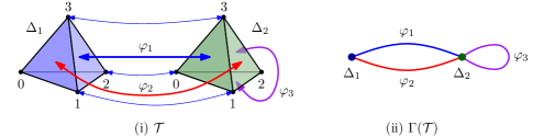
Figure 1: (i) A triangulation $\mathcal{T}=\widetilde{\Delta}/\Phi$ with two tetrahedra $\widetilde{\Delta}=\{\Delta_{1},\Delta_{2}\}$ and three face gluing maps $\Phi=\{\varphi_{1},\varphi_{2},\varphi_{3}\}.$ $\varphi_{1}$ is specified to be $\Delta_{1}(123)\overset{\displaystyle\varphi_{1}}{\longleftrightarrow}\Delta_{2}(103)$. (ii) The dual graph $\Gamma(\mathcal{T})$ of $\mathcal{T}$.

Handle decompositions.

It follows from Morse theory (and also from the existence of triangulations) that every compact $3$-manifold can be built from finitely many solid building blocks called $0$-, $1$-, $2$-, and $3$-handles. In such a handle decomposition all handles are homeomorphic to $3$-balls, and are only distinguished in how they are glued together. To construct a closed $3$-manifold from handles, we may start with a disjoint union of $3$-balls, or $0$-handles, where further $3$-balls are glued to the boundary of the existing decomposition along pairs of $2$-dimensional disks ($1$-handles), or along annuli ($2$-handles). This process is iterated until the boundary consists of a disjoint union of $2$-spheres. These are then eliminated by gluing in one $3$-ball per boundary component, the $3$-handles of the decomposition.

Figure 2: (i) A 0-handle, (ii) a 1-handle, (iii) a 2-handle, and (iv) a 3-handle. The attaching sites are indicated with light blue. For a 1-handle, this is a disjoint union of two disks, for a 2-handle an annulus, and for a 3-handle the entire 2-sphere boundary.

2.2 Handlebodies and compression bodies

A handlebody $\mathcal{H}$ is a connected $3$-manifold with boundary that is built from (finitely many) $0$-handles and $1$-handles. It can also be seen as a thickened graph. Up to homeomorphism, a handlebody $\mathcal{H}$ is determined by the genus $g(\partial\mathcal{H})$ of its boundary.

Let $\mathcal{S}$ be a compact, orientable (not necessarily connected) surface. A compression body is a $3$-manifold $\mathcal{C}$ obtained from $\mathcal{S}\times[0,1]$ by (optionally) attaching some $1$-handles to $\mathcal{S}\times\{1\}$, and (optionally) filling in some of the $2$-sphere components of $\mathcal{S}\times\{0\}$ with $3$-balls. $\mathcal{C}$ has two sets of boundary components: $\partial_{-}\mathcal{C}=\mathcal{S}\times\{0\}\setminus\{\text{filled-in 2-sphere components}\}$ and $\partial_{+}\mathcal{C}=\partial\mathcal{C}\setminus\partial_{-}\mathcal{C}$. We call $\partial_{+}\mathcal{C}$ the upper boundary, and $\partial_{-}\mathcal{C}$ the lower boundary of $\mathcal{C}$.

Dual to this construction, a compression body $\mathcal{C}$ can also be built by starting with a closed, orientable surface $\mathcal{F}$, thickening it to $\mathcal{F}\times[0,1]$, (optionally) attaching some $2$-handles along $\mathcal{F}\times\{0\}$, and (optionally) filling in some of the resulting $2$-spheres with $3$-balls. The upper and lower boundary are given by $\partial_{+}\mathcal{C}=\mathcal{F}\times\{1\}$ and $\partial_{-}\mathcal{C}=\partial\mathcal{C}\setminus\partial_{+}\mathcal{C}$.

Note that every handlebody is also a compression body, where all 2-sphere components are eliminated in the last step.

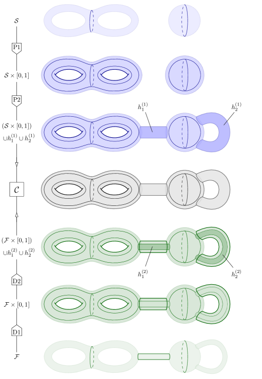
Figure 12: The primal and dual ways of constructing a compression body $\mathcal{C}$, cf. Section 2.2.

See Figure 12 in Appendix A for an illustration of the primal and dual constructions.

2.3 Heegaard splittings

Introduced in [22], Heegaard splittings have been central to the study of 3-manifolds for over a century. Given a closed, orientable 3-manifold $\mathcal{M}$, a Heegaard splitting is a decomposition $\mathcal{M}=\mathcal{H}\cup_{\mathcal{S}}\mathcal{H}^{\prime}$ where $\mathcal{H}$ and $\mathcal{H}^{\prime}$ are homeomorphic handlebodies with $\mathcal{H}\cup\mathcal{H}^{\prime}=\mathcal{M}$ and $\mathcal{H}\cap\mathcal{H}^{\prime}=\partial\mathcal{H}=\partial\mathcal{H}^{\prime}=\mathcal{S}$ called the splitting surface. The Heegaard genus $\mathfrak{g}\left(\mathcal{M}\right)$ of $\mathcal{M}$ is the smallest genus $g(\mathcal{S})$ over all Heegaard splittings of $\mathcal{M}.$ See [51] for a comprehensive survey.

Example 2 (Heegaard splittings from triangulations, I).

Given a triangulation $\mathcal{T}$ of a closed, orientable 3-manifold $\mathcal{M}$, let $\mathcal{T}^{(1)}$ denote its $1$-skeleton consisting of the vertices and edges of $\mathcal{T}$. Thickening up $\mathcal{T}^{(1)}$, i.e., taking its regular neighborhood, in $\mathcal{M}$ yields a handlebody $\mathcal{H}_{1}$. The closure $\mathcal{H}_{2}$ of the complement $\mathcal{M}\setminus\mathcal{H}_{1}$ is also a handlebody homeomorphic to a regular neighborhood of $\Gamma(\mathcal{T})$, and $\mathcal{M}=\mathcal{H}_{1}\cup\mathcal{H}_{2}$ is a Heegaard splitting of $\mathcal{M}$.

Heegaard splittings of 3-manifolds with boundary.

Using compression bodies, one can generalize Heegaard splittings to 3-manifolds with nonempty boundary. Let $\mathcal{M}$ be a $3$-manifold and $\partial_{1}\mathcal{M}\cup\partial_{2}\mathcal{M}=\partial\mathcal{M}$ be an arbitrary partition of its boundary components. There exist compression bodies $\mathcal{C}_{1}$ and $\mathcal{C}_{2}$ with $\mathcal{C}_{1}\cup\mathcal{C}_{2}=\mathcal{M}$, $\partial_{-}\mathcal{C}_{1}=\partial_{1}\mathcal{M}$, $\partial_{-}\mathcal{C}_{2}=\partial_{2}\mathcal{M}$, and $\mathcal{C}_{1}\cap\mathcal{C}_{2}=\partial_{+}\mathcal{C}_{1}=\partial_{+}\mathcal{C}_{2}$. The decomposition $\mathcal{M}=\mathcal{C}_{1}\cup_{\mathcal{S}}\mathcal{C}_{2}$ is called a Heegaard splitting of $\mathcal{M}$ compatible with the partition $\partial_{1}\mathcal{M}\cup\partial_{2}\mathcal{M}$. Its splitting surface is $\mathcal{S}=\mathcal{C}_{1}\cap\mathcal{C}_{2}$. The Heegaard genus $\mathfrak{g}\left(\mathcal{M}\right)$ is again the minimum genus $g(\mathcal{S})$ over all such decompositions.

See Example 16 in Appendix B for an extension of Example 2 to this setting.

2.4 Generalized Heegaard splittings

The notion of a Heegaard splitting, where a 3-manifold is built by gluing two handlebodies together (or two compression bodies, in case of 3-manifolds with boundary), was refined by Scharlemann and Thompson in a seminal paper [53]. In a generalized Heegaard splitting a 3-manifold is constructed from several pairs of compression bodies. This construction arises naturally, e.g., when a 3-manifold is assembled by first attaching only some of the $0$- and $1$-handles before attaching any $2$- and $3$-handles.

Informally, a generalized Heegaard splitting of a $3$-manifold $\mathcal{M}$ is a decomposition

$$\mathscr{D}=\left\{\mathcal{M}_{i}:i\in I,\leavevmode\nobreak\ \textstyle\bigcup_{i\in I}\mathcal{M}_{i}=\mathcal{M},\leavevmode\nobreak\ \text{and}\leavevmode\nobreak\ \operatorname{int}(\mathcal{M}_{i})\cap\operatorname{int}(\mathcal{M}_{j})=\emptyset\leavevmode\nobreak\ \text{for}\leavevmode\nobreak\ i\neq j\right\}$$ (3)

into finitely many $3$-manifolds with pairwise disjoint interiors that intersect along surfaces, together with an “appropriate” Heegaard splitting for each $\mathcal{M}_{i}$. We make this now precise.

Given a decomposition $\mathscr{D}$ as above, consider its dual graph, which is a multigraph $\Gamma(\mathscr{D})=(I,E)$ with nodes corresponding to the $\mathcal{M}_{i}$ and arcs between $i$ and $j$ to the connected components of $\mathcal{M}_{i}\cap\mathcal{M}_{j}$ (Figure 3). Pick an ordering of $I$, i.e., a bijection $\ell\colon I\rightarrow\{1,\ldots,|I|\}$. For any $i\in I$, let $\partial_{1}\mathcal{M}_{i}\cup\partial_{2}\mathcal{M}_{i}$ be a partition of the connected components of $\partial\mathcal{M}_{i}$ so that $\partial_{1}\mathcal{M}_{i}$ (resp. $\partial_{2}\mathcal{M}_{i}$) contains the components glued to those of any $\mathcal{M}_{j}$ with $\ell(j)<\ell(i)$ (resp. $\ell(j)>\ell(i)$). Those components of $\partial\mathcal{M}_{i}$ which contribute to the boundary of $\mathcal{M}$ are partitioned among $\partial_{1}\mathcal{M}_{i}$ and $\partial_{2}\mathcal{M}_{i}$ arbitrarily. For each $i\in I$, choose a Heegaard splitting $\mathcal{M}_{i}=\mathcal{N}_{i}\cup_{\mathcal{S}_{i}}\mathcal{K}_{i}$ of $\mathcal{M}_{i}$ compatible with the partition $\partial_{1}\mathcal{M}_{i}\cup\partial_{2}\mathcal{M}_{i}$ of the boundary components (cf. Example 16). We obtain a generalized Heegaard splitting of $\mathcal{M}$ (Figure 4).

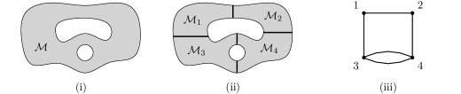
Figure 3: (i) Schematic of a closed 3-manifold $\mathcal{M}$ with nontrivial first homology, (ii) a decomposition $\mathscr{D}$ of $\mathcal{M}$ into four submanifolds, and (iii) the dual graph $\Gamma(\mathscr{D})$ of $\mathscr{D}$.

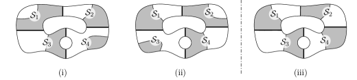
Figure 4: (i)–(ii) Schematics of two generalized Heegaard splittings of $\mathcal{M}$ stemming from the decomposition shown on Figure 3. These splittings respectively correspond to the orderings $\ell_{1}(i)=i$ ($i\in I=\{1,2,3,4\}$), and $\ell_{2}(1)=2$, $\ell_{2}(2)=4$, $\ell_{2}(3)=1$, $\ell_{2}(4)=3$. (iii) A non-example.

When we only need to talk about the constituents of a decomposition or the pieces of a generalized Heegaard splitting of a 3-manfiold $\mathcal{M}$ we use the shorthand notation

$$\mathcal{M}=\bigcup_{i\in I}\mathcal{M}_{i}\quad\text{or}\quad\mathcal{M}=\bigcup_{i\in I}(\mathcal{N}_{i}\cup_{\mathcal{S}_{i}}\mathcal{K}_{i}),\quad\text{where}\quad\mathcal{N}_{i}\cup_{\mathcal{S}_{i}}\mathcal{K}_{i}=\mathcal{M}_{i}.$$ (4)

Fork complexes.

When connectivity properties of the graph $\Gamma(\mathscr{D})$ underlying a given splitting are relevant, it may be more convenient to work with so-called fork complexes. Here we give a brief overview of this language. For more details, see [52, Chapter 5].

A fork complex is essentially a decorated version of $\Gamma(\mathscr{D})$. It is a labeled graph in which the compression bodies of a given decomposition are modeled by forks. More precisely, an $n$-fork is a tree $F$ with $n+2$ nodes $V(F)=\{g,p,t_{1},\ldots,t_{n}\}$ with $p$ being of degree $n+1$ and all other nodes being leaves. The nodes $g$, $p$, and the $t_{i}$ are called the $grip$, the $root$, and the $tine$s of $F$, respectively (Figure 5(i) shows a $0$- and a $3$-fork). We think of a fork $F=F_{\mathcal{C}}$ as an abstraction of a compression body $\mathcal{C}$, such that the grip of $F$ corresponds to $\partial_{+}\mathcal{C}$, whereas the tines correspond to the connected components of $\partial_{-}\mathcal{C}$.

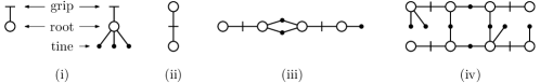
Figure 5: Fork complexes of a Heegaard splitting (ii) and of generalized Heegaard splittings (iii)–(iv). Reproduced from [26, Figure 1].

Informally, a fork complex $\boldsymbol{F}$ (representing a given generalized Heegaard splitting of a $3$-manifold $\mathcal{M}$) is obtained by taking several forks (corresponding to the compression bodies which constitute $\mathcal{M}$), and identifying grips with grips, and tines with tines (following the way the boundaries of these compression bodies are glued together). The set of grips and tines which remain unpaired is denoted by $\partial\boldsymbol{F}$ (as they correspond to surfaces which constitute the boundary $\partial\mathcal{M}$). See Figure 5 for illustrations, and [52, Section 5.1] for further details.

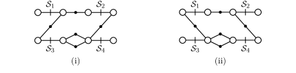
Figure 6: Fork complexes representing the generalized Heegaard splittings shown on Figure 4.

Amalgamations.

Introduced by Schultens in [54], amalgamation is a useful procedure that turns a generalized Heegaard splitting into a classical one. There are several excellent references where amalgamations are discussed in detail (cf. [3, Section 2], [19, Section 2.3], [52, Section 5.4]), therefore here we rely on a simple example to illustrate this operation.

Let $\mathcal{M}=(\mathcal{N}_{1}\cup_{\mathcal{S}_{1}}\mathcal{K}_{1})\cup_{\mathcal{R}}(\mathcal{N}_{2}\cup_{\mathcal{S}_{2}}\mathcal{K}_{2})$ be a generalized Heegaard splitting of $\mathcal{M}$, which we would like to amalgamate to form a classical Heegaard splitting $\mathcal{M}=\mathcal{N}\cup_{\mathcal{S}}\mathcal{K}$, see Figure 7. Recall that every compression body $\mathcal{C}$ can be obtained by first taking the thickened version $\partial_{-}\mathcal{C}\times[0,1]$ of its lower boundary $\partial_{-}\mathcal{C}$ and then attaching some $1$-handles to $\partial_{-}\mathcal{C}\times\{1\}$ (see steps P1 and P2 in Figure 12). In our example $\partial_{-}\mathcal{K}_{1}=\mathcal{R}=\partial_{-}\mathcal{N}_{2}$, so $\mathcal{K}_{1}$ can be built from $\mathcal{R}\times[-1,0]$ by attaching two $1$-handles $h^{(1)}_{1}$ and $h^{(1)}_{2}$ along $\mathcal{R}\times\{-1\}$. Similarly, $\mathcal{N}_{2}$ is constructed by taking $\mathcal{R}\times[0,1]$ and attaching the $1$-handles $h^{(2)}_{1}$ and $h^{(2)}_{2}$ to $\mathcal{R}\times\{1\}$.

The amalgamation process consists of two steps: 1. Collapse $\mathcal{R}\times[-1,1]$ to $\mathcal{R}\times\{0\}$, such that the attaching sites of the $1$-handles $h^{(1)}_{1}$, $h^{(1)}_{2}$, $h^{(2)}_{1}$ and $h^{(2)}_{2}$ remain pairwise disjoint. (This can be achieved by slightly deforming the attaching maps, if necessary.) 2. Set $\mathcal{N}=\mathcal{N}_{1}\cup h^{(2)}_{1}\cup h^{(2)}_{2}$ and $\mathcal{K}=\mathcal{K}_{2}\cup h^{(1)}_{1}\cup h^{(1)}_{2}$, see Figure 7(ii).

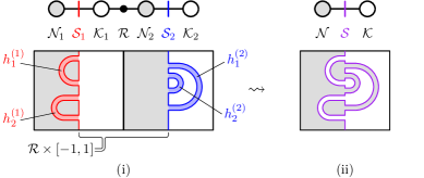
Figure 7: Amalgamating a generalized Heegaard splitting into a Heegaard splitting.

If $\mathcal{R}$ is connected, then for the genus of the amalgamated Heegaard surface $\mathcal{S}$ we have

$$g(\mathcal{S})=g(\mathcal{S}_{1})+g(\mathcal{S}_{2})-g(\mathcal{R}).$$ (5)

However, in case $\mathcal{R}$ has multiple connected components, then (5) does not hold anymore. The procedure of amalgamation nevertheless works for arbitrary generalized Heegaard splittings (cf. Remark 4), and the formula (5) can be adapted to the general setting as follows, by taking into account the Euler characteristic of the dual graph of the decomposition.

Theorem 3 (Quantitative Amalgamation; cf. Theorems 2.8 and 2.9 in [3]).

1. Any generalized Heegaard splitting $\mathcal{M}=\bigcup_{i\in I}(\mathcal{N}_{i}\cup_{\mathcal{S}_{i}}\mathcal{K}_{i})$ of a given $3$-manifold $\mathcal{M}$ can be amalgamated to a (classical) Heegaard splitting $\mathcal{M}=\mathcal{N}\cup_{\mathcal{S}}\mathcal{K}$ thereof.

2. Let $\mathscr{D}$ be the decomposition $\mathcal{M}=\bigcup_{i\in I}\mathcal{M}_{i}$ underlying the generalized Heegaard splitting above, and $\Gamma(\mathscr{D})=(I,E)$ be its dual graph with Euler characteristic $\chi(\Gamma(\mathscr{D}))$. For any $e=\{u,v\}\in E$, let $\mathcal{R}_{e}$ be the connected component of $\mathcal{M}_{u}\cap\mathcal{M}_{v}$ dual to $e$. Then the genus $g(\mathcal{S})$ of the amalgamated Heegaard surface $\mathcal{S}$ satisfies

   $$g(\mathcal{S})=\sum_{i\in I}g(\mathcal{S}_{i})-\sum_{e\in E}g(\mathcal{R}_{e})+1-\chi(\Gamma(\mathscr{D})).$$ (6)

Remark 4.

In the definition of generalized Heegaard splittings, ordering the vertices of $\Gamma(\mathscr{D})$ and choosing the Heegaard splittings of the $\mathcal{M}_{i}$ in a compatible way might seem to be an ad-hoc requirement. However, this property arises naturally, when a generalized Heegaard splitting is constructed from a sequence of handle attachments. It also ensures that a generalized Heegaard splitting can always be amalgamated into a classical one. This feature lies at the heart of many applications, including the main result of [3] according to which the problem of computing the Heegaard genus is NP-hard. We also make great use of the amalgamation procedure in Section 4 to establish Theorem 1.

2.5 Hyperbolic 3-manifolds

Hyperbolic geometry has been playing a role in the study of 3-manifolds for over a century [39], but it rose into particular prominence after Thurston formulated the geometrization conjecture [58], famously resolved by Perelman twenty years later [42, 43] (cf. [44]). Hyperbolic 3-manifolds constitute the richest family among geometric 3-manifolds, and, to this date, they remain the least understood. We refer to [38] for an introduction to this area.

A 3-manifold $\mathcal{M}$ is hyperbolic, if its interior can be obtained as a quotient of the hyperbolic 3-space $\mathbb{H}^{3}$ by a discrete group of isometries acting freely on $\mathbb{H}^{3}$. Equivalently, if the interior of $\mathcal{M}$ admits a complete Riemannian metric of constant sectional curvature $-1$. Throughout this section, $\mathcal{M}$ is assumed to be an orientable Riemannian 3-manifold. After fixing an orientation on $\mathcal{M}$, its metric tensor induces a “volume form” $\omega$. This in turn leads to the notion of volume defined via the integral

$$\operatorname{vol}(\mathcal{D})=\int_{\mathcal{D}}\omega$$

for any open set $\mathcal{D}\subseteq\mathcal{M}$. Also, any submanifold of $\mathcal{M}$ admits a Riemannian metric induced by the metric tensor of $\mathcal{M}$. Thus we may measure lengths of paths and areas of surfaces in $\mathcal{M}$ as well. We refer to [38, Section 1.2] for details.

If $\mathcal{M}$ is compact, then $\operatorname{vol}(\mathcal{M})$ is finite. The next striking result has been of paramount importance in geometric topology, as it says that “geometric properties” of finite-volume hyperbolic 3-manifolds are actually topological invariants.

Theorem 5 (Mostow Rigidity Theorem [41], cf. [2, Theorem 1.7.1], [38, Chapter 13]).

Let $\mathcal{M}$ and $\mathcal{N}$ be finite-volume hyperbolic $3$-manifolds. Every isomorphism $\pi_{1}(\mathcal{M})\rightarrow\pi_{1}(\mathcal{N})$ between the fundamental groups of $\mathcal{M}$ and $\mathcal{N}$ is induced by a unique isometry $\mathcal{M}\rightarrow\mathcal{N}$.

Corollary 6.

If two hyperbolic $3$-manifolds have different volume, then they cannot be homotopy equivalent, hence they cannot be homeomorphic.

Thick-thin decompositions.

As mentioned in the Introduction, a key ingredient in the proof of Theorem 1 is the the thick-thin decomposition theorem, a fundamentally important structural result for hyperbolic manifolds of any dimension. In order to formulate it, we need to introduce the injectivity radius of a Riemannian manifold.

Definition 7 (injectivity radius).

Let $\mathcal{M}$ be a Riemannian manifold and $x\in\mathcal{M}$. The injectivity radius of $\mathcal{M}$ at $x$, denoted $\operatorname{inj}_{x}(\mathcal{M})$, is the supremal value $r>0$ such that the metric ball of radius $r$ around $x$ is embedded in $\mathcal{M}$. The injectivity radius of $\mathcal{M}$ is defined as the infimal value of $\operatorname{inj}_{x}(\mathcal{M})$, i.e., $\operatorname{inj}(\mathcal{M})=\inf\{\operatorname{inj}_{x}(\mathcal{M}):x\in\mathcal{M}\}$.

After fixing some threshold $\varepsilon>0$, a Riemannian manifold $\mathcal{M}$ naturally decomposes into an $\varepsilon$-thick and an $\varepsilon$-thin part based on the injectivity radius of its points:

$$\mathcal{M}_{[\varepsilon,\infty)}=\{x\in\mathcal{M}:\operatorname{inj}_{x}(\mathcal{M})\geq\varepsilon/2\}\quad\text{and}\quad\mathcal{M}_{(0,\varepsilon]}=\{x\in\mathcal{M}:\operatorname{inj}_{x}(\mathcal{M})\leq\varepsilon/2\}.$$ (7)

We are now in the position to state the thick-thin decomposition theorem, according to which, for a sufficiently small constant $\varepsilon>0$ only depending on the dimension $d$, the $\varepsilon$-thin part of any orientable hyperbolic $d$-manifold has a well-understood structure.

Theorem 8 (Thick-Thin Decomposition; cf. [38, Chapter 4], [45, Section 5.3]).

There exists a universal constant $\varepsilon_{d}>0$, depending only on the dimension $d$, such that for any $\varepsilon\in(0,\varepsilon_{d}]$, the $\varepsilon$-thin part of any orientable hyperbolic $d$-manifold $\mathcal{M}$ consists of tubes around short geodesics diffeomorphic to $\mathbb{S}^{1}\times\mathbb{D}^{d-1}$, or cusps.

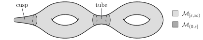
Figure 8: Thick-thin decomposition of a non-compact hyperbolic surface.

Remark 9.

We conclude with some remarks about the thick-thin decomposition.

1. In case of compact 3-manifolds, there are no cusps in the thick-thin decomposition, but only tubes. In dimension three, they are homeomorphic to solid tori. This is important, as Theorem 11 is concerned with closed (hence compact) 3-manifolds.

2. The supremum of all $\varepsilon_{d}$ for which the conclusion of Theorem 14 holds is called the $d$-dimensional Margulis constant. As of now, the precise value of $\varepsilon_{d}$ remains unknown. For $d=3$, it is known that $0.104\leq\varepsilon_{3}\leq 0.616$, cf. [45, p. 92].

3. Theorem 14 is a corollary of a more general result about discrete subgroups of Lie groups, called the Margulis Lemma, appeared in [30], cf. [38, Section 4.2] and [45, Theorem 5.22].

3 Combinatorial width parameters for 3-manifolds

Two important topological invariants we have already discussed are the Heegaard genus and the volume. Here we introduce a simple scheme that can be used to turn any non-negative graph parameter into a topological invariant for compact 3-manifolds: Given a graph parameter $p\colon\mathscr{G}\rightarrow\mathbb{N}$, defined on the set $\mathscr{G}$ of finite (multi)graphs, simply put

$$p(\mathcal{M})=\min\{p(\Gamma(\mathcal{T})):\mathcal{T}\text{\leavevmode\nobreak\ is\leavevmode\nobreak\ a\leavevmode\nobreak\ triangulation\leavevmode\nobreak\ of\leavevmode\nobreak\ }\mathcal{M}\}.$$ (8)

We call any 3-manifold invariant $p$ obtained this way a combinatorial width parameter. For reasons explained in the Introduction, in what follows, we apply this scheme on two notable graph parameters that have been playing a central role in the development of parameterized algorithms [17, 20, 21] and in structural graph theory [5, 7, 31, 34].

Treewidth and pathwidth of a graph.

Introduced by Robertson and Seymour [47, 48], the treewidth and pathwidth informally measure how tree-like or path-like a graph is. To precisely define them, we first need to talk about a tree decomposition of a graph $G=(V,E)$: it is a pair $\mathscr{T}=(\{B_{i}:i\in I\},T=(I,F))$ with bags $B_{i}\subseteq V$ and a tree $T=(I,F)$, such that

1. $\bigcup_{i\in I}B_{i}=V$,

2. for every arc $\{u,v\}\in E$, there exists $i\in I$ with $\{u,v\}\subseteq B_{i}$, and

3. for every node $v\in V$, $T_{v}=\{i\in I:v\in B_{i}\}$ spans a connected subtree of $T$.

See Figure 9 for an illustration. The width of a tree decomposition equals $\max_{i\in I}|B_{i}|-1$ and the treewidth $\operatorname{tw}(G)$ is the smallest width of any tree decomposition of $G$, cf. Figure 10.

A path decomposition of a graph $G$ is merely a tree decomposition for which the tree $T$ is required to be a path. Similarly, the pathwidth $\operatorname{pw}(G)$ of a graph $G$ is the minimum width of any path decomposition of $G$. From the definitions, $\operatorname{tw}(G)\leq\operatorname{pw}(G)$.

Figure 9: (i) A graph $G$ and a tree decomposition thereof, modeled on a tree $T$, of width 2. This tree decomposition also happens to be a path decomposition as $T$ is a path. (ii) Illustration of properties 1 and 2 from the definition of a tree decomposition: The union of all bags equals $V$, and for every arc in $E$ there is a bag containing that arc. (iii) Illustration of property 3: The bags containing a given node (in this case $c$) span a connected subtree of $T$.

Figure 10: (i) Graphs of treewidth one are precisely the trees (possibly with loops or multiarcs). (ii) A graph of treewidth two. (iii) The $k\times k$-grid (above $k=5$) has treewidth and pathwidth equal to $k$, thus planar graphs can have arbitrary large treewidth. (iv) The complete graph $K_{n}$ has treewidth $n-1$.

Treewidth and pathwidth of a 3-manifold.

Having defined the treewidth and the pathwidth of a graph, based on (8) it is immediate to extend these notions to 3-manifolds as

$$\begin{split}\operatorname{tw}(\mathcal{M})&=\min\{\operatorname{tw}(\Gamma(\mathcal{T})):\mathcal{T}\text{\leavevmode\nobreak\ is\leavevmode\nobreak\ a\leavevmode\nobreak\ triangulation\leavevmode\nobreak\ of\leavevmode\nobreak\ }\mathcal{M}\}\text{,\leavevmode\nobreak\ and}\\ \operatorname{pw}(\mathcal{M})&=\min\{\operatorname{pw}(\Gamma(\mathcal{T})):\mathcal{T}\text{\leavevmode\nobreak\ is\leavevmode\nobreak\ a\leavevmode\nobreak\ triangulation\leavevmode\nobreak\ of\leavevmode\nobreak\ }\mathcal{M}\}.\end{split}$$ (9)

As $\operatorname{tw}(G)\leq\operatorname{pw}(G)$ for any graph $G$, we also have $\operatorname{tw}(\mathcal{M})\leq\operatorname{pw}(\mathcal{M})$ for any 3-manifold $\mathcal{M}$.

Recently, the quantitative relationship between these (and related) parameters and other topological invariants has become the subject of intense research. In [26, Theorem 4] it was shown that, for any closed, irreducible, non-Haken 3-manifold $\mathcal{M}$, the treewidth $\operatorname{tw}(\mathcal{M})$ is bounded below in terms of the Heegaard genus $\mathfrak{g}\left(\mathcal{M}\right)$ by means of the following inequality:

$$\mathfrak{g}\left(\mathcal{M}\right)\leq 18(\operatorname{tw}(\mathcal{M})+1).$$ (10)

The proof of (10) relies on the theory of generalized Heegaard splittings (see [26, Section 6] for details) and, in combination with work of Agol [1], implies the existence of 3-manifolds with arbitrary large treewidth. In subsequent work [25] it was proven (based on the theory of layered triangulations [29]) that a reverse inequality holds for all closed 3-manifolds.

Theorem 10.

For every closed $3$-manifold $\mathcal{M}$ with treewidth $\operatorname{tw}(\mathcal{M})$, pathwidth $\operatorname{pw}(\mathcal{M})$, and Heegaard genus $\mathfrak{g}\left(\mathcal{M}\right)$ we have

$$\operatorname{tw}(\mathcal{M})\leq\operatorname{pw}(\mathcal{M})\leq 4\mathfrak{g}\left(\mathcal{M}\right)-2.$$ (11)

Here the first inequality follows from the definitions of pathwidth and treewidth (see above); for details about the second one, we refer to [24, Theorems 1.6 and 2.4] and [24, Chapter 5], where further refinements of these results are discussed along with related work by others.

4 The proof of Theorem 1

In this section we put together the ingredients discussed before, in order to prove that the volume of a closed hyperbolic 3-manifold provides a linear upper bound on its pathwidth.

The proof of Theorem 1 rests on Theorem 11, a folklore result according to which the Heegaard genus of a closed, orientable, hyperbolic 3-manifold can be upper-bounded in terms of its volume (see, e.g., [56, p. 336–337] or [46]).

Theorem 11.

There exists a universal constant $C^{\prime\prime}>0$ such that, for any closed, orientable, hyperbolic 3-manifold $\mathcal{M}$ with Heegaard genus $\mathfrak{g}\left(\mathcal{M}\right)$ and volume $\operatorname{vol}(\mathcal{M})$, we have

$$\mathfrak{g}\left(\mathcal{M}\right)\leq C^{\prime\prime}\cdot\operatorname{vol}(\mathcal{M}).\vspace{-\topsep}$$ (12)

Proof of Theorem 1 assuming Theorem 11.

By combining (12) with the second inequality in (11) the statement of Theorem 1 is readily deduced. ∎

We are left with proving Theorem 11. As we were unable to locate a proof of this result in the literature, below we give a proof ourselves.

Proof of Theorem 11.

First, we describe the general strategy. Given a closed, orientable, hyperbolic 3-manifold $\mathcal{M}$, we start by taking a thick-thin decomposition of $\mathcal{M}$. By a theorem that goes back to Jørgensen and Thurston, the thick part can always be triangulated using $O(\operatorname{vol}(\mathcal{M}))$ tetrahedra. Next, we show that such a triangulation of the thick part lends itself to a generalized Heegaard splitting of $\mathcal{M}$, where the sum of genera of the Heegaard surfaces is $O(\operatorname{vol}(\mathcal{M}))$. In the final step, we amalgamate this generalized Heegaard splitting into a classical Heegaard splitting of $\mathcal{M}$, and show that its genus is $O(\operatorname{vol}(\mathcal{M}))$.

We now elaborate on the details. First, we invoke the aforementioned theorem by Jørgensen–Thurston, carefully proved by Kobayashi–Rieck. To precisely state this result, let us define the (closed) $\delta$-neighborhood $\overline{N_{\delta}\vphantom{\scalebox{1.2}{$N_{\delta}$}}}\left(\mathcal{X}\right)$ of a subset $\mathcal{X}$ of a Riemannian 3-manifold $\mathcal{M}$ to be the set of those points in $\mathcal{M}$ that have distance at most $\delta$ from some point in $\mathcal{X}$.

Theorem 12 (Jørgensen–Thurston [60, §5.11], Kobayashi–Rieck [33]).

Let $\varepsilon\in(0,\varepsilon_{3}]$, where $\varepsilon_{3}$ is the Margulis constant in dimension three (cf. Remark 9/2).

1. For any $\delta>0$, there exists a constant $K>0$, depending on $\varepsilon$ and $\delta$, so that for any finite-volume hyperbolic $3$-manifold $\mathcal{M}$, the $\delta$-neighborhood $\overline{N_{\delta}\vphantom{\scalebox{1.2}{$N_{\delta}$}}}\left(\mathcal{M}_{[\varepsilon,\infty)}\right)\subset\mathcal{M}$ of the thick part $\mathcal{M}_{[\varepsilon,\infty)}$ admits a triangulation with at most $K\cdot\operatorname{vol}(\mathcal{M})$ tetrahedra.

2. Moreover, $\overline{N_{\delta}\vphantom{\scalebox{1.2}{$N_{\delta}$}}}\left(\mathcal{M}_{[\varepsilon,\infty)}\right)$ is obtained from $\mathcal{M}$ by removing open tubular neighborhoods around short geodesics, and truncating cusps [33, Proposition 1.2].

Now we fix an $\varepsilon\in(0,\varepsilon_{3}]$ and some $\delta>0$. Let $\mathcal{M}$ be a closed hyperbolic 3-manifold. In the work of Maria–Purcell [36], Theorem 12 plays a crucial role in ensuring the treewidth of $\overline{N_{\delta}\vphantom{\scalebox{1.2}{$N_{\delta}$}}}\left(\mathcal{M}_{[\varepsilon,\infty)}\right)$ to be upper-bounded by a linear function of $\operatorname{vol}(\mathcal{M})$, and that $\partial\overline{N_{\delta}\vphantom{\scalebox{1.2}{$N_{\delta}$}}}\left(\mathcal{M}_{[\varepsilon,\infty)}\right)$ can be filled with solid tori. For proving Theorem 11, we utilize Theorem 12 differently:

Proposition 13.

Let $\mathcal{Y}=\overline{N_{\delta}\vphantom{\scalebox{1.2}{$N_{\delta}$}}}\left(\mathcal{M}_{[\varepsilon,\infty)}\right)$ as defined above. The following are true.

1. For the Heegaard genus of $\mathcal{Y}$ we have $\mathfrak{g}\left(\mathcal{Y}\right)=O(\operatorname{vol}(\mathcal{M}))$.

2. $\mathcal{Y}$ has $O(\operatorname{vol}(\mathcal{M}))$ boundary components, each of which are tori.

Proof of Proposition 13.

To establish (a), first consider a triangulation $\mathcal{T}$ of $\mathcal{Y}$ with $O(\operatorname{vol}(\mathcal{M}))$ tetrahedra. Such a triangulation is guaranteed to exist by Theorem 12/1. Fix an arbitrary partition $\mathscr{P}=\{\partial_{1}\mathcal{Y},\partial_{2}\mathcal{Y}\}$ of the boundary components of $\mathcal{Y}$ (the trivial partition, i.e., $\partial_{1}\mathcal{Y}=\emptyset$, $\partial_{2}\mathcal{Y}=\partial\mathcal{Y}$, is also allowed). Follow a procedure similar to [52, Theorem 2.1.11] to obtain a Heegaard splitting of $\mathcal{Y}$ compatible with $\mathscr{P}$. (For more details, see Example 16 in Appendix B.) By construction, the genus of this splitting is $O(\operatorname{vol}(\mathcal{M}))$, hence, for the Heegaard genus of $\mathcal{Y}$, we have $\mathfrak{g}\left(\mathcal{Y}\right)=O(\operatorname{vol}(\mathcal{M}))$. For the first part of (b), observe that, by passing to a first barycentric subdivision, we may assume a tetrahedron can contribute triangles to at most one boundary component. The second part of (b) follows from Theorem 12/2. ∎

As discussed in Section 2.4, any decomposition $\mathcal{M}=\bigcup_{i\in I}\mathcal{M}_{i}$ of a 3-manifold $\mathcal{M}$ into codimension zero submanifolds with pairwise disjoint interiors gives rise to generalized Heegaard splittings of $\mathcal{M}$. Because $\mathcal{M}$ is hyperbolic, this is also true for every thick-thin decomposition of $\mathcal{M}$. So let us proceed by taking a thick-thin decomposition

$$\mathscr{D}=\left\{\mathcal{M}_{i}:i\in[m],\leavevmode\nobreak\ \textstyle\bigcup_{i=1}^{m}\mathcal{M}_{i}=\mathcal{M},\leavevmode\nobreak\ \text{and}\leavevmode\nobreak\ \operatorname{int}(\mathcal{M}_{i})\cap\operatorname{int}(\mathcal{M}_{j})=\emptyset\leavevmode\nobreak\ \text{for}\leavevmode\nobreak\ i\neq j\right\}$$ (13)

of $\mathcal{M}$, where $\mathcal{M}_{1}=\mathcal{Y}=\overline{N_{\delta}\vphantom{\scalebox{1.2}{$N_{\delta}$}}}\left(\mathcal{M}_{[\varepsilon,\infty)}\right)$ is the thick part and $\mathcal{M}_{2}\ldots,\mathcal{M}_{m}$ are the thin ones.

Note that, by Theorem 12/2, each $\mathcal{M}_{i}$ ($2\leq i\leq m$) is homeomorphic to a solid torus $\mathbb{S}^{1}\times\mathbb{D}^{2}$, and $m=O(\operatorname{vol}(\mathcal{M}))$ by Proposition 13/(b). Let us label the nodes of $\Gamma(\mathscr{D})$ via the identity map. For each $i\in[m]$, we choose a Heegaard splitting $\mathcal{M}_{i}=\mathcal{N}_{i}\cup_{\mathcal{S}_{i}}\mathcal{K}_{i}$ of minimal genus compatible with this labeling. This gives a generalized Heegaard splitting $\mathcal{M}=\bigcup_{i\in I}(\mathcal{N}_{i}\cup_{\mathcal{S}_{i}}\mathcal{K}_{i})$ of the hyperbolic 3-manifold $\mathcal{M}$. See Figure 11 for an illustration.

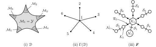
Figure 11: (i) Schematic example of a thick-thin decomposition $\mathscr{D}$ of a hyperbolic 3-manifold $\mathcal{M}$. (ii) The dual graph $\Gamma(\mathscr{D})$ of $\mathscr{D}$ with its nodes labeled via the identity map. (iii) The fork complex $\boldsymbol{F}$ of a generalized Heegaard splitting associated with $\mathscr{D}$ and the given labeling of $V(\Gamma(\mathscr{D}))$

Claim 14.

From the construction it directly follows that the generalized Heegaard splitting $\mathcal{M}=\bigcup_{i\in I}(\mathcal{N}_{i}\cup_{\mathcal{S}_{i}}\mathcal{K}_{i})$ described above has the following properties:

1. All the $\mathcal{N}_{i}$ are handlebodies. For $\mathcal{N}_{1}$ we have $g(\partial\mathcal{N}_{1})=g(\mathcal{S}_{1})=O(\operatorname{vol}(\mathcal{M}))$.

2. If $2\leq i\leq m$, then $\mathcal{N}_{i}$ is a solid torus, therefore $g(\partial\mathcal{N}_{i})=g(\mathcal{S}_{i})=1$.

3. $\mathcal{K}_{1}$ is a compression body with $\partial_{+}\mathcal{K}_{1}=\mathcal{S}_{1}$ and $\partial_{-}\mathcal{K}_{1}=\text{``disjoint union of $m$ tori.''}$

4. If $2\leq i\leq m$, then $\mathcal{K}_{i}$ is a trivial compression body homeomorphic to $\mathbb{T}^{2}\times[0,1]$. For its boundary components we have $\partial_{+}\mathcal{K}_{i}=\mathcal{S}_{i}$ and $\partial_{-}\mathcal{K}_{i}=\mathcal{R}_{i}=\mathcal{M}_{i}\cap\mathcal{M}_{1}$.

5. For the sum of the genera of the surfaces $\mathcal{S}_{i}$ we have $\sum_{i=1}^{m}g(\mathcal{S}_{i})=O(\operatorname{vol}(\mathcal{M}))$. $\vartriangleleft$

By Theorem 3, we may amalgamate this to a classical Heegaard splitting $\mathcal{M}=\mathcal{N}\cup_{\mathcal{S}}\mathcal{K}$. Finally, by combining the data from Claim 14 with the formula (6) in Theorem 3, we get

$$g(\mathcal{S}) =\sum_{i\in I}g(\mathcal{S}_{i})-\sum_{e\in E}g(\mathcal{R}_{e})+1-\chi(\Gamma(\mathscr{D}))$$ (14)

$$=g(\mathcal{S}_{1})+\sum_{i=2}^{m}\left(g(\mathcal{S}_{i})-g(\mathcal{R}_{i})\right)+1-\chi(\Gamma(\mathscr{D}))$$ (15)

$$=O(\operatorname{vol}(\mathcal{M}))+\sum_{i=2}^{m}\left(1-1\right)+1-1=O(\operatorname{vol}(\mathcal{M})).$$ (16)

This concludes the proof of Theorem 11. ∎

5 Discussion

Pathwidth vs. treewidth vs. volume.

The inequalities (1) and (2) respectively provide information about the quantitative relationship between the treewidth and the volume, and the pathwidth and the volume of hyperbolic 3-manifolds. It is natural to study the sharpness of these inequalities both in absolute terms and also relative to each other.

In [36, Section 6] Maria and Purcell show that, by performing appropriate Dehn fillings on hyperbolic $2$-bridge knot exteriors, one can obtain an infinite family of closed hyperbolic 3-manifolds with bounded treewidth, but unbounded volume. The bound on the treewidth is established through a construction of small-treewidth triangulations of these manifolds, based on the work of Sakuma–Weeks [49] on triangulating 2-bridge knot exteriors. It is not difficult to see that these triangulations have bounded pathwidth, too.

Regarding the comparison of (1) and (2), recall that, from the definitions of pathwidth and treewidth (Section 3) if follows that $\operatorname{tw}(\mathcal{M})\leq\operatorname{pw}(\mathcal{M})$ for every 3-manifold $\mathcal{M}$. However, while there are examples for which both of these quantities are small [25] or arbitrary large [26], we do not know whether their difference can be arbitrary large. Thus we ask:

Question 15.

Can the difference $\operatorname{pw}(\mathcal{M})-\operatorname{tw}(\mathcal{M})$ be arbitrary large?

Note that, in case of graphs, trees can have arbitrary large pathwidth, e.g., the complete binary tree $T_{h}$ of height $h$ satisfies $\operatorname{pw}(T_{h})=\lceil h/2\rceil$, cf. [6, Theorem 67] or [57, Lemma 2.8].

Algorithmic aspects of small pathwidth.

In the Introduction it was mentioned that input triangulations with small-pathwidth dual graphs can speed up algorithms that are fixed-parameter tractable (FPT) in the treewidth. Here we briefly elaborate on this.

A typical FPT-algorithm $\mathscr{A}$ exploits the small treewidth of the dual graph of its input triangulation by using a data structure called a nice tree decomposition. This is a particular kind of tree decomposition, whose bags can be grouped into three different types: forget, introduce, and join bags. A triangulation $\mathcal{T}$ with $n$ tetrahedra and $\operatorname{tw}(\Gamma(\mathcal{T}))=k$ always admits a nice tree decomposition with at most $4n$ bags of width $k$, see [32, Section 13.1].

Upon taking such a triangulation $\mathcal{T}$ as input, the algorithm $\mathscr{A}$ would first construct a tree decomposition $\mathscr{T}$ of $\Gamma(\mathcal{T})$ of small width, turn $\mathscr{T}$ into a nice tree decomposition $\mathscr{T}_{\mathrm{nice}}$ (which is still of small width, as noted above), then parse $\mathscr{T}_{\mathrm{nice}}$ and perform its specific computation at each bag thereof. Depending on the problem to be solved, processing a join bag can be orders of magnitudes slower than processing an introduce or forget bag (we refer to [26, Appendix C] for more details, and to [13, Section 4(d)] for a real-life example).

Now, if the decomposition $\mathscr{T}$ happens to be a path decomposition (i.e., a tree decomposition where the underlying tree is a path), then the procedure for constructing $\mathscr{T}_{\mathrm{nice}}$ results in a nice tree decomposition without join bags. Therefore, if the pathwidth $\operatorname{pw}(\Gamma(\mathcal{T}))$ is not “much” larger than the treewidth $\operatorname{tw}(\Gamma(\mathcal{T}))$, constructing a path decomposition (instead of an arbitrary tree decomposition) in the first step can potentially be very beneficial for the overall running time of $\mathscr{A}$, as the algorithm does not have to deal with join bags at all.

Topological parameters for FPT-algorithms.

Algorithms that are FPT in the treewidth have been very successful in 3-dimensional topology. They all come with a caveat though: their fast execution presumes an input triangulation whose dual graph has small treewidth. However, in case the triangulation at hand has high treewidth, finding another triangulation of the same 3-manifold that has smaller treewidth might be very difficult.

To address this challenge, recently there has been a growing interest in researching algorithms that are FPT in topological parameters (e.g., the first Betti number [37]), that do not depend on the particular input triangulation, but only on the underlying 3-manifold.

Together with [36], our work reinforces the potential of the volume of becoming a useful topological parameter for FPT-algorithms in the realm of hyperbolic 3-manifolds.

Appendix A The primal and dual construction of compression bodies

Appendix B Heegaard splittings of 3-manifolds with boundary

Example 16 (Heegaard splittings from triangulations, II – based on [52, Theorem 2.1.11]).

Let $\mathcal{T}$ be a triangulation of $\mathcal{M}$ with partition $\partial_{1}\mathcal{M}\cup\partial_{2}\mathcal{M}$ of its boundary components. Suppose that no simplex in $\mathcal{T}$ is incident to more than one component of $\partial\mathcal{M}$. Take the first barycentric subdivision $\operatorname{sd}_{1}(\mathcal{T})$ of $\mathcal{T}$. Recall that $\mathcal{T}^{(1)}$ and $\Gamma(\mathcal{T})$ denote the 1-skeleton and the dual graph of $\mathcal{T}$. Their first barycentric subdivisons $\mathcal{T}^{(1)}_{\operatorname{sd}}$ and $\Gamma(\mathcal{T})_{\operatorname{sd}}$ are both naturally contained in $\operatorname{sd}_{1}(\mathcal{T})$. Consider the subcomplex $N(\partial_{2}\mathcal{M})\subset\operatorname{sd}_{1}(\mathcal{T})$ consisting of all simplices incident to $\partial_{2}\mathcal{M}$. We define two further subcomplexes of $\operatorname{sd}_{1}(\mathcal{T})$, namely

• $\Gamma_{1}=\partial_{1}\mathcal{M}\cup\{\text{vertices and edges of $\mathcal{T}^{(1)}_{\operatorname{sd}}$ {\em not} incident to $\partial_{2}\mathcal{M}$}\}$, and

• $\Gamma_{2}=N(\partial_{2}\mathcal{M})\cup\Gamma(\mathcal{T})_{\operatorname{sd}}.$

Now pass to the second barycentric subdivision $\operatorname{sd}_{2}(\mathcal{T})$ and let $(\Gamma_{i})_{\operatorname{sd}}$ denote the image of $\Gamma_{i}$ under this operation ($i=1,2$). Let $\eta(\Gamma_{i})$ be the “thickening” of $\Gamma_{i}$, i.e., the subcomplex of $\operatorname{sd}_{2}(\mathcal{T})$ formed by all simplices incident to $(\Gamma_{i})_{\operatorname{sd}}$. One can readily verify that $\eta(\Gamma_{1})$ and $\eta(\Gamma_{2})$ are compression bodies whose union is $\mathcal{M}$, their upper boundaries satisfy $\partial_{+}\eta(\Gamma_{1})=\partial_{+}\eta(\Gamma_{2})=\eta(\Gamma_{1})\cap\eta(\Gamma_{2})$, and for their lower boundaries $\partial_{-}\eta(\Gamma_{1})=\partial_{1}\mathcal{M}$ and $\partial_{-}\eta(\Gamma_{2})=\partial_{2}\mathcal{M}$. Hence $\eta(\Gamma_{1})$ and $\eta(\Gamma_{2})$ form a Heegaard splitting of $\mathcal{M}$ compatible with the given partition of its boundary components. See Figure 13 for an illustration via “quadrangulations.”

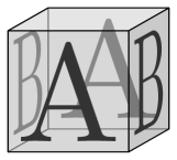
(i) $\mathcal{M}=\mathbb{T}^{2}\times[0,1]$ lorem ipsum dolor sit amet

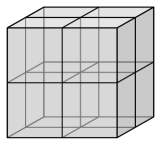
(ii) A quadrangulation $\mathcal{Q}$ of $\mathcal{M}$ with eight cubes

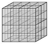
(iii) The first barycentric subdivision $\operatorname{sd}_{1}(\mathcal{Q})$ of $\mathcal{Q}$

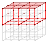
(iv) ${\color[rgb]{0.72,0,0}\boldsymbol{\Gamma_{1}}}$

${\color[rgb]{0.72,0,0}\boldsymbol{\Gamma_{1}}}=\partial_{1}\mathcal{M}\cup\{$vertices & edges of $\mathcal{T}^{(1)}_{\operatorname{sd}}$ avoiding $N(\partial_{2}\mathcal{M})\}$

${\color[rgb]{0,0,1}\boldsymbol{\Gamma_{2}}}=N(\partial_{2}\mathcal{M})\cup\Gamma(\mathcal{T})_{\operatorname{sd}}$

(v) ${\color[rgb]{0,0,1}\boldsymbol{\Gamma_{2}}}$

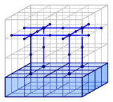
(v) ${\color[rgb]{0,0,1}\boldsymbol{\Gamma_{2}}}$

Figure 13: Building a Heegaard splitting of the thickened torus $\mathbb{T}^{2}\times[0,1]$ from a quadrangulation.

References

- [1] I. Agol. Small 3-manifolds of large genus. Geom. Dedicata, 102:53–64, 2003. doi:10.1023/B:GEOM.0000006584.85248.c5, MR:2026837, Zbl:1039.57008.
- [2] M. Aschenbrenner, S. Friedl, and H. Wilton. 3-Manifold Groups, volume 20 of EMS Ser. Lect. Math. Eur. Math. Soc. (EMS), Zürich, 2015. doi:10.4171/154, MR:3444187, Zbl:1326.57001.
- [3] D. Bachman, R. Derby-Talbot, and E. Sedgwick. Computing Heegaard genus is NP-hard. In A Journey Through Discrete Mathematics: A Tribute to Jiří Matoušek, pages 59–87. Springer, Cham, 2017. doi:10.1007/978-3-319-44479-6, MR:3726594, Zbl:1388.57020.
- [4] R. H. Bing. An alternative proof that -manifolds can be triangulated. Ann. Math. (2), 69:37–65, 1959. doi:10.2307/1970092, MR:0100841, Zbl:0106.16604.
- [5] H. L. Bodlaender. A tourist guide through treewidth. Acta Cybern., 11(1-2):1–21, 1993. urn:nbn:nl:ui:10-1874-2301. MR:1268488, Zbl:0804.68101.
- [6] H. L. Bodlaender. A partial k-arboretum of graphs with bounded treewidth. Theor. Comput. Sci., 209(1–2):1–45, 1998. doi:10.1016/S0304-3975(97)00228-4, MR:1647486, Zbl:0912.68148.
- [7] H. L. Bodlaender. Discovering treewidth. In Proc. 31st Conf. Curr. Trends Theory Pract. Comput. Sci. (SOFSEM 2005), pages 1–16, 2005. doi:10.1007/978-3-540-30577-4_1, Zbl:1117.68451.
- [8] B. A. Burton. Computational topology with Regina: algorithms, heuristics and implementations. In Geometry and Topology Down Under, volume 597 of Contemp. Math., pages 195–224. Amer. Math. Soc., Providence, RI, 2013. doi:10.1090/conm/597/11877, MR:3186674, Zbl:1279.57004.
- [9] B. A. Burton. A new approach to crushing 3-manifold triangulations. Discrete Comput. Geom., 52(1):116–139, 2014. doi:10.1007/s00454-014-9572-y, MR:3231034, Zbl:1317.57012.
- [10] B. A. Burton. The HOMFLY-PT polynomial is fixed-parameter tractable. In 34th Int. Symp. Comput. Geom. (SoCG 2018), volume 99 of LIPIcs. Leibniz Int. Proc. Inform., pages 18:1–18:14. Schloss Dagstuhl–Leibniz-Zent. Inf., 2018. doi:10.4230/LIPIcs.SoCG.2018.18, MR:3824262.
- [11] B. A. Burton, R. Budney, W. Pettersson, et al. Regina: Software for low-dimensional topology, 1999–2019. Version 5.1. URL: https://regina-normal.github.io.
- [12] B. A. Burton and R. G. Downey. Courcelle’s theorem for triangulations. J. Comb. Theory, Ser. A, 146:264–294, 2017. doi:10.1016/j.jcta.2016.10.001, MR:3574232, Zbl:1353.05122.
- [13] B. A. Burton, T. Lewiner, J. Paixão, and J. Spreer. Parameterized complexity of discrete Morse theory. ACM Trans. Math. Softw., 42(1):6:1–6:24, 2016. doi:10.1145/2738034, MR:3472422, Zbl:1347.68165.
- [14] B. A. Burton, C. Maria, and J. Spreer. Algorithms and complexity for Turaev–Viro invariants. J. Appl. Comput. Topol., 2(1–2):33–53, 2018. doi:10.1007/s41468-018-0016-2, MR:3873178, Zbl:07089248.
- [15] B. A. Burton and W. Pettersson. Fixed parameter tractable algorithms in combinatorial topology. In Proc. 20th Int. Conf. Comput. Comb. (COCOON 2014), pages 300–311, 2014. doi:10.1007/978-3-319-08783-2_26, MR:3247596, Zbl:1423.68205.
- [16] B. A. Burton and J. Spreer. The complexity of detecting taut angle structures on triangulations. In Proc. 24th Annu. ACM-SIAM Symp. Discrete Algorithms (SODA 2013), pages 168–183, 2013. doi:10.1137/1.9781611973105.13, MR:3185388, Zbl:1421.68161.
- [17] M. Cygan, F. V. Fomin, Ł. Kowalik, D. Lokshtanov, D. Marx, M. Pilipczuk, M. Pilipczuk, and S. Saurabh. Parameterized Algorithms. Springer, Cham, 2015. doi:10.1007/978-3-319-21275-3, MR:3380745, Zbl:1334.90001.
- [18] A. de Mesmay, J. Purcell, S. Schleimer, and E. Sedgwick. On the tree-width of knot diagrams. J. Comput. Geom., 10(1):164–180, 2019. doi:10.20382/jocg.v10i1a6, MR:3957223, Zbl:1432.57017.
- [19] R. Derby-Talbot. Stabilization, amalgamation and curves of intersection of Heegaard splittings. Algebr. Geom. Topol., 9(2):811–832, 2009. doi:10.2140/agt.2009.9.811, MR:2505126, Zbl:1176.57021.
- [20] R. G. Downey and M. R. Fellows. Parameterized Complexity. Monogr. Comput. Sci. Springer-Verlag New York, 1999. doi:10.1007/978-1-4612-0515-9, MR:1656112, Zbl:0914.68076.
- [21] R. G. Downey and M. R. Fellows. Fundamentals of Parameterized Complexity. Texts Comput. Sci. Springer, London, 2013. doi:10.1007/978-1-4471-5559-1, MR:3154461, Zbl:1358.68006.
- [22] P. Heegaard. Sur l’”Analysis situs”. Bull. Soc. Math. France, 44:161–242, 1916. doi:10.24033/bsmf.968, MR:1504754.
- [23] J. Hempel. 3-Manifolds. AMS Chelsea Publ., Providence, RI, 2004. Reprint of the 1976 original. doi:10.1090/chel/349, MR:2098385, Zbl:1058.57001.
- [24] K. Huszár. Combinatorial width parameters for 3-dimensonal manifolds. PhD thesis, IST Austria, June 2020. doi:10.15479/AT:ISTA:8032.
- [25] K. Huszár and J. Spreer. 3-Manifold triangulations with small treewidth. In 35th Int. Symp. Comput. Geom. (SoCG 2019), volume 129 of LIPIcs. Leibniz Int. Proc. Inf., pages 44:1–44:20. Schloss Dagstuhl–Leibniz-Zent. Inf., 2019. doi:10.4230/LIPIcs.SoCG.2019.44, MR:3968630.
- [26] K. Huszár, J. Spreer, and U. Wagner. On the treewidth of triangulated 3-manifolds. J. Comput. Geom., 10(2):70–98, 2019. doi:10.20382/jogc.v10i2a5, MR:4039886, Zbl:07150581.
- [27] W. Jaco. Lectures on Three-Manifold Topology, volume 43 of CBMS Reg. Conf. Ser. Math. Amer. Math. Soc., Providence, R.I., 1980. doi:10.1090/cbms/043, MR:565450, Zbl:0433.57001.
- [28] W. Jaco and J. H. Rubinstein. -efficient triangulations of 3-manifolds. J. Differential Geom., 65(1):61–168, 2003. doi:10.4310/jdg/1090503053, MR:2057531, Zbl:1068.57023.
- [29] W. Jaco and J. H. Rubinstein. Layered-triangulations of 3-manifolds, 2006. 97 pages, 32 figures. arXiv:math/0603601.
- [30] D. A. Každan and G. A. Margulis. A proof of Selberg’s hypothesis. Math. USSR–Sbornik, 4(1):147–152, 1968. Translation from Mat. Sb. (N.S.), 75(117):163–168, 1968. Translated by: Z. Skalsky. doi:10.1070/SM1968v004n01ABEH002782, MR:0223487, Zbl:0241.22024.
- [31] K. Kawarabayashi and B. Mohar. Some recent progress and applications in graph minor theory. Graphs Combin., 23(1):1–46, 2007. doi:10.1007/s00373-006-0684-x, MR:2292102, Zbl:1114.05096.
- [32] T. Kloks. Treewidth: Computations and Approximations, volume 842 of Lect. Notes Comput. Sci. Springer, 1994. doi:10.1007/BFb0045375, MR:1312164, Zbl:0825.68144.
- [33] T. Kobayashi and Y. Rieck. A linear bound on the tetrahedral number of manifolds of bounded volume (after Jørgensen and Thurston). In Topology and Geometry in Dimension Three, volume 560 of Contemp. Math., pages 27–42. Amer. Math. Soc., Providence, RI, 2011. doi:10.1090/conm/560/11089, MR:2866921, Zbl:1335.57028.
- [34] L. Lovász. Graph minor theory. Bull. Amer. Math. Soc. (N.S.), 43(1):75–86, 2006. doi:10.1090/S0273-0979-05-01088-8, MR:2188176, Zbl:1082.05082.
- [35] C. Maria. Parameterized complexity of quantum invariants, 2019. arXiv:1910.00477.
- [36] C. Maria and J. Purcell. Treewidth, crushing and hyperbolic volume. Algebr. Geom. Topol., 19(5):2625–2652, 2019. doi:10.2140/agt.2019.19.2625, MR:4023324, Zbl:07142614.
- [37] C. Maria and J. Spreer. A polynomial-time algorithm to compute Turaev–Viro invariants of 3-manifolds with bounded first Betti number. Found. Comput. Math., pages 1–22, 2019. Online: 11.11.2019. doi:10.1007/s10208-019-09438-8.
- [38] B. Martelli. An Introduction to Geometric Topology. CreateSpace, 2016. URL: http://people.dm.unipi.it/martelli/geometric_topology.html, arXiv:1610.02592.
- [39] C. T. McMullen. The evolution of geometric structures on 3-manifolds. Bull. Amer. Math. Soc. (N.S.), 48(2):259–274, 2011. doi:10.1090/S0273-0979-2011-01329-5, MR:2774092, Zbl:1214.57017.
- [40] E. E. Moise. Affine structures in -manifolds. V. The triangulation theorem and Hauptvermutung. Ann. Math. (2), 56:96–114, 1952. doi:10.2307/1969769, MR:0048805, Zbl:0048.17102.
- [41] G. D. Mostow. Quasi-conformal mappings in -space and the rigidity of hyperbolic space forms. Publ. Math. IHÉS, 34:53–104, 1968. URL: http://www.numdam.org/item?id=PMIHES_1968__34__53_0, MR:236383, Zbl:0189.09402.
- [42] G. Perelman. The entropy formula for the Ricci flow and its geometric applications, 2002. 39 pages. arXiv:math/0211159.
- [43] G. Perelman. Ricci flow with surgery on three-manifolds, 2003. 22 pages. arXiv:math/0303109.
- [44] J. Porti. Geometrization of three manifolds and Perelman’s proof. Rev. R. Acad. Cienc. Exactas Fís. Nat. Ser. A Math. RACSAM, 102(1):101–125, 2008. doi:10.1007/BF03191814, MR:2416241, Zbl:1170.57016.
- [45] J. S. Purcell. Hyperbolic Knot Theory (preprint). February 2020. URL: http://users.monash.edu/~jpurcell/book/HypKnotTheory.pdf, arXiv:2002.12652.
- [46] J. S. Purcell and A. Zupan. Independence of volume and genus bridge numbers. Proc. Amer. Math. Soc., 145(4):1805–1818, 2017. doi:10.1090/proc/13327, MR:3601570, Zbl:1364.57009.
- [47] N. Robertson and P. D. Seymour. Graph minors. I. Excluding a forest. J. Comb. Theory, Ser. B, 35(1):39–61, 1983. doi:10.1016/0095-8956(83)90079-5, MR:723569, Zbl:0521.05062.
- [48] N. Robertson and P. D. Seymour. Graph minors. II. Algorithmic aspects of tree-width. J. Algorithms, 7(3):309–322, 1986. doi:10.1016/0196-6774(86)90023-4, MR:855559, Zbl:0611.05017.
- [49] M. Sakuma and J. Weeks. Examples of canonical decompositions of hyperbolic link complements. Japan. J. Math. (N.S.), 21(2):393–439, 1995. doi:10.4099/math1924.21.393, MR:1364387, Zbl:0858.57021.
- [50] N. Saveliev. Lectures on the Topology of 3-Manifolds: An Introduction to the Casson Invariant. De Gruyter Textbook. Walter de Gruyter & Co., Berlin, 2nd edition, 2012. doi:10.1515/9783110250367, MR:2893651, Zbl:1246.57003.
- [51] M. Scharlemann. Heegaard splittings of compact 3-manifolds. In Handbook of Geometric Topology, pages 921–953. North-Holland, Amsterdam, 2001. doi:10.1016/B978-044482432-5/50019-6, MR:1886684, Zbl:0985.57005.
- [52] M. Scharlemann, J. Schultens, and T. Saito. Lecture Notes on Generalized Heegaard Splittings. World Scientific Publishing Co. Pte. Ltd., Hackensack, NJ, 2016. doi:10.1142/10019, MR:3585907, Zbl:1356.57004.
- [53] M. Scharlemann and A. Thompson. Thin position for -manifolds. In Geometric topology (Haifa, 1992), volume 164 of Contemp. Math., pages 231–238. Amer. Math. Soc., Providence, RI, 1994. doi:10.1090/conm/164/01596, MR:1282766, Zbl:0818.57013.
- [54] J. Schultens. The classification of Heegaard splittings for (compact orientable surface). Proc. London Math. Soc. (3), 67(2):425–448, 1993. doi:10.1112/plms/s3-67.2.425, MR:1226608, Zbl:0789.57012.
- [55] J. Schultens. Introduction to 3-Manifolds, volume 151 of Grad. Stud. Math. Amer. Math. Soc., Providence, RI, 2014. doi:10.1090/gsm/151, MR:3203728, Zbl:1295.57001.
- [56] P. B. Shalen. Hyperbolic volume, Heegaard genus and ranks of groups. In Workshop on Heegaard Splittings, volume 12 of Geom. Topol. Monogr., pages 335–349. Geom. Topol. Publ., Coventry, 2007. doi:10.2140/gtm.2007.12.335, MR:2408254, Zbl:1140.57009.
- [57] A. Takahashi, S. Ueno, and Y. Kajitani. Minimal acyclic forbidden minors for the family of graphs with bounded path-width. Discrete Math., 127(1–3):293–304, 1994. doi:10.1016/0012-365X(94)90092-2, MR:1273610, Zbl:0795.05123.
- [58] W. P. Thurston. Three-dimensional manifolds, Kleinian groups and hyperbolic geometry. Bull. Amer. Math. Soc. (N.S.), 6(3):357–381, 1982. doi:10.1090/S0273-0979-1982-15003-0, MR:648524, Zbl:0496.57005.
- [59] W. P. Thurston. Three-Dimensional Geometry and Topology. Vol. 1, volume 35 of Princeton Math. Ser. Princeton Univ. Press, Princeton, NJ, 1997. Edited by S. Levy. doi:10.1515/9781400865321, MR:1435975, Zbl:0873.57001.
- [60] W. P. Thurston. The geometry and topology of three-manifolds. Electronic version 1.1, March, 2002. URL: http://library.msri.org/books/gt3m.