Learning Security Classifiers with
Verified Global Robustness Properties

Abstract.

Many recent works have proposed methods to train classifiers with local robustness properties, which can provably eliminate classes of evasion attacks for most inputs, but not all inputs. Since data distribution shift is very common in security applications, e.g., often observed for malware detection, local robustness cannot guarantee that the property holds for unseen inputs at the time of deploying the classifier. Therefore, it is more desirable to enforce global robustness properties that hold for all inputs, which is strictly stronger than local robustness.

In this paper, we present a framework and tools for training classifiers that satisfy global robustness properties. We define new notions of global robustness that are more suitable for security classifiers. We design a novel booster-fixer training framework to enforce global robustness properties. We structure our classifier as an ensemble of logic rules and design a new verifier to verify the properties. In our training algorithm, the booster increases the classifier’s capacity, and the fixer enforces verified global robustness properties following counterexample guided inductive synthesis.

We show that we can train classifiers to satisfy different global robustness properties for three security datasets, and even multiple properties at the same time, with modest impact on the classifier’s performance. For example, we train a Twitter spam account classifier to satisfy five global robustness properties, with $5.4\%$ decrease in true positive rate, and $0.1\%$ increase in false positive rate, compared to a baseline XGBoost model that doesn’t satisfy any property.

1. Introduction

Machine learning classifiers can achieve high accuracy to detect malware, spam, phishing, online fraud, etc., but they are brittle against evasion attacks. For example, to detect whether a Twitter account is spamming malicious URLs, many research works have proposed to use content-based features, such as the number of tweets containing URLs from that account (Lee et al., 2010; Lee and Kim, 2013; Ma et al., 2009; Thomas et al., 2011). These features are useful at achieving high accuracy, but attackers can easily modify their behavior to evade the classifier.

In this paper, we develop a framework and tools for addressing this problem. First, the defenders identify a property $\varphi$ that the classifier should satisfy; typically, $\varphi$ identifies a class of evasion strategies that might be available to an adversary, and specifies a requirement on their effect on the classifier (e.g., that they won’t change the classifier’s output too much). Next, the defenders train a classifier $\mathcal{F}$ that satisfies $\varphi$. We identify several properties $\varphi$ that capture different notions of classifier robustness. Then, we design an algorithm for the classifier design problem:

Given a property $\varphi$ and a training set $\mathcal{D}$, train a classifier $\mathcal{F}$ that satisfies $\varphi$.

Our algorithm trains a verifiably robust classifier: we can formally verify that $\mathcal{F}$ satisfies $\varphi$.

Existing works focus on training and verifying local robustness properties of classifiers. Typically, they verify the following local robustness property: define $\varphi(x)$ to be the assertion that for all $x^{\prime}$, if $\lVert x^{\prime}-x\rVert_{p}\leq\epsilon$, then $\mathcal{F}(x^{\prime})$ is classified the same as $\mathcal{F}(x)$. The past works provide a way to verify whether $\varphi(x)$ holds, for a fixed $x$, and then devise ways to train a classifier $\mathcal{F}$ so that $\varphi(x)$ holds for most $x$, but not all $x$ (local robustness). So far, the most promising defenses against adversarial examples all take this form, including adversarial training (Madry et al., 2018), certifiable training (Dvijotham et al., 2018a; Mirman et al., 2018; Wong and Kolter, 2018; Wang et al., 2018a), and randomized smoothing techniques (Li et al., 2018; Lecuyer et al., 2019; Cohen et al., 2019b). To evaluate the local robustness of a trained model, we can measure the percentage of data points $x$ in the test set that satisfy $\varphi(x)$ (Lomuscio and Maganti, 2017; Katz et al., 2017; Huang et al., 2017; Ehlers, 2017; Fischetti and Jo, 2017; Dutta et al., 2018; Raghunathan et al., 2018a; Weng et al., 2018a; Gehr et al., 2018; Wang et al., 2018c; Singh et al., 2019c, b; Wang et al., 2018b; Wong and Kolter, 2018; Raghunathan et al., 2018b; Tjeng et al., 2017; Dvijotham et al., 2018b). This measurement is useful if at the time of deploying the classifier, the real-world data follow the same distribution as the measured test set. Unfortunately, data distribution shift is very common in security applications (e.g., malware detection (Pendlebury et al., 2019; Allix et al., 2015; Miller et al., 2016)), so local robustness cannot guarantee that the robustness property holds for most inputs at deployment time. In fact, in some cases, the adversary may be able to adapt their behavior by choosing novel samples $x$ that don’t follow the test distribution and such that $\varphi(x)$ doesn’t hold.

In this paper, we address these challenges by showing how to train classifiers that satisfy verified global robustness properties. We define a global robustness property as a universally quantified statement over one or more inputs to the classifier, and its corresponding outputs: e.g., $\forall x.\varphi(x)$ or $\forall x,x^{\prime}.\varphi(x,x^{\prime})$. Since global robustness holds for all inputs, it is strictly stronger than local robustness, and it ensures robustness even under distribution shift. Then, we identify a number of robustness properties that may be useful in security applications, and we develop a general technique to achieve the properties. Our technique can handle a large class of properties, formally defined in Section 5.2.1. The vast majority of past work has focused on $\ell_{p}$ robustness, perhaps motivated by computer vision; however, in security settings, such as detecting malware, online fraud, or other attacks, other notions of robustness may be more appropriate.

There are many challenges in training classifiers with global robustness properties. First, it is hard to maintain good test accuracy since the definition of global robustness is much stronger than local robustness. To the best of our knowledge, among global robustness properties, only two properties have been previously achieved. One of them is monotonicity  (Incer et al., 2018; Wehenkel and Louppe, 2019); and the other is a concurrent work that has proposed $\ell_{p}$-norm robustness with the option to abstain on non-robust inputs (Leino et al., 2021). For example, researchers have trained a monotonic malware classifier to defend against evasion attacks that add content to a malware (Incer et al., 2018). Monotonicity is useful: it limits the attacker to more expensive evasion operations that may remove malicious functionality from the malware, if they want to evade the classifier. However, monotonicity is not general enough to capture some types of evasion. Second, it is challenging to train classifiers with guarantees of global robustness. Several training techniques sacrifice global robustness in their algorithms. For example, DL2 (Fischer et al., 2019) proposed several global robustness properties, but their training technique only achieves local robustness and cannot learn classifiers with global properties, because they rely on adversarial training. ART (Lin et al., 2020) presents an abstraction refinement method to train neural networks with global robustness properties. In principle ART can guarantee global robustness if the correctness loss reaches zero, however in their experiments the loss never reached zero.

To overcome these challenges, we design a novel booster-fixer training framework that enforces global robustness. Our classifier is structured as an ensemble of logic rules—a new architecture that is more expressive than trees given the same number of atoms and clauses (formally defined in Section 4.1)—and we show how to verify global robustness properties and then how to train them, for these ensembles. Intuitively, our algorithm trains a candidate classifier with good accuracy (but not necessarily any robustness), and then we fix the classifier to satisfy global robustness by iteratively finding counterexamples and repairing them using the Counterexample Guided Inductive Synthesis (CEGIS) paradigm (Solar-Lezama et al., 2006). Past works for training monotonic classifiers all use specialized techniques that do not generalize to other properties (Wehenkel and Louppe, 2019; Incer et al., 2018; Archer and Wang, 1993; Daniels and Velikova, 2010; Kay and Ungar, 2000; Ben-David, 1995; Duivesteijn and Feelders, 2008; Feelders, 2010; Gupta et al., 2016). In contrast, our technique is fully general and can handle a large class of global robustness properties (formally defined in Section 5.2.1); we even show that we can enforce multiple properties at the same time (Section 3.2, Section 6.3.3).

We evaluate our approach on three security datasets: cryptojacking (Kharraz et al., 2019), Twitter spam accounts (Lee et al., 2011), and Twitter spam URLs (Kwon et al., 2017). Using security domain knowledge and results from measurement studies, we specify desirable global robustness properties for each classification task. We show that we can train all properties individually, and we can even enforce multiple properties at the same time, with a modest impact on the classifier’s performance. For example, we train a classifier to detect Twitter spam accounts while satisfying five global robustness properties; the true positive rate decreases by $5.4\%$ and the false positive rate increases by $0.1\%$, compared to a baseline XGBoost model that doesn’t satisfy any robustness property.

Since no existing work can train classifiers with any global robustness property other than monotonicity, we compare our approach against two types of baseline models: 1) monotonic classifiers, and 2) models trained with local versions of our proposed properties. For the monotonicity property, our results show that our method can achieve comparable or better model performance than prior methods that were specialized for monotonicity. We also verify that we can enforce each global robustness property we consider, which no prior method achieves for any of the other properties.

Our contributions are summarized as follows.

• We define new global robustness properties that are relevant for security applications.

• We design and implement a general booster-fixer training procedure to train classifiers with verified global robustness properties.

• We propose a new type of model, logic ensemble, that is well-suited to booster-fixer training. We show how to verify properties of such a model.

• We are the first to train multiple global robustness properties. We demonstrate that we can enforce these properties while maintaining high test accuracy for detecting cryptojacking websites, Twitter spam accounts, and Twitter spam URLs. Our code is available at https://github.com/surrealyz/verified-global-properties.

2. Example

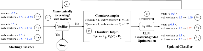
Figure 1. One CEGIS iteration of our training algorithm, illustrated on a simple example. Here we train a classifier to detect cryptojacking, while enforcing a monotonicity property.

In this section, we present an illustrative example to show how our training algorithm works. Within our booster-fixer framework, the fixer follows the Counterexample Guided Inductive Synthesis (CEGIS) paradigm. The key step in each CEGIS iteration is to start from a classifier without the global robustness property, use a verifier to find counterexamples that violate the property, and train the classifier for one epoch guided by the counterexample. This process is repeated until the classifier satisfies the property. Here, we show how to train one CEGIS iteration for a classifier to detect cryptojacking web pages. For simplicity, we demonstrate classification using only two features.

2.1. Monotonicity for Cryptojacking Classifier

We use two features to detect cryptojacking: whether the website uses WebAssembly (wasm), and the number of web workers used by the website (Kharraz et al., 2019). Cryptojacking websites need the high performance provided by WebAssembly and often use multiple web worker threads to mine cryptocurrency concurrently. We enforce a monotonicity property for the web workers feature: the more web workers a website uses, the more suspicious it should be rated by the classifier, with all else held equal.

Figure 1 shows a single CEGIS iteration that starts from a classifier that violates the property, uses a counterexample to guide the training, and arrives at an updated classifier that satisfies the property. The classifier is structured as an ensemble of logic rules. For example, “$\texttt{wasm}<0.5\land\texttt{web workers}<1.5\rightarrow-1.99$” means that if the website does not use WebAssembly, and has at most one web worker, the clause adds $R\_0$ to the final prediction value, which is currently $-1.99$. Otherwise, the clause is inactive and adds nothing to the final prediction value. The colored variables are learnable parameters. The classifier computes the final score as a sum over all active clauses; if this score is greater than or equal to 0, the webpage is classified as malicious.

Our training procedure executes the following steps:

Step ①, Figure 1: We use formal methods to verify whether the current classifier satisfies the monotonicity property for the web workers feature. If the property is verified, we have learned a robust classifier and the iteration stops. Otherwise, the verifier produces a counterexample that violates the property.

Step ②: We use clause return variables to represent the counterexample. The counterexample found by the verifier is $x=(\texttt{wasm}=1,\texttt{web workers}=1)$, $x^{\prime}=(\texttt{wasm}=1,$ $\texttt{web workers}=3)$, such that $x<x^{\prime}$ and $\mathcal{F}(x)>\mathcal{F}(x^{\prime})$. We compute variables $\mathcal{F}_{R}(x)=R_{1}$, $\mathcal{F}_{R}(x^{\prime})=R_{2}$ as the classifier output for each input, using the sum of return variables from the true clauses.

Step ③: We construct a logical constraint to represent that the counterexample from this pair of samples $(x,x^{\prime})$ should no longer violate the monotonicity property, i.e., that $\mathcal{F}_{R}(x)\leq\mathcal{F}_{R}(x^{\prime})$. Here, this is equivalent to $R_{1}\leq R_{2}$. Then, we re-train the classifier subject to the constraint that $R_{1}\leq R_{2}$. To enforce this constraint, we smooth the discrete classifier using Continuous Logic Networks (CLN) (Ryan et al., 2020; Yao et al., 2020), and then use projected gradient descent with the constraint to train the classifier. Gradient-guided optimization ensures that this counterexample $(x,x^{\prime})$ will no longer violate the property and tries to achieve the highest accuracy subject to that constraint. After one epoch of training, the red parameters are changed by gradient descent in the updated classifier.

Lastly, we discretize the updated classifier and repeat the process again. In the second iteration, we query the verifier again (Step ④). In this example, the updated classifier from the first iteration satisfies the monotonicity property, and the process stops.

This simplified example illustrates the key ideas behind our training algorithm. Appendix A shows another example, illustrating that this process is general and can enforce a large class of properties on the classifier. We define the properties we can support in Section 5.2.1.

3. Model Synthesis Problem

In this section, we formulate the model synthesis problem mathematically, and then propose new global robustness properties based on security domain knowledge.

3.1. Problem Formulation

Our goal is to train a machine learning classifier $\mathcal{F}$ that satisfies a set of global robustness properties. Without loss of generality, we focus on binary classification in the problem definition; this can be extended to the multi-class scenario. The classifier $\mathcal{F}_{\theta}:\mathbb{R}^{n}\rightarrow\mathbb{R}$ maps a feature vector $x=[x_{1},x_{2},...,x_{n}]$ with $n$ features to a real number. Here $\theta$ represent the trainable parameters of the classifier; we omit them from the notation when they are not relevant. The classifier predicts $\hat{y}=1$ if $\mathcal{F}(x)\geq 0$, otherwise $\hat{y}=0$. We use $\mathcal{F}(x)$ to represent the classification score, and $g(\mathcal{F}(x))$ to denote the normalized prediction probability for the positive class, where $g:\mathbb{R}\rightarrow[0,1]$. For example, we can use sigmoid as the normalized prediction function $g$. We formally define the model synthesis problem here.

Definition 3.0 (Model Synthesis Problem).

A model synthesis problem is a tuple $(\Phi,\mathcal{D})$, where

• $\Phi$ is a set of global robustness properties, $\Phi=\{\varphi_{1},\varphi_{2},...,\varphi_{k}\}$.

• $\mathcal{D}$ is the training dataset containing $m$ training samples with their labels ${(x^{(1)},y^{(1)}),\ldots,(x^{(m)},y^{(m)})}$.

Definition 3.0 (Solution to Model Synthesis Problem).

A solution to the model synthesis problem $(\Phi,\mathcal{D})$ is a classifier $\mathcal{F}_{\theta}$ with weights $\theta$ that minimizes a loss function $\mathcal{L}$ over the training set, subject to the requirement that the classifier satisfies the global robustness properties $\Phi$.

(1) $$\begin{split}\theta=\operatorname*{arg\ min}_{\theta}\sum_{\mathcal{D}}\mathcal{L}(y,g(\mathcal{F}_{\theta}(x)))\\ \text{subject to }\forall\varphi_{i}\in\Phi,\mathcal{F}_{\theta}\models\varphi_{i}\end{split}$$

In Section 5, we present a novel training algorithm to solve the model synthesis problem.

3.2. Global Robustness Property Definition

We are interested in global robustness properties that are relevant for security classifiers. Below, we define five general properties that allow us to incorporate domain knowledge about what is considered to be more suspicious, about what kinds of low-cost evasion strategies the attackers can use without expending too many resources, and about the semantics and dependency among features.

Property 1 (Monotonicity): Given a feature $j$,

(2) $$\forall x,x^{\prime}\in\mathbb{R}^{n}.[x_{j}\leq x^{\prime}_{j}\land(\forall i\neq j.x_{i}=x^{\prime}_{i})]\implies\mathcal{F}(x)\leq\mathcal{F}(x^{\prime})$$

This property specifies that the classifier is monotonically increasing along some feature dimension. It is useful to defend against a class of attacks that insert benign features into malicious instances (e.g., mimicry attacks (Wagner and Soto, 2002), PDF content injection attacks (Laskov et al., 2014), gradient-guided insertion-only attacks (Grosse et al., 2016), Android app organ harvesting attacks (Pierazzi et al., 2020)). If we carefully choose features to be monotonic for a classifier, injecting content into a malicious instance can only make it look more malicious to the classifier (not less), i.e., these changes can only increase (not decrease) classification score. Therefore, evading the classifier will require the attacker to adopt more sophisticated strategies, which may incur a higher cost to the attacker; also, in some settings, these strategies can potentially disrupt the malicious functionality of the instance, rendering it harmless.

A straightforward variant is to require that the prediction score be monotonically decreasing (instead of increasing) for some features. For example, we might specify that, all else being equal, the more followers a Twitter account has, the less likely it is to be malicious. It is cheap for an attacker to obtain a fake account with fewer followers, but expensive to buy a fake account with many followers or to increase the number of followers on an existing account. Therefore, by specifying that the prediction score should be monotonically decreasing in the number of followers, we force the attacker to spend more money if they wish to evade the classifier by perturbing this feature.

Property 2 (Stability): Given a feature $j$ and a constant $c$,

(3) $$\forall x,x^{\prime}\in\mathbb{R}^{n}.[\forall i\neq j.x_{i}=x^{\prime}_{i}]\implies\lvert\mathcal{F}(x)-\mathcal{F}(x^{\prime})\rvert\leq c$$

The stability property states that for all $x,x^{\prime}$, if they only differ in the $j$-th feature, the difference between their prediction scores is bounded by a constant $c$. The stability constant $c$ is effectively a Lipschitz constant for dimension $j$ (when all other features are held fixed), when $x,x^{\prime}$ are compared using the $L_{0}$ distance:

$$\lvert\mathcal{F}(x)-\mathcal{F}(x^{\prime})\rvert\leq c\lVert x_{j}-x^{\prime}_{j}\rVert_{0}$$

We can generalize the stability property definition to a subset of features $J$ that can be arbitrarily perturbed by the attacker.

(4) $$\forall x,x^{\prime}\in\mathbb{R}^{n}.[\forall i\notin J.x_{i}=x^{\prime}_{i}]\implies\lvert\mathcal{F}(x)-\mathcal{F}(x^{\prime})\rvert\leq c\lVert x-x^{\prime}\rVert_{0}$$

Researchers have shown that constraining the local Lipschitz constant to be small when training neural networks can increase the robustness against adversarial examples (Hein and Andriushchenko, 2017; Cisse et al., 2017). However, existing training methods rely on regularization techniques and thus achieve only local robustness; they cannot enforce a global Lipschitz constant. We are interested in the $\ell_{0}$ distance, because some low-cost features can be trivially perturbed by the attacker to evade security classifiers: the attacker can replace the value of those features with any other desired value. The stability property captures this by allowing the stable feature to be arbitrarily changed.

Low-cost Features. Some features can have their values arbitrarily replaced without too much difficulty. We dub these low-cost features, because it does not cost the attacker much to arbitrarily modify the value of these features. In particular a low-cost feature is one that is trivial to change, i.e. does not require nontrivial time, effort, and economic cost to perturb. All other features are called high-cost. Section 6.1 gives a concrete analysis of which features are low-cost for three security datasets.

Property 3 (High Confidence): Given a set of low-cost features $J$,

(5) $$\forall x,x^{\prime}\in\mathbb{R}^{n}.[\forall i\notin J.x_{i}=x^{\prime}_{i}]\land g(\mathcal{F}(x))\geq\delta\implies\mathcal{F}(x^{\prime})\geq 0$$

The high confidence property states that, for any sample $x$ that is classified as malicious with high confidence (e.g., $\delta=0.98$), perturbing any low-cost feature $j\in J$ does not change the classifier prediction from malicious to benign. Many low-cost features in security applications are useful to increase accuracy in the absence of evasion attacks, but they can be easily changed by the attacker. For example, to evade cryptojacking detection, an attacker could use an alias of the hash function name, to evade the hash function feature. This property allows such features to influence the classification if the sample is near the decision boundary, but for samples classified as malicious with high confidence, modifying just low-cost features should not be enough to evade the classifier. Thus, samples detected with high confidence by the classifier will be immune to such low-cost evasion attacks.

Property 3a (Maximum Score Decrease): Given a set of low-cost features $J$,

(6) $$\forall x,x^{\prime}\in\mathbb{R}^{n}.[\forall i\notin J.x_{i}=x^{\prime}_{i}]\implies\mathcal{F}(x)-\mathcal{F}(x^{\prime})\leq g^{-1}(\delta)$$

Property 3a is stronger than Property 3. If the maximum decrease of any classification score is bounded by $g^{-1}(\delta)$, then any high confidence classification score does not drop below zero. We provide the proof in Appendix B. In Section 5.2, we design the training constraint for Property 3a in order to train for Property 3 (Table 2).

Property 4 (Redundancy): Given $M$ groups of low-cost features $J_{1},J_{2},\ldots,J_{M}$

(7) $$\begin{split}\forall x,x^{\prime}\in\mathbb{R}^{n}.[\forall i\notin\bigcup_{m=1}^{M}J_{m}.x_{i}=x^{\prime}_{i}]\land g(\mathcal{F}(x))\geq\delta\\ \land\lnot[\forall m=1,\ldots,M,\exists j_{m}\in J_{m},x_{j_{m}}\neq x^{\prime}_{j_{m}}]\\ \implies\mathcal{F}(x^{\prime})\geq 0\end{split}$$

If the attacker perturbs multiple low-cost features, we would like the high confidence predictions from the classifier to be robust if different groups of low-cost features are not perturbed at the same time. In the redundancy property, we identify $M$ groups of low-cost features, and require that the attacker has to perturb at least one feature from each group in order to evade a high confidence prediction. In other words, this makes each group of low-cost features redundant of every other group. If we know all the high-cost features with any one group of low-cost features, all high confidence predictions are robust.

Property 5 (Small Neighborhood): Given a constant $c$,

(8) $$\forall x,x^{\prime}\in\mathbb{R}^{n}.d(x,x^{\prime})\leq\epsilon\implies\lvert\mathcal{F}(x)-\mathcal{F}(x^{\prime})\rvert\leq c\cdot\epsilon$$

where $d(x,x^{\prime})=\max_{i}\{\lvert x_{i}-x^{\prime}_{i}\rvert/\sigma_{i}\}$.

The small neighborhood property specifies that for any two data points within a small neighborhood defined by $d$, we want the classifier’s output to be stable. We define the neighborhood by a new distance metric $d(x,x^{\prime})$ that measures the largest change to any feature value, normalized by the standard deviation of that input feature. $d(x,x^{\prime})$ is essentially a $\ell_{\infty}$ norm, applied to normalized feature values. We chose not to use the $\ell_{\infty}$ distance directly because different features for security classifiers often have a different scale.

4. Property Verification

In this section, we describe the key ingredients we need to solve the model synthesis problem. We define a new type of classifier that is well-suited to model synthesis, and a verification algorithm to verify whether the classifier satisfies the properties.

4.1. Logic Ensemble Classifier

We propose a new type of classification model, which we call a logic ensemble. We show how to train logic ensemble classifiers that satisfy global robustness properties.

Definition 4.0 (Logic Ensemble Definition).

A logic ensemble classifier $\mathcal{F}$ consists of a set of clauses. Each clause has the form

$B_{1}(\alpha_{1},\beta_{1})\land B_{2}(\alpha_{2},\beta_{2})\land\dots\land B_{m}(\alpha_{m},\beta_{m})\rightarrow R$

where $B_{1}\ldots B_{m}$ are atoms and $R$ is the activation value of the clause. Each atom $B_{i}$ has the form $\alpha_{i}x_{j}<\beta_{i}$ for some $j$. Here the $\alpha_{i},\beta_{i},R$ are trainable parameters for the classifier. The implication denotes that if the body of the clause holds (all atoms $B_{1}\dots B_{m}$ are true), then the clause returns an activation value $R$, otherwise it returns $0$. The classifier’s output is computed as $\mathcal{F}_{\alpha,\beta,R}(x)=\sum R_{i}$, where the sum is over all clauses that are satisfied by $x$.

Logic ensembles can be viewed as a generalization of decision trees. Any decision tree (or ensemble of trees) can be expressed as a logic ensemble, with one clause per leaf in the tree, but logic ensembles are more expressive (for a fixed number of clauses) because they can also represent other structures of rules. Researchers have previously shown how to train decision trees with monotonicity properties, so our work can be viewed as an extension of this to a more expressive class of classifiers and a demonstration that this allows enforcing other robustness properties as well.

4.2. Integer Linear Program Verifier

We present a new verification algorithm that uses integer linear programming to verify the global robustness properties of logic ensembles, including trees. First, we encode the logic ensemble using boolean variables, adding consistency constraints among the boolean variables. Then, for each global robustness property, we symbolically represent the input and output of the classifier in terms of these boolean variables, and add extra constraints to assert that the robustness property is violated. Next, we check feasibility of these constraints, expressing them as a 0/1 integer linear program. If an ILP solver can find a feasible solution, the classifier does not satisfy the corresponding global robustness property, and the solver will give us a counterexample. On the other hand, if the integer linear program is infeasible, the classifier satisfies the global robustness property.

We describe our algorithm in more detail below. We use the binary variables in the 0/1 integer linear program to represent an arbitrary input $x$:

Atom ($p$): We use $p_{i}$ variables to encode the truth value of atoms. Each atom is transformed into the same form of predicate $x_{j}<\eta_{i}$. Therefore, each predicate variable $p_{i}$ is associated with a feature dimension $j$ and the inequality threshold $\eta_{i}$.

Clause Status ($l$): We use $l_{k}$ variables to encode the truth value of clauses. When $l_{k}=1$, all atoms in the $k$-th clause are true, and the clause adds $R_{k}$ activation value for the classifier output.

Auxiliary Variables ($a$): We use $a_{i1}$ and $a_{i2}$ variables to encode the neighborhood range for the small neighborhood property, defined in Equation (8). For each predicate $x_{j}<\eta_{i}$, we create $a_{i_{1}}$ variable for $x_{j}<\eta_{i}-\sigma_{j}*\epsilon$, and $a_{i_{2}}$ variable for $x_{j}<\eta_{i}+\sigma_{j}*\epsilon$. If $x_{j}$ is within $[\eta_{i}-\sigma_{j}*\epsilon,\eta_{i}+\sigma_{j}*\epsilon]$, we must have $a_{i_{2}}-a_{i_{1}}=1$.

Double Variables: All the aforementioned variables are doubled as $p^{\prime},l^{\prime},a^{\prime}$ to represent the perturbed input $x^{\prime}$ bounded by the robustness property definition. The classifier’s output for arbitrary $x,x^{\prime}$ are:

$\mathcal{F}(x)=\sum\limits_{k}{l_{k}R_{k}},\mathcal{F}(x^{\prime})=\sum\limits_{k}{l^{\prime}_{k}R_{k}}$

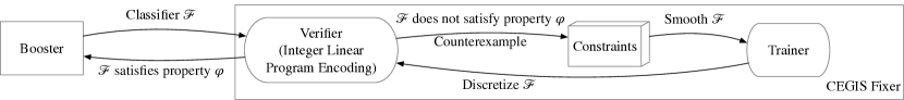
Figure 2. Booster-fixer training framework.

Then, we create the following linear constraints to ensure dependency between variables of the classifier.

Integer Constraints: We merge predicates for integer features. For example, if $x_{5}$ is an integer feature, we use the same binary variable to represent atoms $x_{5}<0.2$ and $x_{5}<0.3$.

Predicate Consistency Constraints: Predicate variables for the same feature dimension are sorted and constrained accordingly. For any $p_{i},p_{t}$ belonging to the same feature dimension with $\eta_{i}<\eta_{t}$, $x_{j}<\eta_{t}$ must be true if $x_{j}<\eta_{i}$ is true. Thus, we have $p_{i}\leq p_{t}$.

Redundant Predicate Constraints: We set redundant variables to be always 0. For example, $x_{j}<0$ is always false for a nonnegative feature.

Lastly, we use standard boolean encoding for Property Violation Constraints to verify a given property, as shown in Table 1. Each property has a pair of input and output constraints. In addition, we encode input consistency constraints for a given property.

Input Consistency Constraints: For any $x_{i}$ and $x^{\prime}_{i}$, if they are defined to be the same by the property, we set the related predicate variables $p$ and $p^{\prime}$ to have the same value.

Monotonicity: For two arbitrary inputs $x$ and $x^{\prime}$, if $x<x^{\prime}$, then there must be at least one more predicate true for $x^{\prime}$. The output constraint for (1) denotes violation to monotonically non-decreasing output, and (2) denotes violation to monotonically non-increasing output.

Stability: The input constraint says $x$ and $x^{\prime}$ are different, and the output constraint says the difference between $\mathcal{F}(x)$ and $\mathcal{F}(x^{\prime})$ are larger than the stable constant $c_{\text{stability}}$.

High Confidence: The input constraint says $x$ is classified as malicious with at least $\delta$ confidence. The output constraints says $x^{\prime}$ is classified as benign.

Redundancy: The input and output constraints are the same as high confidence property. However, we encode predicate consistency constraints differently. We set variable equality constraints such that $x_{i}=x^{\prime}_{i}$ for $i$ outside the $M$ low-cost feature groups. We encode the disjunction of the conditions that only features from the same group are changed.

Small Neighborhood: For input constraint, for each $j$, we first encode the conjunction that $x_{j}$ and $x^{\prime}_{j}$ are both within a small neighborhood interval $a_{i_{2}}-a_{i_{1}}=1$. Then, we encode the disjunction that $x_{j}$ and $x^{\prime}_{j}$ can be only within one of such intervals surrounding the predicates. The output constraint says the difference between the outputs are larger than the allowed range.

Property	Property Violation Constraints
Monotonicity	(1) In: $\sum\limits_{x}{p_{i}}\leq\sum\limits_{x^{\prime}}{p^{\prime}_{i}}+1$, Out: $\sum\limits_{x}{l_{k}*R_{k}}>\sum\limits_{x^{\prime}}{l^{\prime}_{k}*R_{k}}$
	(2) In: $\sum\limits_{x}{p_{i}}\leq\sum\limits_{x^{\prime}}{p^{\prime}_{i}}+1$, Out: $\sum\limits_{x}{l_{k}*R_{k}}<\sum\limits_{x^{\prime}}{l^{\prime}_{k}*R_{k}}$
Stability	In: $\lvert\sum\limits_{x}{p_{i}}-\sum\limits_{x^{\prime}}{p^{\prime}_{i}}\rvert\geq 1$, Out: $\lvert\sum\limits_{x}{l_{k}*R_{k}}-\sum\limits_{x^{\prime}}{l^{\prime}_{k}*R_{k}}\rvert>c_{\text{stability}}$
High Confidence	In: $\sum\limits_{x}{l_{k}*R_{k}}\geq g^{-1}(\delta)$, Out: $\sum\limits_{x^{\prime}}{l^{\prime}_{k}*R_{k}}<0$
Redundancy	Same constraints as high confidence. Diff predicate consistency constr.
Small Neighborhood	In: for each feature $j$, $x_{j}$ and $x^{\prime}_{j}$ are
	in the same interval $[\eta_{i}-\sigma_{j}*\epsilon,\eta_{i}+\sigma_{j}*\epsilon]$,
	Out: $\lvert\sum\limits_{x}{l_{k}*R_{k}}-\sum\limits_{x^{\prime}}{l^{\prime}_{k}*R_{k}}\rvert>\epsilon*c_{\text{neighbor}}$

Table 1. Property violation constraints for the verifier.

5. Training Algorithm

5.1. Framework

Figure 2 gives an overview of our booster-fixer training framework. We have two major components, a booster and a fixer, which interact with each other to train a classifier with high accuracy that satisfies the global robustness properties.

The booster increases the size of the classifier, and improves classification performance. We run $N$ boosting rounds. The classifier is a sum of logic ensembles, $\mathcal{F}(x)=\sum_{b=1}^{N}{f_{b}(x)}$, where each $f_{b}$ is a logic ensemble. In the $b$-th boosting round, the booster adds $f_{b}$ to the ensemble, proposing a candidate classifier $\sum_{i=1}^{b}{f_{i}(x)}$ (which does not need to satisfy any robustness property); then the fixer fixes property violations for this classifier. Empirically, more boosting rounds typically lead to better test accuracy after fixing the properties.

The fixer uses counterexample guided inductive synthesis (CEGIS) to fix the global robustness properties for the current classifier. We use a verifier and a trainer to iteratively train the classifier, eliminating counterexamples in each iteration, until the classifier satisfies the properties. In each CEGIS iteration, we first use the verifier to find a counterexample that violates the property. Then, we use training constraints to eliminate the counterexample. The training constraints reduce the space of candidate classifiers and make progress towards satisfying the property. We accumulate the training constraints over the CEGIS iterations, so that our classifier is guaranteed to satisfy global robustness properties when the fixer returns a solution. After we fix the global robustness properties for the classifier $\sum_{i=1}^{b}{f_{i}(x)}$, we go back to boost the next $b+1$ round, to further improve the test accuracy. We will discuss the details of our training algorithm next.

5.2. Robust Training Algorithm

Algorithm 1 presents the pseudo-code for our global robustness training algorithm. As inputs, the algorithm needs specifications of the global robustness properties $\Phi$ (Section 3.2) and a training dataset $\mathcal{D}$ to train for both robustness and accuracy. In addition, we need a booster $\mathcal{B}$ (Section 5.1), a verifier $\mathcal{V}$ (Section 4.2), a trainer $\mathcal{S}$ (described below) and a loss function $\mathcal{L}$ to run the booster-fixer rounds. We can specify the number of boosting rounds $N$. The algorithm outputs a classifier $\mathcal{F}$ that satisfies all the specified global robustness properties.

Algorithm 1 Global Robustness Property Training Algorithm

Input: Global robustness properties $\Phi$.

Training set $\mathcal{D}=\{(x^{(i)},y^{(i)})\}$. Number of boosting rounds $N$.

Input: Booster $\mathcal{B}$. Verifier $\mathcal{V}$. Trainer $\mathcal{S}$. Loss function $\mathcal{L}$.

Output: classifier $\mathcal{F}$ that satisfies all the properties in $\Phi$.

1:Initialize an empty classifier $\mathcal{F}$.

2:Initialize an empty set of constraints $\mathcal{C}$.

3:for $b=1$ to $N$ do

4:     $\mathcal{B}$ adds $f_{b}$ to $\mathcal{F}$, so that $\mathcal{F}(x)=\sum_{i=1}^{b}{f_{i}(x)}$.

5:     while $\exists\varphi_{i}\in\Phi,\mathcal{F}\not\models\varphi_{i}$ do

6:         for each $\varphi_{i}\in\Phi$ do

7:              if $\mathcal{F}\not\models\varphi_{i}$ then

8:                  Call $\mathcal{V}(\mathcal{F})$ to get a counterexample $(x,x^{\prime})$.

9:                  Call GenConstraint($x,x^{\prime}$) to get a constraint $c$.

10:                  Add $c$ to $\mathcal{C}$.

11:              end if

12:         end for

13:         if the constraints in $C$ are infeasible then

14:              return Failure.

15:         end if

16:         Update $\theta=(\alpha,\beta,R)$ using $\mathcal{S}(\alpha,\beta,R,\mathcal{D},\mathcal{C})$.

17:     end while

18:end for

19:return $\mathcal{F}$

20:

21:function GenConstraint($x,x^{\prime}$):

22:     return a constraint on $R$ that implies $\varphi(x,x^{\prime})$,

23:     when $x,x^{\prime},\alpha,\beta$ are fixed at their current values.

24:end function

25:

26:function $\mathcal{S}$($\alpha,\beta,R,\mathcal{D},\mathcal{C}$):

27:     Update $\alpha,\beta,R$ using projected gradient descent:

28:     $\alpha,\beta,R=\operatorname*{arg\ min}_{\alpha,\beta,R}\sum_{\mathcal{D}}\mathcal{L}(y,g(\mathcal{F}_{\alpha,\beta,R}(x)))$

29:     s.t. $R$ satisfies all constraints in $\mathcal{C}$

30:end function

First, our algorithm initializes an empty ensemble classifier $\mathcal{F}$ such that we can add sub-classifiers into it over the boosting rounds (Line 1). We also initialize an empty set of constraints $\mathcal{C}$ (Line 2). Then, we go through $N$ rounds of boosting in the for loop from Line 3 to Line 18. Within each boosting round $b$, the booster $\mathcal{B}$ adds a tree to the ensemble classifier, such that the current classifier is $\mathcal{F}(x)=\sum_{i=1}^{b}{f_{i}(x)}$. The fixer runs the while loop from Line 5 and Line 17. As long as the classifier does not satisfy all specified global robustness properties, we proceed with fixing the properties (Line 5). For each property, if the model does not satisfy the property, the verifier $\mathcal{V}$ produces a counterexample $(x,x^{\prime})$ (Line 8). Then, we generate a constraint $c$ that can eliminate the counterexample by calling a procedure GenConstraint$(x,x^{\prime})$ (Line 9). We add the constraint to the set $C$. If the set of constraints are infeasible, the algorithm returns failure. Otherwise, we use the trainer $\mathcal{S}$ to train the weights $\theta$ using projected gradient descent (Line 16 calls $\mathcal{S}(\alpha,\beta,R,\mathcal{D})$). We follow the gradient of the loss function w.r.t. the weights $\theta$, update the weights, and then we project the weights onto the $\ell_{2}$ norm ball centered around updated weights, subject to all constraints in $C$,. Therefore, the weights satisfy all constraints in $C$.

Generating Constraint. The GenConstraint function generates a constraint according to counterexample $(x,x^{\prime})$. We use $\mathcal{F}_{R}(x)$ to represent the equivalence class of $x$: all inputs that are classified the same as $x$, i.e., their classification score is a sum of return values for the same set of clauses as $x$. We can use constraints over $\mathcal{F}_{R}(x)$ and $\mathcal{F}_{R}(x^{\prime})$ to capture the change in the classifier’s output, to satisfy the global robustness property for all counterexamples in the equivalence class. Specifically, in Table 2, we list the constraints for five properties we have proposed. The constraints for monotonicity, stability, redundancy, and the small neighborhood properties have the same form as the output requirement specified in the corresponding property definitions. For the high confidence property, our training constraint is to bound the drop of the classification score to be no more than the $g^{-1}$ of the high confidence threshold $\delta$. This constraint aims to satisfy Property 3a (Equation 6), which then satisfies Property 3 high confidence (Lemma 1). This constraint eliminates counterexamples faster than using the constraint $\mathcal{F}_{R}(x^{\prime})\geq 0$.

Property	Training Constraints
Monotonicity	(1) $\mathcal{F}_{R}(x)\leq\mathcal{F}_{R}(x^{\prime})$
	(2) $\mathcal{F}_{R}(x)\geq\mathcal{F}_{R}(x^{\prime})$
Stability	$\lvert\mathcal{F}_{R}(x)-\mathcal{F}_{R}(x^{\prime})\rvert\leq c_{\text{stability}}$
High Confidence	$\mathcal{F}_{R}(x)-\mathcal{F}_{R}(x^{\prime})<g^{-1}(\delta)$
Redundancy	Same as high confidence.
Small Neighborhood	$\lvert\mathcal{F}_{R}(x)-\mathcal{F}_{R}(x^{\prime})\rvert\leq\epsilon*c_{\text{neighbor}}$

Table 2. Constraints used for the training algorithm.

CLN Trainer. Within the fixer, we use Continuous Logic Networks (CLN) (Ryan et al., 2020) to train the classifier to satisfy all constraints in $C$. If we directly enforce constraints over the weights of the classifier, the structure and weights will not have good accuracy. We want to use gradient-guided optimization to preserve accuracy of the classifier while satisfying the constraints. Since our discrete ensemble classifier is non-differentiable, we first use CLN to smooth the logic ensemble. Following Ryan et al. (Ryan et al., 2020), we use a shifted and scaled sigmoid function to smooth the inequalities, product t-norm to smooth conjunctions. To train the smoothed model, we use binary cross-entropy loss as the loss function $\mathcal{L}$ for classification, and minimize the loss using projected gradient descent according to the constraints $C$. After training, we discretize the model back to logic ensemble for prediction, so we can verify the robustness properties. Note that although our training constraints $C$ are only related to the returned activation values of the clauses (Table 2), the learnable parameters of atoms may change as well due to the projection (See Appendix A for an example). In some cases, the structure of the atom can change as well. For example, if an atom $x_{0}<5$ is trained to become $-0.5*x_{0}<2$, this changes the inequality of the atom.

5.2.1. Supported Properties.

Our framework can handle any global robustness property $\varphi$ of the form $\forall x_{1},\dots,x_{k}.\mu(x_{1},\dots,x_{k})\implies\nu(\mathcal{F}(x_{1}),\dots,\mathcal{F}(x_{k}))$ where the set of values $\{(y_{1},\dots,y_{k}):\nu(y_{1},$ $\dots,y_{k})\}$ is a convex set, as then we can project the classifier weights accordingly (line 27 to line 29 in Algorithm 1). For example, for the monotonicity property, $k=2$, $\mu(x_{1},x_{2})\coloneqq x_{1}\leq x_{2}$, and $\nu(\mathcal{F}(x_{1}),\mathcal{F}(x_{2}))\coloneqq\mathcal{F}(x_{1})\leq\mathcal{F}(x_{2})$. This class includes but is not limited to all global robustness properties with arbitrary linear constraints on the outputs of the classifier.

5.2.2. Algorithm Termination.

Algorithm 1 is guaranteed to terminate. When the algorithm terminates, if it finds a classifier, the classifier is guaranteed to satisfy the properties. However, there is no guarantee that it will find a classifier (line 14 of Algorithm 1 returns Failure), but empirically our algorithm can find an accurate classifier that satisfies all the specified properties, as shown in the results in Section 6.3.

6. Evaluation

Dataset	Property	Specification
Cryptojacking	-	Low-cost features: whether a website uses one of the hash functions on the list.
	Monotonicity	Increasing: all features
	Stability	All features are stable. Stable constant = $0.1$
	High Confidence	$\delta=0.98$
	Small Neighborhood	$\epsilon=0.2,c=0.5$
	Combined	Monotonicity, stability, high confidence, and small neighborhood
Twitter Spam Accounts	-	Low-cost features: LenScreenName ($\geq 5$ char), LenProfileDescription, NumTweets, NumDailyTweets,
		TweetLinkRatio, TweetUniqLinkRatio, TweetAtRatio, TweetUniqAtRatio.
	Monotonicity	Increasing: LenScreenName, NumFollowings, TweetLinkRatio, TweetUniqLinkRatio
		Decreasing: AgeDays, NumFollowers
	Stability	Low-cost features are stable. Stable constant = $8$.
	High Confidence	$\delta=0.98$. Attacker is allowed to perturb any one of the low-cost features, but not multiple ones.
	Redundancy	$\delta=0.98,M=2$, any 2 in 4 groups satisfy redundancy: 1) LenScreenName ($\geq 5$ char), LenProfileDescription
		2) NumTweets, NumDailyTweets 3) TweetLinkRatio, TweetUniqLinkRatio 4) TweetAtRatio, TweetUniqAtRatio
	Small Neighborhood	$\epsilon=0.1,c=50$
	Combined	Monotonicity, stability, high confidence, redundancy, and small neighborhood
Twitter Spam URLs	-	Low-cost features: Mention Count, Hashtag Count, Tweet Count, URL Percent.
	Monotonicity	Increasing: 7 shared resources features. EntryURLid, AvgURLid, ChainWeight,
		CCsize, MinRCLen, AvgLdURLDom, AvgURLDom
	Stability	Low-cost features are stable. Stable constant = $8$.
	High Confidence	$\delta=0.98$. Attacker is allowed to perturb any one of the low-cost features, but not multiple ones.
	Small Neighborhood	$\epsilon=1.5,c=10$

Table 3. Global robustness property specifications for three datasets.

6.1. Datasets and Property Specifications

We evaluate how well our training technique works on three security datasets of different scale: detection of cryptojacking (Kharraz et al., 2019), Twitter spam accounts (Lee et al., 2011), and Twitter spam URLs (Kwon et al., 2017). Table 5 shows the size of the datasets. In total, the three datasets have 4K, 40K, and 422,672 data points respectively. Appendix D lists all the features for the three datasets. We specify global robustness properties for each dataset (Table 3) based on our analysis of what kinds of evasion strategies might be relatively easy and inexpensive for attackers to perform.

Monotonic Directions. To specify monotonicity properties, we use two types of security domain knowledge, suspiciousness and economic cost. We specify a classifier to be monotonically increasing for a feature if, (1) an input is more suspicious as the feature value increases, or, (2) a feature requires a lot of money to be decreased but easier to be increased, such that we force the attackers to spend more money in order to reduce the classification score. Similarly, we specify a classifier to be monotonically decreasing along a feature dimension by analyzing these two aspects.

6.1.1. Cryptojacking

Crytpojacking websites are malicious webpages that hijack user’s computing power to mine cryptocurrencies. Kharraz et al. (Kharraz et al., 2019) collected cryptojacking website data from 12 families of mining libraries. We randomly split the dataset containing 2000 malicious websites and 2000 benign websites into 70% training set and 30% testing data. In total, there are 2800 training samples and 1200 testing samples. We use the training set as the validation set.

Low-cost feature. Among all features, only the hash function feature is low cost to change. The attacker may use a hash function not on the list, or may construct aliases of the hash functions to evade the detection. Since the other features are related to usage of standard APIs or essential to running high performance cryptocurrency mining code, they are not trivial to evade.

Monotonicity. We specify all features to be monotonically increasing. Kharraz et al. (Kharraz et al., 2019) proposed seven features to classify cryptojacking websites. A website is more suspicious if any of these features have larger values. Specifically, cryptojacking websites prefer to use WebSocket APIs to reduce network communication bandwidth, use WebAssembly to run mining code faster, runs parallel mining tasks, and may use a list of hash functions. Also, if a website uses more web workers, has higher messageloop load, and PostMessage event load, it is more suspicious are performing some heavy load operations such as coin mining.

Stability. Since this is a small dataset, we specify all features to be stable, with stable constant $0.1$.

High Confidence. We use high confidence threshold $0.98$.

Small Neighborhood. We specify $\epsilon=0.2,c=0.5$. Each feature is allowed to be perturbed by up to $20\%$ of its standard deviation, and the output of the classifier is bounded by $0.01$.

6.1.2. Twitter Spam Accounts

Lee et al. (Lee et al., 2011) used social honeypot to collect information about Twitter spam accounts, and randomly sampled benign Twitter users. We reimplement 15 of their proposed features, including account age, number of following, number of followers, etc., with the entire list in Table 11, Appendix D. We randomly split the dataset into 36,000 training samples and 4,000 testing samples, and we use the training set as validation set.

Dataset	Training set size	Test set size	Validation set size	# of features
Cryptojacking (Kharraz et al., 2019)	2800	1200	Train	7
Twitter Spam Accounts (Lee et al., 2011)	36,000	4,000	Train	15
Twitter Spam URLs (Kwon et al., 2017)	295,870	63,401	63,401	25

Table 4. The three datasets we use to evaluate our methods. For cryptojacking and Twitter spam account datasets, we use the training set as the validation set.

# Char	Price
$\leq 4$	$1,598.09
$\geq 5$	$298.40
Unspecified	$147.62

Table 5. Average price of for-sale Twitter accounts with different number of characters for the username.

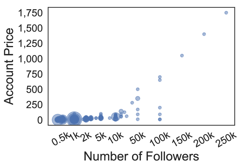
Figure 3. Price ($) of for-sale Twitter accounts with different number of followers.

Economic Cost Measurement Study. We have crawled and analyzed 6,125 for-sale Twitter account posts from an underground forum to measure the effect of LenScreenName and NumFollowers on the prices of the accounts.

• LenScreenName. Accounts with at most 4 characters are deemed special in the underground forum, usually on sale with a special tag ‘3-4 Characters’. Table 5 shows that the average price of accounts with at most 4 characters is five times the price of accounts with more characters or unspecified characters. More measurement results are in Appendix C.1.

• NumFollowers. We measure the account price distribution according to different tiers of followers indicated in the underground forum, from 500, 1K, 2K up to 250K followers. As shown in Figure 3, the account prices increase as the number of followers increases.

Low-cost Features. We identify 8 low-cost features in total. Among them, two features are related to the user profile, LenScreenName and LenProfileDescription. According to our economic cost measurement study, accounts with user names up to 4 characters are considered high cost to obtain. Therefore, we specify LenScreenName with at least 5 characters to be low cost feature range. The other four low-cost features are related to the tweet content, since they can be trivially modified by the attacker: NumTweets, NumDailyTweets, TweetLinkRatio, TweetUniqLinkRatio, TweetAtRatio, and TweetUniqAtRatio.

Monotonicity. We specify two features to be monotonically increasing, and two features to be monotonically decreasing, based on domain knowledge about suspicious behavior and economic cost measurement studies.

Increase in suspiciousness: Spammers tend to follow a lot of people, expecting social reciprocity to gain followers for spam content, so large NumFollowings makes an account more suspicious. If an account sends a lot of links (TweetLinkRatio and TweetUniqLinkRatio), it also becomes more suspicious.

Decrease in suspiciousness: Since cybercriminals are constantly trying to evade blocklists, if an account is newly registered with a small AgeDays value, it is more suspicious.

Increase in economic cost: Since the attacker needs to spend more money to obtain Twitter accounts with very few characters, we specify the LenScreenName to be monotonically increasing,

Decrease in economic cost: Since it is expensive for attackers to obtain more followers, we specify the NumFollowers feature to be monotonically decreasing.

Stability. We specify all the low-cost features to be stable, with stable constant 8.

High Confidence. We allow the attacker to modify any one of the low cost features individually, but not together. We use a high confidence prediction threshold $0.98$.

Redundancy. Among the 8 low-cost features, we identify four groups, where each group has one feature that counts an item in total, and one other feature that counts the same item in a different granularity (daily or unique count). We specify that any two groups are redundancy of each other ($M=2$) with $\delta=0.98.$

Small Neighborhood. We specify $\epsilon=0.1,c=50$. The attacker can change each feature up to $10\%$ of its standard deviation value, and the classifier output change is bounded by $5$.

	Performance					Global Robustness Properties
Model	TPR	FPR	Acc	AUC	F1	Monotonicity	Stability	High Confidence	Redundancy	Small Neighborhood
	(%)	(%)	(%)
Cryptojacking Detection
XGB	100	0.3	99.8	.99917	.998	✘	✘	✔	N/A	✘
Neural Network	100	0.2	99.9	.99997	.999	✘	✘	?	N/A	✘
Models with Monotonicity Property
Monotonic XGB	99.8	0.3	99.8	.99969	.998	✔	✘	✔	N/A	✘
Nonnegative Linear	97.7	0.2	98.8	.99987	.988	✔	✘	✘	N/A	✘
Nonnegative Neural Network	99.7	0.2	99.8	.99999	.998	✔	✘	?	N/A	✘
Generalized UMNN	99.8	0.2	99.8	.99998	.998	✔	✘	?	N/A	✘
DL2 Models with Local Robustness Properties, trained using PGD attacks
DL2 Monotoncity	99.7	0.2	99.8	.99999	.998	✘	✘	?	N/A	✘
DL2 Stability	99.8	0.8	99.5	.99987	.995	✘	✘	✘	N/A	✘
DL2 High Confidence	99.7	0.2	99.8	.99999	.998	✘	✘	?	N/A	✘
DL2 Small Neighborhood	99.8	0.3	99.8	.99999	.998	✘	✘	?	N/A	✘
DL2 Combined	99.3	0.2	99.6	.99985	.996	✘	✘	✘	N/A	✘
Our Models with Global Robustness Properties
Logic Ensemble Monotoncity	100	0.3	99.8	.99999	.998	✔	✘	✔	N/A	✘
Logic Ensemble Stability	100	0.3	99.8	.99831	.998	✘	✔	✔	N/A	✔
Logic Ensemble High Confidence	100	0.3	99.8	.99980	.998	✘	✘	✔	N/A	✘
Logic Ensemble Small Neighborhood	100	0.3	99.8	.99961	.998	✘	✔	✔	N/A	✔
Logic Ensemble Combined	100	3.2	98.4	.99831	.985	✔	✔	✔	N/A	✔

Table 6. Results for training cryptojacking classifier with global robustness properties, compared to baseline models. N/A: property not specified. ✔: verified to satisfy the property. ✘: verified to not satisfy the property. $?$: unknown.

6.1.3. Twitter Spam URLs

Kwon et al. (Kwon et al., 2017) crawled 15,828,532 tweets by 1,080,466 users. They proposed to use URL redirection chains and and graph related features to classify spam URL posted on Twitter. We obtain their public dataset and re-extract 25 features according to the description in the paper. We extract four categories of features. (1) Shared resources features capture that the attacker reuse resources such as hosting servers and redirectors. (2) Heterogeneity-driven features reflect that attack resources may be heterogeneous and located around the world. (3) Flexibility-driven features capture that attackers use different domains and initial URLs to evade blocklists. (4) Tweet content features measure the number of special characters, tweets, percentage of URLs made by the same user. This is the largest dataset in our evaluation, containing 422,672 samples in total. We randomly split the dataset into $70\%$ training, $15\%$ testing, and $15\%$ validation sets.

Low-cost Features. We specify four tweet content related features to be low cost, since the attacker can trivially modify the content. They are, Mention Count, Hashtag Count, Tweet Count, and URL percent in tweets. All the other features are high cost, since they are related to the graph of redirection chains, which cannot be easily controlled by the attacker. Redirection chains form the traffic distribution systems in the underground economy, where different cybercriminals can purchase and re-sell the traffic (Li et al., 2013; Goncharov, [n.d.]). Thus graph-related features are largely outside the control of a single attacker, and are not trivial to change.

Monotonicity. Based on feature distribution measurement result, we specify that 7 shared resources-driven features are monotonically increasing, as shown in Table 3. Example measurement result is in Appendix C.2.

Stability. We specify low-cost features to be stable, with stable constant 8.

High Confidence. We use a high confidence prediction threshold $0.98$. Attacker is allowed to perturb any one of the low-cost features, but not multiple ones.

Small Neighborhood. We specify $\epsilon=1.5,c=10$, which means that the attacker can change each feature up to $1.5$ times of its standard deviation, and the classifier output change is bounded by $15$.

6.2. Baseline Models

6.2.1. Experiment Setup

We compare against three types of baseline models, (1) tree ensemble and neural network that are not trained using any properties, (2) monotonic classifiers, and (3) neural network models trained with local robustness versions of our properties.

We train the following monotonic classifiers: monotonic gradient boosted decision trees using XGBoost (Monotonic XGB), linear classifier with nonnegative weights trained using logistic loss (Nonnegative Linear), nonnegative neural network, and generalized unconstrained monotonic neural network (UMNN) (Wehenkel and Louppe, 2019). To evaluate against models with other properties, we train local versions of our properties using DL2 (Fischer et al., 2019), which uses adversarial training.

Malicious Class Gradient Weight. Since the Twitter spam account dataset (Lee et al., 2011) is missing some important features, we could not reproduce the exact model performance stated in the paper. Instead, we get 6% false positive rate. We contacted the authors but they don’t have the missing data. Therefore, we tune the weight for the gradient of the malicious class in order to maintain low false positive rate for the models. We use line search to find the best weight from 0.1 to 1, which increments by 0.1. We find that using 0.2 to weigh the gradient of the malicious class can keep the training false positive rate around 2% for this dataset. For the other two datasets, we do not weigh the gradients for different classes.

Linear Classifier. The nonnegative linear classifier is a linear combination of input features with nonnegative weights, trained using logistic loss. If a feature is specified to be monotonically decreasing, we weigh the feature by -1 at input.

XGBoost Models. For the XGB model and Monotonic XGB model, we specify the following hyperparameters for three datasets. We use 4 boosting round, max depth 4 per tree to train the cryptojacking classifier, and 10 boosting rounds, max depth 5 to train Twitter spam account and Twitter spam URL classifiers.

Neural Network Models. The neural networks without any robustness properties as well as the nonnegative-weights networks have two fully connected layers, each with 200, 500, and 300 ReLU units for Cryptojacking, Twitter spam account, and Twitter Spam URL detection respectively. The generalized UMNNs, on the other hand, are positive linear combinations of multiple UMNN each with two fully connected layers and 50, 100, 100 ReLU nodes for each single monotonic feature.

We also use DL2 to train neural networks as baselines, which can achieve local robustness properties using adversarial training. All the DL2 models share the same architectures as the regular neural networks and the training objectives is to minimize the loss of PGD adversarial attacks (Kurakin et al., 2017) that target the robustness properties. We use 50 iterations with step sizes equal to one sixth of the allowable perturbation ranges for PGD attacks in the training process. For testing, we use the same PGD iterations and step sizes but with 10 random restarts.

For all the baseline neural networks mentioned above, we train 50 epochs to minimize binary cross-entropy loss on training datasets using Adam optimizer with learning rate 0.01 and piecewise learning rate scheduler.

6.2.2. Global Robustness Property Evaluation

To evaluate whether the baseline models have obtained global robustness properties, we use our Integer Linear Programming verifier to verify the XGB and linear models. For neural network models, we use PGD attacks to maximize the loss function for the property, as described in Section 6.2.1.

Table 6 and Table 8 show the results of evaluating global robustness properties for the baseline models. For neural network models, if the PGD attack has found counterexample for the property, we consider that the network does not satisfy the property. Otherwise, we use “?” to mark it as unknown/unverified.

Result 1: Monotonic XGB and generalized UMNN have the best true positive rate (TPR) among monotonic classifiers. For the two relatively large datasets, the performance of monotonic XGB and generalized UMNN are much better than nonnegative-weights models. For Twitter spam account detection, the TPR of monotonic XGB is $16.6\%$ higher than the nonnegative linear classifier.

Result 2: Some baseline models naturally satisfy a few global robustness properties. The monotonic XGB model for crytpojacking detection satisfies the high confidence property, because it does not use the low-cost feature “hash function” in the tree structure. In comparison, our technique can train logic ensemble classifiers to satisfy the high confidence property but still use the low-cost feature to improve accuracy. Also, the nonnegative linear classifier for Twitter spam account detection satisfies the small neighborhood property, but it has only $70.1\%$ TPR. Linear classifiers are known to be robust against small changes in input, however they have poor performance for many datasets.

Result 3: DL2 models cannot obtain global robustness. We found counterexamples for all DL2 models for Twitter spam URL detection, using PGD attacks over the property constraint loss, and most models trained with cryptojacking and Twitter spam account detection datasets. If the PGD attack fails to find a counterexample, it does not mean that the model is verified to have the global property. There are always stronger attacks that may find counterexamples, as is often observed with adversarially trained models.

6.3. Robust Logic Ensembles

6.3.1. Training Algorithm Implementation

We implement our booster-fixer framework as the following. We use gradient boosting from XGBoost (Chen and Guestrin, 2016) as the booster. Within each round, we use the booster to add one tree to the existing classifier, and encode the classifier as the logic ensemble. This gives the fixer the structure of clauses and weights ($\alpha,\beta,R$ ) as the starting classifier with high accuracy.

To implement the verifier in the fixer, we use APIs from Gurobi (gur, [n.d.]) to encode the integer linear program with boolean variables and property violation constraints, and then call the Gurobi solver to verify the global robustness properties of the logic ensemble. If the solver returns that the interger linear program is infeasible, the classifier is verified to satisfy the property. Otherwise, we construct a counterexample according to solutions for the boolean variables. For the trainer, we use PyTorch to implement the smoothed classifier as Continuous Logic Networks (Ryan et al., 2020; Yao et al., 2020). Then, we use quadratic programming to implement projected gradient descent. We compute the updated weights by minimizing the $\ell_{2}$ norm between the initial weights and the convex set defined by the training constraints. We implement the mini-batch training for the smoothed classifier, where we can specify the batch size. After one epoch of training, we discretize the classifier to the logic ensemble encoding for the verifier to verify the property again. We also implement a few heuristics to speed up the time for the verifier to generate counterexamples, with details described in Appendix E.

Dataset	Median Training Time
Cryptojacking	25 min
Twitter Spam Account	29 hours
Twitter Spam URL	3 days

Table 7. Median training time for Logic Ensemble models.

	Performance					Global Robustness Properties
Model	TPR	FPR	Acc	AUC	F1	Monotonicity	Stability	High Confidence	Redundancy	Small Neighborhood
	(%)	(%)	(%)
Twitter Spam Account Detection
XGB	87.0	2.3	92.2	.98978	.920	✘	✘	✘	✘	✘
Neural Network	86.4	2.5	91.8	.98387	.915	✘	✘	✘	✘	✘
Models with Monotonicity Property
Monotonic XGB	86.7	2.7	91.9	.98865	.916	✔	✘	✘	✘	✘
Nonnegative Linear	70.1	2.4	83.5	.95321	.814	✔	✘	✘	✘	✔
Nonnegative Neural Network	78.3	2.5	87.6	.96723	.867	✔	✘	✘	✘	✘
Generalized UMNN	86.0	3.9	90.9	.97324	.907	✔	✘	✘	✘	✘
DL2 Models with Local Robustness Properties, trained using PGD attacks
DL2 Monotoncity	83.2	2.6	90.1	.97800	.896	✘	✘	✘	✘	✘
DL2 Stability	86.1	3.3	91.3	.98029	.910	✘	?	✘	✘	✘
DL2 High Confidence	82.8	2.6	89.9	.98056	.894	✘	✘	✘	✘	✘
DL2 Redundancy	83.9	3.1	90.2	.97898	.898	✘	✘	?	✘	✘
DL2 Small Neighborhood	88.3	3.5	92.2	.98086	.921	✘	✘	✘	✘	✘
DL2 Combined	83.8	3	90.2	.97738	.898	✘	✘	✘	✘	?
Our Models with Global Robustness Properties
Logic Ensemble Monotoncity	83.2	3.2	89.8	.97297	.894	✔	✘	✘	✘	✘
Logic Ensemble Stability	86.0	2.1	91.8	.98479	.915	✘	✔	✘	✘	✘
Logic Ensemble High Confidence	86.1	2.6	91.6	.98311	.913	✘	✔	✔	✘	✘
Logic Ensemble Redundancy	85.5	3.2	91.0	.98166	.907	✘	✔	✔	✔	✘
Logic Ensemble Small Neighborhood	83.9	2.5	90.5	.98325	0.901	✘	✔	✘	✘	✔
Logic Ensemble Combined	81.6	2.4	89.4	.98142	.888	✔	✔	✔	✔	✔
Twitter Spam URL Detection
XGB	99.0	1.5	98.7	.99834	.986	✘	✘	✘	N/A	✘
Neural Network	98.8	2.9	97.9	.99735	.977	✘	✘	✘	N/A	✘
Models with Monotonicity Property
Monotonic XGB	99.4	1.7	98.8	.99848	.986	✔	✘	✘	N/A	✘
Nonnegative Linear	93.2	18.6	86.7	.90218	.861	✔	✘	✘	N/A	✘
Nonnegative Neural Network	98.0	6.9	95.3	.98511	.949	✔	✘	✘	N/A	✘
Generalized UMNN	98.8	2.6	98.0	.99732	.977	✔	✘	✘	N/A	✘
DL2 Models with Local Robustness Properties, trained using PGD attacks
DL2 Monotoncity	98.9	3.0	97.9	.99694	.976	✘	✘	✘	N/A	✘
DL2 Stability	99.0	3.0	97.9	.99706	.977	✘	✘	✘	N/A	✘
DL2 High Confidence	99.5	4.6	97.2	.99696	.969	✘	✘	✘	N/A	✘
DL2 Small Neighborhood	99.1	3.0	97.9	.99720	.977	✘	✘	✘	N/A	✘
Our Models with Global Robustness Properties
Logic Ensemble Monotoncity	96.3	3.5	96.4	.98549	.960	✔	✘	✘	N/A	✘
Logic Ensemble Stability	92.9	3.3	95.0	.98180	.943	✘	✔	✘	N/A	✔
Logic Ensemble High Confidence	97.6	5.4	95.9	.98646	.955	✘	✔	✔	N/A	✘
Logic Ensemble Small Neighborhood	97.1	2.8	97.1	.99338	.968	✘	✘	✘	N/A	✔

Table 8. Results for training Twitter account classifier and Twitter spam URL classifier with global robustness properties, compared to baseline models. N/A: property not specified. ✔: verified to satisfy the property. ✘: verified to not satisfy the property. $?$: unknown.

6.3.2. Experiment Setup.

For the cryptojacking dataset, we boost 4 rounds, each adding a tree with max depth 4. For the other two datasets, we boost 10 rounds, with max tree depth 5, except that we only boost 6 rounds when training the Twitter spam account classifier with all five properties. During CLN training, we keep track of the discrete classifier at each stage, including all the inequalities and conjunctions. When we need to smooth the classifier, we use shifted and scaled sigmoid function to smooth the inequality, with temperature $\frac{1}{500}$, shift by $0.01$, and product t-norm to smooth the conjunctions, to closely approximate the discrete classifier. The updated weights from gradient-guided training can be directly used for the discrete classifier. To discretize the model, we simply do not apply the sigmoid function and the product t-norm. We use the Adam optimizer with learning rate $0.001$ and decay $0.95$, to minimize binary cross-entropy loss using gradient descent. For the crytpojacking dataset, we use mini-batch size 1; for the other two larger datasets, we use mini-batch size 1024. After boosting all the rounds, we choose the model with the highest validation AUC. Empirically, our algorithm converges well to an accurate classifier that satisfies the specified properties.

6.3.3. Global Robustness Property Evaluation

We train 15 logic ensemble models in total for the three datasets, each satisfying the specified global robustness properties, shown in Table 6 and Table 8. We use our Integer Linear Program verifier (Section 4.2) to verify the properties for all models.

Training Overhead. Similar to most existing robust machine learning training strategies, training a verifiably robust model is significantly slower than training a non-robust model. We show the median training time for Logic Ensemble models in Table 7. Training non-robust XGBoost models takes one minute. However, computation is usually cheap and the tradeoff for getting more robustness in exchange for more computation is common across robust machine learning techniques. Next, we discuss our key results.

Result 4: Our monotonic models have comparable or better performance than existing methods. Our Logic Ensemble Monotonicity models have higher true positive rate and AUC than the Nonnegative Linear classifiers for all three datasets, and we also achieve better performance than the Nonnegative Neural Network models for the cryptojacking detection and Twitter account detection datasets. Monotonic XGB outperforms our Logic Ensemble Monotonic models, but we still have comparable performance. For example, for the Twitter spam account detection, our Logic Ensemble Monotonicity model has $3.5\%$ lower true positive rate (TPR), and $0.5\%$ higher false positive rate (FPR) than the Monotonic XGB model.

Result 5: Our models have moderate performance drop to obtain an individual property. For cryptojacking detection, enforcing each property does not decrease TPR at all, and only increases FPR by $0.1\%$ compared to the baseline neural network model (Table 6). For Twitter spam account detection, logic ensemble models that satisfy one global robustness property decrease the TPR by at most $3.8\%$, and increase the FPR by at most $0.9\%$, compared to the baseline XGB model (Table 8). For Twitter spam URL detection, within monotonicity, stability, and small neighborhood properties, enforcing one property for the classifier can maintain high TPR (from $92.9\%$ to $97.6\%$) and low FPR (from $2.8\%$ to $5.4\%$, Table 8). For example, the Logic Ensemble High Confidence model decreases the TPR by $1.4\%$ and increases the FPR by $3.9\%$, compared to the baseline XGB model. This model utilizes the low-cost features to improve the prediction accuracy. If we only use high-cost features to train a tree ensemble with the same capacity (10 rounds of boosting), we can only achieve $79.9\%$ TPR and $0.96075$ AUC. In comparison, our Logic Ensemble High Confidence model has $97.6\%$ TPR and $0.98646$ AUC. Results regarding hyperparameters are discussed in Appendix F.

Result 6: Training a classifier with one property sometimes obtains another property. Table 6 shows that all cryptojacking Logic Ensemble classifiers that were enforced with only one property, have obtained at least one other property. For example, the Logic Ensemble Stability model has obtained small neighborhood property, and vice versa. Since we specify all features to be stable for this dataset, the stability property is equivalent to the global Lipschitz property under $L_{0}$ distance. On the other hand, we define the small neighborhood property with a new distance. This shows that enforcing robustness for one property can generalize the robustness to a different property. More results are discussed in Appendix G.

Result 7: We can train classifiers to satisfy multiple global robustness properties at the same time. We train a cryptojacking classifier with four properties, and a Twitter spam account classifier with five properties. For cryptojacking detection, the Logic Ensemble Combined model maintains the same high TPR, and only increases the FPR by $3\%$ compared to the baseline neural network model (Table 6). For Twitter spam account detection, the Logic Ensemble Combined model that satisfies all properties only decreases the TPR by $5.4\%$ and increases the FPR by $0.1\%$, compared to the baseline XGB model with no property (Table 8). More results are discussed in Appendix H.

7. Related Work

Program Synthesis. Solar-Lezama et al. (Solar-Lezama et al., 2006) proposed counterexample guided inductive synthesis (CEGIS) to synthesize finite programs according to specifications of desired functionalities. The key idea is to iteratively generate a proposal of the program and check the correctness of the program, where the checker should be able to generate counterexamples of correctness to guide the program generation process. The general idea of CEGIS has also been used to learn recursive logic programs (e.g., as static analysis rules) (Cropper et al., 2020; Albarghouthi et al., 2017; Si et al., 2018; Raghothaman et al., 2019). We design our fixer following the general form of CEGIS.

Local Robustness. Many techniques have been proposed to verify local robustness (e.g., $\ell_{p}$ robustness) of neural networks, including customized solvers (Katz et al., 2017; Tjeng et al., 2017; Huang et al., 2017; Katz et al., 2019) and bound propagation based verification methods (Li et al., 2020; Wong and Kolter, 2018; Raghunathan et al., 2018b; Wang et al., 2018c, b; Wang et al., 2021; Xu et al., 2021; Singh et al., 2019b, c; Balunović et al., 2019; Singh et al., 2019a; Müller et al., 2021a, b; Zhang et al., 2018; Boopathy et al., 2019; Weng et al., 2018a; Salman et al., 2019b). Bound propagation verifiers can also be applied in robust optimization to train the models with certified local robustness (Wong et al., 2018; Zhang et al., 2020; Mirman et al., 2018; Wang et al., 2018a; Boopathy et al., 2021; Li et al., 2019b; Zhang and Evans, 2019; Chen et al., 2020). Randomized smoothing (Cohen et al., 2019b; Jia et al., 2019; Lecuyer et al., 2019; Salman et al., 2019a; Yang et al., 2020; Li et al., 2019a) is another technique to provide probabilistic local robustness guarantee. Several methods have been proposed to utilize the local Lipshitz constant of neural networks for verification (Weng et al., 2018a, b; Hein and Andriushchenko, 2017), and constrain or use the local Lipshitz bounds to train robust networks (Szegedy et al., 2013; Cisse et al., 2017; Cohen et al., 2019a; Anil et al., 2019; Pauli et al., 2021; Qin et al., 2019; Finlay and Oberman, 2021; Lee et al., 2020; Gouk et al., 2021; Singla and Feizi, 2019; Farnia et al., 2018).

Global Robustness. Fischer et al. (Fischer et al., 2019) and Melacci et al. (Melacci et al., 2020) proposed global robustness properties for image classifiers using universally quantified statements. Both of their techniques smooth the logic expression of the property into a differentiable loss function, and then use PGD attacks (Kurakin et al., 2017) to minimize the loss. They can train neural networks to obtain local robustness, but cannot obtain verified global robustness. ART (Lin et al., 2020) proposed an abstraction refinement strategy to train provably correct neural networks. The model satisfies global robustness properties when the correctness loss reaches zero. However, in practice their correctness loss did not converge to zero. Leino et al. (Leino et al., 2021) proposed to minimize global Lipschitz constant to train globally-robust neural networks, but they can only verify one global property that abstains on non-robust predictions.

Monotonic Classifiers. Many methods have been proposed to train monotonic classifiers (Wehenkel and Louppe, 2019; Incer et al., 2018; Archer and Wang, 1993; Daniels and Velikova, 2010; Kay and Ungar, 2000; Ben-David, 1995; Duivesteijn and Feelders, 2008; Feelders, 2010; Gupta et al., 2016). Recently, Wehenkel et al. (Wehenkel and Louppe, 2019) proposed unconstrained monotonic neural networks, based on the key idea that a function is monotonic as long as its derivative is nonnegative. This has increased the performance of monotonic neural network significantly compared to enforcing nonnegative weights. Incer et al. (Incer et al., 2018) used monotone constraints from XGBoost to train monotonic malware classifiers. XGBoost enforces monotone constraints for the left child weight to be always smaller (or greater) than the right child, which is a specialized method and does not generalize to other global robustness properties.

Discrete Classifier and Smoothing. Friedman et al. (Friedman et al., 2008) proposed rule ensemble, where the each rule is a path in the decision tree, and they used regression to learn how to combine rules. Our logic ensemble is more general such that the clauses do not have to form a tree structure. We only take rules from trees as the starting classifier to fix the properties. Kantchelian et al. (Kantchelian et al., 2016) proposed the mixed integer linear program attack to evade tree ensembles by perturbing a concrete input. In comparison, our integer linear program verifier has only integer variables, and represents all inputs symbolically. Continuous Logic Networks was proposed to smooth SMT formulas to learn loop invariants (Ryan et al., 2020; Yao et al., 2020). In this paper, we apply the smoothing techniques to train machine learning classifiers.

8. Conclusion

In this paper, we have presented a novel booster-fixer training framework to enforce new global robustness properties for security classifiers. We have formally defined six global robustness properties, of which five are new. Our training technique is general, and can handle a large class of properties. We have used experiments to show that we can train different security classifiers to satisfy multiple global robustness properties at the same time.

9. Acknowledgements

We thank the anonymous reviewers for their constructive and valuable feedback. This work is supported in part by NSF grants CNS-18-50725, CCF-21-24225; generous gifts from Open Philanthropy, two Google Faculty Fellowships, Berkeley Artificial Intelligence Research (BAIR), a Capital One Research Grant, a J.P. Morgan Faculty Award; and Institute of Information & communications Technology Planning & Evaluation (IITP) grant funded by the Korea government(MSIT) (No.2020-0-00153). Any opinions, findings, conclusions, or recommendations expressed herein are those of the authors, and do not necessarily reflect those of the US Government, NSF, Google, Capital One, J.P. Morgan, or the Korea government.

Figure 4. One CEGIS iteration to train stability property for the Twitter account classifier. We specify the classifier’s output score to change at most by one when the URLRatio feature is arbitrarily perturbed. Multiple weights of the classifiers are updated by gradient-guided optimization, and the classifier after training no longer forms a tree structure.

Appendix A Stability for Twitter Account Classifier

To classify Twitter accounts that broadcast spam URLs, we can use the number of followers and the ratio of posted URLs over total number of tweets as features (Lee et al., 2011). It is hard for spammers to obtain large amount of followers, and they are likely to post more URLs than benign users. We specify the URLRatio feature to be stable, such that arbitrarily changing the feature will not change the classifier’s output by more than 1.

Figure 4 shows one CEGIS iteration to train the stability property. The starting classifier is a decision tree. For example, “$1.0*\texttt{URLRatio}<0.285\land 1.0*\texttt{followers}<1429.5\rightarrow-1.71$” means that if the URLRatio and the number of followers both satisfy these inequalities, the clause is true and returns $-1.71$, value of the variable $R_{0}$. Otherwise, the clause returns $0$. We take the sum of return values from all clauses to be the classification score. One CEGIS iteration goes through the following four steps.

Step ①: We ask the verifier whether the URLRatio feature is stable. If the verifier can verify the stability property, we stop here. If not, the verifier generates a counterexample that violates the property. Here, the counterexample shows that if the number of followers is 2000, and if the URLRatio feature changes from $0.9$ to $0.223$, the classifier’s output changes by 1.31, which violates the stability property.

Step ②: Using the sum of true clauses for each input, we represent $x,x^{\prime}$ as $\mathcal{F}_{R}(x)=R_{3}$, and $\mathcal{F}_{R}(x^{\prime})=R_{1}$.

Step ③: We construct the constraint to eliminate the counterexample. In this case, we want the difference between the output for $x$ and the output for $x^{\prime}$ to be bounded by 1, i.e., $\lvert R_{3}-R_{1}\rvert\leq 1$. Then, we smooth the classifier using CLN (Ryan et al., 2020; Yao et al., 2020), train the weights using projected gradient descent with the constraint. After one epoch, we have updated the classifier in the rightmost box of Figure 4. The red weights of the model are updated by gradient descent. Note that the classifier no longer follows a tree structure.

Lastly, we repeat this process until the classifier is verified to satisfy the property (Step ④). In this example, the updated classifier still does not satisfy stability, and we will go through more CEGIS iterations to update it.

Appendix B Proof

Lemma 1.

If a classifier satisfies Property 3a, then it also satisfies Property 3.

Proof.

$\forall x,x^{\prime}\in\mathbb{R}^{n}.[\forall i\notin J.x_{i}=x^{\prime}_{i}]\land g(\mathcal{F}(x))\geq\delta$, we have $\mathcal{F}(x)\geq g^{-1}(\delta)$. Since $\mathcal{F}$ satisfies Property 3a, then we also have $\mathcal{F}(x)-\mathcal{F}(x^{\prime})\leq g^{-1}(\delta)$. Therefore, $\mathcal{F}(x^{\prime})\geq\mathcal{F}(x)-g^{-1}(\delta)\geq 0$.

∎

Appendix C Measurement Results

C.1. LenScreenName Feature

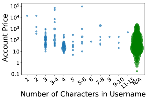
Figure 5. Price ($, log scale) of Twitter accounts with different number of characters.

We measure the economic cost for attackers to perturb the LenScreenName feature from the Twitter spam account dataset. We extract the number of characters information from 6,125 for-sale Twitter account posts, and measure the price for accounts with different username length. or unspecificed characters. In Figure 5, we plot the price of accounts according to the username length. If the post says “3 or 4 characters”, we plot the price under “3-4” category. The majority of accounts are under “N/A” category, where the sellers do not mention the length of username, but emphasize other attributes such as number of followers. Overall, if the username length has at most 4 characters, it affects the account price more than longer username.

C.2. CCSize Feature

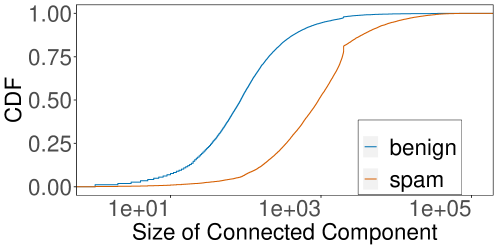
Figure 6. CDF of # of IPs in a connected component containing a given URL. Spam URLs tend to be in larger connected components.

We measure the distribution of CCSize feature from the Twitter spam URL dataset. The CCSize feature counts the number of IP nodes in the connected component of the posted URL. Since spammers reuse redirectors, their URLs often belong to the same large connected component and result in a larger CCSize feature value, compared to benign URLs, as shown in Figure 6. A larger CCSize value indicates that more resources are being reused, and the initial URL is more suspicious. Therefore, we specify CCSize feature to be monotonically increasing.

Property	Training Constraints	Robustness
Stability	Smaller $c_{\text{stability}}$	Stronger
High Confidence	Smaller $\delta$	Stronger
Redundancy	Smaller $\delta$	Stronger
Small Neighborhood	Smaller $c$ given fixed $\epsilon$	Stronger

Table 9. Robustness controlled by hyperparameters.

Stable Constant $c_{\text{stability}}$	TPR	FPR
8	0.86	0.021
4	0.835	0.031
2	0.833	0.029

Table 10. TPR and FPR of Twitter spam account classifiers trained with the stability property.

Appendix D Classification Features

Table 11 lists all the features for detecting cryptojacking, Twitter spam accounts, and Twitter spam URLs.

Dataset	Feature Name	Description	Monotonic	Low-cost
Cryptojacking	websocket	Use WebSocket APIs for network communication	Increasing
	wasm	Uses WebAssembly to execute code in browsers are near native speed	Increasing
	hash function	Use one of the hash functions on a curated list	Increasing	yes
	webworkers	The number of web workers threads for running concurrent tasks	Increasing
	messageloop load	The number of MessageLoop events for thread management	Increasing
	postmessage load	The number of PostMessage events for thread job reporting	Increasing
	parallel functions	Run the same tasks in multiple threads	Increasing
Twitter Spam Accounts	LenScreenName	The number of characters in the account user name	Increasing	yes ($\geq 5$ char)
	LenProfileDescription	The number of characters in the profile description		yes
	AgeDays	The age of the account in days	Decreasing
	NumFollowings	The number of other users an account follows	Increasing
	NumFollowers	The number of followers for an account	Decreasing
	Ratio_Following_Followers	The ratio of NumFollowings divided by NumFollowers
	StdFollowing	Standard deviation of NumFollowings over different days
	ChangeRateFollowing	The averaged difference for NumFollowings between consecutive days
	NumTweets	Total number of tweets over seven months		yes
	NumDailyTweets	Average number of daily tweets		yes
	TweetLinkRatio	Ratio of tweets containing links over total number of tweets	Increasing	yes
	TweetUniqLinkRatio	Ratio of tweets containing unique links over total number of tweets	Increasing	yes
	TweetAtRatio	Ratio of tweets containing ‘@’ over total number of tweets		yes
	TweetUniqAtRatio	Ratio of tweets with unique ‘@’ username over total number of tweets		yes
	PairwiseTweetSimilarity	Normalized avg num of common chars in pairwise tweets for a user
	Shared Resources-driven
Twitter Spam URLs	EntryURLid	In degree of the largest redirector in the connected component	Increasing
	AvgURLid	Average in degree of URL nodes in the redirection chain	Increasing
	ChainWeight	Total frequency of edges in the redirection chain	Increasing
	CCsize	Number of nodes in the connected component	Increasing
	CCdensity	Edge density of the connected component
	MinRCLen	Minimum length of the redirection chains in the connected component	Increasing
	AvgLdURLDom	Avg # of domains for landing URL IPs in the connected component	Increasing
	AvgURLDom	Average # of domains for the IPs in the redirection chain	Increasing
	Heterogeneity-driven
	GeoDist	Total geographical distance (km) traversed by the redirection chain
	CntContinent	Number of unique continents in the redirection chain
	CntCountry	Number of unique countries in the redirection chain
	CntIP	Number of unique IPs in the redirection chain
	CntDomain	Number of unique domains in the redirection chain
	CntTLD	Number of unique top-level domains in the redirection chain
	Flexibility-driven
	ChainLen	Length of the redirection chain
	EntryURLDist	Distance from the initial URL to the largest redirector
	CntInitURL	Number of initial URLs in the connected component
	CntInitURLDom	Total domain name number in the initial URLs
	CntLdURL	Number of final landing URLs in the redirection chain
	AvgIPperURL	Average IP number per URL in the connected component
	AvgIPperLdURL	Average IP number per landing URL in the connected component
	Tweet Content
	Mention Count	Number of ‘@’ that mentions other users		yes
	Hashtag Count	Number of hashtags		yes
	Tweet Count	Number of tweets made by the user account for this tweet		yes
	URL Percent	Percentage of posts from the same user that contain a URL		yes

Table 11. Classification features for three datasets. For each feature, we also mark the monotonic direction if we specify the monotonicity property, and whether we specify the feature to be low cost.

Appendix E Heuristics

The time to solve for counterexamples is the bottleneck in training. Therefore, we implement the following heuristics to improve the training efficiency:

• We exponentially increase the time out for the solver, starting from 30s. If we find at least one counterexample within each CEGIS iteration, we add the constraint(s) to eliminate the counterexample(s) and proceed with CLN training with the constraints. We increase the timeout if the solver could not find any counterexample fast enough in an iteration, and if it also could not verify that the classifier satisfies all the specified properties.

• We implement property boosting as an option to train monotonicity and stability. Property boosting means that we only train the property for the newly added sub-classifier, and keep the previous sub-classifiers fixed. This works for properties that can be satisfied if every sub-classifiers also satisfy the sub-properties, since our ensemble is a sum ensemble. If every sub-classifier is monotonic for a given feature, the ensemble classifier is also monotonic. Similarly, if every sub-classifier is stable for a given feature by a stable constant $\frac{c}{B}$, the ensemble classifier is stable under stable constant $c$.

• We use feature scheduling to train the high confidence property. Specifically, to run 10 rounds of boosting for either Twitter spam account or Twitter spam URL detection classifiers, we first boost 6 decision trees as the base model without any low-cost features. This makes sure that the base model naturally satisfies the high confidence property. Then, for the remaining 4 rounds, we use all features to boost new trees and fix the properties for the entire classifier.

• When training all the five properties (monotonicity, stability, high confidence, redundancy and small neighborhood) for the Twitter spam account detection, we use the following property scheduling to boost 6 rounds. For the first round, we use features that don’t involve any property to construct a base classifier, so it naturally satisfies all properties. In the 2nd and 3rd round, we use all features excluding low-cost ones, so we get high confidence and redundancy for free for these rounds. In the next two rounds, we use all features excluding monotonic ones, so we get monotonicity for free for these rounds. In the last round, we use all features and fix all five properties.

Property boosting, feature scheduling, and property scheduling reduce the size of the integer linear program, which makes it easier to be solved.

Appendix F Hyperparameters

Enforcing stronger robustness decreases true positive rate. The hyperparameters control this tradeoff. In particular, Table 9 shows how the strength of robustness changes as different hyperparameters change for all proposed properties except monotonicity (we don’t have such a hyperparameter for monotonicity). For example, to demonstrate the tradeoff, we trained three Twitter spam account classifiers with the stability property, where each one has a different stable constant. Table 10 shows that training with a smaller stable constant $c_{\text{stability}}$ gives us a verifiably robust model with stronger robustness but lower true positive rate.

Appendix G Obtaining More Properties

Table 8 shows that training a classifier with one property sometimes obtains another property. For the Twitter spam account detection classifiers, enforcing one of the high confidence, redundancy, and small neighborhood properties can obtain at least a second property. For example, the Logic Ensemble Redundancy model has obtained stability and high confidence properties. Since we use the same set of low-cost features to define the high confidence and redundancy properties, the redundancy property is strictly stronger than the high confidence property. In other words, if the attacker have to perturb one low-cost feature from at least two different groups to evade the classifier (redundancy), they cannot evade the classifier by perturbing only one low-cost feature (high confidence). For the largest Twitter spam URL detection dataset, the Logic Ensemble Stability model also satisfies the small neighborhood property, and the Logic Ensemble High confidence model also satisfies the stability property.

Appendix H Logic Ensemble Combined Model

Table 8 shows that, for Twitter spam account detection, the Logic Ensemble Combined with all five properties has higher AUC than the Logic Ensemble Monotonicity model trained with only one property. This is because we use property scheduling for Logic Ensemble Combined (Appendix E), such that for each round before the last round, our classifier satisfies some properties for free. We could improve the performance of the Logic Ensemble Monotonicity by similar feature scheduling technique, such as boosting first four rounds of model with non-monotonic features first, and then train with all features for later rounds.

References

- (1)
- gur ([n.d.]) [n.d.]. Gurobi Optimization. https://www.gurobi.com/.
- Albarghouthi et al. (2017) Aws Albarghouthi, Paraschos Koutris, Mayur Naik, and Calvin Smith. 2017. Constraint-based synthesis of Datalog programs. In International Conference on Principles and Practice of Constraint Programming. Springer, 689–706.
- Allix et al. (2015) Kevin Allix, Tegawendé F Bissyandé, Jacques Klein, and Yves Le Traon. 2015. Are your training datasets yet relevant?. In International Symposium on Engineering Secure Software and Systems. Springer, 51–67.
- Anil et al. (2019) Cem Anil, James Lucas, and Roger Grosse. 2019. Sorting out Lipschitz function approximation. In International Conference on Machine Learning. PMLR, 291–301.
- Archer and Wang (1993) Norman P Archer and Shouhong Wang. 1993. Application of the back propagation neural network algorithm with monotonicity constraints for two-group classification problems. Decision Sciences 24, 1 (1993), 60–75.
- Balunović et al. (2019) Mislav Balunović, Maximilian Baader, Gagandeep Singh, Timon Gehr, and Martin Vechev. 2019. Certifying geometric robustness of neural networks. Advances in Neural Information Processing Systems (NeurIPS) (2019).
- Ben-David (1995) Arie Ben-David. 1995. Monotonicity maintenance in information-theoretic machine learning algorithms. Machine Learning 19, 1 (1995), 29–43.
- Boopathy et al. (2019) Akhilan Boopathy, Tsui-Wei Weng, Pin-Yu Chen, Sijia Liu, and Luca Daniel. 2019. Cnn-cert: An efficient framework for certifying robustness of convolutional neural networks. In AAAI Conference on Artificial Intelligence (AAAI).
- Boopathy et al. (2021) Akhilan Boopathy, Tsui-Wei Weng, Sijia Liu, Pin-Yu Chen, Gaoyuan Zhang, and Luca Daniel. 2021. Fast Training of Provably Robust Neural Networks by SingleProp. AAAI Conference on Artificial Intelligence (AAAI) (2021).
- Chen and Guestrin (2016) Tianqi Chen and Carlos Guestrin. 2016. Xgboost: A scalable tree boosting system. In Proceedings of the 22nd acm sigkdd international conference on knowledge discovery and data mining. ACM, 785–794.
- Chen et al. (2020) Yizheng Chen, Shiqi Wang, Dongdong She, and Suman Jana. 2020. On Training Robust PDF Malware Classifiers. In USENIX Security Symposium.
- Cisse et al. (2017) Moustapha Cisse, Piotr Bojanowski, Edouard Grave, Yann Dauphin, and Nicolas Usunier. 2017. Parseval networks: Improving robustness to adversarial examples. In International Conference on Machine Learning. PMLR, 854–863.
- Cohen et al. (2019a) Jeremy EJ Cohen, Todd Huster, and Ra Cohen. 2019a. Universal lipschitz approximation in bounded depth neural networks. arXiv preprint arXiv:1904.04861 (2019).
- Cohen et al. (2019b) Jeremy M Cohen, Elan Rosenfeld, and J Zico Kolter. 2019b. Certified adversarial robustness via randomized smoothing. International Conference on Machine Learning (2019).
- Cropper et al. (2020) Andrew Cropper, Sebastijan Dumančić, and Stephen H Muggleton. 2020. Turning 30: New ideas in inductive logic programming. In International Joint Conferences on Artifical Intelligence (IJCAI).
- Daniels and Velikova (2010) Hennie Daniels and Marina Velikova. 2010. Monotone and partially monotone neural networks. IEEE Transactions on Neural Networks 21, 6 (2010), 906–917.
- Duivesteijn and Feelders (2008) Wouter Duivesteijn and Ad Feelders. 2008. Nearest neighbour classification with monotonicity constraints. In Joint European Conference on Machine Learning and Knowledge Discovery in Databases. Springer, 301–316.
- Dutta et al. (2018) Souradeep Dutta, Susmit Jha, Sriram Sankaranarayanan, and Ashish Tiwari. 2018. Output Range Analysis for Deep Feedforward Neural Networks. In NASA Formal Methods Symposium. Springer, 121–138.
- Dvijotham et al. (2018a) Krishnamurthy Dvijotham, Sven Gowal, Robert Stanforth, Relja Arandjelovic, Brendan O’Donoghue, Jonathan Uesato, and Pushmeet Kohli. 2018a. Training verified learners with learned verifiers. arXiv preprint arXiv:1805.10265 (2018).
- Dvijotham et al. (2018b) Krishnamurthy Dvijotham, Robert Stanforth, Sven Gowal, Timothy Mann, and Pushmeet Kohli. 2018b. A dual approach to scalable verification of deep networks. arXiv preprint arXiv:1803.06567 (2018).
- Ehlers (2017) Ruediger Ehlers. 2017. Formal Verification of Piece-Wise Linear Feed-Forward Neural Networks. 15th International Symposium on Automated Technology for Verification and Analysis (2017).
- Farnia et al. (2018) Farzan Farnia, Jesse Zhang, and David Tse. 2018. Generalizable Adversarial Training via Spectral Normalization. In International Conference on Learning Representations.
- Feelders (2010) Ad Feelders. 2010. Monotone relabeling in ordinal classification. In 2010 IEEE International Conference on Data Mining. IEEE, 803–808.
- Finlay and Oberman (2021) Chris Finlay and Adam M Oberman. 2021. Scaleable input gradient regularization for adversarial robustness. Machine Learning with Applications 3 (2021), 100017.
- Fischer et al. (2019) Marc Fischer, Mislav Balunovic, Dana Drachsler-Cohen, Timon Gehr, Ce Zhang, and Martin Vechev. 2019. DL2: Training and Querying Neural Networks with Logic. In International Conference on Machine Learning (ICML).
- Fischetti and Jo (2017) Matteo Fischetti and Jason Jo. 2017. Deep Neural Networks as 0-1 Mixed Integer Linear Programs: A Feasibility Study. arXiv preprint arXiv:1712.06174 (2017).
- Friedman et al. (2008) Jerome H Friedman, Bogdan E Popescu, et al. 2008. Predictive learning via rule ensembles. The Annals of Applied Statistics 2, 3 (2008), 916–954.
- Gehr et al. (2018) Timon Gehr, Matthew Mirman, Dana Drachsler-Cohen, Petar Tsankov, Swarat Chaudhuri, and Martin Vechev. 2018. Ai 2: Safety and robustness certification of neural networks with abstract interpretation. In IEEE Symposium on Security and Privacy (SP).
- Goncharov ([n.d.]) Maxim Goncharov. [n.d.]. Traffic direction systems as malware distribution tools. http://www.trendmicro.es/media/misc/malware-distribution-tools-research-paper-en.pdf.
- Gouk et al. (2021) Henry Gouk, Eibe Frank, Bernhard Pfahringer, and Michael J Cree. 2021. Regularisation of neural networks by enforcing lipschitz continuity. Machine Learning 110, 2 (2021), 393–416.
- Grosse et al. (2016) Kathrin Grosse, Nicolas Papernot, Praveen Manoharan, Michael Backes, and Patrick McDaniel. 2016. Adversarial perturbations against deep neural networks for malware classification. arXiv preprint arXiv:1606.04435 (2016).
- Gupta et al. (2016) Maya Gupta, Andrew Cotter, Jan Pfeifer, Konstantin Voevodski, Kevin Canini, Alexander Mangylov, Wojciech Moczydlowski, and Alexander Van Esbroeck. 2016. Monotonic calibrated interpolated look-up tables. The Journal of Machine Learning Research 17, 1 (2016), 3790–3836.
- Hein and Andriushchenko (2017) Matthias Hein and Maksym Andriushchenko. 2017. Formal guarantees on the robustness of a classifier against adversarial manipulation. In Advances in Neural Information Processing Systems.
- Huang et al. (2017) Xiaowei Huang, Marta Kwiatkowska, Sen Wang, and Min Wu. 2017. Safety verification of deep neural networks. In International Conference on Computer Aided Verification (CAV). Springer, 3–29.
- Incer et al. (2018) Inigo Incer, Michael Theodorides, Sadia Afroz, and David Wagner. 2018. Adversarially Robust Malware Detection Using Monotonic Classification. In Proceedings of the Fourth ACM International Workshop on Security and Privacy Analytics. ACM, 54–63.
- Jia et al. (2019) Jinyuan Jia, Xiaoyu Cao, Binghui Wang, and Neil Zhenqiang Gong. 2019. Certified robustness for top-k predictions against adversarial perturbations via randomized smoothing. International Conference on Learning Representations (ICLR) (2019).
- Kantchelian et al. (2016) Alex Kantchelian, JD Tygar, and Anthony Joseph. 2016. Evasion and hardening of tree ensemble classifiers. In International Conference on Machine Learning. 2387–2396.
- Katz et al. (2017) Guy Katz, Clark Barrett, David L Dill, Kyle Julian, and Mykel J Kochenderfer. 2017. Reluplex: An efficient SMT solver for verifying deep neural networks. In International Conference on Computer Aided Verification (CAV). Springer, 97–117.
- Katz et al. (2019) Guy Katz, Derek A Huang, Duligur Ibeling, Kyle Julian, Christopher Lazarus, Rachel Lim, Parth Shah, Shantanu Thakoor, Haoze Wu, Aleksandar Zeljić, et al. 2019. The marabou framework for verification and analysis of deep neural networks. In International Conference on Computer Aided Verification (CAV).
- Kay and Ungar (2000) Herbert Kay and Lyle H Ungar. 2000. Estimating monotonic functions and their bounds. AIChE Journal 46, 12 (2000), 2426–2434.
- Kharraz et al. (2019) Amin Kharraz, Zane Ma, Paul Murley, Charles Lever, Joshua Mason, Andrew Miller, Nikita Borisov, Manos Antonakakis, and Michael Bailey. 2019. Outguard: Detecting in-browser covert cryptocurrency mining in the wild. In The World Wide Web Conference. 840–852.
- Kurakin et al. (2017) Alexey Kurakin, Ian Goodfellow, and Samy Bengio. 2017. Adversarial machine learning at scale. In International Conference on Learning Representations (ICLR).
- Kwon et al. (2017) Heeyoung Kwon, Mirza Basim Baig, and Leman Akoglu. 2017. A domain-agnostic approach to spam-URL detection via redirects. In Pacific-Asia Conference on Knowledge Discovery and Data Mining. Springer, 220–232.
- Laskov et al. (2014) Pavel Laskov et al. 2014. Practical evasion of a learning-based classifier: A case study. In Security and Privacy (SP), 2014 IEEE Symposium on. IEEE, 197–211.
- Lecuyer et al. (2019) Mathias Lecuyer, Vaggelis Atlidakis, Roxana Geambasu, Daniel Hsu, and Suman Jana. 2019. Certified robustness to adversarial examples with differential privacy. In 2019 IEEE Symposium on Security and Privacy (SP). IEEE.
- Lee et al. (2010) Kyumin Lee, James Caverlee, and Steve Webb. 2010. Uncovering social spammers: social honeypots+ machine learning. In Proceedings of the 33rd international ACM SIGIR conference on Research and development in information retrieval. 435–442.
- Lee et al. (2011) Kyumin Lee, Brian Eoff, and James Caverlee. 2011. Seven months with the devils: A long-term study of content polluters on twitter. In Proceedings of the International AAAI Conference on Web and Social Media, Vol. 5.
- Lee and Kim (2013) Sangho Lee and Jong Kim. 2013. Warningbird: A near real-time detection system for suspicious urls in twitter stream. IEEE transactions on dependable and secure computing 10, 3 (2013), 183–195.
- Lee et al. (2020) Sungyoon Lee, Jaewook Lee, and Saerom Park. 2020. Lipschitz-Certifiable Training with a Tight Outer Bound. Advances in Neural Information Processing Systems (NeurIPS) (2020).
- Leino et al. (2021) Klas Leino, Zifan Wang, and Matt Fredrikson. 2021. Globally-Robust Neural Networks. arXiv preprint arXiv:2102.08452 (2021).
- Li et al. (2018) Bai Li, Changyou Chen, Wenlin Wang, and Lawrence Carin. 2018. Second-order adversarial attack and certifiable robustness. (2018).
- Li et al. (2019a) Bai Li, Changyou Chen, Wenlin Wang, and Lawrence Carin. 2019a. Certified adversarial robustness with additive noise. Advances in Neural Information Processing Systems (NeurIPS) (2019).
- Li et al. (2020) Linyi Li, Xiangyu Qi, Tao Xie, and Bo Li. 2020. SoK: Certified Robustness for Deep Neural Networks. arXiv preprint arXiv:2009.04131 (2020).
- Li et al. (2019b) Linyi Li, Zexuan Zhong, Bo Li, and Tao Xie. 2019b. Robustra: Training Provable Robust Neural Networks over Reference Adversarial Space. In IJCAI.
- Li et al. (2013) Zhou Li, Sumayah Alrwais, Yinglian Xie, Fang Yu, and XiaoFeng Wang. 2013. Finding the linchpins of the dark web: a study on topologically dedicated hosts on malicious web infrastructures. In 2013 IEEE Symposium on Security and Privacy. IEEE, 112–126.
- Lin et al. (2020) Xuankang Lin, He Zhu, Roopsha Samanta, and Suresh Jagannathan. 2020. ART: abstraction refinement-guided training for provably correct neural networks. In 2020 Formal Methods in Computer Aided Design (FMCAD). IEEE, 148–157.
- Lomuscio and Maganti (2017) Alessio Lomuscio and Lalit Maganti. 2017. An approach to reachability analysis for feed-forward relu neural networks. arXiv preprint arXiv:1706.07351 (2017).
- Ma et al. (2009) Justin Ma, Lawrence K Saul, Stefan Savage, and Geoffrey M Voelker. 2009. Identifying suspicious URLs: an application of large-scale online learning. In Proceedings of the 26th annual international conference on machine learning. 681–688.
- Madry et al. (2018) Aleksander Madry, Aleksandar Makelov, Ludwig Schmidt, Dimitris Tsipras, and Adrian Vladu. 2018. Towards deep learning models resistant to adversarial attacks. International Conference on Learning Representations (ICLR) (2018).
- Melacci et al. (2020) Stefano Melacci, Gabriele Ciravegna, Angelo Sotgiu, Ambra Demontis, Battista Biggio, Marco Gori, and Fabio Roli. 2020. Can Domain Knowledge Alleviate Adversarial Attacks in Multi-Label Classifiers? arXiv preprint arXiv:2006.03833 (2020).
- Miller et al. (2016) Brad Miller, Alex Kantchelian, Michael Carl Tschantz, Sadia Afroz, Rekha Bachwani, Riyaz Faizullabhoy, Ling Huang, Vaishaal Shankar, Tony Wu, George Yiu, et al. 2016. Reviewer integration and performance measurement for malware detection. In International Conference on Detection of Intrusions and Malware, and Vulnerability Assessment. Springer, 122–141.
- Mirman et al. (2018) Matthew Mirman, Timon Gehr, and Martin Vechev. 2018. Differentiable Abstract Interpretation for Provably Robust Neural Networks. In International Conference on Machine Learning (ICML). 3575–3583.
- Müller et al. (2021b) Christoph Müller, François Serre, Gagandeep Singh, Markus Püschel, and Martin Vechev. 2021b. Scaling Polyhedral Neural Network Verification on GPUs. Proceedings of Machine Learning and Systems 3 (2021).
- Müller et al. (2021a) Mark Niklas Müller, Gleb Makarchuk, Gagandeep Singh, Markus Püschel, and Martin Vechev. 2021a. Precise Multi-Neuron Abstractions for Neural Network Certification. arXiv preprint arXiv:2103.03638 (2021).
- Pauli et al. (2021) Patricia Pauli, Anne Koch, Julian Berberich, Paul Kohler, and Frank Allgower. 2021. Training robust neural networks using Lipschitz bounds. IEEE Control Systems Letters (2021).
- Pendlebury et al. (2019) Feargus Pendlebury, Fabio Pierazzi, Roberto Jordaney, Johannes Kinder, and Lorenzo Cavallaro. 2019. TESSERACT: Eliminating experimental bias in malware classification across space and time. In 28th USENIX Security Symposium (USENIX Security 19). 729–746.
- Pierazzi et al. (2020) F. Pierazzi, F. Pendlebury, J. Cortellazzi, and L. Cavallaro. 2020. Intriguing Properties of Adversarial ML Attacks in the Problem Space. In 2020 IEEE Symposium on Security and Privacy (SP). IEEE Computer Society, 1308–1325. https://doi.org/10.1109/SP40000.2020.00073
- Qin et al. (2019) Chongli Qin, James Martens, Sven Gowal, Dilip Krishnan, Krishnamurthy Dvijotham, Alhussein Fawzi, Soham De, Robert Stanforth, and Pushmeet Kohli. 2019. Adversarial robustness through local linearization. Advances in Neural Information Processing Systems (NIPS) (2019).
- Raghothaman et al. (2019) Mukund Raghothaman, Jonathan Mendelson, David Zhao, Mayur Naik, and Bernhard Scholz. 2019. Provenance-guided synthesis of Datalog programs. Proceedings of the ACM on Programming Languages 4, POPL (2019), 1–27.
- Raghunathan et al. (2018a) Aditi Raghunathan, Jacob Steinhardt, and Percy Liang. 2018a. Certified defenses against adversarial examples. International Conference on Learning Representations (ICLR) (2018).
- Raghunathan et al. (2018b) Aditi Raghunathan, Jacob Steinhardt, and Percy S Liang. 2018b. Semidefinite relaxations for certifying robustness to adversarial examples. In Advances in Neural Information Processing Systems. 10900–10910.
- Ryan et al. (2020) Gabriel Ryan, Justin Wong, Jianan Yao, Ronghui Gu, and Suman Jana. 2020. CLN2INV: Learning Loop Invariants with Continuous Logic Networks. In International Conference on Learning Representations (ICLR).
- Salman et al. (2019a) Hadi Salman, Greg Yang, Jerry Li, Pengchuan Zhang, Huan Zhang, Ilya Razenshteyn, and Sebastien Bubeck. 2019a. Provably robust deep learning via adversarially trained smoothed classifiers. Advances in Neural Information Processing Systems (NeurIPS) (2019).
- Salman et al. (2019b) Hadi Salman, Greg Yang, Huan Zhang, Cho-Jui Hsieh, and Pengchuan Zhang. 2019b. A convex relaxation barrier to tight robustness verification of neural networks. Advances in Neural Information Processing Systems (NeurIPS) (2019).
- Si et al. (2018) Xujie Si, Woosuk Lee, Richard Zhang, Aws Albarghouthi, Paraschos Koutris, and Mayur Naik. 2018. Syntax-guided synthesis of datalog programs. In Proceedings of the 2018 26th ACM Joint Meeting on European Software Engineering Conference and Symposium on the Foundations of Software Engineering. 515–527.
- Singh et al. (2019a) Gagandeep Singh, Rupanshu Ganvir, Markus Püschel, and Martin Vechev. 2019a. Beyond the single neuron convex barrier for neural network certification. Advances in Neural Information Processing Systems (NeurIPS) (2019).
- Singh et al. (2019b) Gagandeep Singh, Timon Gehr, Markus Püschel, and Martin Vechev. 2019b. An abstract domain for certifying neural networks. Proceedings of the ACM on Programming Languages 3, POPL (2019), 1–30.
- Singh et al. (2019c) Gagandeep Singh, Timon Gehr, Markus Püschel, and Martin T Vechev. 2019c. Boosting Robustness Certification of Neural Networks.. In ICLR (Poster).
- Singla and Feizi (2019) Sahil Singla and Soheil Feizi. 2019. Bounding singular values of convolution layers. arXiv preprint arXiv:1911.10258 (2019).
- Solar-Lezama et al. (2006) Armando Solar-Lezama, Liviu Tancau, Rastislav Bodik, Sanjit Seshia, and Vijay Saraswat. 2006. Combinatorial sketching for finite programs. In Proceedings of the 12th international conference on Architectural support for programming languages and operating systems. 404–415.
- Szegedy et al. (2013) Christian Szegedy, Wojciech Zaremba, Ilya Sutskever, Joan Bruna, Dumitru Erhan, Ian Goodfellow, and Rob Fergus. 2013. Intriguing properties of neural networks. International Conference on Learning Representations (ICLR) (2013).
- Thomas et al. (2011) Kurt Thomas, Chris Grier, Justin Ma, Vern Paxson, and Dawn Song. 2011. Design and evaluation of a real-time url spam filtering service. In 2011 IEEE symposium on security and privacy. IEEE, 447–462.
- Tjeng et al. (2017) Vincent Tjeng, Kai Xiao, and Russ Tedrake. 2017. Evaluating Robustness of Neural Networks with Mixed Integer Programming. arXiv preprint arXiv:1711.07356 (2017).
- Wagner and Soto (2002) David Wagner and Paolo Soto. 2002. Mimicry attacks on host-based intrusion detection systems. In Proceedings of the 9th ACM Conference on Computer and Communications Security. ACM, 255–264.
- Wang et al. (2018a) Shiqi Wang, Yizheng Chen, Ahmed Abdou, and Suman Jana. 2018a. MixTrain: Scalable Training of Formally Robust Neural Networks. arXiv preprint arXiv:1811.02625 (2018).
- Wang et al. (2018b) Shiqi Wang, Kexin Pei, Whitehouse Justin, Junfeng Yang, and Suman Jana. 2018b. Efficient Formal Safety Analysis of Neural Networks. Advances in Neural Information Processing Systems (NIPS) (2018).
- Wang et al. (2018c) Shiqi Wang, Kexin Pei, Whitehouse Justin, Junfeng Yang, and Suman Jana. 2018c. Formal Security Analysis of Neural Networks using Symbolic Intervals. 27th USENIX Security Symposium (2018).
- Wang et al. (2021) Shiqi Wang, Huan Zhang, Kaidi Xu, Xue Lin, Suman Jana, Cho-Jui Hsieh, and J Zico Kolter. 2021. Beta-CROWN: Efficient Bound Propagation with Per-neuron Split Constraints for Complete and Incomplete Neural Network Verification. arXiv preprint arXiv:2103.06624 (2021).
- Wehenkel and Louppe (2019) Antoine Wehenkel and Gilles Louppe. 2019. Unconstrained monotonic neural networks. In Advances in Neural Information Processing Systems.
- Weng et al. (2018a) Lily Weng, Huan Zhang, Hongge Chen, Zhao Song, Cho-Jui Hsieh, Luca Daniel, Duane Boning, and Inderjit Dhillon. 2018a. Towards fast computation of certified robustness for relu networks. In International Conference on Machine Learning (ICML).
- Weng et al. (2018b) Tsui-Wei Weng, Huan Zhang, Pin-Yu Chen, Jinfeng Yi, Dong Su, Yupeng Gao, Cho-Jui Hsieh, and Luca Daniel. 2018b. Evaluating the robustness of neural networks: An extreme value theory approach. In International Conference on Learning Representations (ICLR).
- Wong and Kolter (2018) Eric Wong and Zico Kolter. 2018. Provable defenses against adversarial examples via the convex outer adversarial polytope. In International Conference on Machine Learning. 5283–5292.
- Wong et al. (2018) Eric Wong, Frank Schmidt, Jan Hendrik Metzen, and J Zico Kolter. 2018. Scaling provable adversarial defenses. Advances in Neural Information Processing Systems (NIPS) (2018).
- Xu et al. (2021) Kaidi Xu, Huan Zhang, Shiqi Wang, Yihan Wang, Suman Jana, Xue Lin, and Cho-Jui Hsieh. 2021. Fast and complete: Enabling complete neural network verification with rapid and massively parallel incomplete verifiers. International Conference on Learning Representations (ICLR) (2021).
- Yang et al. (2020) Greg Yang, Tony Duan, J Edward Hu, Hadi Salman, Ilya Razenshteyn, and Jerry Li. 2020. Randomized smoothing of all shapes and sizes. In International Conference on Machine Learning (ICML). PMLR.
- Yao et al. (2020) Jianan Yao, Gabriel Ryan, Justin Wong, Suman Jana, and Ronghui Gu. 2020. Learning Nonlinear Loop Invariants with Gated Continuous Logic Networks. In Proceedings of the 41st ACM SIGPLAN Conference on Programming Language Design and Implementation.
- Zhang et al. (2020) Huan Zhang, Hongge Chen, Chaowei Xiao, Sven Gowal, Robert Stanforth, Bo Li, Duane Boning, and Cho-Jui Hsieh. 2020. Towards stable and efficient training of verifiably robust neural networks. International Conference on Learning Representations (ICLR) (2020).
- Zhang et al. (2018) Huan Zhang, Tsui-Wei Weng, Pin-Yu Chen, Cho-Jui Hsieh, and Luca Daniel. 2018. Efficient neural network robustness certification with general activation functions. arXiv preprint arXiv:1811.00866 (2018).
- Zhang and Evans (2019) Xiao Zhang and David Evans. 2019. Cost-Sensitive Robustness against Adversarial Examples. International Conference on Learning Representations (ICLR) (2019).