Reconstructing Small 3D Objects in front of a Textured Background

Abstract

We present a technique for a complete 3D reconstruction of small objects moving in front of a textured background. It is a particular variation of multibody structure from motion, which specializes to two objects only. The scene is captured in several static configurations between which the relative pose of the two objects may change. We reconstruct every static configuration individually and segment the points locally by finding multiple poses of cameras that capture the scene’s other configurations. Then, the local segmentation results are combined, and the reconstructions are merged into the resulting model of the scene. In experiments with real artifacts, we show that our approach has practical advantages when reconstructing 3D objects from all sides. In this setting, our method outperforms the state-of-the-art. We integrate our method into the state of the art 3D reconstruction pipeline COLMAP.

1 Introduction

Structure-from-Motion (SfM) [49] is an important problem of estimating the 3D model of a scene from two-dimensional images of the scene [51, 52, 49, 13, 31], image matching [43, 11], visual odometry [37, 1] and visual localization [47, 54, 55].

In the digitization of cultural heritage [9], movie [5] and game [17] industries, it is crucial to reconstruct complete models of small objects. Often, this is done by running an SfM pipeline on images of small objects presented from all sides on a featureless background [39]. Small objects, however, often have repetitive structures and are close to planar in some views. Hence, they do not provide reliable camera poses, which leads to low quality 3D reconstructions. This can be remedied by capturing a structured background together with the object, Fig. 1. Then, however, segmentation is needed to reconstruct the moving object in front of the background. To this end, we develop the TBSfM method, a particular variation of two-body SfM for high-quality complete 3D reconstruction of objects moving in front of a textured background.

SfM is well understood for static scenes with a single rigid object and has many practical applications in, e.g., cartography [10], archaeology [68], and film industry [4]. In the case of dynamic scenes, the majority of works [15, 57, 41, 48, 38, 44] and [14, 45, 24, 23, 66, 16] assume video input, while the case of unordered input images has not been fully explored yet. To our best knowledge, there is no full Multi-Body SfM (MBSfM) pipeline producing satisfactory results in industrial quality. Existing partial results [41, 38, 48, 53] indicate that the multi-body segmentation in SfM is a difficult task. Hence, we address a specialized version of an MBSfM problem by restricting ourselves to two objects and to a semidynamic acquisition of the images of the scene. Although the setting is more restrictive when compared to the general MBSfM, the problem is still challenging and has practical use.

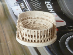
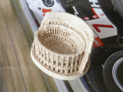
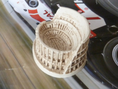
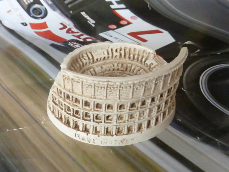
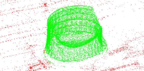
Figure 1: (left) Multiple images of an artefact moving in front of a textured background. (right) Reconstructed 3D model capturing the artefact from all sides (green) together with the reconstructed background (red). Our TBSfM segments artifacts from the background and delivers 3D reconstruction of both rigid bodies. Background helps to obtain more 3D points artefacts and reduces reprojection errors, see Tab. 1.

We consider unordered and unstructured input images, which is a typical setup for SfM 3D reconstruction. Therefore, the works which assume video input, for example [15, 57, 41, 48, 38, 44, 14, 45, 24, 23, 66, 16], cannot solve our problem. We also assume that the images may capture the scene from different viewpoints and most of the points are observed only by a small portion of cameras. The MBSfM works based on factorization, e.g., [62, 72, 64, 42, 30, 12, 27, 20, 8, 28, 46, 22], use a track completion, as the factorization itself requires complete tracks. However, in our setting, the track completion is an underconstrained problem, as [6] proves the existence of a lower bound on the number of samples present in a matrix, below which no algorithm can guarantee a successful matrix completion. (Sec. 4.2) Other MBSfM works, e.g. [29, 26, 71], evaluate the distances between each pair of points and therefore are not suitable for large scenes with more than tens of thousands of points because the distances are unable to fit into computer memory. We assume arbitrarily large scenes, therefore, these methods are not suitable for our setting too.

1.1 Contribution

We present Two-Body Structure from Motion for Semidynamic Scenes, a generalization of SfM to two independently moving objects in the scene, assuming that the scene is captured in several static configurations between which the relative pose of the two objects may change. Our TBSfM reconstructs every static configuration individually and segments the points locally by finding multiple poses of cameras which capture the other configurations of the scene. We demonstrate that TBSfM has a practical use in the reconstruction of small artifacts and that it outperforms the state-of-the-art. It is able to improve the quality of the reconstruction of small and repetitive objects when placed on a textured background. Most of the existing MBSfM pipelines reconstruct each object individually, and therefore, they are not able to resolve the problem of scale consistency. To overcome this problem, we reconstruct the foreground object together with the background and segment points afterwards, which is possible thanks to the semidynamic setting. Then, the scale of the foreground model is consistent with the scale of the background model.

Our method has two significant advantages when compared to the general approach to MBSfM, which is to first segment tracks and then reconstruct each object individually. First, we evade the segmentation of the 2D tracks, which is a difficult task which might be degenerated [18]. Secondly, the experiments show that the presence of the background in the reconstruction step may significantly improve the result. (See Section 4.3)

1.2 Related work

General MBSfM is closely related to Motion segmentation (MS), which clusters points into different motions. Two view MS can be achieved with multiple model fitting. MS methods use consensus analysis [70, 65, 75, 35], preference analysis [74, 58, 7, 32, 40, 34], energy minimization [19, 3], branch and bound [56], subspace segmentation [63], or information theory [60]. Three-view MS is described in [64]. Some multiview MS methods use subspace segmentation [62, 72, 64, 42, 30, 12, 27, 20]. The subspace segmentation requires complete tracks. Therefore, these methods demand a completion of the tracks to pass from incomplete tracks to the complete ones. The completion of tracks works only when a small number of observations are missing. In our case, the points are observed by a few cameras and, therefore, the track completion is an underconstrained problem. Other methods combine results from two view methods [29, 26, 71, 2]. Except for [2], these methods evaluate the distances between each pair of points and, therefore, are not suitable for large scenes due to their spatial complexity. Work [25] assumes that the motion is known a priory and detects the moving objects as points inconsistent with the motion. The goal of MBSfM is to segment moving objects in the scene and to provide their 3D reconstruction. Works [15, 57, 41, 48, 38, 44, 14] and [45, 24, 23, 66, 16] require video sequences as the input. Work [15] introduces a constraint on internal parameters and segments points together with building the tracks. In [57], the initial segmentation is found and propagated throughout the video sequence. In [41] a matrix indicating the similarity between two points is found and decomposed with SVD. [48] builds tentative motions and selects the most relevant ones with an information criterion. In [38], 3D reconstruction and motion segmentation are performed simultaneously. The work handles incomplete tracks and changing number of motions. In [44], the structure, motion and segmentation are found simultaneously with energy minimization and the output is a dense reconstruction. Work [24] performs SfM with additional feedback from motion segmentation and from a particle filter. Work [14] handles articulated motions. Non-rigid motions are addressed in [45, 23, 66, 16]. Works [8, 28, 46, 22] use subspace clustering. All the above methods require complete tracks. While [8] assumes affine projection, [28, 46] handle perspective projection. [22] handles multiple nonrigid motions. Work [73] requires the motion segmentation as its input, it outputs a corrected segmentation together with the 3D model.

The most relevant previous work is YASFM [53]. Unlike the majority of the methods, [53] handles unordered input images and does not require complete tracks. In [53], the planes are segmented with growing homographies and grouped together if they belong to the same motion according to a planar homology score. Unfortunately, due to the greedy nature of the grouping algorithm, [53] typically fails if there is no motion between some images. Our work is an extension of COLMAP SfM pipeline [49], which already contains some elements used in MBSfM. For instance, it can verify matches from different objects. However, [49] does not deal with dynamic scenes with multiple objects.

2 Problem formulation

We will now formulate TBSfM problem. We use the nomenclature from [18], $\pi$ denotes the calibrated perspective projection, i.e., $\pi([x,y,z])=[x/z,y/z]$. $[1,n]$ is an abbreviation of $1,...,n$.

The scene we wish to reconstruct consists of two objects; the background and the foreground. The scene contains $n$ points and is captured in $k$ different static configurations by image sequences called takes. The background remains static, while the foreground moves between the takes.

Let $i\in[1,n]$ denote a point id. We introduce point-labeling function $o(i)\in\{B,F,U\}$, which assigns points to the foreground (F), background (B), and marks as unknown (U) points that were not assigned to F or B, e.g. due to mismatches. Then, $X_{i,\delta}^{o(i)}\in\mathbb{R}^{3}$ denotes the $i^{th}$ point in the initial configuration and in the world coordinate system $\delta$.

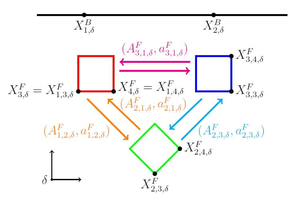
(a)

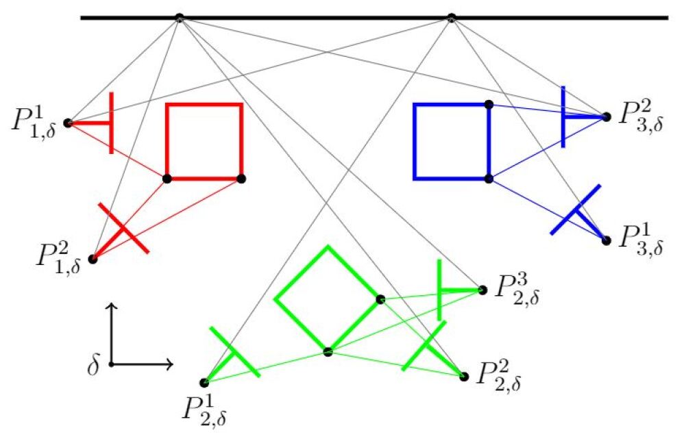
(b)

Figure 2: Example of a scene with $k=3$ takes and $m=4$ points. The red, green and blue boxes represent three different positions of the object. The black line represents the background. (a) The arrows represent the motions between those. (b) The scene is observed with 7 cameras. Every take is observed by the cameras of the corresponding color.

2.1 Motion between the takes

We will now describe how the points move between different configurations.

The points appear in different positions according to take $t\in[1,k]$, in which they are captured. Let $X_{t,i,\delta}^{o(i)}\in\mathbb{R}^{3}$ be the position of point $i$ in take $t$ and in the world coordinate system $\delta$. Let $(A_{t,\delta}^{o},a_{t,\delta}^{o})$, with rotation $A_{t,\delta}^{o}$ and translation $a_{t,\delta}^{o}$, denote the motion of object $o\in\{B,F\}$ from the initial configuration to take $t$. Then we have

$$X_{t,i,\delta}^{o(i)}=A_{t,\delta}^{o(i)}X_{i,\delta}^{o(i)}+a_{t,\delta}^{o(i)}$$ (1)

The background remains static and the initial position is equal to take $1$, therefore if $o=B$ or $t=1$, we can write

$$A_{t,\delta}^{o}=I;a_{t,\delta}^{o}=0$$ (2)

Let $(A_{s,t,\delta}^{o},a_{s,t,\delta}^{o})$ denote the motion of object $o$ from take $s$ to take $t$. This motion is composed of the motions between the takes and the initial position as

$$A_{s,t,\delta}^{o}=A_{t,\delta}^{o}(A_{s,\delta}^{o})^{-1};\ a_{s,t,\delta}^{o}=a_{t,\delta}^{o(i)}-A_{t,\delta}^{o(i)}(A_{s,\delta}^{o(i)})^{-1}a_{s,\delta}^{o(i)}$$ (3)

A scene with the motions is illustrated in Fig. 2(a).

2.2 Cameras observing the configurations

Next, we explain how the configurations of the scene are observed by cameras.

Every take $t\in[1,k]$ is captured by $m_{t}\geq 2$ cameras. We assume the perspective camera model [18]. Let $m=\sum_{t=1}^{k}~{}m_{t}$ be the total number of cameras. Let $j~{}\in~{}[1,m]$ be the id of a camera. Let $t(j)$ be the take observed by the camera $j$. Let $P_{\delta}^{j}=K^{j}\begin{bmatrix}R_{\delta}^{j}\ |-R_{\delta}^{j}c_{\delta}^{j}\end{bmatrix}$ denote the camera matrix and $x_{t(j),i}^{j}$ denote the projection of point $X_{t(j),i,\delta}^{o(i)}$ into camera $P_{\delta}^{j}$. The point is projected as

$$\alpha x_{t(j),i}^{j} = K^{j}R_{\delta}^{j}(X_{t(j),i,\delta}^{o(i)}-c_{\delta}^{j});\ \alpha\in\mathbb{R}$$ (4)

$$\alpha x_{t(j),i}^{j} = K^{j}R_{\delta}^{j}(A_{t(j),\delta}^{o(i)}X_{i,\delta}^{o(i)}+a_{t(j),\delta}^{o(i)}-c_{\delta}^{j})$$ (5)

The cameras observing the scene are illustrated in Fig. 2(b).

2.3 The two-body SfM task

We will now formulate our main task.

First, we define the reprojection error of the observation $x_{t(j),i}^{j}$ as follows. For point labels $o(i)\in\{B,F\}$, we set

$$e_{t(j),i}^{j}=\lVert\pi(x_{t(j),i}^{j})-\pi(R_{\delta}^{j}(A_{t(j),\delta}^{o(i)}X_{t(j),i,\delta}^{o(i)}+a_{t(j),\delta}^{o(i)}-c_{\delta}^{j})\lVert$$

For $o(i)\in\{U\}$, we set it to a constant value $\epsilon$, i.e.,  $e_{t,i}^{j_{t}}=\epsilon$.

Then, introducing points $\theta_{1}=\{X_{i,\delta}^{o(i)};i=[1,n]\}$, foreground motions $\theta_{2}=\{(A_{t,\delta}^{F},a_{t,\delta}^{F});t=[2,k]\}$, and camera projections $\theta_{3}=\{P_{\delta}^{j};,j=[1,m]\}$, the scene can be described with parameters $\theta=\{o(i),\theta_{1},\theta_{2},\theta_{3}\}$.

The TBSfM task is to

1) Segment the scene into two objects, F and B, and points with label U by finding the optimal labeling

$$o(i)^{*}=\underset{\theta}{\operatorname{argmax}}\#(e_{t(j),i}^{j}<\epsilon)$$ (6)

with $o(i)^{*}=U$ when $e_{t(j),i}^{j}\geq\epsilon$.

2) Reconstruct the two objects in the initial position from input observations $x_{t(j),i}^{j}$ by finding optimal parameters $\phi=\{\theta_{1},\theta_{2},\theta_{3}\}$

$$\phi^{*}=\underset{\phi}{\operatorname{argmin}}\sum_{i,j,t(j)}(e_{t(j),i}^{j})^{2}$$ (7)

The value of the function (7) does not depend on the points labeled by U because their reprojection error is set to the constant $\epsilon$.

3 Proposed TBSfM method

TBSfM task is known to be hard and its exact solution is not feasible [36]. We thus propose a greedy approximate solution and show that it achieves good results in practice.

Our method, which is concisely presented in Alg. 1, starts with reconstructing static configurations with a state-of-the-art pipeline [49]. Then, it finds the poses of the cameras from other takes towards the background and towards the foreground. Inliers of these poses give local segmentations. Then, the poses are grouped to obtain the global segmentation to merge partial reconstructions of the static configurations into the resulting model.

input : Images of the scene in different takes

output : Model of the scene with point labelling $o(i)$

for take $t\in[1,k]$ do

       (Sec. 3.1) Reconstruct model of take $t$;

       (Sec. 3.2) Sequentially register cameras from other takes $s,s\neq t$ towards $t$;

       (Sec. 3.3) Merge the observations of the sequentially registered cameras;

      

end for

Sec. 3.5 Merge the groups of points from different takes;

(Sec. 3.6) Merge the models according to [21];

Perform Bundle Adjustment [61] where function (7) is minimized;

Algorithm 1 Two Body SfM.

We will next describe the individual elements of the TBSfM algorithm.

3.1 Reconstruction of the takes

The input of the method is a set of images grouped into takes. The first step is to reconstruct every take separately by COLMAP SfM pipeline [49]. The output is a set of $k$ models with matches between the corresponding 3D points.

The models reconstructed separately from the takes are in their own coordinate systems $\delta_{t}$, $t\in[1,k]$. Let $X_{t,i,\delta_{t}}^{o(i)}$ be the position of point $X_{t,i,\delta}^{o(i)}$ in coordinate system $\delta_{t}$. Let $(B_{t},b_{t},\beta_{t})$, $B_{t}\in SO(3),b_{t}\in\mathbb{R}^{3},\beta_{t}\in\mathbb{R}^{+}$ denote the change of coordinates between systems $\delta$ and $\delta_{t}$. Then,

$$X_{t,i,\delta_{t}}^{o(i)}=\beta_{t}B_{t}X_{t,i,\delta}^{o(i)}+b_{t}$$ (8)

The change of coordinates $(B_{s,t},b_{s,t},\beta_{s,t})$ between systems $\delta_{s}$, $\delta_{t}$ is composed from the changes of coordinates between the systems and the world coordinate system $\delta$ as

$$B_{s,t}=B_{t}B_{s}^{-1};\ b_{s,t}=b_{t}-\frac{\beta_{t}}{\beta_{s}}B_{t}B_{s}^{-1}b_{s};\ \beta_{s,t}=\frac{\beta_{t}}{\beta_{s}}$$ (9)

Let $P_{t,\delta_{t}}^{j_{t}}$ denote camera $P_{t,\delta}^{j_{t}}$ in system $\delta_{t}$, and $(A_{s,t,\delta_{t}}^{o},a_{s,t,\delta_{t}}^{o})$ denote the motion $(A_{s,t,\delta}^{o},a_{s,t,\delta}^{o})$ of object $o$ in coordinate system $\delta_{t}$.

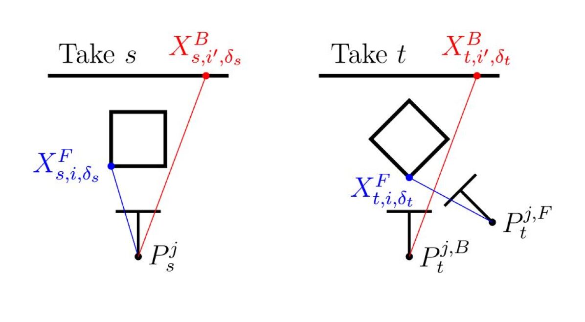
(a)

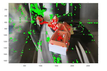
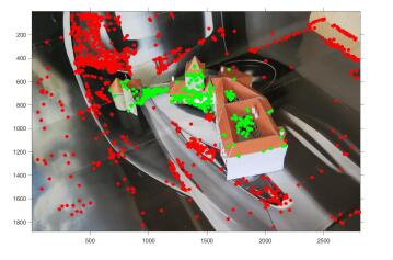
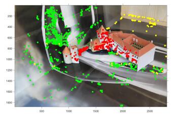
(b)

Figure 3: (a) Illustration of two poses of a camera from take $s$ towards take $t$. The figure shows that a camera has two different poses towards a different take; one towards the background and one towards the foreground. (b) Different results of the sequential PnP. Three cameras from take $s$ which were registered towards take $t$. Inliers to the first pose are green, inliers to the second pose are red, inliers to the third pose are yellow.

3.2 Registration of cameras from other takes

The next task is to find the segmentation of the points and to combine the $k$ models into one. We will first show how the poses of the cameras from other takes can be used to label the points.

The key observation is that camera $P_{s}^{j}$ from take $s$ has two different poses towards take $t\neq s$; one towards the background and one towards the foreground, as shown in Fig. 3(a). Let us denote by $P_{t}^{j,B}$ the pose towards the background and by $P_{t}^{j,F}$ the pose towards the foreground.

Then, the projection of point $X_{t,i,\delta_{t}}^{F}$ from the foreground onto camera $P_{t}^{j,F}$ is the same as the projection of point $X_{s,i,\delta_{s}}^{F}$ onto camera $P_{s}^{j}$. So, the reprojection error of points from foreground on camera $P_{t}^{j,F}$ is small. This holds analogously for points from background and camera $P_{t}^{j,B}$. Therefore, if the poses are known, the inliers to pose $P_{t}^{j,B}$ can be assigned to the background, while the inliers to pose $P_{t}^{j_{s},F}$ can be assigned to the foreground.

The poses of camera $P_{s}^{j}$ towards take $t$ are obtained with Sequential RANSAC [65]. It extracts minimal random samples out of the correspondences and computes poses with PnP [69]. The pose maximizing the number of inliers is accepted and the subsequent model fitting is performed on the remaining data. The output is a set of poses $\mathcal{P}_{t}^{j}$. If the registration is not successful, the set is empty.

We use Sequential RANSAC to register poses of every camera towards every take. Fig. 3(b) shows that Sequential RANSAC does not guarantee the order of the objects. In addition, a camera may be registered multiple times towards the same object. Thus, we aim at grouping the observations of the found poses such that one group will contain the observations of the background and the other group will contain the observations of the foreground.

3.3 Local observation grouping

We proceed from the sets $\mathcal{P}_{t}^{j}$ of camera poses found in the sequential registration of the cameras. The goal is to find two groups of the points: one from the background and the other one from the foreground. We use a two step-scheme to group the camera poses:

1) For every take $t$ cluster the observations of the poses of cameras registered towards take $t$.

2) Group the clusters found in 1) together.

Now, we will show how the observations of the cameras sequentially registered towards the same take $t$ can be clustered. For given take $t$, we select all sets of poses $\mathcal{P}_{t}^{j},s\neq t$ obtained with the sequential registration of camera $P_{t}^{j}$ observing take $t$. From each of these sets, we extract camera pairs $(P_{t,1}^{j},P_{t,2}^{j})$ and we cluster these pairs using a linkage procedure similar to [33, 59]:

Let us have two pairs of cameras, $(P_{t,1}^{i},P_{t,2}^{i})$ and $(P_{t,1}^{j},P_{t,2}^{j})$. Let $\mathcal{O}_{t,\gamma}^{i}$ denote a set of points, which are observed by a camera $P_{t,\gamma}^{i}$, where $\gamma\in\{1,2\}$. If the first camera $P_{t,1}^{i}$ in the first pair observes the same object as the first camera $P_{t,1}^{j}$ in the second pair and, at the same time, the second camera $P_{t,2}^{i}$ in the first pair observes the same object as the second camera $P_{t,2}^{j}$ in the second pair, we can expect the intersections $\mathcal{O}_{t,1}^{i}\cap\mathcal{O}_{t,1}^{j}$, $\mathcal{O}_{t,2}^{i}\cap\mathcal{O}_{t,2}^{j}$ to be large and the intersections $\mathcal{O}_{t,1}^{i}\cap\mathcal{O}_{t,2}^{j}$, $\mathcal{O}_{t,2}^{i}\cap\mathcal{O}_{t,1}^{j}$ to be small or empty. If, on the other hand, the first camera in the first pair observes the same object as the second camera in the second pair and, at the same time, the second camera in the first pair observes the same object as the first camera in the second pair, we can expect the intersections $\mathcal{O}_{t,1}^{i}\cap\mathcal{O}_{t,2}^{j}$, $\mathcal{O}_{t,2}^{i}\cap\mathcal{O}_{t,1}^{j}$ to be large and the intersections $\mathcal{O}_{t,1}^{i}\cap\mathcal{O}_{t,1}^{j}$, $\mathcal{O}_{t,2}^{i}\cap\mathcal{O}_{t,2}^{j}$ to be empty. Therefore, we propose the following linkage scheme:

$$(i^{*},j^{*})=argmax_{i,j}(\lvert\mathcal{O}_{t,1}^{i}\cap\mathcal{O}_{t,1}^{j}\rvert+\lvert\mathcal{O}_{t,2}^{i}\cap\mathcal{O}_{t,2}^{j}\rvert)\\ s.t.\lvert\mathcal{O}_{t,1}^{i}\cap\mathcal{O}_{t,2}^{j}\rvert<\theta_{1,2},\lvert\mathcal{O}_{t,2}^{i}\cap\mathcal{O}_{t,1}^{j}\rvert<\theta_{2,1}$$ (10)

$$(i^{**},j^{**})=argmax_{i,j}(\lvert\mathcal{O}_{t,1}^{i}\cap\mathcal{O}_{t,2}^{j}\rvert+\lvert\mathcal{O}_{t,2}^{i}\cap\mathcal{O}_{t,1}^{j}\rvert)\\ s.t.\lvert\mathcal{O}_{t,1}^{i}\cap\mathcal{O}_{t,1}^{j}\rvert<\theta_{1,1},\lvert\mathcal{O}_{t,2}^{i}\cap\mathcal{O}_{t,2}^{j}\rvert<\theta_{2,2}$$ (11)

In every step, we select the pair out of $(i^{*},j^{*})$, $(i^{**},j^{**})$, which produces the larger union and we merge the corresponding observations. Namely, if $\lvert\mathcal{O}_{t,1}^{i^{*}}\cap\mathcal{O}_{t,1}^{j^{*}}\rvert+\lvert\mathcal{O}_{t,2}^{i^{*}}\cap\mathcal{O}_{t,2}^{j^{*}}\rvert>=\lvert\mathcal{O}_{t,1}^{i^{**}}\cap\mathcal{O}_{t,2}^{j^{**}}\rvert+\lvert\mathcal{O}_{t,2}^{i^{**}}\cap\mathcal{O}_{t,1}^{j^{**}}\rvert$, then ${O}_{t,1}^{i^{*}}:={O}_{t,1}^{i^{*}}\cup{O}_{t,1}^{j^{*}}$; ${O}_{t,2}^{i^{*}}:={O}_{t,2}^{i^{*}}\cup{O}_{t,2}^{j^{*}}$. Otherwise $\mathcal{O}_{t,1}^{i^{**}}:=\mathcal{O}_{t,1}^{i^{**}}\cup\mathcal{O}_{t,2}^{j^{**}}$; $\mathcal{O}_{t,2}^{i^{**}}:=\mathcal{O}_{t,2}^{i^{**}}\cap\mathcal{O}_{t,1}^{j^{**}}$. If there is no pair, that can be merged, we terminate. Threshold $\theta_{\rho\sigma}$ is selected empirically as $2\%$ of $\lvert\mathcal{O}_{t,\rho}^{i}\cap\mathcal{O}_{t,\sigma}^{j}\rvert$, where $\rho,\sigma\in\{1,2\}$.

During the linkage, we remember from which cameras the resulting sets of observed points arise. In the subsequent steps of the algorithm, we use the pair of sets of points, which has been merged from the highest number of cameras. The rationale behind this is that, although some of the cameras might have been registered wrongly, we might expect large consensus on the correct sets, while the individual incorrect results differ from each other. We denote the selected pair of sets of points $(\mathcal{G}_{t}^{1},\mathcal{G}_{t}^{2})$ We may expect that one set from this pair contains points from the background, while the other set contains points from the foreground.

3.4 Track building

To group the clusters, we use the fact, that if two cameras observe the same points, they observe the same object. However, after reconstructing models, we do not know which points from different models correspond to the same real points. Therefore, we need to find the corresponding points before we group the clusters.

We build a graph, where the points are the vertices. We connect two points $X_{t,i,\delta_{t}}^{o(i)}$, $X_{s,i,\delta_{s}}^{o(i)}$ from different models $s,t$ with an edge, if a camera $P_{\delta}^{j}$ with poses $P_{s}^{j}$, $P_{t}^{j}$ exists, such that $P_{s}^{j}$ projects $X_{t,i,\delta_{t}}^{o(i)}$ onto the same observation onto which $P_{t}^{j}$ projects $X_{s,i,\delta_{s}}^{o(i)}$.

We call a set of all reconstructed 3D points from different models, which correspond to the same real point, a track. Every track is built in such way that it contains the points that belong to the same connected component in the graph.

3.5 Point segmentation

Now, we will describe how the points are labeled.

For every take $t$, we have found a pair of sets of points $(\mathcal{G}_{t}^{1},\mathcal{G}_{t}^{2})$, such that the first set contains the points from the background and the second set contains the points from the foreground, or vice versa. Our task is to merge the points from reconstructions of different takes in such a way, that the first group contains the points from the background and the second one contains the points from the foreground, or vice versa.

First, we replace the points with the tracks, which have been found in Section 3.4. Then, we use a greedy scheme in order to merge the track sets arising from different takes.

First, we select the reference take $r$ as the take whose pair $(\mathcal{G}_{r}^{1},\mathcal{G}_{r}^{2})$ which has been merged from the highest number of cameras. In every step, we select one pair $(\mathcal{G}_{t}^{1},\mathcal{G}_{t}^{2})$ which maximizes the linkage criterion (10) or (11) and merge it with $(\mathcal{G}_{r}^{1},\mathcal{G}_{r}^{2})$ in the appropriate order. We stop if all pairs are merged or if no remaining pair can be merged.

We have found a pair of sets of points $(\mathcal{G}_{r}^{1},\mathcal{G}_{r}^{2})$, where one set contains points from the background and the other set contains the points from the foreground. From now on we assume that $\mathcal{G}_{r}^{1}$ contains the points from the background.

We define the labelling $o(i)\in[1,n]\rightarrow\{B,F,U\}$ as follows

• $X_{i,\delta}^{o(i)}\in\mathcal{G}_{r}^{1}$ Point $X_{i,\delta}^{o(i)}$ belongs to the background, so $o(i)=B$.

• $X_{i,\delta}^{o(i)}\in\mathcal{G}_{r}^{2}$ Point $X_{i,\delta}^{o(i)}$ belongs to the foreground, so $o(i)=F$.

• $X_{i,\delta}^{o(i)}\notin\mathcal{G}_{r}^{1}$, $X_{i,\delta}^{o(i)}\notin\mathcal{G}_{r}^{2}$ We do not know to which object the point belongs; thus we have $o(i)=U$.

Typically, the majority of the points end up being unlabeled after the first step. We, therefore proceed to the second step.

For every unlabeled point $X_{i,\delta}^{o(i)}$ we find $k$ nearest labeled points among all models. If all the nearest points are assigned to the background, we assign the point to the background $o(i)=B$. If all the nearest points are assigned to the foreground, we assign the point to the foreground $o(i)=F$. Otherwise, we leave the point unlabeled.

3.6 Reconstruction merging

We have found an approximate solution to task (6), therefore, we can proceed to the solution to task (7). We aim at merging the models of the takes $[1,k]$ into a single model.

We use the reference take $r$ from Section 3.5. The order $t_{1},...,t_{k}$ in which the models are transformed is the same as the order, in which the pairs were merged in Section 3.5.

For every take $t\in[1,k]\setminus\{r\}$ in the given order, the transformation $(B_{t,r}^{o},b_{t,r}^{o},\beta_{t,r}^{o})$ is found using the least squares according to [21]. All points in model of take $t$ are transformed with the obtained transformation and added to the model of take $r$.

Next, we transform every camera $P_{s}^{j,o},t(j)=s$ to its pose $P_{r}^{j,B}$ in the reference take towards the background. The formula for transformation of the camera depends on take $s$ from which the camera origins, take $t$ towards which it was registered and object $o$ which it observes.

After all the models have been merged, we perform the bundle adjustment [61], where the function (7) is minimized using the gradient descent. To prevent the model from overfitting, we use constraints which require that the motion between the two poses of the same camera is the same for every camera from the same take.

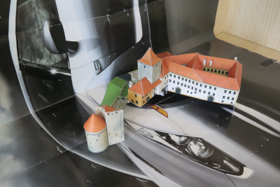
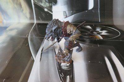
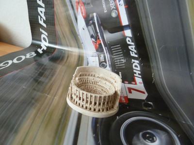
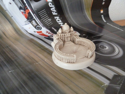
(a) Dal.	(b) Lyc.	(c) Col.	(d) Vat.
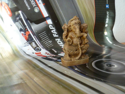
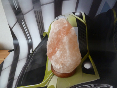
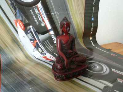
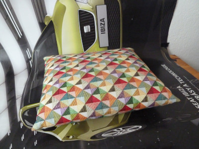
(e) Gan.	(f) Lamp	(g) Bud.	(h) Pil.
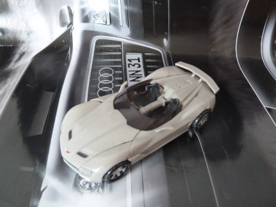
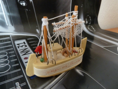
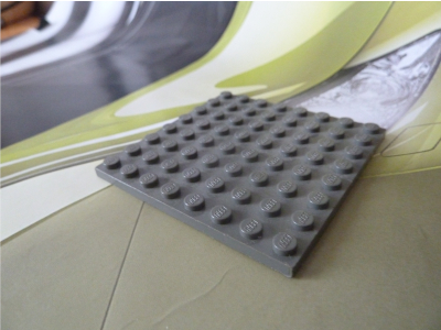
(i) Car	(j) Ship	(k) Cat.	(l) Lego

Dataset	(a)	(b)	(c)	(d)	(e)	(f)
#Takes	8	8	8	8	4	8
#Imgs w. bg.	338	140	294	270	160	330
#Imgs w/o bg.	-	-	326	304	187	302
Dataset	(g)	(h)	(i)	(j)	(k)	(l)
#Takes	8	8	8	8	5	4
#Imgs w. bg.	300	278	329	277	150	264
#Imgs w/o bg.	-	275	290	294	151	307

Figure 4: Sample images from our dataset. For every object, the table shows numbers of takes and images as well as the number of images without background, which are used for the comparison with COLMAP.

4 Experiments

The problem described in this paper has not exactly been considered before, and no datasets existed just for it. Thus first, to demonstrate that our approach delivers good and interesting results, we have created a new dataset, and we evaluate the performance of our method. Our motivation in this experiment is to reconstruct small 3D artifacts and the dataset corresponds to this setting. We considered 12 different scenes, each of which consists of a foreground object and a textured background. We acquired $150$ to $330$ images of every scene; each one was depicted in $4$ - $8$ different configurations (takes), Fig. 4.

4.1 Qualitative results

Fig. 5 shows the results of our method on our dataset. The hyper-parameters were tuned mostly using datasets Daliborka, Lycan, Salt Lamp and Colosseum. The other models were reconstructed with the same settings as the previously mentioned ones. The method did not manage to reconstruct sequence ”Buddha”. We assume, Sec. 3.5, that the first cameras observe the background and the second cameras observe the foreground. This assumption was not met in datasets (e), (h), (k). Hence, the background and the foreground are swapped.

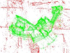
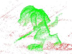
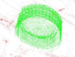
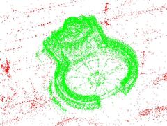
(a) Dal.	(b) Lyc.	(c) Col.	(d) Vat.
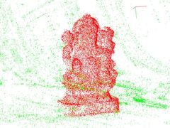
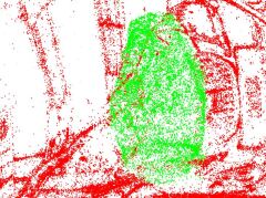
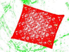
(e) Gan.	(f) Lamp	(g) Bud.	(h) Pil.
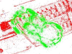
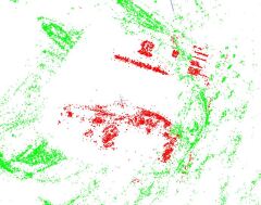
(i) Car	(j) Ship	(k) Cat.	(l) Lego

Figure 5: Results of our metx hod. Foreground is green, background is red.

4.2 Comparison with State-of-the-Art

A direct competitors to our method is hard to do, as this problem had not been really addressed before, but we compare our approach to the most relevant previous approaches.

It makes sense to compare our method to a general approach to motion segmentation and 3D reconstruction. However, as we use unordered input images, we omit the comparison with the methods assuming video input. Also, in our setup, the points are observed by a small portion of cameras, thus the tracks are very sparse, and the track completion is an under-constrained task. The methods based on factorization, therefore, fail, as shows [6], as well as the results of ALC [42], SSC [12] and RSIM [20].

For the motion segmentation, we used six state-of-the-art algorithms: SSC [12], RSIM [20], ALC [42], Subset [71], MODE [2] and YASFM [53]. However, none of the considered methods has produced a satisfactory motion segmentation of sequences from our dataset. SSC outputs wrong results, where almost all points are assigned to one motion. RSIM reports badly conditioned matrices, ALC reports unbounded system during track completion. Subset and MODE run out of memory. If we make the input data shorter, up to 20 images, both Subset and MODE give an incorrect segmentation. YASFM splits the points into more than two models, most of which contain points from both the foreground and the background.

4.3 Comparison with Single body SfM

The motivation for our paper was to find out whether the presence of a background can improve the quality of a model of a given object. To answer this question, we reconstructed the same objects in a classical SfM pipeline COLMAP[49], which is considered to be the state-of-the-art method. COLMAP cannot work with multiple objects, therefore, we run COLMAP on a different dataset with a similar number of images, where the object is depicted without background. The number of the images for the datasets with and without background is in table in Fig. 4.

We compared two metrics: (1) the number of reconstructed points and (2) the median of the reprojection error, Tab. 1. In the case of our method, we count only the points on the foreground.

In the most cases, our method reconstructed models with more points than the standard method. In addition to that, our method achieved lower median reprojection errors for every object. Note, that our method reconstructed the ”Lego” model, which COLMAP could not reconstruct. We can see that the camera poses can be better estimated from a large object with many features when compared to a small object with few features. Thus, the presence of the background in the scene may improve the reconstruction.

4.3.1 Computation time

To compare computation time of TBSfM with the standard SfM, we evaluate the computation times for dataset (e). We get: 2.3 mins feature extraction, 1065 mins feature matching, 14.3 mins 3D reconstruction. Original COLMAP for the same dataset takes 2.3 mins extraction, 449 mins matching, 5.9 mins 3D reconstruction. Our method takes 2.37 times more time in feature matching and 2.4 times more in 3D reconstruction. We solve for two objects, instead of one. It roughly doubles the computation times. Further speedups would be possible if the pipeline was not build on COLMAP but directly designed for multiple objects.

Dataset	Points		Error
	TBSfM	COLMAP	TBSfM	COLMAP
(c)	52397	49418	1.206	1.483
(d)	39024	38833	1.418	1.792
(e)	35179	34539	1.142	1.852
(f)	15305	10049	1.298	1.889
(h)	134086	198728	1.147	2.342
(i)	25229	14372	1.463	2.644
(j)	18244	20571	1.326	1.739
(k)	8004	10143	2.350	2.832
(l)	7692	0	1.818	-

Table 1: Comparison of the number of points and the median reprojection error between our method and COLMAP.

4.4 Experiments with ETH 3D dataset

To further evaluate our method, we have chosen sequences motion_1, motion_2, motion_3 and motion_4 from the SLAM benchmark of the ETH 3D dataset. According to the website of the dataset, sequences motion_3 and motion_4 remain unsolved. These four sequences depict a dynamic scene captured by a rig of two synchronized cameras. Although the objects in the scene perform an independent motion, the objects do not move between any two images taken at the same time by the two cameras of the rig. Therefore, each pair of images taken at the same time builds one take. If we limit ourselves only to such parts of sequence where one object is moving, we may be able to reconstruct the parts of sequences using our method.

We have extracted parts of sequences motion_1, motion_2, motion_3 and motion_4 where there is always one moving object. When compared to our dataset, the images from the ETH 3D dataset have less textured background, worse quality of images, more takes, each of which consists only of two images. In addition to that, there is a person moving the objects, that may confuse the segmentation.

The results of our method on the sequences from the ETH Dataset are in Figure 6. Our method reconstructs and segments all sequences successfully. In most of the results, a person is assigned to the foreground. In sequences (b), (d), (g) the person is not reconstructed. In sequences (a), (i) a person is assigned to the background. In sequence (k) the hand of the person is assigned to the foreground, while the rest of the body is assigned to the background. In sequence (l), the background and the foreground are swapped.

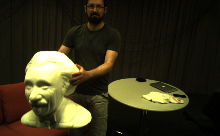
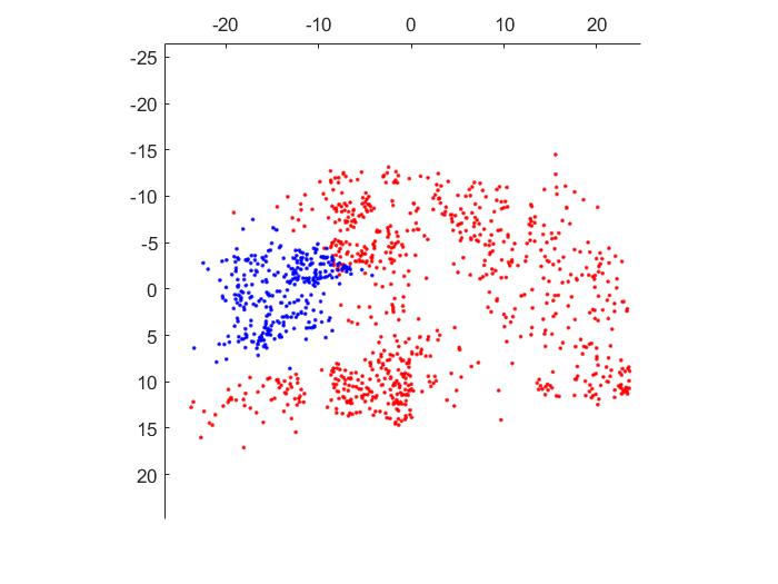
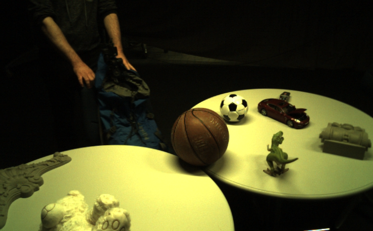
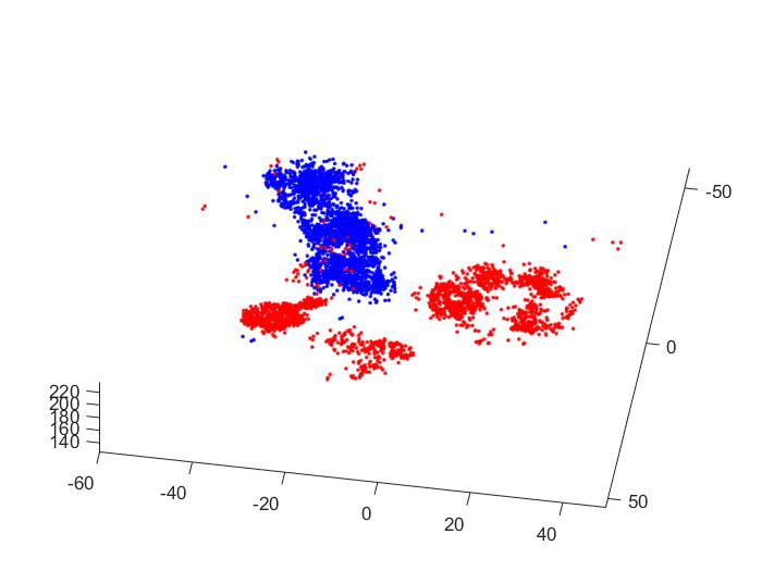
(a)		(b)
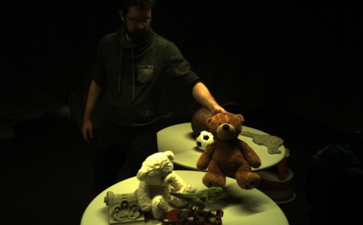
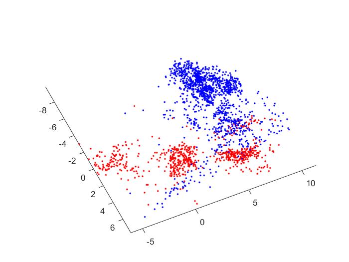
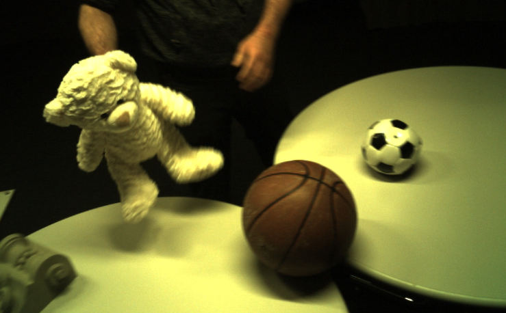
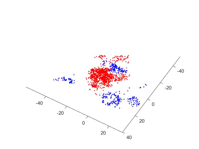
(c)		(d)
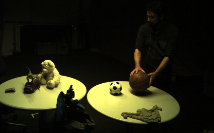
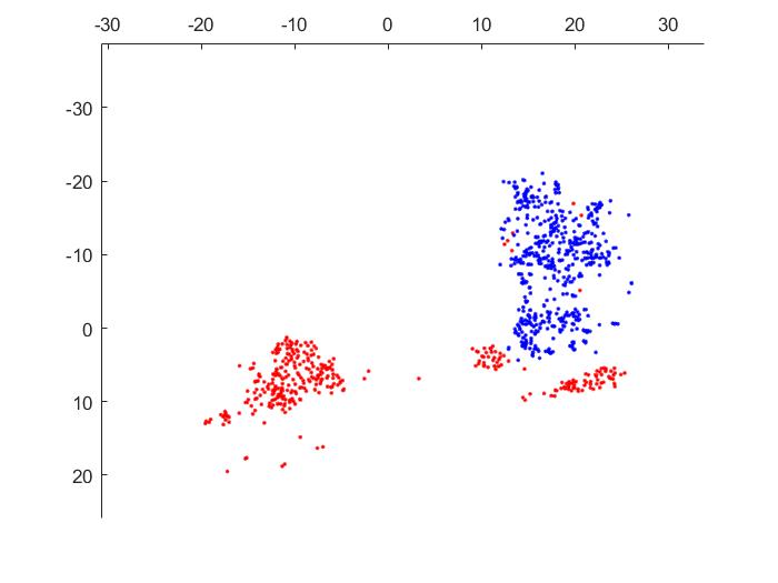
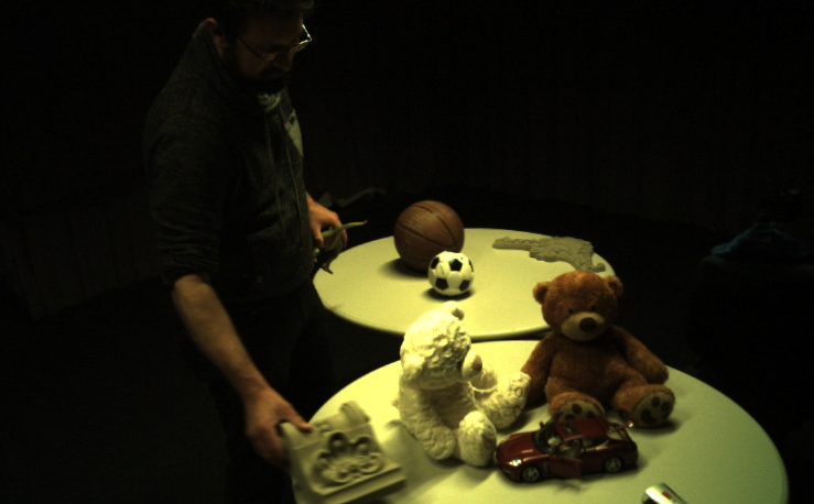
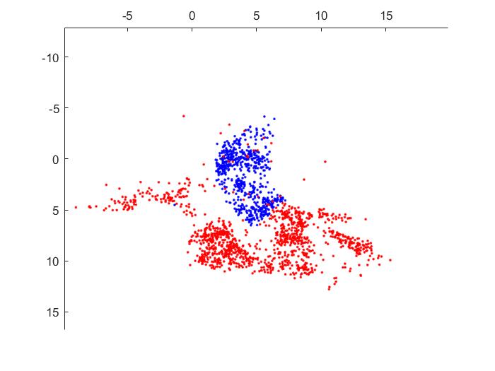
(e)		(f)
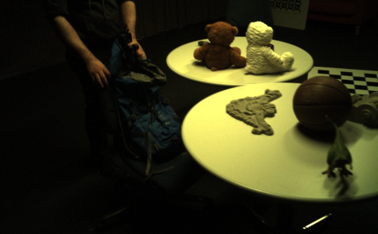
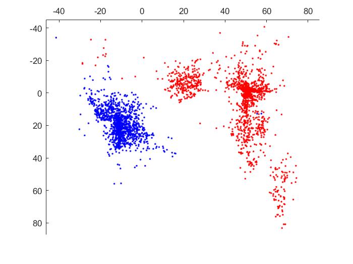
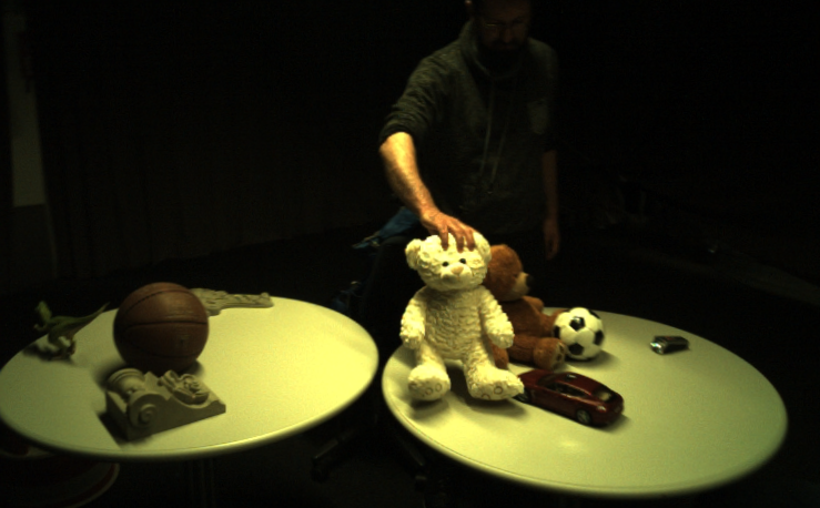
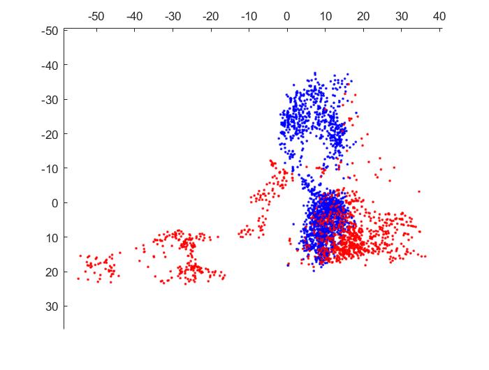
(g)		(h)
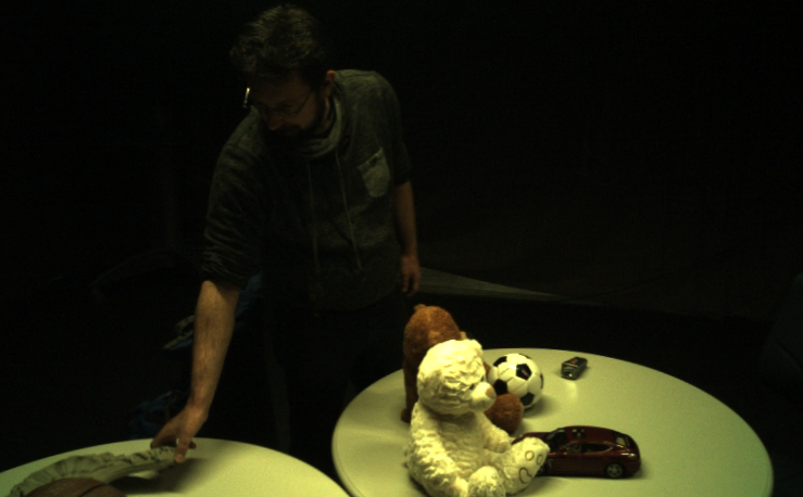
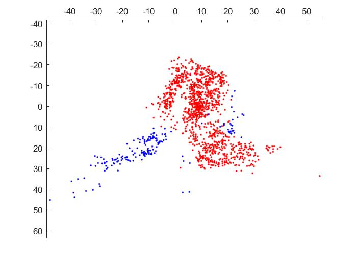
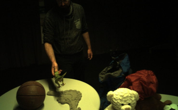
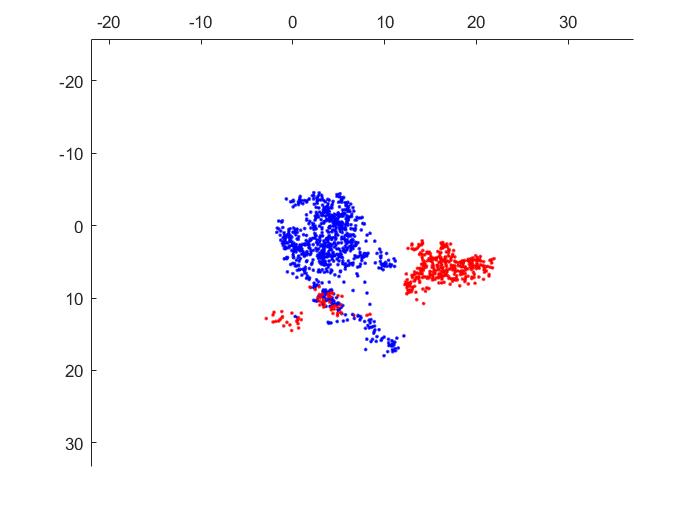
(i)		(j)
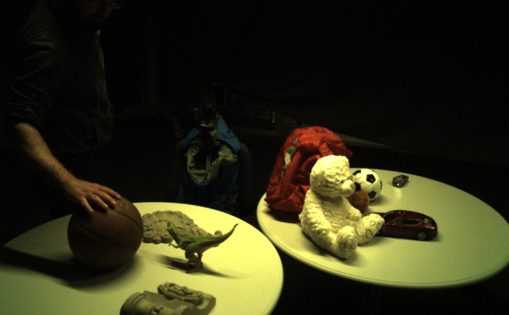
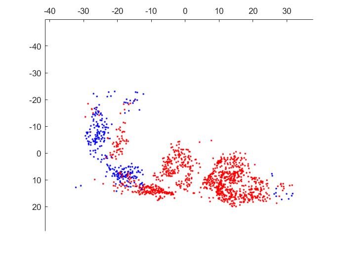
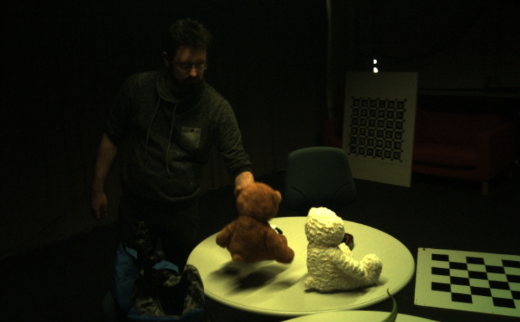
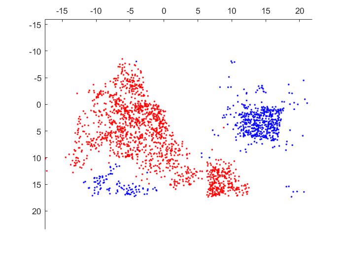
(k)		(l)

Figure 6: Results of our method on the sequences extracted from the ETH 3D dataset. Foreground is blue, background is red.

5 Conclusion

Our TBSfM method for complete 3D reconstruction of objects moving in front of a textured background outperforms the state of the art, Table 1. Real experiments on real data show that it reconstructs objects moving in front of a textured background, Fig. 5, with more points and lower reprojection errors on the objects. All code and data will be made open source.

Reconstructing Small 3D Objects in front of a Textured Background

Here we present additional details, such as experiments and detailed derivations. Sec. 6 contains the experiments with TBSfM. Sec. 6.1 provides a more detailed description of the datasets introduced in Sec. 4 of the main paper, as well as the resulting models reconstructed with TBSfM algorithm. Sec. 6.2 compares the models reconstructed with TBSfM and the models reconstructed with a single-body SfM pipeline [49] from images without background. Sec. 6.3 shows the result of multi-body SfM pipeline YASFM [53] on images from our dataset. Sec. 6.4 shows the result of the segmentation by MODE [2] and Sec. 6.5 shows the result of the segmentation by Subset [71]. Sec. 6.6 shows the model which outputs a single-body SfM pipeline COLMAP [49], if it is given images from different takes. Sec 6.7 contains the experiments conducted with ETH 3D dataset [50].

Sec. 7 contains the derivation of the formula for foreground motion, which is used in Sec. 8. Sec. 8 describes an additional criterion for local observation grouping, which is based on the foreground motion. Sec. 9 contains the derivation of the formula for transformation of points between reconstructed models, which is used in Sec. 10. Sec. 10 describes transformation of the cameras, which is used in Sec. 3.6 of the main paper.

Code in C++ is available on Github. Please, follow the readme file to compile and run a representative experiment.

6 Experiments

6.1 Datasets and results of TBSfM

In this section we give a detailed description of the datasets introduced in Sec. 4 of the main paper. We provide a further view on the models reconstructed by TBSfM from our datasets, which are described in Sec. 4.1 in the main paper.

Table 2 describes the properties of the datasets, such as the number of takes, the number of images and special characteristics of the objects (planar, repetitive, …) or the datasets (translational motion only). Properties of the reconstructed models are shown in Table 3.

The images of the scenes together with the results of TBSfM on them are shown in Figures 7, 8, 9, 10. In each row, the image on the left is an image taken from the dataset, while the image on the right depicts the 3D model reconstructed from the dataset with TBSfM. TBSfM was not able to reconstruct the dataset ”Buddha” (Fig. 9(c)), due to the small density of features, reflections on the surface of the object and small overlaps between neighboring takes. Other models were reconstructed successfully. The points assigned to the foreground are displayed green, while the points assigned to the background are red. Figures 7(h), 8(f), 9(d) show that if the foreground is dominant, it may be swapped with the background. Figures 7, 8, 9, 10 show that the quality of the segmentation, as well as the quality of the reconstruction is high.

Foreground	Background	Takes	Images	Special	Figure
Daliborka	Nissan GTR	8	338	NONE	7(a)
Lycan	Nissan GTR	8	140	NONE	8(a)
Colosseum	Peugeot 908	8	294	NONE	8(c)
Vatican	Peugeot 908	8	270	NONE	8(e)
Ganesha	Peugeot 908	4	160	Only translation	8(g)
Salt lamp	Seat Ibiza	8	330	Translucent	9(a)
Buddha	Peugeot 908	8	300	Shiny	9(c)
Pillow	Seat Ibiza	8	278	Repetitive	9(e)
Car	Audi S8	8	329	NONE	9(g)
Ship	Audi S8	8	277	NONE	10(a)
Catalog	Seat Ibiza	5	150	Planar	10(c)
Lego	Seat Ibiza	4	264	Repetitive, Planar	10(e)

Table 2: Properties of the datasets.

Dataset	Figure	Points Fg.	Points Bck.	Swapped
Daliborka	7(b)	37755	26324	NO
Lycan	8(b)	40347	12345	NO
Colosseum	8(d)	52397	33335	NO
Vatican	8(f)	39024	35160	NO
Ganesha	8(h)	35179	40643	YES
Salt lamp	9(b)	15305	63828	NO
Pillow	9(d)	134086	30532	YES
Car	9(f)	25229	46878	NO
Ship	10(h)	18244	21983	NO
Catalog	10(b)	8004	20757	YES
Lego	10(d)	7692	29964	NO

Table 3: Results of the reconstructions.

(a)	(b)

Figure 7: Reconstructed datasets, Part 1.

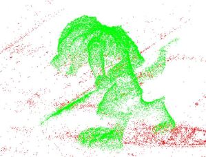
(a)	(b)
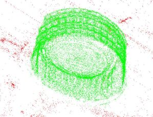
(c)	(d)
(e)	(f)
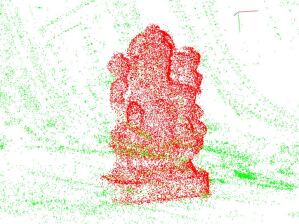
(g)	(h)

Figure 8: Reconstructed datasets, Part 2.

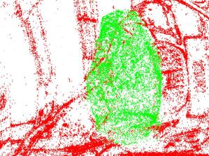
(a)	(b)
(c)	(d)
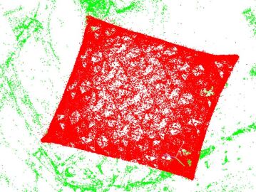
(e)	(f)
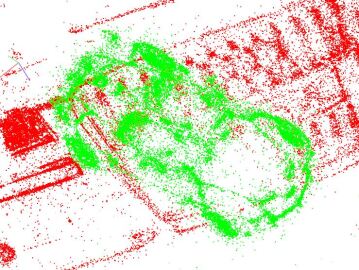
(g)	(h)

Figure 9: Reconstructed datasets, Part 3.

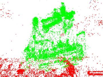
(a)	(b)
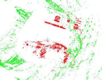
(c)	(d)
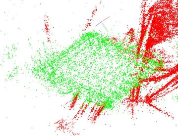
(e)	(f)

Figure 10: Reconstructed datasets, Part 4.

6.2 Comparison with single body SfM

This section shows the result of the comparison proposed in Sec. 4.3 of the main paper. We show, for which kinds of objects and how much, TBSfM improves the reconstruction. We have created sets of photographs of the same objects but this time without any background, like in Figure 11. We compare the models reconstructed with TBSfM on the data with background and the models of the same objects reconstructed with state-of-the-art SfM pipeline COLMAP [49] without the background. We measure two quantities: the number of reconstructed points and the median reprojection error.

Table 4 compares the numbers of reconstructed points and the median reprojection error. In the results of TBSfM, only the points from the foreground are assumed. In 6 out of 9 cases the model reconstructed with TBSfM has more points than the model reconstructed without the background, including model ”Lego”, which the state-of-the-art pipeline COLMAP did not manage to reconstruct without the background. Table 4 shows that TBSfM achieved lower median reprojection error for all considered models.

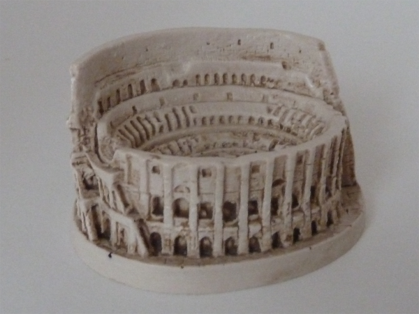
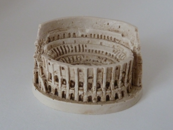
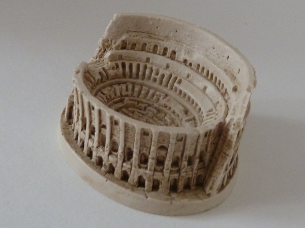
Figure 11: Example of the images of an object without the background.

Dataset	Points		Error
	TBSfM	COLMAP	TBSfM	COLMAP
Colosseum	52397	49418	1.206	1.483
Vatican	39024	38833	1.418	1.792
Ganesha	35179	34539	1.142	1.852
Salt lamp	15305	10049	1.298	1.889
Pillow	134086	198728	1.147	2.342
Car	25229	14372	1.463	2.644
Ship	18244	20571	1.326	1.739
Catalog	8004	10143	2.350	2.832
Lego	7692	0	1.818	-

Table 4: Comparison of the number of points and the median reprojection error between TBSfM and COLMAP.

Figures 12, 13, 14 compare the models of the objects reconstructed with TBSfM and with COLMAP. In each row, the image on the left depicts a model of the foreground object reconstructed using TBSfM, while the image on the right depicts model of the same object reconstructed in COLMAP without background. TBSfM reconstructed significantly denser models of objects ”Ganesha” (Fig. 12(e)), ”Lamp” (Fig. 13(a)) and ”Car” (Fig. 13(e)). Also notice, that TBSfM managed to reconstruct some parts of objects, which COLMAP could not reconstruct, like the wall on the back side of the ”Vatican” object (Fig. 12(c)) or the base of the ”Lamp” object (Fig. 13(a)). In addition to that, TBSfM managed to reconstruct object ”Lego” (Fig. 14(e)), which could not be reconstructed by COLMAP without the background due to its planar and repetitive shape. On the other hand, COLMAP reconstructed better models of objects ”Ship” (Fig. 14(a)) and ”Catalog” (Fig. 14(c)).

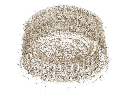
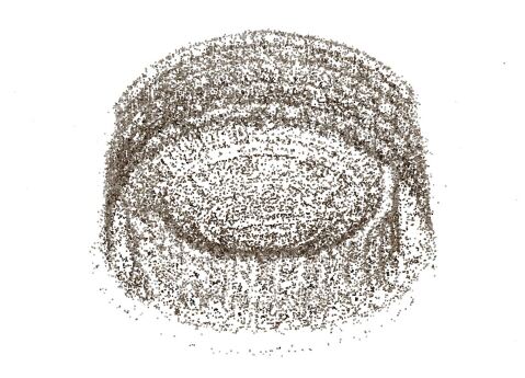
(a)	(b)
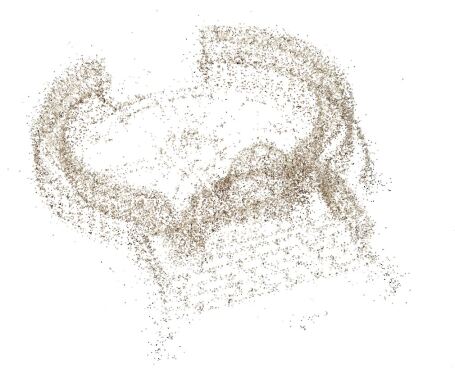
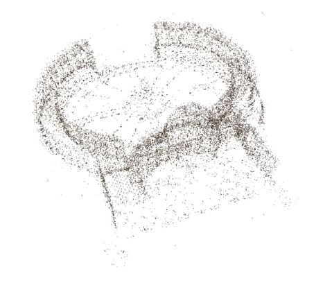
(c)	(d)
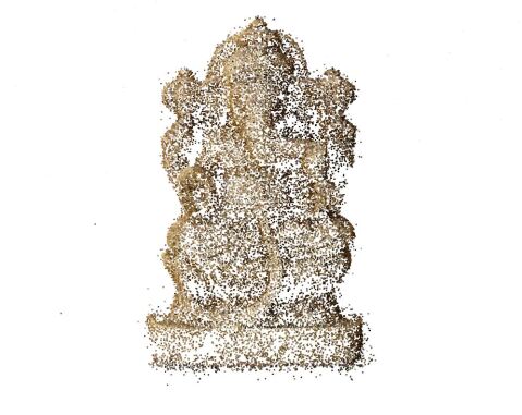
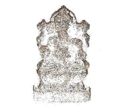
(e)	(f)

Figure 12: Comparison of the models reconstructed with and without the background. The models on the left side have been reconstructed with the background.

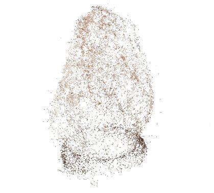
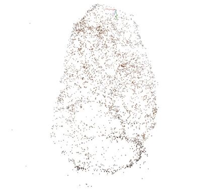
(a)	(b)
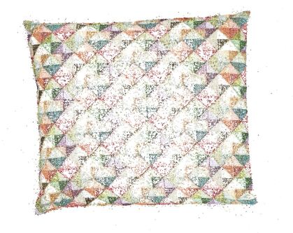
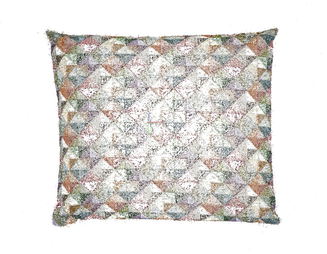
(c)	(d)
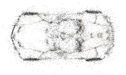
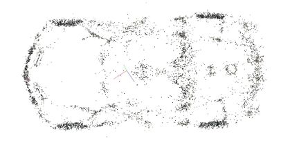
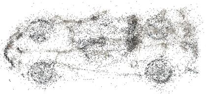
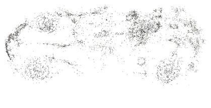
(e)	(f)

Figure 13: Comparison of the models reconstructed with and without the background. The models on the left side have been reconstructed with the background.

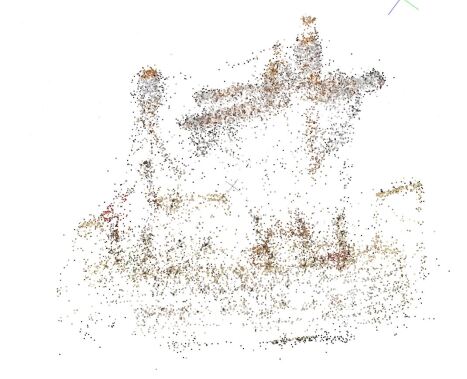
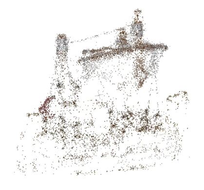
(a)	(b)
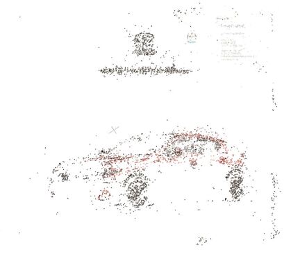
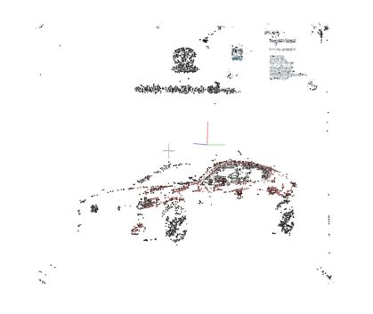
(c)	(d)
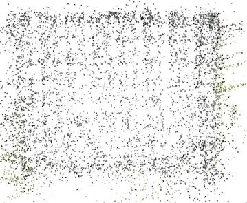
(e)	(f)

Figure 14: Comparison of the models reconstructed with and without the background. The models on the left side have been reconstructed with the background.

6.3 Results of YASFM

In this section we give an example of the result, which outputs a MBSfM pipeline YASFM [53], if it is given the images from our dataset. Figure 15 shows that YASFM typically splits the model into more than two objects, most of which contain points from both the foreground and the background. For example the reconstruction of the ”Daliborka” object was split into five models, which are shown in Figure 15. Figures 15(a), 15(b), 15(c) show models which contain points from both the foreground and the background. Figures 15(d), 15(e) show very sparse models. The result of our method on this dataset is shown in Figure 7(b).

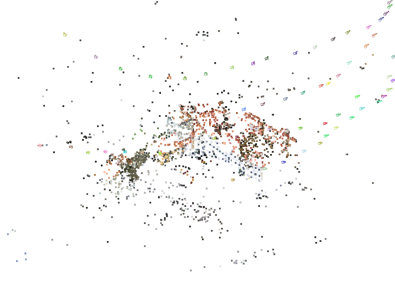
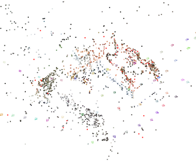
(a)	(b)
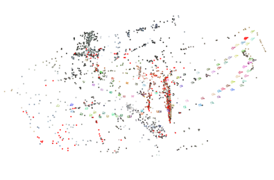
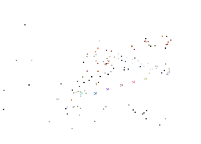
(c)	(d)
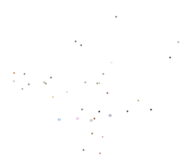
(e)

Figure 15: Models reconstructed from Daliborka dataset in YASFM. The reconstruction has split into five models.

6.4 Results of MODE

In this section we give an example of the result of the segmentation, which outputs MODE [2], if it is given the images from our dataset. If the whole datasets are used as the input, MODE runs out of memory. We have, therefore, shortened our dataset to 7 images, which were used as the input for the method. Figure 16 shows that the result of the segmentation is not correct and that both clusters contain points from the foreground object, as well as from the background. Our method is able to correctly segment and reconstruct the shortened version of the dataset, the result of our method is shown in Figure 17.

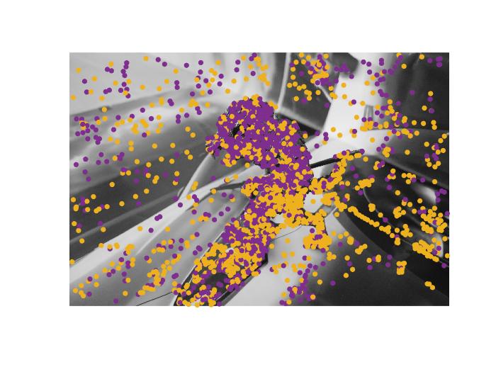
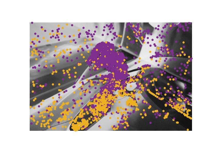
(a)	(b)
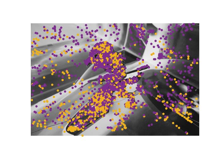
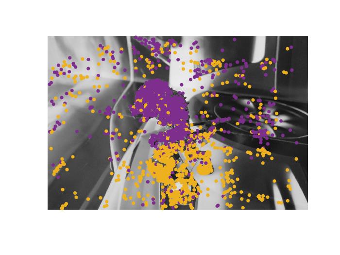
(c)	(d)

Figure 16: Result of motion segmentation by MODE. Points belonging to the first object are purple and points belonging to the second object are yellow.

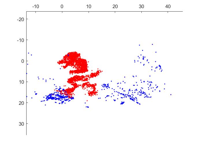
Figure 17: Result of our method on the shortened version of Lycan dataset. Although the total number of images is equal to 7, our method gives a meaningful result.

6.5 Results of Subset

In this section we give an example of the result of the segmentation, which outputs Subset [71] if it is given the images from our dataset. If the whole datasets are used as the input, Subset runs out of memory. Therefore, we have shortened our dataset to 7 images, which were used as the input for the method. Paper [71] describes six different spectral clustering schemes to fuse the clustering information: (a) Affine, (b) Homography, (c) Fundamental, (d) Kernel Addition, (e) Co-Regularization, (f) Subset Constrained Multi-View Spectral Clustering. All the schemes assign all the points to one object. If we enforce 2 objects, all spectral clustering schemes give incorrect segmentation results, which are shown in Figure 18. Our method is able to correctly segment and reconstruct the shortened version of the dataset, the result of our method is shown in Fig. 17.

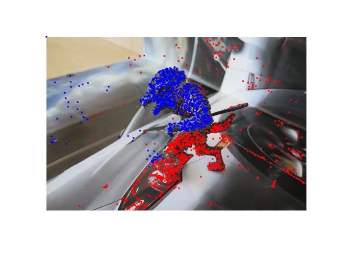
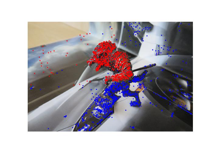
(a)	(b)
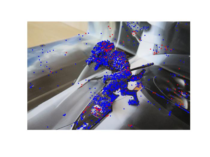
(c)	(d)
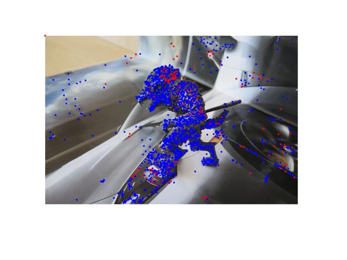
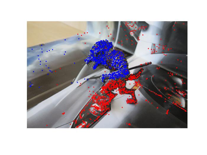
(e)	(f)

Figure 18: Result of motion segmentation by Subset. Points belonging to the first object are blue and points belonging to the second object are red. Particular images are results of (a) Affine, (b) Homography, (c) Fundamental, (d) Kernel Addition, (e) Co-Regularization, (f) Subset Constrained Multi-View Spectral Clustering.

6.6 Results of COLMAP

In this section we show the result, which outputs the single body SfM pipeline COLMAP [49], if it is given images from different takes. COLMAP is not able to segment the points from different objects. The section is related to Sec. 4.2 of the main paper. We see in Figure 19 that the resulting model contains one background, on which the foreground object is reconstructed multiple times on different positions, once for each take.

Figure 19: Model reconstructed from the whole Daliborka dataset in COLMAP.

6.7 Experiments with ETH 3D dataset

In this section we show the result of the experiments with the sequences, which have been extracted from the ETH 3D SLAM datasets [50]. The experiment has been proposed in Sec. 4.4 of the main paper. The sequences have been extracted from datasets motion_1, motion_2, motion_3, motion_4, which depict a dynamic scene with a synchronized rig of two cameras. Although the objects in the scene perform an independent motion, the objects do not move between any two images taken at the same time by the two cameras of the rig. Therefore, we obtain the semi-dynamic setting, where each pair of images taken at the same time builds one take. We have extracted every sequence in such a way that it contains one object moving with respect to the background. The properties of the sequences are in Table 5.

ID	Dataset	Object	First Image	Last Image	Length
(a)	motion_1	Einstein Bust	7603.638892	7607.214650	98
(b)	motion_2	Backpack	7978.918332	7981.867380	130
(c)	motion_3	Brown Bear	8020.794811	8024.628573	105
(d)	motion_3	White Bear	8005.828393	8007.855864	56
(e)	motion_3	Ball	8012.353162	8017.403406	138
(f)	motion_3	Frieze 1	8028.019978	8032.885907	133
(g)	motion_4	Backpack	8086.964071	8088.991541	56
(h)	motion_4	White Bear	8075.094154	8076.863582	49
(i)	motion_4	Frieze 2	8077.674570	8081.508333	105
(j)	motion_4	Dinosaur	8107.607406	8110.150959	70
(k)	motion_4	Ball	8111.478031	8114.021584	70
(l)	motion_4	Brown Bear	8132.637449	8138.277503	154

Table 5: Properties of the sequences extracted from ETH 3D dataset, which have been used to evaluate our method.

The quality of the images in these sequences is lower than in the case of our dataset, the images are darker and every take contains only two images. Moreover, the scene contains the person, who moves the objects. Still, our method is able to reconstruct these scenes and segment the objects. Examples of the images from the sequences together with the results are shown in Figure 20. The properties of the resulting models are shown in Table 6. In the most of the cases, the person is segmented together with the foreground, as in the sequences the person moves together with the foreground object. In sequences (a), (i) the person is segmented together with the background. In sequences (b), (c), (d), (g) the person is not reconstructed. In sequence (k) the hand of the person is assigned to the foreground, while the rest of the body is assigned to the background. In sequence (l), the background and the foreground are swapped. Model (c) has been reconstructed together with its shadow.

The results on the sequences extracted from the ETH 3D dataset show, that our method is able to reconstruct and segment scenes which are less controlled than the scenes from our dataset. It also shows, that although our semi-dynamic setting may seem to be too restrictive and impractical, it indeed has a practical use when reconstructing fully dynamic scenes observed by multiple synchronized cameras.

ID	Figure	$\#$Points Fg.	$\#$Points Bck.	Person	Swapped
(a)	20 (a)	353	1015	background	NO
(b)	20 (b)	2734	2345	not reconstructed	NO
(c)	20 (c)	1402	852	not reconstructed	NO
(d)	20 (d)	1130	382	not reconstructed	YES
(e)	20 (e)	616	539	foreground	NO
(f)	21 (a)	624	1206	foreground	NO
(g)	21 (b)	2091	2073	not reconstructed	NO
(h)	21 (c)	2042	1362	foreground	NO
(i)	21 (d)	233	1337	background	NO
(j)	21 (e)	891	442	foreground	NO
(k)	22 (a)	314	1202	split, hand with Fg.	NO
(l)	22 (b)	1564	793	foreground	YES

Table 6: Results of the models reconstructed from the sequences extracted from ETH 3D dataset.

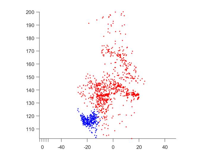
	(a)
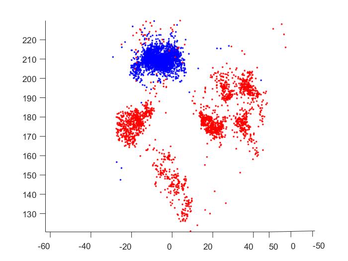
	(b)
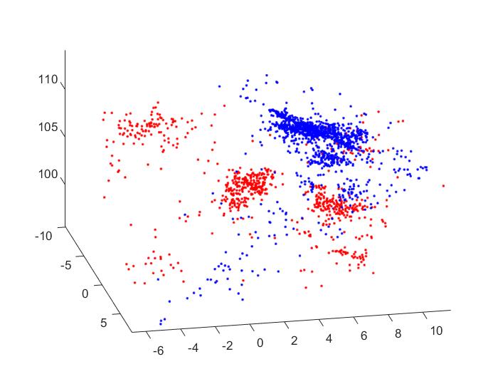
	(c)
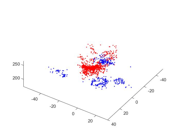
	(d)
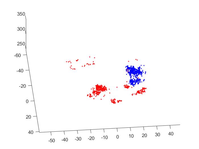
	(e)

Figure 20: Results of our method on the sequences extracted from the ETH Dataset. Left: image from the sequence, Middle: front view, Right: top view.

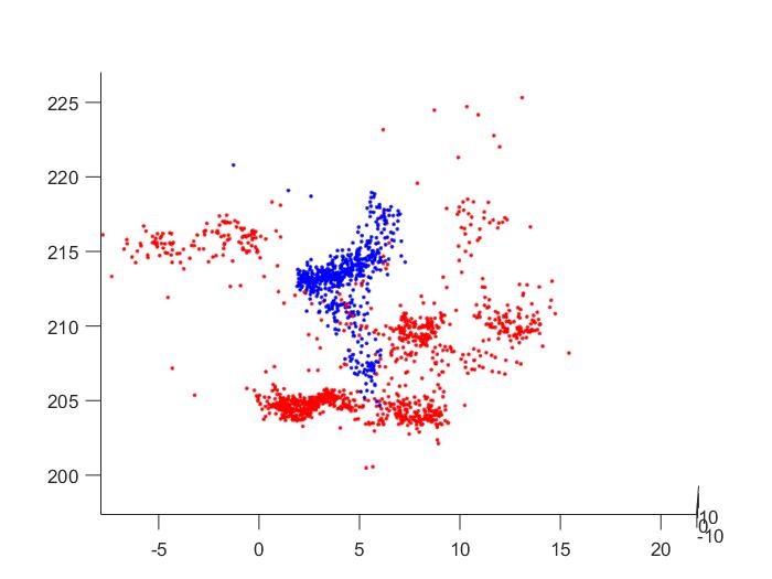
	(a)
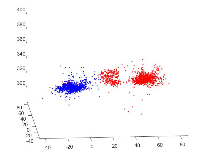
	(b)
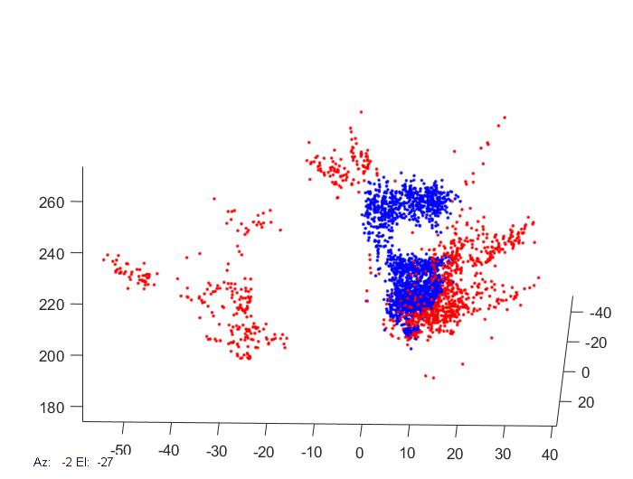
	(c)
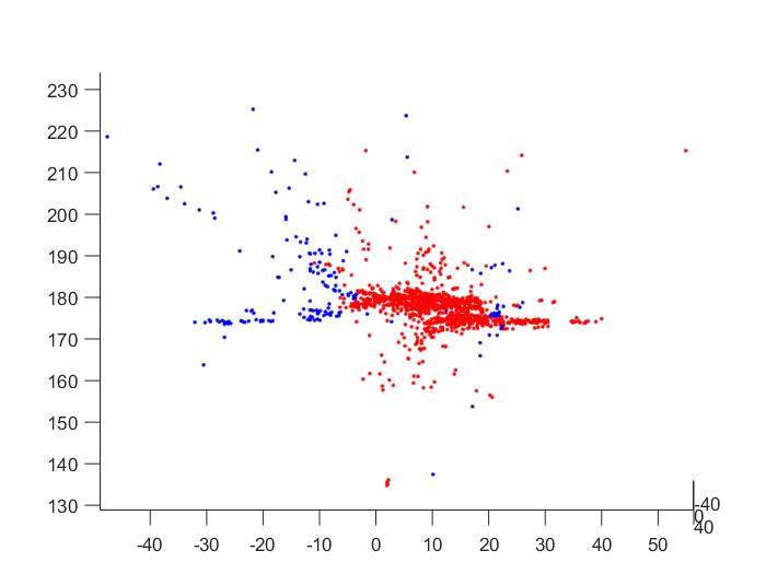
	(d)
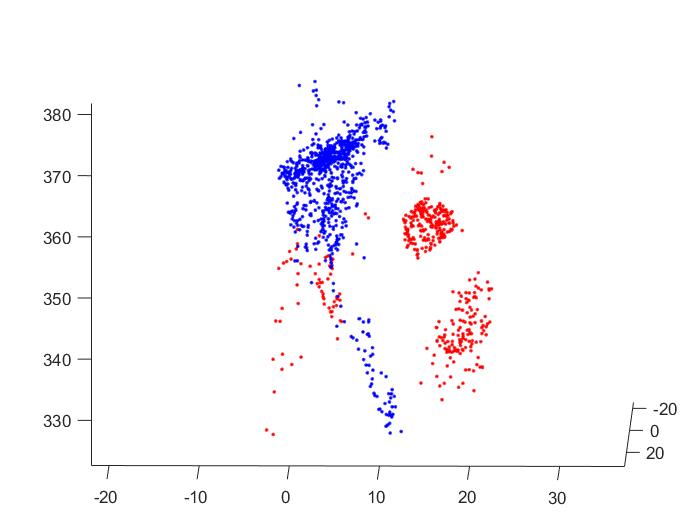
	(e)

Figure 21: Results of our method on the sequences extracted from the ETH Dataset. Left: image from the sequence, Middle: front view, Right: top view.

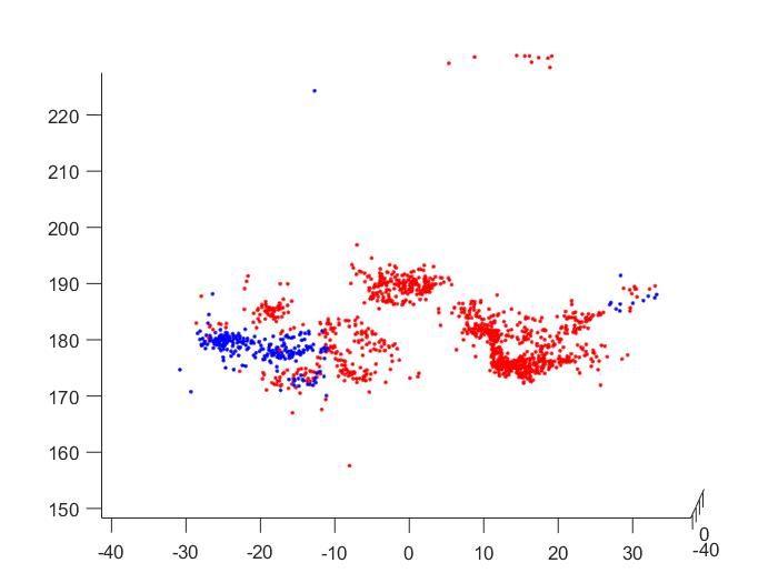
	(a)
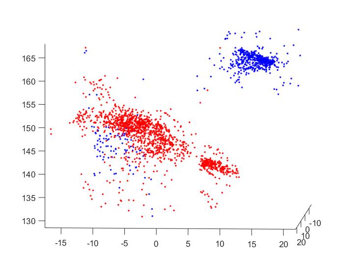
	(b)

Figure 22: Results of our method on the sequences extracted from the ETH Dataset. Left: image from the sequence, Middle: front view, Right: top view.

7 Foreground motion calculation

In this section we show that we can compute the motion $(A_{t,s,\delta_{t}}^{F},a_{t,s,\delta_{t}}^{F})$ of the foreground from a camera pair ($P_{s,\delta_{t}}^{j_{s},B},P_{s,\delta_{t}}^{j_{s},F}$) obtained with the sequential registration of an image $P_{s,\delta_{s}}^{j_{s}}$ capturing configuration $s$ towards model of configuration $t$. Camera $P_{s,\delta_{t}}^{j_{s},B}$ is registered towards the background while $P_{s,\delta_{t}}^{j_{s},F}$ is registered towards the foreground. The computed motion is in coordinate system $\delta_{t}$. The result is used in Sec. 3.3 of the main paper.

Let $X_{s,i,\delta_{s}}^{F}$ be a point from the foreground in model of take $s$. Let $x_{s,i}^{F,j_{s}}$ be the projection of $X_{s,i,\delta_{s}}^{F}$ onto camera $P_{s,\delta_{s}}^{j_{s}}$.

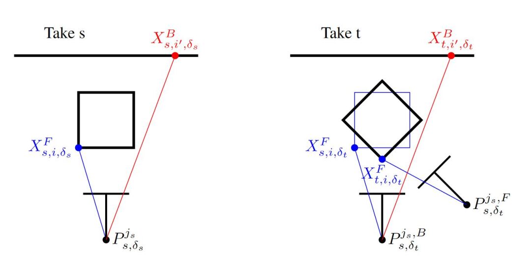
Figure 23: Example of a camera from take $s$ after the sequential PnP registration towards take $t$.

Figure 23 shows that if camera $P_{s,\delta_{s}}^{j_{s}}$ from take $s$ is registered towards the foreground points from model of take $t$, it projects the foreground points from model of take $t$ onto the same 2D points onto which they are projected in the model of take $s$. Let $X_{t,i,\delta_{t}}^{F}$ be reconstruction of point $X_{s,i,\delta_{s}}^{F}$ in model of take $t$. Then $x_{s,i}^{F,j_{s}}$ is a projection of point $X_{t,i,\delta_{t}}^{F}$ into camera $P_{s,\delta_{t}}^{j_{s},F}$

Figure 23 also shows that if the same camera $P_{s,\delta_{s}}^{j_{s}}$ from the second take is registered towards the background points from the model of take $t$, the position of the camera towards the background is the same as in take $s$. This means that if a foreground point is transformed to the configuration of take $s$, it will be projected onto the same 2D feature onto which it is projected in take $s$. Let $X_{s,i,\delta_{t}}^{F}=A_{t,s,\delta_{t}}^{F}X_{t,i,\delta_{t}}^{F}+a_{t,s,\delta_{t}}^{F}$ be point $X_{t,i,\delta_{t}}^{F}$ in coordinate system $\delta_{t}$ and position of take $s$. Then $x_{s,i}^{F,j_{s}}$ is a projection of point $X_{s,i,\delta_{t}}^{F}$ onto camera $P_{s,\delta_{t}}^{j_{s},B}$.

The following equation must therefore hold true:

$$\alpha P_{s,\delta_{t}}^{j_{s},F}\begin{bmatrix}X_{t,i,\delta_{t}}^{F}\\ 1\end{bmatrix}=\alpha P_{s,\delta_{t}}^{j_{s},B}\begin{bmatrix}X_{s,i,\delta_{t}}^{F}\\ 1\end{bmatrix}\\$$ (12)

We can replace $X_{s,i,\delta_{t}}^{F}$ with $A_{t,s,\delta_{t}}^{F}X_{t,i,\delta_{t}}^{F}+a_{t,s,\delta_{t}}^{F}$ and rewrite the equation using symbols for rotation, center and camera calibration matrix for cameras $P_{s,\delta_{t}}^{j_{s},F}$ and $P_{s,\delta_{t}}^{j_{s},B}$ as:

$$\alpha KR_{s,\delta_{t}}^{j_{s},F}(X_{t,i,\delta_{t}}^{F}-c_{s,\delta_{t}}^{j_{s},F})=\alpha KR_{s,\delta_{t}}^{j_{s},B}(A_{t,s,\delta_{t}}^{F}X_{t,i,\delta_{t}}^{F}+a_{t,s,\delta_{t}}^{F}-c_{s,\delta_{t}}^{j_{s},B})$$ (13)

We can eliminate $K$ and $\alpha$ and replace :

$$R_{s,\delta_{t}}^{j_{s},F}(X_{t,i,\delta_{t}}^{F}-c_{s,\delta_{t}}^{j_{s},F})=R_{s,\delta_{t}}^{j_{s},B}(A_{t,s,\delta_{t}}^{F}X_{t,i,\delta_{t}}^{F}+a_{t,s,\delta_{t}}^{F}-c_{s,\delta_{t}}^{j_{s},B})$$ (14)

Because the equation has to hold true for all $X_{t,i,\delta_{t}}^{F}$, it holds true also for $X_{t,i,\delta_{t}}^{F}=0$, which implies that the following two equations also hold true:

$$-R_{s,\delta_{t}}^{j_{s},F}c_{s,\delta_{t}}^{j_{s},F}=R_{s,\delta_{t}}^{j_{s},B}a_{t,s,\delta_{t}}^{F}-R_{s,\delta_{t}}^{j_{s},B}c_{s,\delta_{t}}^{j_{s},B}\\$$ (15)

$$R_{s,\delta_{t}}^{j_{s},F}=R_{s,\delta_{t}}^{j_{s},B}A_{t,s,\delta_{t}}^{F}\\$$ (16)

We can easily find the relative rotation $A_{t,s,\delta_{t}}^{F}$ from the latter equation as

$$A_{t,s,\delta_{t}}^{F}=(R_{s,\delta_{t}}^{j_{s},B})^{-1}R_{s,\delta_{t}}^{j_{s},F}\\$$ (17)

We can substitute (17) into (15) to obtain:

$$-R_{s,\delta_{t}}^{j_{s},F}c_{s,\delta_{t}}^{j_{s},F}=R_{s,\delta_{t}}^{j_{s},B}a_{t,s,\delta_{t}}^{F}-R_{s,\delta_{t}}^{j_{s},B}c_{s,\delta_{t}}^{j_{s},B}\\$$ (18)

We can find translation $a_{t,s,\delta_{t}}^{F}$ as

$$a_{t,s,\delta_{t}}^{F}=c_{s,\delta_{t}}^{j_{s},B}-A_{t,s,\delta_{t}}^{F}c_{s,\delta_{t}}^{j_{s},F}\\$$ (19)

We can compute the motions of the foreground from take $s$ to take $t$ according to equations (17), (19), if we have a pair of cameras obtained with sequential registration of a camera $P_{s,\delta_{s}}^{j_{s}}$ towards take $t$. One camera pair is enough for finding the relative motion.

8 Additional criterion for local observation grouping

Local observation grouping, which is based on common observed points, is described in Main paper in Section 3.3. In this section, we describe an additional criterion, which is based on the motion of the object. This criterion compares the motion of the object, which is computed from the pair of sequentially registered cameras according to Section 7. As this criterion requires multiple pairs from the same take to be registered towards the current take, it is suitable for datasets, where every take contains many images. Now, we will show that the cameras can be clustered by the motion of the foreground, which can be computed from the sequentially registered poses.

If poses $P_{s,\delta_{t}}^{j_{s},B}$ and $P_{s,\delta_{t}}^{j_{s},F}$ are known, the motion $(A_{t,s,\delta_{t}}^{F},a_{t,s,\delta_{t}}^{F})$ can be computed by (17), (19). Note that the motion (17), (19) is in coordinate system $\delta_{t}$ of take $t$.

Let us have two different poses $P_{s,\delta_{t}}^{j_{s},1},P_{s,\delta_{t}}^{j_{s},2}\in\mathcal{P}_{s,\delta_{t}}^{j_{s}}$ of the same camera $P_{s,\delta_{s}}^{j_{s}}$ Suppose that we follow formulas (17), (19) to compute the motion. Four different situations can occur

1. Forward motion Pose $P_{s,\delta_{t}}^{j_{s},1}$ observes the background and pose $P_{s,\delta_{t}}^{j_{s},2}$ observes the foreground; then formulas (17), (19) give motion $(A_{t,s,\delta_{t}}^{F},a_{t,s,\delta_{t}}^{F})$.

2. Backward motion Pose $P_{s,\delta_{t}}^{j_{s},1}$ observes the foreground and pose $P_{s,\delta_{t}}^{j_{s},2}$ observes the background. It can be easily shown that formulas (17), (19) give motion $(A_{s,t,\delta_{t}}^{F},a_{s,t,\delta_{t}}^{F})$, which is the inverse of the original motion $(A_{t,s,\delta_{t}}^{F},a_{t,s,\delta_{t}}^{F})$.

3. Zero motion Both poses observe the same object; formulas (17), (19) give zero motion, i.e.,  it is close to $(I,0)$.

4. Wrong result At least one of the poses is badly estimated, (17), (19) give a result different from the previous ones.

For given takes $s$, $t$ we select all the sets of poses $\mathcal{P}_{s,\delta_{t}}^{j_{s}},j_{s}\in[1,m_{s}]$ obtained with sequential registration of cameras from take $s$ towards take $t$. From each of these sets, we extract camera pairs $P_{s,\delta_{t}}^{j_{s},1},P_{s,\delta_{t}}^{j_{s},2}$ and then we compute the motion from these camera pairs using formulas (17), (19).

The computed motions cluster around the correct motion values $(A_{t,s,\delta_{t}}^{F},a_{t,s,\delta_{t}}^{F})$, $(A_{s,t,\delta_{t}}^{F},a_{t,s,\delta_{t}}^{F})$, $(0,I)$, Fig. 24. First, we remove the zero motions with spectral clustering [67]. Then, we use Sequential RANSAC to find the clusters of the forward motions and the backward motions.

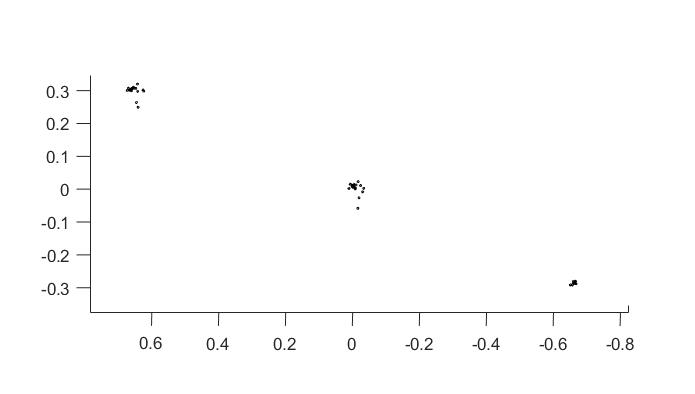
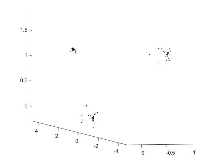
(a)	(b)

Figure 24: Euler vectors (a) and translations (b) of the motions calculated with (17), (19). Three clusters representing the forward, backward and zero motions are observable.

For every two takes $s$, $t$, $s\neq t$, we have obtained clusters $\mathcal{C}_{s,t}^{l},l\in[1,q_{s,t}]$ of ordered camera pairs. In the forward motion cluster, the first camera in a pair observes the background and the second one observes the foreground. In the backward motion cluster it is vice versa. We can merge the clusters which observe the same reconstruction using the linkage scheme described in Sec 3.3 of the main paper. Then, the clusters obtained in Sec 3.3 of the main paper, are further merged according to Sec 3.5 of the main paper.

9 Calculation of transformation of points between takes

In this section we compute transformation $(B_{s,t}^{o},b_{s,t}^{o},\beta_{s,t}^{o})$ of the points of object $o$ from model of take $s$ to model of take $t$ from a camera $P_{s,\delta_{s}}^{j_{s}}$ from take $s$ and its pose $P_{s,\delta_{t}}^{j_{s},o}$ registered towards object $o$ in model of take $t$. The result of this section is used in Section 10.

Let $X_{s,i,\delta_{s}}^{o}$ be an arbitrary point from object $o$ in model of take $s$. Let $X_{t,i,\delta_{t}}^{o}$ be the point $X_{s,i,\delta_{s}}^{o}$ in model of take $t$. Then, there holds true:

$$X_{t,i,\delta_{t}}^{o}=\beta_{s,t}^{o}B_{s,t}^{o}X_{s,i,\delta_{s}}^{o}+b_{s,t}^{o}$$ (20)

The 3D point is projected onto the same point on the camera in both reconstructions, so there holds true:

$$\overrightarrow{x}=\alpha P_{s,\delta_{t}}^{j_{s},o}\begin{bmatrix}X_{t,i,\delta_{t}}^{o}\\ 1\end{bmatrix}=\alpha P_{s,\delta_{s}}^{j_{s}}\begin{bmatrix}X_{s,i,\delta_{s}}^{o}\\ 1\end{bmatrix}$$ (21)

We assume that both poses belong to the same camera, so the camera calibration matrix $K$ is the same for both pictures. We rewrite the equation using symbols for rotation, center and camera calibration matrix as:

$$\alpha_{1}KR_{s,\delta_{t}}^{j_{s},o}(X_{t,i,\delta_{t}}^{o}-c_{s,\delta_{t}}^{j_{s},o})=\alpha_{2}KR_{s,\delta_{s}}^{j_{s}}(X_{s,i,\delta_{s}}^{o}-c_{s,\delta_{s}}^{j_{s}})$$ (22)

We eliminate $K$, introduce $\sigma=\frac{\alpha_{1}}{\alpha_{2}}$ and replace $X_{t,i,\delta_{t}}^{o}$ with $\beta_{s,t}^{o}B_{s,t}^{o}X_{s,i,\delta_{s}}^{o}~{}+~{}b_{s,t}^{o}$:

$$\sigma R_{s,\delta_{t}}^{j_{s},o}(\beta_{s,t}^{o}B_{s,t}^{o}X_{s,i,\delta_{s}}^{o}+b_{s,t}^{o}-c_{s,\delta_{t}}^{j_{s},o})=R_{s,\delta_{s}}^{j_{s}}(X_{s,i,\delta_{s}}^{o}-c_{s,\delta_{s}}^{j_{s}})$$ (23)

This equation has to hold true for every $X_{s,i,\delta_{s}}^{o}$, so following two equations hold true:

$$\sigma\beta_{s,t}^{o}R_{s,\delta_{t}}^{j_{s},o}B_{s,t}^{o}=R_{s,\delta_{s}}^{j_{s}}$$ (24)

$$\sigma R_{s,\delta_{t}}^{j_{s},o}b_{s,t}^{o}-\sigma R_{s,\delta_{t}}^{j_{s},o}c_{s,\delta_{t}}^{j_{s},o}=-R_{s,\delta_{s}}^{j_{s}}c_{s,\delta_{s}}^{j_{s}}$$ (25)

Because $R_{s,\delta_{t}}^{j_{s},o}$, $B_{s,t}^{o}$ and $R_{s,\delta_{s}}^{j_{s}}$ are all rotation matrices, in order for the first equation to hold true, $\sigma\beta_{s,t}^{o}$ must be equal to 1, so we can compute the rotation $B_{s,t}^{o}$ from (24) as:

$$B_{s,t}^{o}=(R_{s,\delta_{t}}^{j_{s},o})^{-1}R_{s,\delta_{s}}^{j_{s}}$$ (26)

Rotation between coordinate systems can be found with one camera pair.

We substitute $\beta_{s,t}^{o}$ into (25):

$$R_{s,\delta_{t}}^{j_{s},o}b_{s,t}^{o}-R_{s,\delta_{t}}^{j_{s},o}c_{s,\delta_{t}}^{j_{s},o}=-\beta_{s,t}^{o}R_{s,\delta_{s}}^{j_{s}}c_{s,\delta_{s}}^{j_{s}}$$ (27)

We can rewrite (27) in matrix form as:

$$\begin{bmatrix}R_{s,\delta_{t}}^{j_{s},o}&R_{s,\delta_{s}}^{j_{s}}c_{s,\delta_{s}}^{j_{s}}\end{bmatrix}\begin{bmatrix}b_{s,t}^{o}\\ \beta_{s,t}^{o}\end{bmatrix}=R_{s,\delta_{s}}^{j_{s}}c_{s,\delta_{s}}^{j_{s}}$$ (28)

If only one camera pair is considered, equation (28) is underdetermined. It can be solved with least squares if at least two camera pairs are available.

10 Transformation of the cameras

In this section we describe the transformation of the cameras to the coordinate system of the reference take $r$. The result is used in Sec. 3.6 in the main paper. Let $P_{t,\delta_{s}}^{j_{t},o}$ be a camera from take $t$ which is registered towards points from object $o$ in model $s$. If $s=t$, the camera observes both objects. In that case we define $o=A$.

The task is to find poses $P_{t,\delta_{r}}^{j_{t},B}$, $P_{t,\delta_{r}}^{j_{t},F}$ of camera $P_{t,\delta_{s}}^{j_{t},o}$ transformed to take $r$, where $P_{t,\delta_{r}}^{j_{t},B}$ is towards the background and $P_{t,\delta_{r}}^{j_{t},F}$ is towards the foreground. Apart from $P_{t,\delta_{s}}^{j_{t},o}$, we know the transformations $(B_{u,r}^{B},b_{u,r}^{B},\beta_{u,r}^{B})$, $(B_{u,r}^{F},b_{u,r}^{F},\beta_{u,r}^{F})$, of the points from take $u\in[1,k]$ to take $r$, and the motions $(A_{u,r,\delta_{r}}^{F},a_{u,r,\delta_{r}}^{F})$ of the foreground from take $u\in[1,k]$ to take $r$.

First, we find $P_{t,\delta_{r}}^{j_{t},B}$, then we follow to find the transformation which transforms $P_{t,\delta_{r}}^{j_{t},B}$ to $P_{t,\delta_{r}}^{j_{t},F}$. The formula to compute $P_{t,\delta_{r}}^{j_{t},B}$ depends on $s,t,o$.

$s=r,o\in\{A,B\}$

The camera is already in the desired position, no transformation is necessary.

$s\neq r;o\in\{A,B\}$

The camera is in another coordinate system.

The transformation to the reference take is performed according to the equations (26), (27) as:

$$R_{t,\delta_{r}}^{j_{t},B}=R_{t,\delta_{s}}^{j_{t},o}(B_{s,r}^{B})^{-1}$$ (29)

$$c_{t,\delta_{r}}^{j_{t},o}=b_{s,r}^{B}+\beta_{s,r}^{B}(R_{t,\delta_{r}}^{j_{t},B})^{-1}R_{t,\delta_{s}}^{j_{t},o}c_{t,\delta_{s}}^{j_{t},o}$$ (30)

Transformation $(B_{s,r}^{B},b_{s,r}^{B},\beta_{s,r}^{B})$ transforms the points from the background in the coordinate system $s$ to the reference take $r$. The transformed camera with pose $(R_{t,\delta_{r}}^{j_{t},B},c_{t,\delta_{r}}^{j_{t},B})$, therefore, observes the points from the background in the reference take, which is the desired result.

$s\neq r;o=F;t=r$

The camera comes from the reference take $r$ but it has been registered onto another reconstruction towards the foreground points.

The pose of the camera $P_{t,\delta_{r}}^{j_{t},F}$ observing the foreground points in the reference take transformed from take $s$ by $(B_{s,r}^{F},b_{s,r}^{F},\beta_{s,r}^{F})$ can be computed according to the equations (26), (27):

$$R_{t,\delta_{r}}^{j_{t},F}=R_{t,\delta_{s}}^{j_{t},o}(R_{s,r}^{O})^{-1}$$ (31)

$$c_{t,\delta_{r}}^{j_{t},F}=\overrightarrow{o}_{s,r}^{O}+\sigma_{s,r}(R_{t,\delta_{r}}^{j_{t},F})^{-1}R_{t,\delta_{s}}^{j_{t},o}c_{t,\delta_{s}}^{j_{t},o}$$ (32)

The pose of the transformed camera is towards the foreground points. But because the camera arises from the reference take, the pose towards the foreground and the background in the reference take is the same, so $R_{t,\delta_{r}}^{j_{t},B}=R_{t,\delta_{r}}^{j_{t},F},c_{t,\delta_{r}}^{j_{t},B}=c_{t,\delta_{r}}^{j_{t},F}$.

$s=r;o=F;t\neq r$

The camera is already in the target coordinate system but it is registered towards the foreground. It has to be moved to the position where it would observe the background points.

Camera $P_{t,\delta_{s}}^{j_{t},o}$ observes point $X_{t,i,\delta_{t}}^{F}$ on position $X_{r,i,\delta_{r}}^{F}$ where it is in the reference take. If the camera was registered towards the background, it would observe the point on its original position in take $t$: $X_{t,i,\delta_{r}}^{F}$.

$$X_{t,i,\delta_{r}}^{F}=A_{r,t,\delta_{r}}^{F}X_{r,i,\delta_{r}}^{F}+a_{r,t,\delta_{r}}^{F}$$ (33)

Rotation and centre of the camera registered towards the background points can be found according to equations (17), (18) as:

$$R_{t,\delta_{r}}^{j_{t},B}=R_{t,\delta_{s}}^{j_{t},o}(A_{r,t,\delta_{r}}^{F})^{-1}=R_{t,\delta_{s}}^{j_{t},o}A_{t,r,\delta_{r}}^{F}$$ (34)

$$c_{t,\delta_{r}}^{j_{t},B}=a_{r,t,\delta_{r}}^{F}+(R_{t,\delta_{r}}^{j_{t},B})^{-1}R_{t,\delta_{s}}^{j_{t},o}c_{t,\delta_{s}}^{j_{t},o}$$ (35)

$s\neq r;o=F;t\neq r$

The camera does not come from the reference take, so transformation $(B_{s,r}^{F},b_{s,r}^{F},\beta_{s,r}^{F})$ does not bring the desired result. This case can however be solved as a combination of the two previous ones.

If camera $P_{t,\delta_{s}}^{j_{t},o}$ is transformed with $(B_{s,r}^{F},b_{s,r}^{F},\beta_{s,r}^{F})$ according to equations (31), (32) to the reference take $r$, the transformed camera $P_{t,\delta_{r}}^{j_{t},F}$ observes the foreground points of the reference take on the same features where the original camera $P_{t,\delta_{s}}^{j_{t},o}$ observed the foreground points in take $s$.

$$R_{t,\delta_{r}}^{j_{t},F}=R_{t,\delta_{s}}^{j_{t},o}(B_{s,r}^{F})^{-1}$$ (36)

$$c_{t,\delta_{r}}^{j_{t},F}=b_{s,r}^{F}+\beta_{s,r}^{F}(R_{t,\delta_{r}}^{j_{t},F})^{-1}R_{t,\delta_{s}}^{j_{t},o}c_{t,\delta_{s}}^{j_{t},o}$$ (37)

This converts the problem to the previous one where the task is to transform the camera $P_{t,\delta_{r}}^{j_{t},F}$ observing the foreground to the camera $P_{t,\delta_{r}}^{j_{t},B}$ which observes the background. This can be done according to the equations (34), (35)

$$R_{t,\delta_{r}}^{j_{t},B}=R_{t,\delta_{r}}^{j_{t},F}(A_{r,t,\delta_{r}}^{F})^{-1}=R_{t,\delta_{r}}^{j_{t},F}A_{t,r,\delta_{r}}^{F}$$ (38)

$$c_{t,\delta_{r}}^{j_{t},B}=a_{r,t,\delta_{r}}^{F}+(R_{t,\delta_{r}}^{j_{t},B})^{-1}R_{t,\delta_{s}}^{j_{t},o}c_{t,\delta_{s}}^{j_{t},o}$$ (39)

Finding the camera towards the foreground

We have found the camera $P_{t,\delta_{r}}^{j_{t},B}$ towards the background. The pose $P_{t,\delta_{r}}^{j_{t},F}$ towards the foreground can be calculated from the pose $P_{t,\delta_{r}}^{j_{t},B}$ using the inverse of the equations (34), (35):

$$R_{t,\delta_{r}}^{j_{t},F}=R_{t,\delta_{r}}^{j_{t},B}A_{r,t,\delta_{r}}^{F}$$ (40)

$$c_{t,\delta_{r}}^{j_{t},F}=(A_{r,t,\delta_{r}}^{F})^{-1}(c_{t,\delta_{r}}^{j_{t},B}-a_{r,t,\delta_{r}}^{F})$$ (41)

The observations of the camera $P_{t,\delta_{r}}^{j_{t}}$ are split in such way, that the camera $P_{t,\delta_{r}}^{j_{t},B}$ observes the points which belong to the background and the camera $P_{t,\delta_{r}}^{j_{t},F}$ observes the points which belong to the foreground.

References

- [1] Hatem Alismail, Michael Kaess, Brett Browning, and Simon Lucey. Direct visual odometry in low light using binary descriptors. IEEE Robotics and Automation Letters, 2(2):444–451, 2017.
- [2] Federica Arrigoni and Tomás Pajdla. Robust motion segmentation from pairwise matches. CoRR, abs/1905.09043, 2019.
- [3] Daniel Barath and Jiri Matas. Multi-class model fitting by energy minimization and mode-seeking. In Computer Vision - ECCV 2018 - 15th European Conference, Munich, Germany, September 8-14, 2018, Proceedings, Part XVI, pages 229–245, 2018.
- [4] Alastair Barber, Darren Cosker, Oliver James, Ted Waine, and Radhika Patel. Camera tracking in visual effects an industry perspective of structure from motion. pages 45–54, 07 2016.
- [5] Sebastian Bullinger, Christoph Bodensteiner, and Michael Arens. A photogrammetry-based framework to facilitate image-based modeling and automatic camera tracking. In A. Augusto de Sousa, Vlastimil Havran, José Braz, and Kadi Bouatouch, editors, Proceedings of the 16th International Joint Conference on Computer Vision, Imaging and Computer Graphics Theory and Applications, VISIGRAPP 2021, Volume 1: GRAPP, Online Streaming, February 8-10, 2021, pages 106–112. SCITEPRESS, 2021.
- [6] Emmanuel J. Candès and Terence Tao. The power of convex relaxation: near-optimal matrix completion. IEEE Trans. Inf. Theory, 56(5):2053–2080, 2010.
- [7] Tat-Jun Chin, David Suter, and Hanzi Wang. Multi-structure model selection via kernel optimisation. In The Twenty-Third IEEE Conference on Computer Vision and Pattern Recognition, CVPR 2010, San Francisco, CA, USA, 13-18 June 2010, pages 3586–3593, 2010.
- [8] João Paulo Costeira and Takeo Kanade. A multibody factorization method for independently moving objects. International Journal of Computer Vision, 29(3):159–179, 1998.
- [9] H. Desu, R. Gothandaraman, and S. Muthuswamy. 3d digital reconstruction of heritage artifacts: Parametric evaluation. In 2018 Tenth International Conference on Advanced Computing (ICoAC), pages 333–338, 2018.
- [10] Jean Doumit. Structure from motion technology for macro scale objects cartography. 01 2016.
- [11] Mihai Dusmanu, Ignacio Rocco, Tomás Pajdla, Marc Pollefeys, Josef Sivic, Akihiko Torii, and Torsten Sattler. D2-net: A trainable CNN for joint description and detection of local features. In IEEE Conference on Computer Vision and Pattern Recognition, CVPR 2019, Long Beach, CA, USA, June 16-20, 2019, pages 8092–8101, 2019.
- [12] Ehsan Elhamifar and René Vidal. Sparse subspace clustering: Algorithm, theory, and applications. IEEE Trans. Pattern Anal. Mach. Intell., 35(11):2765–2781, 2013.
- [13] Olof Enqvist, Fredrik Kahl, and Carl Olsson. Non-sequential structure from motion. In IEEE International Conference on Computer Vision Workshops, ICCV 2011 Workshops, Barcelona, Spain, November 6-13, 2011, pages 264–271. IEEE Computer Society, 2011.
- [14] João Fayad, Chris Russell, and Lourdes Agapito. Automated articulated structure and 3d shape recovery from point correspondences. In IEEE International Conference on Computer Vision, ICCV 2011, Barcelona, Spain, November 6-13, 2011, pages 431–438, 2011.
- [15] Andrew W. Fitzgibbon and Andrew Zisserman. Multibody structure and motion: 3-d reconstruction of independently moving objects. In Computer Vision - ECCV 2000, 6th European Conference on Computer Vision, Dublin, Ireland, June 26 - July 1, 2000, Proceedings, Part I, pages 891–906, 2000.
- [16] Katerina Fragkiadaki, Marta Salas, Pablo Andrés Arbeláez, and Jitendra Malik. Grouping-based low-rank trajectory completion and 3d reconstruction. In Zoubin Ghahramani, Max Welling, Corinna Cortes, Neil D. Lawrence, and Kilian Q. Weinberger, editors, Advances in Neural Information Processing Systems 27: Annual Conference on Neural Information Processing Systems 2014, December 8-13 2014, Montreal, Quebec, Canada, pages 55–63, 2014.
- [17] Epic Games. Unreal Engine. www.unrealengine.com.
- [18] Richard Hartley and Andrew Zisserman. Multiple View Geometry in Computer Vision. Cambridge University Press, New York, NY, USA, 2 edition, 2003.
- [19] Hossam Isack and Yuri Boykov. Energy-based geometric multi-model fitting. International Journal of Computer Vision, 97:123–147, 04 2012.
- [20] Pan Ji, Mathieu Salzmann, and Hongdong Li. Shape interaction matrix revisited and robustified: Efficient subspace clustering with corrupted and incomplete data. In 2015 IEEE International Conference on Computer Vision, ICCV 2015, Santiago, Chile, December 7-13, 2015, pages 4687–4695, 2015.
- [21] D. S. Blostein K. S. Arun, T. S. Huang. Least-squares fitting of two 3-d point sets. IEEE transactions on pattern analysis and machine intelligence, vol. PAMI-9, No. 5. September 1987, 1987.
- [22] Suryansh Kumar, Yuchao Dai, and Hongdong Li. Multi-body non-rigid structure-from-motion. In Fourth International Conference on 3D Vision, 3DV 2016, Stanford, CA, USA, October 25-28, 2016, pages 148–156. IEEE Computer Society, 2016.
- [23] Suryansh Kumar, Yuchao Dai, and Hongdong Li. Monocular dense 3d reconstruction of a complex dynamic scene from two perspective frames. In IEEE International Conference on Computer Vision, ICCV 2017, Venice, Italy, October 22-29, 2017, pages 4659–4667. IEEE Computer Society, 2017.
- [24] Abhijit Kundu, K. Madhava Krishna, and C. V. Jawahar. Realtime multibody visual SLAM with a smoothly moving monocular camera. In Dimitris N. Metaxas, Long Quan, Alberto Sanfeliu, and Luc Van Gool, editors, IEEE International Conference on Computer Vision, ICCV 2011, Barcelona, Spain, November 6-13, 2011, pages 2080–2087. IEEE Computer Society, 2011.
- [25] Abhijit Kundu, K. Madhava Krishna, and Jayanthi Sivaswamy. Moving object detection by multi-view geometric techniques from a single camera mounted robot. In 2009 IEEE/RSJ International Conference on Intelligent Robots and Systems, October 11-15, 2009, St. Louis, MO, USA, pages 4306–4312. IEEE, 2009.
- [26] Taotao Lai, Hanzi Wang, Yan Yan, Tat-Jun Chin, and Wanlei Zhao. Motion segmentation via a sparsity constraint. IEEE Trans. Intelligent Transportation Systems, 18(4):973–983, 2017.
- [27] Chun-Guang Li and René Vidal. Structured sparse subspace clustering: A unified optimization framework. In IEEE Conference on Computer Vision and Pattern Recognition, CVPR 2015, Boston, MA, USA, June 7-12, 2015, pages 277–286, 2015.
- [28] Ting Li, Vinutha Kallem, Dheeraj Singaraju, and René Vidal. Projective factorization of multiple rigid-body motions. In 2007 IEEE Computer Society Conference on Computer Vision and Pattern Recognition (CVPR 2007), 18-23 June 2007, Minneapolis, Minnesota, USA, 2007.
- [29] Zhuwen Li, Jiaming Guo, Loong-Fah Cheong, and Steven Zhiying Zhou. Perspective motion segmentation via collaborative clustering. In IEEE International Conference on Computer Vision, ICCV 2013, Sydney, Australia, December 1-8, 2013, pages 1369–1376, 2013.
- [30] Guangcan Liu, Zhouchen Lin, Shuicheng Yan, Ju Sun, Yong Yu, and Yi Ma. Robust recovery of subspace structures by low-rank representation. IEEE Trans. Pattern Anal. Mach. Intell., 35(1):171–184, 2013.
- [31] Ludovic Magerand and Alessio Del Bue. Practical projective structure from motion (p2sfm). In IEEE International Conference on Computer Vision, ICCV 2017, Venice, Italy, October 22-29, 2017, pages 39–47. IEEE Computer Society, 2017.
- [32] Luca Magri and Andrea Fusiello. T-linkage: A continuous relaxation of j-linkage for multi-model fitting. In 2014 IEEE Conference on Computer Vision and Pattern Recognition, CVPR 2014, Columbus, OH, USA, June 23-28, 2014, pages 3954–3961, 2014.
- [33] L. Magri and A. Fusiello. T-linkage: a continuous relaxation of j-linkage for multi-model fitting. Computer Vision and Pattern Recognition, pages 3954–3961, 2014.
- [34] Luca Magri and Andrea Fusiello. Robust multiple model fitting with preference analysis and low-rank approximation. In Proceedings of the British Machine Vision Conference 2015, BMVC 2015, Swansea, UK, September 7-10, 2015, pages 20.1–20.12, 2015.
- [35] Luca Magri and Andrea Fusiello. Multiple models fitting as a set coverage problem. In 2016 IEEE Conference on Computer Vision and Pattern Recognition, CVPR 2016, Las Vegas, NV, USA, June 27-30, 2016, pages 3318–3326, 2016.
- [36] David Nistér, Fredrik Kahl, and Henrik Stewénius. Structure from motion with missing data is np-hard. In IEEE 11th International Conference on Computer Vision, ICCV 2007, Rio de Janeiro, Brazil, October 14-20, 2007, pages 1–7, 2007.
- [37] David Nistér, Oleg Naroditsky, and James R. Bergen. Visual odometry. In 2004 IEEE Computer Society Conference on Computer Vision and Pattern Recognition (CVPR 2004), with CD-ROM, 27 June - 2 July 2004, Washington, DC, USA, pages 652–659, 2004.
- [38] Kemal Egemen Ozden, Konrad Schindler, and Luc Van Gool. Multibody structure-from-motion in practice. IEEE Trans. Pattern Anal. Mach. Intell., 32(6):1134–1141, 2010.
- [39] Lucio Tommaso De Paolis, Valerio De Luca, Carola Gatto, Giovanni D’Errico, and Giovanna Ilenia Paladini. Photogrammetric 3D reconstruction of small objects for a real-time fruition. In Lucio Tommaso De Paolis and Patrick Bourdot, editors, Augmented Reality, Virtual Reality, and Computer Graphics - 7th International Conference, AVR 2020, Lecce, Italy, September 7-10, 2020, Proceedings, Part I, volume 12242 of Lecture Notes in Computer Science, pages 375–394. Springer, 2020.
- [40] Trung-Thanh Pham, Tat-Jun Chin, Jin Yu, and David Suter. The random cluster model for robust geometric fitting. In 2012 IEEE Conference on Computer Vision and Pattern Recognition, Providence, RI, USA, June 16-21, 2012, pages 710–717, 2012.
- [41] Gang Qian, Rama Chellappa, and Qinfen Zheng. Bayesian algorithms for simultaneous structure from motion estimation of multiple independently moving objects. IEEE Trans. Image Processing, 14(1):94–109, 2005.
- [42] Shankar R. Rao, Roberto Tron, René Vidal, and Yi Ma. Motion segmentation via robust subspace separation in the presence of outlying, incomplete, or corrupted trajectories. In 2008 IEEE Computer Society Conference on Computer Vision and Pattern Recognition (CVPR 2008), 24-26 June 2008, Anchorage, Alaska, USA, 2008.
- [43] Ignacio Rocco, Mircea Cimpoi, Relja Arandjelovic, Akihiko Torii, Tomás Pajdla, and Josef Sivic. Neighbourhood consensus networks. In Advances in Neural Information Processing Systems 31: Annual Conference on Neural Information Processing Systems 2018, NeurIPS 2018, 3-8 December 2018, Montréal, Canada., pages 1658–1669, 2018.
- [44] Anastasios Roussos, Chris Russell, Ravi Garg, and Lourdes Agapito. Dense multibody motion estimation and reconstruction from a handheld camera. In 11th IEEE International Symposium on Mixed and Augmented Reality, ISMAR 2012, Atlanta, GA, USA, November 5-8, 2012, pages 31–40, 2012.
- [45] Chris Russell, Rui Yu, and Lourdes Agapito. Video pop-up: Monocular 3d reconstruction of dynamic scenes. In Computer Vision - ECCV 2014 - 13th European Conference, Zurich, Switzerland, September 6-12, 2014, Proceedings, Part VII, pages 583–598, 2014.
- [46] Reza Sabzevari and Davide Scaramuzza. Monocular simultaneous multi-body motion segmentation and reconstruction from perspective views. In 2014 IEEE International Conference on Robotics and Automation, ICRA 2014, Hong Kong, China, May 31 - June 7, 2014, pages 23–30, 2014.
- [47] Torsten Sattler, Bastian Leibe, and Leif Kobbelt. Efficient & effective prioritized matching for large-scale image-based localization. IEEE Trans. Pattern Anal. Mach. Intell., 39(9):1744–1756, 2017.
- [48] Konrad Schindler, David Suter, and Hanzi Wang. A model-selection framework for multibody structure-and-motion of image sequences. International Journal of Computer Vision, 79(2):159–177, 2008.
- [49] Johannes Lutz Schönberger and Jan-Michael Frahm. Structure-from-motion revisited. In IEEE Conference on Computer Vision and Pattern Recognition (CVPR), 2016.
- [50] Thomas Schöps, Torsten Sattler, and Marc Pollefeys. BAD SLAM: bundle adjusted direct RGB-D SLAM. In IEEE Conference on Computer Vision and Pattern Recognition, CVPR 2019, Long Beach, CA, USA, June 16-20, 2019, pages 134–144. Computer Vision Foundation / IEEE, 2019.
- [51] Noah Snavely, Steven M. Seitz, and Richard Szeliski. Photo tourism: exploring photo collections in 3d. ACM Trans. Graph., 25(3):835–846, 2006.
- [52] Noah Snavely, Steven M. Seitz, and Richard Szeliski. Modeling the world from internet photo collections. International Journal of Computer Vision, 80(2):189–210, 2008.
- [53] Filip Srajer. Image matching for dynamic scenes. Master’s thesis, Czech Technical University in Prague, 2016.
- [54] Linus Svarm, Olof Enqvist, Fredrik Kahl, and Magnus Oskarsson. City-scale localization for cameras with known vertical direction. IEEE Trans. Pattern Anal. Mach. Intell., 39(7):1455–1461, 2017.
- [55] Hajime Taira, Masatoshi Okutomi, Torsten Sattler, Mircea Cimpoi, Marc Pollefeys, Josef Sivic, Tomás Pajdla, and Akihiko Torii. Inloc: Indoor visual localization with dense matching and view synthesis. In 2018 IEEE Conference on Computer Vision and Pattern Recognition, CVPR 2018, Salt Lake City, UT, USA, June 18-22, 2018, pages 7199–7209, 2018.
- [56] Ninad Thakoor and Jean X. Gao. Branch-and-bound for model selection and its computational complexity. IEEE Trans. Knowl. Data Eng., 23(5):655–668, 2011.
- [57] Engin Tola, Sebastian Knorr, Evren Imre, A. Aydın Alatan, and Thomas Sikora. Structure from motion in dynamic scenes with multiple motions. 2nd Workshop on Immersive Communication and Broadcast Systems, 2005.
- [58] Roberto Toldo and Andrea Fusiello. Robust multiple structures estimation with j-linkage. In Computer Vision - ECCV 2008, 10th European Conference on Computer Vision, Marseille, France, October 12-18, 2008, Proceedings, Part I, pages 537–547, 2008.
- [59] R. Toldo and A. Fusiello. Robust multiple structures estimation with j-linkage. European Conference on Computer Vision, volume 5302, pages 537–547, 2008.
- [60] Philip Torr. Geometric motion segmentation and model selection. Philos. Trans. Roy. Soc. A, 356, 10 1997.
- [61] B. Triggs, P. F. McLauchlan, R. I. Hartley, and A. W. Fitzgibbon. Bundle adjustment - a modern synthesis. Proceedings of the International Workshop on Vision Algorithms: Theory and Practice, 2000.
- [62] René Vidal, Yi Ma, and Shankar Sastry. Generalized principal component analysis (GPCA). In 2003 IEEE Computer Society Conference on Computer Vision and Pattern Recognition (CVPR 2003), 16-22 June 2003, Madison, WI, USA, pages 621–628, 2003.
- [63] René Vidal, Yi Ma, Stefano Soatto, and Shankar Sastry. Two-view multibody structure from motion. International Journal of Computer Vision, 68(1):7–25, 2006.
- [64] René Vidal, Roberto Tron, and Richard I. Hartley. Multiframe motion segmentation with missing data using powerfactorization and GPCA. International Journal of Computer Vision, 79(1):85–105, 2008.
- [65] Etienne Vincent and Robert Laganiere. Detecting planar homographies in an image pair. pages 182 – 187, 02 2001.
- [66] Minh Vo, Srinivasa G. Narasimhan, and Yaser Sheikh. Spatiotemporal bundle adjustment for dynamic 3d reconstruction. In 2016 IEEE Conference on Computer Vision and Pattern Recognition, CVPR 2016, Las Vegas, NV, USA, June 27-30, 2016, pages 1710–1718. IEEE Computer Society, 2016.
- [67] Ulrike von Luxburg. A tutorial on spectral clustering. Statistics and Computing, 17 (4), 2007.
- [68] Mark Willis, Charles Koenig, Stephen Black, and Amanda Castaneda. Archeological 3d mapping: the structure from motion revolution. Journal of Texas Archeology and History, 3:1–36, 06 2016.
- [69] Yihong Wu and Zhanyi Hu. Pnp problem revisited. Journal of Mathematical Imaging and Vision, 24(1):131–141, 2006.
- [70] Lei Xu, Erkki Oja, and Pekka Kultanen. A new curve detection method: Randomized hough transform (RHT). Pattern Recognition Letters, 11(5):331–338, 1990.
- [71] Xun Xu, Loong Fah Cheong, and Zhuwen Li. Motion segmentation by exploiting complementary geometric models. In 2018 IEEE Conference on Computer Vision and Pattern Recognition, CVPR 2018, Salt Lake City, UT, USA, June 18-22, 2018, pages 2859–2867, 2018.
- [72] Jingyu Yan and Marc Pollefeys. A general framework for motion segmentation: Independent, articulated, rigid, non-rigid, degenerate and non-degenerate. In Aleš Leonardis, Horst Bischof, and Axel Pinz, editors, Computer Vision – ECCV 2006, pages 94–106, Berlin, Heidelberg, 2006. Springer Berlin Heidelberg.
- [73] Luca Zappella, Alessio Del Bue, Xavier Lladó, and Joaquim Salvi. Joint estimation of segmentation and structure from motion. Computer Vision and Image Understanding, 117(2):113–129, 2013.
- [74] Wei Zhang and Jana Kosecká. Nonparametric estimation of multiple structures with outliers. In Dynamical Vision, ICCV 2005 and ECCV 2006 Workshops, WDV 2005 and WDV 2006, Beijing, China, October 21, 2005, Graz, Austria, May 13, 2006. Revised Papers, pages 60–74, 2006.
- [75] Marco Zuliani, C.S. Kenney, and B. Manjunath. The multiransac algorithm and its application to detect planar homographies. pages III – 153, 10 2005.