Position-Sensing Graph Neural Networks:
Proactively Learning Nodes Relative Positions

Abstract

Most existing graph neural networks (GNNs) learn node embeddings using the framework of message passing and aggregation. Such GNNs are incapable of learning relative positions between graph nodes within a graph. To empower GNNs with the awareness of node positions, some nodes are set as anchors. Then, using the distances from a node to the anchors, GNNs can infer relative positions between nodes. However, P-GNNs arbitrarily select anchors, leading to compromising position-awareness and feature extraction. To eliminate this compromise, we demonstrate that selecting evenly distributed and asymmetric anchors is essential. On the other hand, we show that choosing anchors that can aggregate embeddings of all the nodes within a graph is NP-hard. Therefore, devising efficient optimal algorithms in a deterministic approach is practically not feasible. To ensure position-awareness and bypass NP-completeness, we propose Position-Sensing Graph Neural Networks (PSGNNs), learning how to choose anchors in a back-propagatable fashion. Experiments verify the effectiveness of PSGNNs against state-of-the-art GNNs, substantially improving performance on various synthetic and real-world graph datasets while enjoying stable scalability. Specifically, PSGNNs on average boost AUC more than 14% for pairwise node classification and 18% for link prediction over the existing state-of-the-art position-aware methods. Our source code is publicly available at: https://github.com/ZhenyueQin/PSGNN.

I Introduction

A recent new trend of current studies on neural networks is to design graph neural networks (GNNs) for learning network structured data, such as molecules, biological and social networks [1]. To extract meaningful node representations, GNNs commonly follow a recursive neighborhood aggregation pattern. Specifically, each node aggregates its own and neighbors’ feature vectors, followed by a non-linear transformation. As the iteration continues, a node steadily aggregates information of increasingly distant neighbors. We refer to this pattern as the approach of message passing and aggregating. This learning paradigm has been demonstrated to be effective on many tasks, such as classification for nodes and graphs, link prediction, and graph generation.

Despite the effectiveness of learning node representations with the approach of message passing and aggregating, it cannot extract relative positions between nodes within a graph [2]. However, knowing relative positions is essential for a variety of tasks [3, 4]. For example, nodes are more likely to have connections and locate in the same community with other nodes that have smaller distances between them [5]. Thus, discovering relative distances between nodes can benefit tasks of link prediction and community detection. In particular, when the features of all the nodes are the same, information of pairwise distances between two nodes then becomes the indispensable only cue to tackle the two problems.

Anchors of P-GNN [2].

Anchors of PSGNN (ours).

Figure 1: Samples of the selected anchors by the P-GNN [2] (left) and the PSGNN proposed in this paper (right) for the connected Caveman graph. The anchors are highlighted in red. The anchors chose by the PSGNN distribute evenly in different communities without having symmetric anchors, whereas the ones by the P-GNN randomly scatter and induces symmetry.

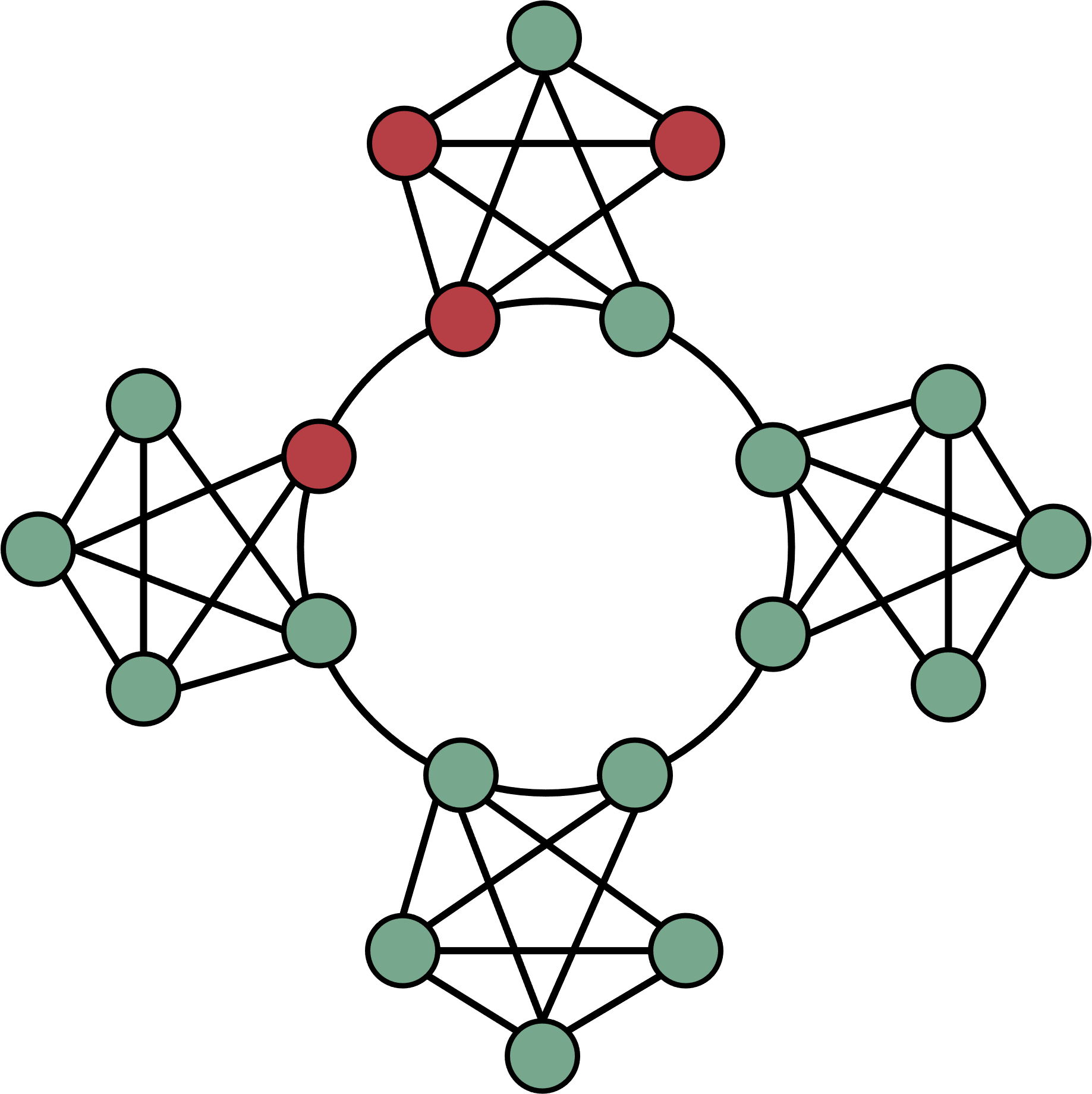
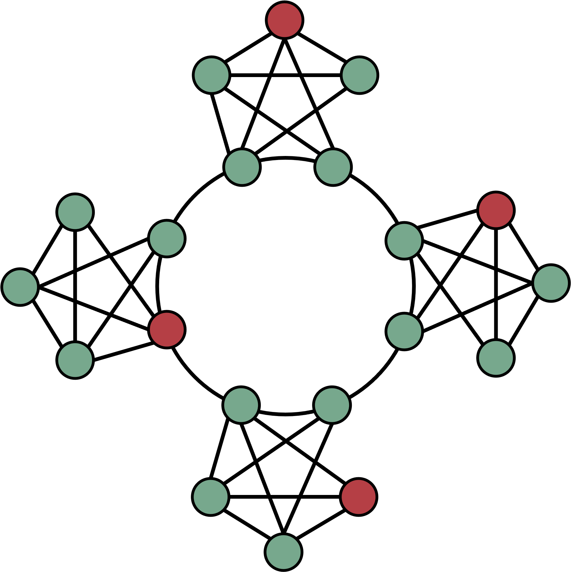
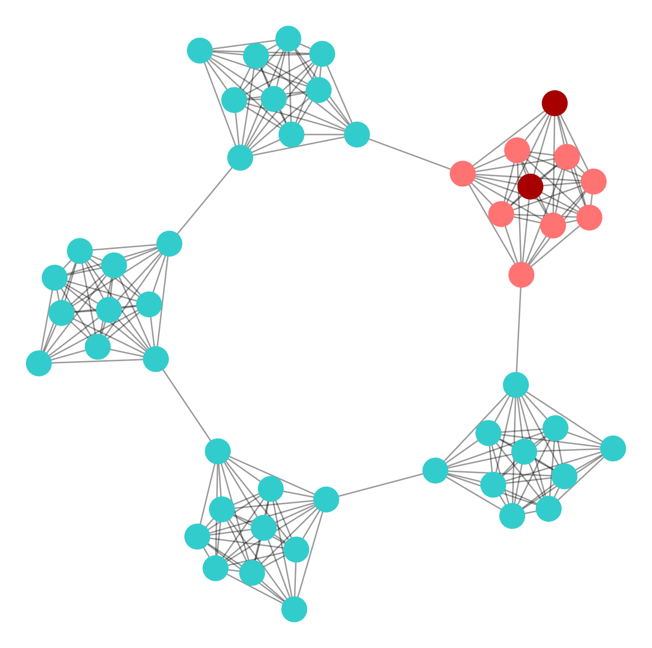
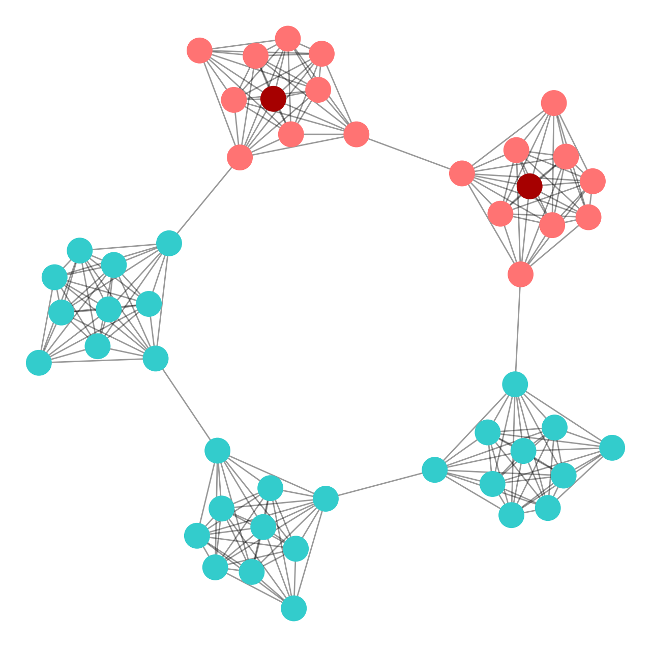
To empower GNNs with being position-aware, recently, You et al.  [2] proposed position-aware graph neural networks (P-GNNs) by setting some nodes within the graph as anchors. Thereby, other nodes can know their relative distances by comparing their distances to anchors [2]. However, P-GNNs select anchors in a random fashion [2]. When the anchors are ill-selected, two issues arise: 1) Anchors are not evenly distributed within the graph. In P-GNNs, nodes learn their feature vectors via aggregating the representations of different anchors, and anchors extract features via aggregating information of their neighbors. Thus, if the anchors concentrate in a small subgraph (see the left of Figure 1), anchors cannot extract comprehensive information of a graph, leading to the poor representations of nodes far away from the anchors. 2) Anchors locate on symmetric nodes. Given the condition that all the nodes have the same features, two nodes are of symmetry if their learned representations are the same via message passing and aggregating. That is, the two subgraphs around the two nodes are isomorphic. If two anchors are symmetric, the distances from two symmetric nodes to the two anchors will be the same, causing position-unawareness. We will explain in more detail later in section IV.

To address the drawbacks due to random anchor selection mentioned above, we propose Position-Sensing Graph Neural Networks (PSGNNs). Instead of selecting anchors arbitrarily, the PSGNN contains a learnable anchor-selection component, enabling the network to choose anchors in a back-propagatable approach. Theoretically, we show selecting optimal anchors is equivalent to an NP-complete problem, leading to the impracticability of choosing optimal anchors with an efficient deterministic algorithm. Thus, selecting anchors through heuristics approaches like learning is inevitable. Practically, PSGNNs exhibit substantial improvement over a range of existing competitive GNNs on many graph datasets. Subsequent analysis discovers that PSGNNs select well-distributed and asymmetric anchors (see the right one in Figure 1). Furthermore, the performance of the PSGNN steadily grows as the graph size enlarges, reflecting its desirable scalability.

We summarize our contributions as follows:

1. We show the NP-complete hardship of selecting both well distributed and asymmetric anchors.

2. We propose PSGNNs that can learn to select ideal anchors in a back-propagatable fashion, outperforming various existing state-of-the-art models.

3. PSGNNs also reveal desirable scalability, learning relative positions between nodes well on giant graphs.

II Related Work

Existing GNN models originate from spectrum-based graph convolutional networks, although their current forms may seem to be very different from spectrum-based models [6]. Spectrum-based GNNs map input graphs to spectrum representations, indicating the degree of diffusion [7].

Original spectrum-based GNNs directly utilize Laplacian transformation [8] and the convolution theorem [9] to conduct convolutional operations on graphs [10]. To reduce the computational cost of Laplacian transformation, the Chebyshev approximation has been applied to address the high computational-cost operations [11]. Using the first two terms of the Chebyshev polynomials, Kipf et al. [12] proposed graph convolutional networks (GCNs). Following GCNs, various other GNNs have been conceived, such as graph attention networks (GATs) [13], graph sampling $\&$ aggregate (GraphSAGE) [14], and graph isomorphism networks (GIN) [15]. On the other hand, a range of network embeddings methods have also been presented, such as DeepWalk [16], LINE [17], and node2vec [18].

All the mentioned approaches follow the message passing and aggregating paradigm. GATs assign different weights to the messages received from distinct neighbors [13]. For GraphSAGE, a node receives messages from a sampled set of neighbors [14], instead of collecting embeddings from all the neighbors, and graph isomorphism networks (GINs) are inspired by the graph isomorphism problem to build GNNs that have the equivalent capability with the Weisfeiler-Lehman (WL) test proposed in the graph theory community [15].

Despite the improved performance, GNNs based on message passing and aggregating suffer from the over-smoothing problem [19] i.e., as the number of network layers increases, the performance of GNNs decreases. To address over-smoothing, Li et al.  [20] proposed deep GCNs using residual connections to improve the efficiency of back-propagation.

To study the theoretical power of GNNs, Xu et al.  [15] state that the capability of existing GNNs in differentiating two isomorphic graphs does not exceed the 1-Weisfeiler-Lehman (1-WL) test [21]. In other words, without assigning different nodes with distinct features, many existing GNNs, e.g. GCNs and GraphSage, embed nodes that are in symmetric locations into the same embeddings.

Hence, although the above GNNs demonstrate excellent performance in some tasks like node classification, the node embeddings learned by these GNNs do not contain relative positions for two nodes in symmetric locations. To enable position-awareness in GNNs, You et al.  [2] presented position-aware graph neural networks (P-GNNs) and are the most relevant model to our proposed model. P-GNNs set some nodes within the graph as anchors so that other nodes can know their relative distances from the designated anchors.

You et al.  [2] also introduced the identity-aware GNN (ID-GNN) that can extend the expressing capability of GNNs beyond the 1-WL test. However, the work focuses on empowering different nodes with distinct representations instead of making GNNs position-aware. That is, the embeddings of two nodes learned by ID-GNNs do not preserve their distance information, whereas this information is retained to have low distortion by P-GNNs.

Regardless of the possibility of learning relative distances between graph nodes, P-GNNs select anchors randomly. This paper shows that the random selection of anchors leads to performance compromise and position unawareness. Moreover, we present a solution model: Position-Sensing Graph Neural Networks, to address the problems of random anchor selection.

III Preliminaries

Graph Neural Networks

Graph neural networks (GNNs) are able to learn the lower-dimensional embeddings of nodes or graphs [22]. In general, GNNs apply a neighborhood aggregation strategy [23] iteratively. The strategy consists of two steps: first, every node aggregates information from its neighbors; second, each node combines the aggregated information with its own information [15]. We write the two steps as the following two formulas:

$$a_{v}^{(k)}=\text{Aggregate}^{(k)}(\{h_{u}^{(k-1)}|u\in\text{Neighbor}(v)\}),$$

$$h_{v}^{(k)}=\text{Combine}^{(k)}(h_{v}^{(k-1)},a_{v}).$$

In the above equations, $a_{v}$ is the function to aggregate all the information of the neighbor nodes around node $v$. Moreover, $h_{v}^{(k)}$ stands for the embedding of node $v$ at layer $k$. Different GNNs employ distinct aggregation and combination strategies. The iterations continue for $k$ steps. The number $k$ is the layer number of a GNN. To reduce verbosity, we refer to the GNNs following the mentioned pattern of aggregating and combining simply as standard GNNs.

(a) Without anchors

(b) With an anchor

Figure 2: Illustration of symmetric node positions. The two blue nodes are in symmetric locations within each graph. The dotted blue node represents an anchor.

IV Relative Positions Learning

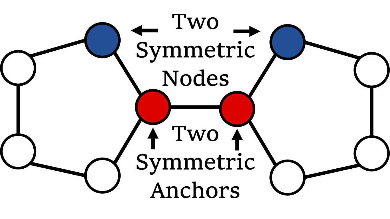
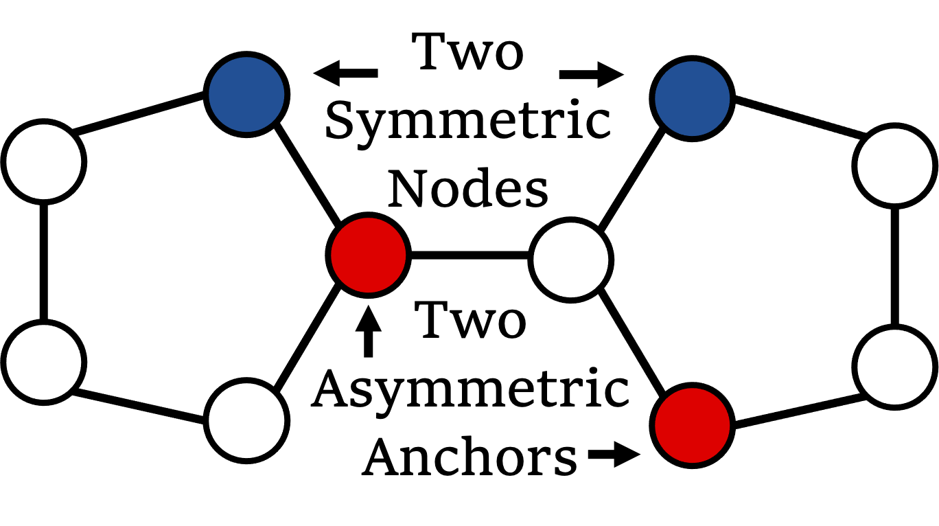
To reiterate, P-GNNs [2] aim to enable position-awareness during GNNs learning embeddings via message passing and aggregating. For example, as Figure 2 illustrates, the two dotted nodes will be assigned with the same embeddings by a standard GNN, but their distances to the dotted node are different. In P-GNNs, these special nodes are called anchors [2]. Therefore, using the distances from every node to the anchors, P-GNNs will know the relative positions among nodes.

Although P-GNNs have been equipped with position-awareness of nodes, P-GNNs select anchor sets in a random fashion. Such randomness leads to two problems.

First, the neighbors of randomly selected anchors may not cover all the nodes within a graph. Here, we say if a node is a $k$-hop neighbor of an anchor, where $k$ is the number of layers for a GNN to learn anchor embeddings, we then say the anchor covers the node. We consider that anchors are better if they can cover every node within the graph because we assume such anchors together contain more knowledge about the features and structures of the graph than anchors covering only a subset of graph nodes. For example, Figure 3 exhibits the anchors’ cases covering more and fewer nodes. We consider the coverage of anchors being non-overlapped is better than being overlapped since the mutually non-overlapping anchor coverage leads to different anchors containing information of distinct nodes. Thus, the features of two anchors are more likely to be orthogonal.

Second, as Liu et al.  [24] have also pointed out; if anchors locate on symmetric nodes, symmetric nodes will have the same distances to the anchors. Consequently, P-GNNs become position-unaware for some graph nodes. For example, as 3(a) illustrates, two anchors (the red nodes) are located on symmetric locations. As a result, the two symmetric nodes will then have the same embeddings learned from a P-GNN since the two distances to the two anchors, from the two nodes are the same. The symmetric anchors then cause the embeddings of the two nodes not to be differentiable, making P-GNNs fail to capture the relative positions between them.

Our proposed approach is motivated by these two limitations. In sum, both problems root in flawed anchor selection. One intuitive idea can be to devise deterministic algorithms for choosing anchors. However, in the following, we will show that selecting anchors is not a trivial problem. Specifically, to address the first problem, i.e., to select anchors covering the entire graph, we show this is equivalent to an NP-complete problem.

(a) Non-Overlapping Coverage

(b) Overlapping Coverage

Figure 3: Illustration of the covered nodes (yellow nodes) of anchors (red nodes).

Proposition 1.

Selecting the smallest collection of anchors that cover the entire graph is NP-complete.

Proof.

Suppose the GNN that is to learn the embeddings of the anchors has $k$ layers. Consequently, each anchor has access to its neighbors with a maximum distance $k$ to the anchor. We desire that the nodes within the graph are contained within the $k$-hop of the anchors’ neighbors.

NP: Given a collection of anchors, it requires the complexity of $O(\mathcal{N})$ to check whether the anchors can cover the entire graph within $k$ hops. Therefore, the problem is in NP.

Reduction: We show the dominant set problem, known to be NP-complete [25], can be reduced to the problem of selecting anchors that extract information from the entire graph. Given a graph within the dominant set problem. We represent the graph as adjacency matrix $\mathbf{A}$. Afterward, we construct a new matrix $\mathbf{A}_{k}$ such that entry $(i,j)$ is $1$ iff the distance between nodes $i$ and $j$ is less than $k$. Such matrix $\mathbf{A}_{k}$ can be obtained by iteratively multiplying adjacency matrix $\mathbf{A}$ with itself for $k$ times. Next, we obtain the graph corresponding to the adjacency matrix $\mathbf{A}_{k}$. Then, the problem of discovering the dominant set of $\mathbf{A}_{k}$ is equivalent to selecting the smallest collection of anchors whose distances to every node within a graph is less than $k$. This concludes the reduction, indicating the hardship bounded by NP-completeness.

Thus, selecting a set of anchors that can cover the entire graph is of NP-completeness. ∎

V Our Approaches

Input: Graph $G=(\mathcal{V},\mathcal{E})$; Node input features $\{\mathbf{x}_{v}\}$

Output: Position-Aware Node embeddings

for $l=1,...,L$ do

       // Anchor-selection component.

•  

  Extract node features via message passing and aggregating using a GNN;

Transform node features to the likelihoods of   serving as anchors;

 

Acquire vector o with each entry as a likelihood;

 

$\epsilon\sim\mathcal{N}(\mathbf{0},\mathbf{I})$;

 

Update $\mathbf{o}$ by adding it with $\alpha\cdot\epsilon$;

Select the nodes corresponding to the top $k$ maximum dimensions in o as the collection   of anchors $A$;

       for $a\in A$ do

             Learning the embedding for anchor $a$ via message passing and aggregating;

            

       end for

      // Learning position-aware node representations.

       for $v\in V$ do

             for $a\in A$ do

•              

  Obtain distance $d_{v,a}$ from $v$ to $a$;

             

Transform distance $d_{v,a}$ via FC layer;

             

Obtain the embedding of anchor $a$ as $e_{a}$;

Obtain the message to node $v$ as the dot               product between $d_{v,a}$ and $e_{a}$ as $m$;

Concatenate the self embedding of node $v$               and the message embedding $m$ as $c_{v,m}$;

Transform $c_{v,m}$ as the new embedding of               node $v$ via FC layer;

                  

             end for

            

       end for

      

end for

Algorithm 1 Procedures of the PSGNN for an epoch.

V-A Problem Formulation

We aim to create a neural network that can learn to pick the representative anchors. Features of these anchors comprise information of the entire graph. Mathematically, we can express this model $s_{\phi}$ for selecting anchors as:

$$s_{\phi}:(\mathcal{V},\mathcal{E})\rightarrow\{v_{i}\}_{i=1}^{M},$$ (1)

where $\phi$ denotes the parameters of model $s$, $\{(\mathcal{V},\mathcal{E})_{i}\}_{i=1}^{N}$ is a set of graphs, $\mathcal{V}$ and $E$ correspond to vertices and edges, and $\{v_{i}\}_{i=1}^{M}$ is the $M$ most optimum anchors to pick.

V-B Position-Sensing Graph Neural Network

We desire to devise a learning model that can achieve the anchor selection process of Equation 1 in a differentiable fashion. To this end, we design the anchor-selection model as a composition of a GNN $\mathbf{g}$ and a following transformation layer $\mathbf{f}$, expressed as:

$$s_{\phi}\big{[}(\mathcal{V},\mathcal{E})\big{]}=\mathbf{f}\circ\mathbf{g}\big{[}(\mathcal{V},\mathcal{E})\big{]}=\mathbf{o}.$$ (2)

The $\mathbf{g}$ component can be any GNN models such as GCN, GAT, and GIN. The transforming layer $\mathbf{f}$ requires the output values to be within the range between 0 and 1. In our implementation, we use a fully-connected layer, followed by a $\ell_{2}$-normalization layer. However, other normalization layers can also be used.

To overcome the non-differentiability in Equation 1, instead of directly selecting anchors, we output the likelihood of every node being chosen as an anchor. Intuitively, GNN $\mathbf{g}$ extracts features for every node, followed by FC layer $\mathbf{f}$ to transform the extracted node representations into the likelihoods. Consequently, $s_{\phi}\big{[}(\mathcal{V},\mathcal{E})\big{]}$ outputs a vector with dimension $N$, where every entry in the vector represents the likelihood for the corresponding node. We denote this output vector as $\mathbf{o}$. The mapping from the entry index to the node needs to be predefined. In our case, we assign every node a unique index ranging from $1$ to $N$ inclusively, and we map the entry index to the node with the same index. To illustrate, suppose there are $10$ nodes within a graph. Then, the IDs of the nodes will range from $1$ to $10$ inclusively.

Next, we need to sample $k$ anchors from the $N$ nodes based on likelihood vector $\mathbf{o}$. We need to trade-off between exploration and exploitation of selecting anchors. Exploration is to select the anchors that have not been selected before, and exploitation is to stick using the previously-selected anchors that lead to low loss values. To this end, we add a randomly generated noise $\epsilon\sim\mathcal{N}(\mathbf{0},\mathbf{I})\in\mathcal{R}^{N}$ to the likelihood vector $\mathbf{o}$:

$$\mathbf{o}+\alpha\cdot\epsilon,$$ (3)

where $\alpha$ is a hyperparameter controlling the trade-off. Larger $\alpha$ indicates more randomness.

To illustrate, if we are to choose $M=2$ anchors, then given the assumption where after adding noise $\epsilon$, the $2$-nd and $4$-th dimensions are of the top-$2$ maximum within the output vector $\mathbf{o}$ of anchor-selection model $s$, the nodes with IDs $2$ and $4$ will be selected as the anchors.

Once we have determined the indices of the anchors, we need to assign every node with an anchor. We denote this function as $A_{v}=A(v)$, where $v$ is a node and $A_{v}$ represents the anchor of node $v$. Following [2], for each node, we pick the anchor that has the minimum distance to the node compared with the other anchors.

Next, we update node $v$’s embedding based on its own features, the message from its anchor $A_{v}$ to the anchor. We first fuse the information of distance and the anchor’s embedding via conducting a dot product of them. In formula, $m=e_{a}\cdot e_{v}$, where $m$ stands for the message from the anchor to node $v$, and $e_{a}$ and $e_{v}$ represent the embedding and anchor $a$ and node $v$. Then, we concatenate the message from the anchor and the node’s own embedding, followed by conducting transformation of this concatenated result. This transformed result then acts as the new embedding of the node.

The detailed algorithmic procedures of the PSGNN are provided in algorithm 1.

V-C Working Mechanisms

Our PSGNN learns to select anchors in a trial-and-error approach. With back-propagation, it can choose increasingly more appropriate anchors for downstream tasks. We show the intuitive working mechanisms here.

Suppose there is only one anchor, and the node with ID 3 (denote as node 3 for brevity) is the ideal anchor. However, our anchor-selection model $\mathbf{s}$ wrongly chooses node 4 as the anchor. That is, the likelihood in the 4-th entry of output vector $\mathbf{o}$ is larger than that of the 3-th entry, i.e., $\mathbf{o}_{4}>\mathbf{o}_{3}$. Due to selecting an sub-optimal anchor, the loss value is not minimum.

Since PSGNN contains randomness in selecting anchors, given enough times of sampling, node 3 will be selected as an anchor at some time. As node 3 is more appropriate to be an anchor than node 4, the loss value is likely to be smaller. As a result, back-propagation will increase $\mathbf{o}_{3}$. Next time, $\mathbf{o}_{3}$ will have higher chance in selecting node 3.

TABLE I: AUC results of comparing PSGNNs against existing competitive baselines on various datasets for pairwise node classification and link prediction tasks. Best results are highlighted with bold face and the red color.

(a) Pairwise node classification.

	Communities	Email	Protein
GCN	$0.513\pm 0.025$	$0.502\pm 0.014$	$0.508\pm 0.012$
GraphSAGE	$0.521\pm 0.013$	$0.519\pm 0.086$	$0.504\pm 0.007$
GAT	$0.607\pm 0.019$	$0.509\pm 0.017$	$0.518\pm 0.017$
GIN	$0.609\pm 0.101$	$0.532\pm 0.018$	$0.524\pm 0.009$
Position-Aware Methods
PGNN	$0.912\pm 0.071$	$0.563\pm 0.012$	$0.502\pm 0.023$
PSGNN (Ours)	$\mathbf{0.978\pm 0.035}$	$\mathbf{0.736\pm 0.017}$	$\mathbf{0.533\pm 0.018}$

(b) Link prediction.

	Communities	Grids	Bio-Modules
GCN	$0.423\pm 0.027$	$0.509\pm 0.012$	$0.529\pm 0.012$
GraphSAGE	$0.502\pm 0.011$	$0.515\pm 0.048$	$0.527\pm 0.009$
GAT	$0.565\pm 0.020$	$0.522\pm 0.042$	$0.533\pm 0.005$
GIN	$0.509\pm 0.034$	$0.547\pm 0.028$	$0.510\pm 0.010$
Position-Aware Methods
PGNN	$0.927\pm 0.023$	$0.765\pm 0.062$	$0.913\pm 0.015$
PSGNN (Ours)	$\mathbf{0.954\pm 0.032}$	$\mathbf{0.942\pm 0.044}$	$\mathbf{0.989\pm 0.001}$

TABLE II: Scalability analysis of PSGNNs against existing competitive GNNs. Standard deviations are given. Best results are highlighted with bold face and the red color.

(a) AUC scores for pairwise node classification on communities with different numbers and sizes. C stands for the number of communities and S represents the community size.

Methods	C2; S8	C2; S32	C2; S64	C32; S8	C32; S32	C32; S64	C64; S8	C64; S32	C64; S64
GCN	$0.473\pm 0.101$	$0.504\pm 0.042$	$0.546\pm 0.028$	$0.503\pm 0.036$	$0.521\pm 0.023$	$0.538\pm 0.004$	$0.505\pm 0.012$	$0.524\pm 0.006$	$0.527\pm 0.012$
GraphSAGE	$0.584\pm 0.137$	$0.492\pm 0.014$	$0.505\pm 0.007$	$0.481\pm 0.032$	$0.490\pm 0.001$	$0.506\pm 0.002$	$0.485\pm 0.007$	$0.493\pm 0.001$	$0.495\pm 0.008$
GAT	$0.510\pm 0.113$	$0.493\pm 0.026$	$0.557\pm 0.022$	$0.514\pm 0.025$	$0.516\pm 0.001$	$0.517\pm 0.005$	$0.483\pm 0.032$	$0.515\pm 0.009$	$0.512\pm 0.003$
GIN	$0.424\pm 0.195$	$0.491\pm 0.023$	$0.507\pm 0.012$	$0.463\pm 0.021$	$0.492\pm 0.009$	$0.503\pm 0.006$	$0.462\pm 0.035$	$0.501\pm 0.007$	$0.503\pm 0.009$
Position-Aware Methods
P-GNN	$0.756\pm 0.172$	$0.773\pm 0.041$	$0.770\pm 0.063$	$0.875\pm 0.121$	$0.912\pm 0.074$	$0.856\pm 0.113$	$0.882\pm 0.071$	$0.925\pm 0.078$	$0.892\pm 0.093$
PSGNN	$\mathbf{0.842\pm 0.081}$	$\mathbf{0.843\pm 0.024}$	$\mathbf{0.857\pm 0.002}$	$\mathbf{0.981\pm 0.007}$	$\mathbf{0.983\pm 0.008}$	$\mathbf{0.992\pm 0.003}$	$\mathbf{0.994\pm 0.004}$	$\mathbf{0.995\pm 0.003}$	$\mathbf{0.997\pm 0.007}$

(b) AUC scores for link prediction of the grid dataset with various sizes. Standard deviations are given. Bold texts represent the best performance. The splitting line in the middle divides position-aware methods from position-unaware methods.

Methods	$16\times 16$	$20\times 20$	$24\times 24$	$28\times 28$	$32\times 32$	$36\times 36$	$40\times 40$	$44\times 44$	$48\times 48$
GCN	$0.482\pm 0.003$	$0.525\pm 0.031$	$0.492\pm 0.014$	$0.497\pm 0.013$	$0.519\pm 0.002$	$0.493\pm 0.024$	$0.506\pm 0.013$	$0.511\pm 0.018$	$0.513\pm 0.025$
GraphSAGE	$0.563\pm 0.042$	$0.586\pm 0.073$	$0.612\pm 0.082$	$0.556\pm 0.024$	$0.611\pm 0.030$	$0.624\pm 0.007$	$0.682\pm 0.046$	$0.633\pm 0.042$	$0.637\pm 0.031$
GAT	$0.612\pm 0.065$	$0.604\pm 0.058$	$0.642\pm 0.013$	$0.605\pm 0.002$	$0.657\pm 0.031$	$0.613\pm 0.027$	$0.592\pm 0.025$	$0.582\pm 0.047$	$0.633\pm 0.032$
GIN	$0.461\pm 0.015$	$0.503\pm 0.027$	$0.413\pm 0.031$	$0.448\pm 0.021$	$0.480\pm 0.002$	$0.453\pm 0.021$	$0.423\pm 0.006$	$0.467\pm 0.023$	$0.441\pm 0.008$
Position-Aware Methods
P-GNN	$0.653\pm 0.162$	$0.628\pm 0.072$	$0.643\pm 0.054$	$0.526\pm 0.022$	$0.591\pm 0.038$	$0.623\pm 0.065$	$0.657\pm 0.089$	$0.591\pm 0.023$	$0.565\pm 0.040$
PSGNN	$\mathbf{0.901\pm 0.023}$	$\mathbf{0.924\pm 0.021}$	$\mathbf{0.945\pm 0.019}$	$\mathbf{0.949\pm 0.024}$	$\mathbf{0.952\pm 0.013}$	$\mathbf{0.955\pm 0.003}$	$\mathbf{0.956\pm 0.032}$	$\mathbf{0.961\pm 0.008}$	$\mathbf{0.963\pm 0.007}$

TABLE III: The complexity of selecting anchors with rule-based heuristics and learning methods, as well as their AUC results on communities for pairwise node classification (Pair Node Cls) and on grids for link prediction (Link Pred). The best results are highlighted in bold face with the red color.

		Tasks
Methods	Complexity	Pair Node Cls	Link Pred
Degree	$\mathbf{O\big{(}|\mathcal{V}|\big{)}}$	$0.930\pm 0.012$	$0.830\pm 0.023$
Betweenness	$O\big{(}|\mathcal{V}|^{3}\big{)}$	$0.944\pm 0.007$	$0.756\pm 0.031$
Harmonic	$O\big{(}|\mathcal{V}|^{3}\big{)}$	$0.958\pm 0.018$	$0.733\pm 0.032$
Closeness	$O\big{(}|\mathcal{V}|^{3}\big{)}$	$0.978\pm 0.007$	$0.765\pm 0.012$
Load	$O\big{(}|\mathcal{V}|^{3}\big{)}$	$0.974\pm 0.012$	$0.778\pm 0.034$
P-GNN	$O\big{(}|\mathcal{E}|+|\mathcal{V}|\log|\mathcal{V}|\big{)}$	$0.892\pm 0.093$	$0.565\pm 0.040$
PSGNN	$\mathbf{O\big{(}|\mathcal{V}|\big{)}}$	$\mathbf{0.997\pm 0.007}$	$\mathbf{0.963\pm 0.007}$

VI Experiment

VI-A Datasets and Tasks

We experiment on both synthetic and real-world graph datasets. We employ the following three datasets for the link prediction task.

Communities. A synthetic connected caveman graph with 20 communities, each community consisting of 20 nodes. Every pair of communities are mutually isomorphic.

Grid. A synthetic 2D grid graph of size $20\times 20$ (400 nodes) with all the nodes having the same feature.

Bio-Modules [26]. A gene regulatory network produced by simulated evolutionary processes. A link reflects two genes have mutual effects. Each node contains a two-dimensional one-hot vector, indicating the corresponding gene is either in activation or repression.

Cora, CiteSeer and PubMed [13]. Three real-world citation networks consisting of 2708, 3327, and 19717 nodes, respectively, with each node representing an artificial intelligence article. Every dimension of the node’s feature vector is a binary value, indicating the existence of a word.

We also perform the pairwise node classification task on the following three datasets.

• Communities. The structure is the same as described above. Each node’s label corresponds to the community it is belonging.

• Emails. Seven real-world email communication networks from SNAP [27]. Each graph comprises six communities. Every node has a label indicating the community to which it belongs.

• Protein. 1113 real-world protein graphs from [28]. Each node contains a 29-dimensional feature vector and is labeled with a functional role of the protein.

VI-B Experimental Setups

Node Features. For synthetic datasets, all the node features of a graph are the same. Consequently, GNNs can only utilize relative positions among nodes to conduct pairwise node classification and link prediction, reflecting the GNN’s position awareness. However, in practice, nodes can have meaningful features. Thus, for real-world citation networks, i.e., Cora, CiteSeer, and PubMed, we include every node with semantic features. However, this leads to position-awareness being not the single clue for the task. This semantic information can also disclose the affinity between two nodes.

Train/Valid/Test Split. We follow the setting from [2] and use 80% existing links and the same number of non-existing ones for training, as well as the remaining two sets of 10% links for validating and testing, respectively. We report the performance on the test set using the model, which achieves the highest accuracy on the validation set. For a task on a specific dataset, we independently train ten models with different random seeds and train/validation splits, and report the average performance and the standard deviation.

Loss Functions. Binary cross-entropy [29] is employed as the loss function to train the PSGNN.

Baselines. We compare the PSGNN against existing popular GNN models. For a fair comparison, all the models are set to have the same hyperparameters. Specifically, we employ the Adam optimizer, with the learning rate set as $1\times 10^{-3}$. We set the number of anchors to be $\log N$, where $N$ is the number of nodes within a graph. $\alpha$ in Equation 3 is set to be $0.5$. All the GNN models contain three layers. The implementation is based on the PyTorch framework trained with two NVIDIA 2080-Ti GPUs.

VI-C Comparison Against State-of-the-Art

Table I demonstrate comparing the performance of PSGNNs with existing competitive GNN models on the above datasets for pairwise node classification and link prediction. We discover that since GCNs cannot be aware of node positions, they reveal nearly random performance on both tasks’ datasets. Other position-unaware models show negligible improvements over GCNs. In contrast, P-GNNs exhibits breakthrough improvements on some datasets. Moreover, our PSGNNs further substantially enhance the performance over P-GNNs, achieving the best AUC scores on all the datasets of both tasks. In particular, the average increase on the email and grid datasets reaches more than 27%, and the AUC scores for all the synthetic datasets surpass 0.9. These performances indicate the effectiveness of our PSGNNs.

On the other hand, PGNNs first select different anchor sets, then within each anchor set, a node chooses the anchor as the one having the minimum distance to the node within the set. In contrast, instead of selecting anchors from the pre-selected anchor sets as P-GNNs, PSGNNs directly select anchors, leading to a lower computational complexity than that of P-GNNs. Specifically, during each node learning its embedding from an anchor, P-GNN requires $O(M\cdot(|\mathcal{E}|+|\mathcal{V}|\log|\mathcal{V}|))$, where $M$ is the cardinality of an anchor set, whereas PSGNN demands $O((|\mathcal{E}|+|\mathcal{V}|\log|\mathcal{V}|))$

Figure 4: The AUC results for comparing the performance of link prediction between P-GNNs and PSGNNs on three real-world citation networks.

VI-D Analysis on Scalability

We also study the scalability of PSGNNs and other GNNs. That is, how the performance changes as the graph size increases. The results are reported in II(b). We discover that for the GNNs to be position-unaware, their performances are similar to randomness, regardless of the graph size.

In contrast, for pairwise node classification on communities, both GNNs can learn the relative positions among nodes, i.e., PGNNs and PSGNNs, show increasing AUC scores as the graph size increases. Besides, PSGNNs demonstrate better performance for all the graph sizes over PGNNs and better stability. Moreover, the PSGNNs performance steadily grows, whereas the trend of PGNNs depicts fluctuations. On the other hand, for link prediction on grids, the PGNNs scalability is limited, revealing a decreasing tendency with the increasing graph size. On the contrary, PSGNNs still maintain a positive correlation between AUC and the graph sizes, indicating their general flexibility on different datasets and tasks.

VI-E Networks with Abundant Features

The design concept of position-aware GNNs is to capture the pairwise distance among nodes with no or scarce features. These situations force GNNs to merely utilize the structural information of a graph to infer the pairwise distances. The node having inadequate features is a common scenario in real-world applications since features can be hard to collect due to privacy protection and other reasons.

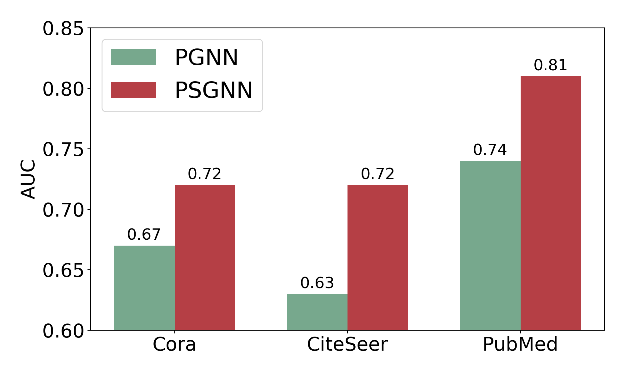
However, for other graphs such as citation networks, nodes can have rich publicly available features. These graphs are not targeted applications of PGNNs and PSGNNs since pairwise distances between nodes can be implicitly inferred from the feature affinity. Thus, it is unfair to compare performance between position-aware GNNs and other GNNs. We therefore only compare PSGNNs against PGNNs on three benchmark citation networks, i.e., Cora, CiteSeer, and PubMed, and report the results in Figure 4. We see PSGNNs consistently outperform P-GNNs on all three datasets. Furthermore, PSGNNs also demonstrate better scalability than PGNNs. Specifically, the performance of PGNNs firmly increases as the size of the graph grows, whereas the trend of PSGNNs indicates fluctuation.

VI-F Necessity of Learning Anchors

We have described before that selecting proper anchors is of NP-completeness. Although it is impractical to discover an optimal solution toward an NP-complete problem, rule-based heuristic algorithms can lead to sub-optimal approaches. For example, [24] proposes to select the nodes with the most significant degrees as anchors. Nonetheless, although these rule-based heuristic methods have lower computational complexity than the exponential level, the run-time is still higher than the linear cost of our anchor-learning component (see Table III for the comparison in detail). Specifically, PSGNN uses a standard GNN to assign the likelihoods of being selected as anchors, where aggregating and messaging takes $O(|\mathcal{V}|)$. Furthermore, selecting the top-$k$ anchors can be done in linear time. Therefore, PSGNN takes $O(|\mathcal{V}|)$ to select anchors. Thus, the rule-based approaches have more insufficient scalability than PSGNNs. Furthermore, we also compare the performance of learning anchors against rule-based selections on both pairwise node classification and link prediction tasks. The datasets for the two tasks are a connected Caveman graph with 64 communities, each having 64 nodes, and a $48\times 48$ grid network, respectively. We observe that the PSGNN consistently outperforms the rule-based heuristic methods while it enjoys a lower computational complexity.

VII Conclusion

Despite increasing attention in GNNs, relatively little work focuses on predicting the pairwise relationships among graph nodes. Our proposed position-sensing graph neural networks (PSGNNs) can extract relative positional information among graph nodes, substantially improving pairwise node classification and link prediction over a variety of baseline GNNs. Our PSGNN also exhibit great scalability. Apart from practical contributions, theoretically, this paper brings NP-completeness theory in analyzing the complexity of GNN algorithms.

Acknowledgments: This work was partly supported by the National Research Foundation of Korea(NRF) grant funded by the Korea government(MSIT) (No. 2020R1F1A1061667).

References

- [1] Zonghan Wu, Shirui Pan, Fengwen Chen, Guodong Long, Chengqi Zhang, and S Yu Philip, “A comprehensive survey on graph neural networks,” IEEE TNNLS, 2020.
- [2] Jiaxuan You, Rex Ying, and Jure Leskovec, “Position-aware graph neural networks,” in ICML, 2019, pp. 7134–7143.
- [3] EL-MOUSSAOUI Mohamed, Tarik Agouti, Abdessadek Tikniouine, and Mohamed El Adnani, “A comprehensive literature review on community detection: Approaches and applications,” Procedia Computer Science, vol. 151, pp. 295–302, 2019.
- [4] Muhan Zhang and Yixin Chen, “Link prediction based on graph neural networks,” in Advances in Neural Information Processing Systems, 2018, pp. 5165–5175.
- [5] Nur Nasuha Daud, Siti Hafizah Ab Hamid, Muntadher Saadoon, Firdaus Sahran, and Nor Badrul Anuar, “Applications of link prediction in social networks: A review,” Journal of Network and Computer Applications, p. 102716, 2020.
- [6] Filippo Maria Bianchi, Daniele Grattarola, and Cesare Alippi, “Spectral clustering with graph neural networks for graph pooling,” ICML, 2020.
- [7] Joan Bruna, Wojciech Zaremba, Arthur Szlam, and Yann LeCun, “Spectral networks and locally connected networks on graphs,” ICLR, 2013.
- [8] Eduardo Pavez and Antonio Ortega, “Generalized laplacian precision matrix estimation for graph signal processing,” in 2016 IEEE International Conference on Acoustics, Speech and Signal Processing (ICASSP). IEEE, 2016, pp. 6350–6354.
- [9] Bingbing Xu, Huawei Shen, Qi Cao, Yunqi Qiu, and Xueqi Cheng, “Graph wavelet neural network,” in International Conference on Learning Representations, 2018.
- [10] Hermina Petric Maretic and Pascal Frossard, “Graph laplacian mixture model,” IEEE Transactions on Signal and Information Processing over Networks, vol. 6, pp. 261–270, 2020.
- [11] Michaël Defferrard, Xavier Bresson, and Pierre Vandergheynst, “Convolutional neural networks on graphs with fast localized spectral filtering,” in Advances in neural information processing systems, 2016, pp. 3844–3852.
- [12] Thomas N Kipf and Max Welling, “Semi-supervised classification with graph convolutional networks,” ICLR, 2016.
- [13] Petar Veličković, Guillem Cucurull, Arantxa Casanova, Adriana Romero, Pietro Lio, and Y Bengio, “Graph attention networks,” ICLR, 2017.
- [14] Will Hamilton, Zhitao Ying, and Jure Leskovec, “Inductive representation learning on large graphs,” in Advances in neural information processing systems, 2017, pp. 1024–1034.
- [15] Keyulu Xu, Weihua Hu, Jure Leskovec, and Stefanie Jegelka, “How powerful are graph neural networks?,” ICLR, 2018.
- [16] Bryan Perozzi, Rami Al-Rfou, and Steven Skiena, “Deepwalk: Online learning of social representations,” in Proceedings of the 20th ACM SIGKDD international conference on Knowledge discovery and data mining, 2014, pp. 701–710.
- [17] Jian Tang, Meng Qu, Mingzhe Wang, Ming Zhang, Jun Yan, and Qiaozhu Mei, “Line: Large-scale information network embedding,” in Proceedings of the 24th international conference on world wide web, 2015, pp. 1067–1077.
- [18] Aditya Grover and Jure Leskovec, “node2vec: Scalable feature learning for networks,” in Proceedings of the 22nd ACM SIGKDD international conference on Knowledge discovery and data mining, 2016, pp. 855–864.
- [19] Deli Chen, Yankai Lin, Wei Li, Peng Li, Jie Zhou, and Xu Sun, “Measuring and relieving the over-smoothing problem for graph neural networks from the topological view.,” in AAAI, 2020, pp. 3438–3445.
- [20] Guohao Li, Matthias Muller, Ali Thabet, and Bernard Ghanem, “Deepgcns: Can gcns go as deep as cnns?,” in Proceedings of the IEEE International Conference on Computer Vision, 2019, pp. 9267–9276.
- [21] Nino Shervashidze, Pascal Schweitzer, Erik Jan Van Leeuwen, Kurt Mehlhorn, and Karsten M Borgwardt, “Weisfeiler-lehman graph kernels.,” Journal of Machine Learning Research, vol. 12, no. 9, 2011.
- [22] Franco Scarselli, Marco Gori, Ah Chung Tsoi, Markus Hagenbuchner, and Gabriele Monfardini, “The graph neural network model,” IEEE Transactions on Neural Networks, vol. 20, no. 1, pp. 61–80, 2008.
- [23] Keyulu Xu, Chengtao Li, Yonglong Tian, Tomohiro Sonobe, Ken-ichi Kawarabayashi, and Stefanie Jegelka, “Representation learning on graphs with jumping knowledge networks,” in International Conference on Machine Learning, 2018, pp. 5453–5462.
- [24] Chao Liu, Xinchuan Li, Dongyang Zhao, Shaolong Guo, Xiaojun Kang, Lijun Dong, and Hong Yao, “Graph neural networks with information anchors for node representation learning,” Mobile Networks and Applications, pp. 1–14, 2020.
- [25] Ching-Hao Liu, Sheung-Hung Poon, and Jin-Yong Lin, “Independent dominating set problem revisited,” Theoretical Computer Science, vol. 562, pp. 1–22, 2015.
- [26] Carlos Espinosa-Soto and Andreas Wagner, “Specialization can drive the evolution of modularity,” PLoS Comp Bio, vol. 6, no. 3, pp. e1000719, 2010.
- [27] Jure Leskovec, Jon Kleinberg, and Christos Faloutsos, “Graph evolution: Densification and shrinking diameters,” ACM TKDD, vol. 1, no. 1, pp. 2–es, 2007.
- [28] Karsten M Borgwardt and Hans-Peter Kriegel, “Shortest-path kernels on graphs,” in ICDM. IEEE, 2005, pp. 8–pp.
- [29] Zhenyue Qin, Dongwoo Kim, and Tom Gedeon, “Rethinking softmax with cross-entropy: Neural network classifier as mutual information estimator,” arXiv preprint arXiv:1911.10688, 2019.