Distantly-Supervised Long-Tailed Relation Extraction Using Constraint Graphs

Abstract

Label noise and long-tailed distributions are two major challenges in distantly supervised relation extraction. Recent studies have shown great progress on denoising, but paid little attention to the problem of long-tailed relations. In this paper, we introduce a constraint graph to model the dependencies between relation labels. On top of that, we further propose a novel constraint graph-based relation extraction framework(CGRE) to handle the two challenges simultaneously. CGRE employs graph convolution networks to propagate information from data-rich relation nodes to data-poor relation nodes, and thus boosts the representation learning of long-tailed relations. To further improve the noise immunity, a constraint-aware attention module is designed in CGRE to integrate the constraint information. Extensive experimental results indicate that CGRE achieves significant improvements over the previous methods for both denoising and long-tailed relation extraction.

1 Introduction

Relation extraction (RE), which aims to extract the semantic relations between two entities from unstructured text, is crucial for many natural language processing applications, such as knowledge graph completion [1, 2], search engines [3, 4] and question answering [5, 6]. Although conventional supervised approaches have been extensively researched, they are still limited by the scarcity of manually annotated data. Distantly supervised relation extraction (DSRE) [7] is one of the most promising techniques to address this problem, because it can automatically generate large scale labeled data by aligning the entity pairs between text and knowledge bases (KBs). However, distant supervision suffers from two major challenges when used for RE.

The first challenge in DSRE is label noise, which is caused by the distant supervision assumption: if one entity pair has a relationship in existing KBs, then all sentences mentioning the entity pair express this relation. For example, due to the relational triple (Bill Gates, Founded, Microsoft), distant supervision will generate a noisy label Founded for the sentence ”Bill Gates speaks at a conference held by Microsoft”, although this sentence does not mention this relation at all.

In recent years, many efforts have been devoted to improving the robustness of RE models against label noise. The combination of multi-instance learning and attention mechanism is one of the most popular strategies to reduce the influence of label noise [8, 9, 10]. This strategy extracts relations of entity pairs from sentence bags, with the objective of alleviating the sentence-level label noise. In addition, some novel strategies, such as reinforcement learning [11, 12], adversarial training [13, 14, 15, 16] and deep clustering [17, 18] also show great potential for DSRE. However, these approaches are driven totally by the noisy labeling data, which may misguide the optimization of parameters and further hurt the reliability of models.

To address this problem, some researchers attempt to enrich the background knowledge of models by integrating external information. In general, the external information, e.g., entity descriptions [19, 20], entity types [21, 22, 23] and knowledge graphs [24, 20], will be encoded as vector form, and then integrated to DSRE models by simple concatenation or attention mechanism. Compared with the above implicit knowledge, constraint rules are explicit and direct information that can effectively enhance the discernment of models in noisy instances. For example, the relation for the sentence ”Bill Gates was 19 when he and Paul Allen started Microsoft” can not be Child_of, since its head/tail entity must be a Person, while Microsoft is an Organization. Here, we define (Person, Child_of, Person) as a constraint for Child_of. However, directly removing the constraint-violating sentences from a dataset would result in loss of significant useful information (as demonstrated in Sec. 3.6.2). Hence, we explore a soft way to integrate the constraint information by attention mechanism in this paper.

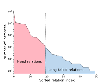
Figure 1: Instance number distribution of 52 positive relations in FB-NYT dataset. Relations with more than 100 instances are allocated to head relation, while the remaining relations belong to long-tailed relation. Note that the vertical axis uses a logarithmic scale.

The second challenge in DSRE is long-tailed relation extraction, however, which tends to be neglected as compared with the noisy labeling problem. In fact, real-world datasets of distant supervision always have a skewed distribution with a long tail, i.e., a small proportion of relations (a.k.a head relation) occupy most of the data, while most relations (a.k.a long-tailed relation) merely have a few training instances. As shown in Figure 1, more than 60% relations are long-tailed with fewer than 100 instances in the popular New York Times (FB-NYT) dataset [25]. Long-tailed relation extraction is important for knowledge graph construction and completion. Unfortunately, even the state-of-the-art DSRE models are not able to handle long-tailed relations well. Hence, how to train a balanced relation extractor from unbalanced data becomes a serious problem in relation extraction.

In general, long-tailed classfication tasks are addressed by re-sampling or re-weighting, nevertheless, long-tailed RE is special because the relation labels are semantically related rather than independent of each other. For example, if relation /location/country/capital holds, another relation /location/location/contains will holds as well. Therefore, a promising strategy for long-tailed RE is to mine latent relationships between relations by modeling the dependency paths. Once the dependency paths have been constructed, the relation labels are no longer independent of each other, and rich information can be propagated among the relations through these paths, which is crucial for the data-poor long-tailed relations. To accomplish this, [26] proposed the relation hierarchical tree, which connect different relation labels according to hierarchical information in the relation names. For instance, relation /people/person/nationality and relation /people/person/religion have the same parent node /people/person in the relation hierarchical tree. On account of its effectiveness, most of the previous long-tailed RE models [26, 27, 28, 29] rely on the relation hierarchical tree. However, relation hierarchical trees suffer from several limitations:

(1) the construction of the relation hierarchical trees requires the relation names in hierarchical format, which conflicts with many existing RE datasets, such as SemEval-2010 Task8 [30], TACRED [31], and FewRel [32, 33];

(2) the sparsity of the hierarchy tree hinders the representation learning of some extremely long-tailed relations;

(3) the optimization of parameters is purely driven by the noisy training data, lacking enough effective supervision signals. Specifically, the key goal of selective attention mechanism is to automatically recognize the noisy sentences and then reduce their weights, but this is not guaranteed. Although pre-trained knowledge graph embeddings were utilized by [27] to guide the learning of attention mechanism, they were simply used as initial embeddings of the relation labels.

To overcome the limitations of relation hierarchies, we explore the feasibility of utilizing another structure, constraint graph, to represent the intrinsic connection between relations. As shown in Figure 2, a constraint graph is a bipartite digraph [34], in which each directed edge connects a relation node to a type node or vice versa. As compared with entity-level knowledge graphs, constraint graphs provide more basic and general knowledge, more direct rule constraints, and a smaller vector space for knowledge mining and reasoning. Moreover, most knowledge bases (e.g. Freebase) preserve the entity type constraint information [35], which can be directly used for constraint graph construction. Even for datasets without relevant information, the constraint graph can be easily constructed according to the definition of each relation or the co-occurrence frequency of each relation with entity type pairs in the training set.

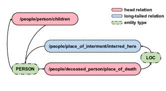
Figure 2: A subgraph of the constraint graph for FB-NYT. In this graph, the types of head and tail entities are respectively predecessors and successors of the corresponding relations.

In our observations, there are at least three kinds of information in constraint graphs that are beneficial to DSRE: (1) type information. As shown in many previous works [22, 36, 37, 38], entity types provide meaningful information for models to understand the entities, and play a crucial role in relation extraction; (2) constraint information. For example, it is obvious that the types of head and tail entities for relation /people/person/children are both Person. Such a constraint provides direct and effective prior information for DSRE models to recognize the noisy instances; (3) interactive information. As showed in Figure 2, relation nodes are connected indirectly through entity type nodes. Similar to the relation hierarchy-based methods, we can utilize message passing between nodes to transfer rich knowledge from head relations to long-tailed relations.

Based on the aforementioned motivations, we propose a novel constraint graph-based relation extraction framework (CGRE). Our framework consists of three main components: a sentence encoder used for encoding the corpus information, a graph encoder used for encoding the constraint graph information, and an attention module used for integrating different information from the two separate encoders. Specifically, we adopt graph convolution networks(GCNs) [39] as the graph encoder to extract interactive information from the constraint graph. Intuitively, the neighborhood integration mechanism of GCNs can efficiently improve the representation learning of long-tailed relations by propagating rich information from popular nodes to rare nodes. In addition, different from the plain selective attention [8], which is mainly dependent on the semantic similarity between sentences and relation labels, our constraint-aware attention combines both the semantic information and constraint information. In our approach, the attention score of each instance depends on not only its semantic similarity with the relation representations, but also its compatibility with the entity type constraints. We summarize our main contributions as follows:

• We explore a novel knowledge structure, constraint graph, to model the intrinsic dependencies between relation labels. Compared with the popular relation hierarchical trees, our constraint graph shows better universality, directness and effectiveness. We propose CGRE, a constraint graph-based DSRE framework, to simultaneously address the challenges of label noise and long-tailed distributions.

• We conduct large-scale experiments for performance comparison and ablation studies to demonstrate that CGRE is highly effective for both denoising and long-tailed RE.

• We make our pre-processed datasets and source code publicly available at https://github.com/tmliang/CGRE.

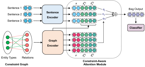
Figure 3: Overview of the proposed constraint graph-based framework. The sentence encoder aims to extract the representations for the sentences in a bag, while the graph encoder aims to extract the representations for the relations and the entity types from the constraint graph. In the constraint-aware attention module, selective attention is applied after concatenation operations to aggregate the three representations into a bag representation, based on which the classifier predicts the relations mentioned in the sentence bag.

2 Framework

Starting with notations and definitions, we will introduce the construction process for a raw constraint graph, and then detail each component of our framework. As illustrated in Figure 3, our framework consists of three key modules:

• Sentence Encoder. Given a sentence with two mentioned entities, the sentence encoder is adopted to derive a sentence representation.

• Graph Encoder. Given a raw constraint graph $\mathcal{G}$, we first transform it into an embedding matrix and then apply the graph encoder to extract the representations of relations and entity types.

• Constraint-Aware Attention. By combining outputs from the two seperate encoders, this module allocates an attention score for each instance in a bag, and then computes the bag representation.

2.1 Notations and Definitions

We define a constraint graph as a triple $\mathcal{G}=\{\mathcal{T},\mathcal{R},\mathcal{C}\}$, where $\mathcal{T}$, $\mathcal{R}$, $\mathcal{C}$ indicate the sets of entity types, relations, and constraints, respectively. Each constraint $(t_{r}^{e_{1}},r,t_{r}^{e_{2}})\in\mathcal{C}$ indicates that for relation $r$, the type of head entity can be $t_{r}^{e_{1}}\in\mathcal{T}$ and the type of tail entity can be $t_{r}^{e_{2}}\in\mathcal{T}$. Given a bag of sentences $\mathcal{B}=\{s_{1},\ldots,s_{n_{s}}\}$ and a corresponding entity pair $(e_{1},e_{2})$, the objective of distantly supervised relation extraction is to predict the relation $r_{i}$ for the entity pair $(e_{1},e_{2})$.

2.2 Constraint Graph Construction

Most knowledge bases provide the entity type constraint information. For example, in Freebase, these constraints are located in rdf-schema#domain and rdf-schema#range fields. However, the original constraints always involve thousands of entity types. To avoid over-parameterization, we merely use 18 coarse entity types defined in OntoNotes 5.0 [40], and then remove the constraints containing unrelated types. Finally, we can obtain a raw constraint graph $\mathcal{G}$ that consists of a relation set $\mathcal{R}$, a type set $\mathcal{T}$, and a constraint set $\mathcal{C}$. Note that we use a special type Others for the entities that do not belong to the 18 types, thus the size of $\mathcal{T}$ is 19. Specially, the negative category NA (i.e., no relations between the two entities) is connected to all types, since its head/tail entities could belong to any type. We emphasize that the constraint graph is specific to an entire dataset, rather than a bag in the dataset. That means one public constraint graph is shared by all the bags in the dataset. Furthermore, compared with the commonly used knowledge graph, the scale of a constraint graph is rather tiny. For example, there are merely 72 nodes (which is the sum of relation number and type number) and 164 edges in the constraint graph for the FB-NYT dataset.

2.3 Sentence Encoder

To encode the sentence information, we first adopt entity-aware word embeddings [41] to represent each word in a sentence, and then apply the Piecewise Convolutional Neural Network (PCNN) [42] to derive the sentence representation.

2.3.1 Input Layer

The input layer aims to maps words into a distributed embedding space to capture their semantic and syntactic information. Given a sentence $s=\{w_{1},\ldots,w_{l}\}$, we transform each word $w_{i}$ into a $d_{w}$-dimensional vector $\mathbf{w}_{i}$ by a pre-trained embedding matrix. Then following [41], we represent the target entities $e_{1}$ and $e_{2}$ by their word vectors $\mathbf{w}^{e_{1}}$ and $\mathbf{w}^{e_{2}}$. To incorporate the position information, we use two $d_{p}$-dimensional vectors $\mathbf{p}^{e_{1}}_{i}$ and $\mathbf{p}^{e_{2}}_{i}$ to embed the relative distances between $w_{i}$ and the target entities, as used in [42]. By concatenating, two types of word embeddings can be obtained as follows:

$$\mathbf{x}^{p}_{i} =[\mathbf{w}_{i};\mathbf{p}_{i}^{e_{1}};\mathbf{p}_{i}^{e_{2}}]\in\mathbb{R}^{d_{w}+2d_{p}},$$ (1)

$$\mathbf{x}^{e}_{i} =[\mathbf{w}_{i};\mathbf{w}^{e_{1}};\mathbf{w}^{e_{2}}]\in\mathbb{R}^{3d_{w}},$$

where $d_{w}$ and $d_{p}$ are both pre-defined hyper-parameters. Finally, we apply the entity-aware word embedding to represent each word $w_{i}$ as follows:

$$\mathbf{A}^{e}=\operatorname{sigmoid}\left(\lambda\cdot\left(\mathbf{W}_{e}\mathbf{X}^{e}+\mathbf{b}_{e}\right)\right),$$ (2)

$$\tilde{\mathbf{X}}^{p}=\operatorname{tanh}\left(\mathbf{W}_{p}\mathbf{X}^{p}+\mathbf{b}_{p}\right),$$

$$\mathbf{X}=\mathbf{A}^{e}\odot\mathbf{X}^{e}+\left(1-\mathbf{A}^{e}\right)\odot\tilde{\mathbf{X}}^{p},$$

where $\mathbf{X}^{p}=\{\mathbf{x}^{p}_{1},\ldots,\mathbf{x}^{p}_{l}\}$, $\mathbf{X}^{e}=\{\mathbf{x}^{e}_{1},\ldots,\mathbf{x}^{e}_{l}\}$, $\odot$ denotes element-wise product, $\mathbf{W}_{e}$ and $\mathbf{W}_{p}$ are weight matrixes, $\mathbf{b}_{e}$ and $\mathbf{b}_{p}$ are bias vectors, and $\lambda$ is a smoothing coefficient hyper-parameter.

2.3.2 Encoding Layer

The encoding layer aims to extract a high-dimensional representation from the input sequence. In consideration of simplicity and effectiveness, we employ PCNN [42] as our feature extractor. Given an input sequence $\mathbf{X}=\{\mathbf{x}_{1},\ldots,\mathbf{x}_{l}\}$, PCNN slides the convolutional kernels $\mathbf{W}_{k}$ over $\mathbf{X}$ to capture the hidden representations as follows:

$$\mathbf{h}_{i}=\mathbf{W}_{k}\mathbf{x}_{i-w+1:i}\in\mathbb{R}^{l}\quad 1\leq i\leq m,$$ (3)

where $\mathbf{x}_{i:j}$ denotes the concatenating of $\mathbf{x}_{i}$ to $\mathbf{x}_{j}$, and $m$ is the number of kernels. Then, PCNN performs piecewise max-pooling over the hidden representations as follows:

$$\mathbf{q}^{(1)}_{i} =\max_{1\leq j\leq l_{1}}\left(\mathbf{h}_{ij}\right)$$ (4)

$$\mathbf{q}^{(2)}_{i} =\max_{l_{1}+1\leq j\leq l_{2}}\left(\mathbf{h}_{ij}\right)\quad 1\leq i\leq m,$$

$$\mathbf{q}^{(3)}_{i} =\max_{l_{2}+1\leq j\leq l}\left(\mathbf{h}_{ij}\right)$$

where $l_{1}$ and $l_{2}$ are positions of the two target entities respectively. Then we can obtain the pooling result $\mathbf{q}_{i}=\{\mathbf{q}^{(1)}_{i};\mathbf{q}^{(2)}_{i},\mathbf{q}^{(3)}_{i}\}$ of the $i$-th convolutional kernel. Finally, we concatenate all the pooling results $\mathbf{q}_{1:m}$ and then apply a non-linear function to produce the sentence representation $\mathbf{s}$ as follows:

$$\mathbf{s}=\rho\left(\mathbf{q}_{1:m}\right)\in\mathbb{R}^{3m},$$ (5)

where $\rho(\cdot)$ is an activation function (e.g. RELU).

Through the above-mentioned sentence encoder, we can achieve the vector representation for each sentence in a bag.

2.4 Graph Encoder

To encode the information of the constraint graph, we first transform the raw graph into vector representations via the input layer, and then run GCNs over the input vectors to extract the interactive features of the nodes. Finally, the representations of entity types and relations can be obtained by dividing the node representations.

2.4.1 Input Layer

Given a raw constraint graph $\mathcal{G}=\{\mathcal{T},\mathcal{R},\mathcal{C}\}$, we denote the node set as $\mathcal{V}=\mathcal{T}\cup\mathcal{R}$. For each constraint $(t_{r}^{e_{1}},r,t_{r}^{e_{2}})\in\mathcal{C}$, we add $(t_{r}^{e_{1}},r)$ and $(r,t_{r}^{e_{2}})$ into the edge set $\mathcal{E}$. Then with the edge set, the adjacency matrix $\hat{\mathbf{A}}\in\mathbb{R}^{n\times n}$ ($n=|\mathcal{V}|$) is defined as:

$$\hat{\mathbf{A}}_{ij}=\begin{cases}1\quad\text{ if }(v_{i},v_{j})\in\mathcal{E},\\ 0\quad\text{otherwise}.\end{cases}$$ (6)

For each node $v_{i}\in\mathcal{V}$, we randomly initialize a $d_{v}$-dimensional embedding $\mathbf{v}_{i}^{(0)}$. Through the aforesaid process, the raw constraint graph is transformed into an embedding matrix $\mathbf{V}^{(0)}=\{\mathbf{v}_{1}^{(0)},\ldots,\mathbf{v}_{n}^{(0)}\}$ with an adjacency matrix $\hat{\mathbf{A}}$.

2.4.2 Encoding Layer

In this study, we select a two-layer GCN to encode the graph information. GCNs are neural networks that operate directly on graph structures [39]. With the neighborhood integration mechanism, GCNs can effectively promote information propagation in the graph. To aggregate the information of the node itself [39, 43], we add the self-loops into $\mathcal{E}$, which means $\hat{\mathbf{A}}_{ii}=1$. With the node embeddings $\mathbf{V}^{(0)}$ and the adjacency matrix $\hat{\mathbf{A}}$ as inputs, we apply GCNs to extract high-dimensional representations of nodes. The computation for node $v_{i}$ at the $k$-th layer in GCNs can be defined as:

$$\mathbf{v}_{i}^{(k)}=\rho\left(\sum_{j=1}^{n}\hat{\mathbf{A}}_{ij}\mathbf{W}^{(k)}\mathbf{v}_{j}^{(k-1)}+\mathbf{b}^{(k)}\right),$$ (7)

where $\mathbf{W}^{(k)}$ and $\mathbf{b}^{(k)}$ are respectively the weight matrix and the bias vector of the $k$-th layer, and $\rho(\cdot)$ is an activation function (e.g. RELU).

Finally, according to the category of each node, we divide the output representations $\mathbf{V}^{(2)}\in\mathbb{R}^{n\times d_{n}}$ into relation representations $\mathbf{R}\in\mathbb{R}^{n_{r}\times d_{n}}$ and type representations $\mathbf{T}\in\mathbb{R}^{n_{t}\times d_{n}}$.

2.5 Constraint-Aware Attention Module

Given a bag of sentences $\mathcal{B}=\{s_{1},\ldots,s_{n_{s}}\}$ and a raw constraint graph $\mathcal{G}$, we achieved the sentence representations $\mathbf{S}=\{\mathbf{s}_{1},\ldots,\mathbf{s}_{n_{s}}\}$, the relation representations $\mathbf{R}=\{\mathbf{r}_{1},\ldots,\mathbf{r}_{n_{r}}\}$, and the type representations $\mathbf{T}=\{\mathbf{t}_{1},\ldots,\mathbf{t}_{n_{t}}\}$ by the two aforementioned encoders, where $n_{s}$, $n_{r}$, and $n_{t}$ are the numbers of sentences, relations, and types, respectively. To aggregate the information of the instances and the constraints, we first construct the instance representations and the constraint representations by concatenation operations, and then apply the selective attention over these to compute the final bag output.

2.5.1 Instance Representation

For each sentence $s_{i}$, we use NER tools to recognize the types of its target entities. For the unrecognized entities, we assign the special type Others. After NER, the type representations $\mathbf{t}^{e_{1}}$ and $\mathbf{t}^{e_{2}}$ can be obtained by looking up in the type representation matrix $\mathbf{T}$. Finally, the instance representation is achieved by concatenating the the representations of the sentence and its entity type representations as follows:

$$\mathbf{g}_{i}=[\mathbf{s}_{i};\mathbf{t}_{s_{i}}^{e_{1}};\mathbf{t}_{s_{i}}^{e_{2}}]\in\mathbb{R}^{3d_{h}}\quad 1\leq i\leq n_{s}.$$ (8)

For example, given a sentence ”Bill Gates was 19 when he and Paul Allen started Microsoft”, we firstly use NER tools to recognize the types of the head entity Bill Gates and the tail entity Microsoft as Person and Organization respectively. Then the instance representation is achieved as $\mathbf{g}=[\mathbf{s};\mathbf{t}_{per};\mathbf{t}_{org}]$, where $\mathbf{s}$ is the sentence representation, $\mathbf{t}_{per}$ is the representation of Person, and $\mathbf{t}_{org}$ is the representation of Organization.

2.5.2 Constraint Representation

Assume $t^{e_{1}}_{r_{i}}$ and $t^{e_{2}}_{r_{i}}$ are respectively the immediate predecessor and the immediate successor of relation $r_{i}$ in the constraint graph. Similarly, we can obtain the type representations $\mathbf{t}^{e_{1}}_{r_{i}}$ and $\mathbf{t}^{e_{2}}_{r_{i}}$ of $r_{i}$ by looking up in $\mathbf{T}$. Note that some relations may have multiple immediate predecessors or successors, e.g. the tail entity type of /location/location/contains can be GPE (which denotes countries, cities, and states) or LOC (which denotes non-GPE locations such as mountains and rivers). For these cases, we take the average over the immediate predecessors or the immediate successors. Finally, the constraint representation is achieved by concatenating the representations of the relation and its entity type representations as

$$\mathbf{c}_{i}=[\mathbf{r}_{i};\mathbf{t}_{r_{i}}^{e_{1}};\mathbf{t}_{r_{i}}^{e_{2}}]\in\mathbb{R}^{3d_{h}}\quad 1\leq i\leq n_{r}.$$ (9)

For example, assume that Person and Organization are respectively the unique immediate predecessor and the unique immediate successor of /business/person/company in the constraint graph, then the constraint representation of /business/person/company is achieved as $\mathbf{c}=[\mathbf{r};\mathbf{t}_{per};\mathbf{t}_{org}]$, where $\mathbf{r}$ is the representation of /business/person/company, $\mathbf{t}_{per}$ is the representation of Person, and $\mathbf{t}_{org}$ is the representation of Organization.

2.5.3 Attention Layer

Different from the previous selective attention mechanisms that mainly depend on the semantic similarity between sentences and relations [8, 45], our attention mechanism combines semantic information and constraint information to calculate the bag output. Intuitively, the similarity between the former parts (i.e., $\mathbf{s}$ and $\mathbf{r}$) measures the semantic matching between the sentence $s$ and the relation $r$, while that between the latter parts (i.e., $[\mathbf{t}_{s}^{e_{1}};\mathbf{t}_{s}^{e_{2}}]$ and $[\mathbf{t}_{r}^{e_{1}};\mathbf{t}_{r}^{e_{2}}]$) measures agreement of the instance with the constraint of $r$. Given a bag of instances, the attention weight $\alpha_{i}$ of $i$-th instance for the corresponding relation $r$ can be computed as follows:

$$e_{i} =\mathbf{g}_{i}\mathbf{c}_{r},$$ (10)

$$\alpha_{i} =\frac{\exp\left(e_{i}\right)}{\sum_{j=1}^{n_{s}}\exp\left(e_{j}\right)},$$

where $\mathbf{c}_{r}$ is the constraint representation of $r$. Then the bag representation is derived as the weighted sum of the sentence representations:

$$\mathbf{z}_{r}=\sum_{i=1}^{n_{s}}\alpha_{i}\mathbf{g}_{i}.$$ (11)

Finally, we feed the bag representation $\mathbf{z}_{r}$ into a softmax classifier to calculate the probability distribution over relation labels as follows:

$$P\left(r\mid\mathcal{B};\mathcal{G};\theta\right)=\operatorname{softmax}\left(\mathbf{W}\mathbf{z}_{r}+\mathbf{b}\right),$$ (12)

where $\theta$ is the set of model parameters, $\mathbf{W}$ is the weight of the classifier and $\mathbf{b}$ is the bias.

2.6 Optimization

We define the objective function using cross-entropy at the bag level as follows:

$$J(\theta)=-\frac{1}{n}\sum_{i=1}^{n}\log P\left(r_{i}\mid\mathcal{B}_{i};\mathcal{G};\theta\right),$$ (13)

where $n$ is the number of bags and $r_{i}$ is the label of $\mathcal{B}_{i}$.

Note that at the test stage, the ground-truth label $r$ is unknown, thus all constraint representations are applied to calculate the posterior probabilities for the corresponding relation, and the relation with the highest probability is the prediction result [8].

3 Experiments

3.1 Datasets

TABLE I: Statistics for NYT-520K, NYT-570K and GDS datasets, where Ins. and Ent. stand for instances and entity pairs respectively.

Dataset	Training		Test		# Relation
	# Ins.	# Ent.	# Ins.	# Ent.
NYT-520K	523,312	280,275	172,448	96,678	53
NYT-570K	570,088	291,699
GDS	13,161	7,580	5,663	3,247	5

We use two popular benchmark datasets for our primary experiments:

• FB-NYT [25] is generated by aligning Freebase facts with a New York Times corpus. As described in [46] and [47], FB-NYT has been released in two main versions: the filtered version NYT-520K and the non-filtered version NYT-570K. The two versions are identical, except the training set of NYT-520K does not share any entity pairs with the test set. NYT-570K has been widely used in previous studies[8, 22, 26, 10], while NYT-520K provides a more accurate evaluation for model’s in-depth comprehension of the relation semantics rather than superficial memory of the KB facts during training [18, 48, 28, 38]. Therefore, we experiment with both the two versions of FB-NYT.

• GDS[49] is constructed from human-annotated Google Relation Extraction corpus with additional instances from Internet documents, guaranteeing that each bag contains at least one sentence that expresses the bag label. The guarantee enhances the reliability for bag-level automatic evaluation, hence GDS has become a popular benchmark in recent DSRE studies based on multi-instance learning[22, 28, 38, 50].

We present the overall statistics for NYT-520K, NYT-570K and GDS in Table I.

3.2 Hyper-parameters Settings

For a fair comparison, most of the hyper-parameters are set identical to those in  [8], and we mainly tune the hyper-parameters of the graph encoder and the classifier. The word embeddings are initialized by the pre-trained word2vec released by OpenNRE. All weight matrixes and position embeddings are initialized by Xavier initialization [51], and the bias vectors are all initialized to 0. To prevent over-fitting, we apply dropout [52] before the classifier layer. Table II lists all the hyper-parameters used in our experiments.

TABLE II: Hyper-parameters settings for NYT-520K, NYT-570K and GDS.

Component	Parameters	NYT-520K	NYT-570K	GDS
Sentence Encoder	filter num.	230	230	230
	window size	3	3	3
	word size	50	50	50
	position size	5	5	5
	coefficient $\lambda$	17	20	17
Graph Encoder	emb. size	100	700	150
	hidden size	750	950	900
	output size	1150	690	150
Classifier	input size	650	690	300
Optimization	batch size	160	160	160
	learning rate	0.5	0.5	0.5
	dropout rate	0.5	0.5	0.5

3.3 Denoising Evaluation

To demonstrate the denoising performance of CGRE, we compare against five competitive DSRE models:

• PCNN+ATT [8]: a PCNN-based model with selective attention;

• PCNN+HATT [26]: a PCNN-based model with hierarchical attention;

• PCNN+BATT [10]: a PCNN-based model with intra-bag and inter-bag attention;

• RESIDE [22]: a DSRE model integrating the external information including relation alias and entity type.

• DSRE-VAE [47]: a DSRE model based on Variational Autoencoder (VAE), which could be further improved by incorporating external KB priors.

Note that the first four models (i.e., PCNN+ATT, PCNN+HATT, PCNN+BATT and RESIDE) were originally applied on NYT-570K. Hence, their results on NYT-570K are extracted from the respective publications. For DSRE-VAE, results on both NYT-520K and NYT-570K are reported in the original publication. Other results were obtained using the official source codes. We do not test DSRE-VAE (+KB) on the GDS dataset, since the KB of GDS is unavailable.

To further evaluate the effectiveness of entity-aware word embedding proposed by [41], we additionally build PCNN+ATT+ENT as a baseline by simply replacing the input layer of PCNN+ATT with the entity-aware word embedding layer (as described in Sec. 2.3.1).

Following the previous works [7, 8, 26, 22, 10], we adopt precision-recall (PR) curves shown in Figure 4 to measure the overall performance of DSRE models in a noisy environment. For a ready comparison, we report the accuracy of top-N predictions (P@N) and the area under curve (AUC) of the PR curves in Table III.

Our observations on the denoising results shown in Figure 4 and Table III are summarized as follows:

(1) CGRE vs. PCNN+ATTs. As a variant of PCNN+ATT, CGRE improves the performance of vanilla PCNN+ATT by a large margin. As observed in Table III, CGRE outperforms other PCNN+ATT variants, i.e. PCNN+HATT and PCNN+BATT, by at least 4.6%, 9.9% and 8.9% on NYT-520K, NYT-570K and GDS, respectively;

(2) CGRE vs. RESIDE. CGRE shows high efficiency and sufficiency in utilizing type information. Compared with RESIDE which uses 38 entity types, CGRE merely uses 18 types but achieves AUC improvements of 6.2%, 10.4% and 2.7% on NYT-520K, NYT-570K and GDS, respectively. Furthermore, Figure 4(c) and Table III also demonstrate the significance of utilizing type information in situations with scarce training data, as CGRE and RESIDE show considerable improvements on GDS (whose training data is less than 3% of FB-NYT’s);

(3) CGRE vs. DSRE-VAEs. On NYT-520K, CGRE outperforms the vanilla DSRE-VAE by 3.1% in AUC values, but underperforms DSRE-VAE (+KB) by 1.2%. We believe the performance gap between CGRE and DSRE-VAE (+KB) arises from the different external information they use. Seemingly, the KB priors (knowledge graph embeddings) in DSRE-VAE (+KB) contribute higher performance improvements than the constraint graph in CGRE. However, note that the scale of the former is several orders of magnitude larger than that of the latter. For the case of NYT-520K, the knowledge graph used by DSRE-VAE (+KB) contains 3,065,045 nodes and 24,717,676 edges, while the constraint graph used by CGRE merely contains 72 nodes and 164 edges (as mentioned in Sec 2.2). Nevertheless, CGRE can still achieve performance comparable with DSRE-VAE (+KB) on NYT-520K, and on NYT-570K, CGRE outperforms DSRE-VAE (+KB) by a large margin. These comparison results demonstrate the effectiveness and promise of our proposed Constraint Graph and CGRE. In view of the performance advantage of DSRE-VAE (+KB), integrating the KB priors into CGRE for further improvements is worthy of exploration in future works.

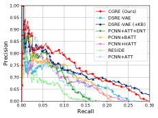
(a) NYT-520K

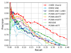
(b) NYT-570K

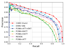
(c) GDS

Figure 4: PR curves for different models on NYT-520K, NYT-570K and GDS. Note that DSRE-VAE indicates the vanilla DSRE-VAE, and DSRE-VAE (+KB) indicates the the DSRE-VAE incorporating KB priors.

TABLE III: (%) P@N and AUC values of different models on NYT-520K, NYT-570K and GDS.

Model	NYT-520K				NYT-570K				GDS
	P@100	P@200	P@300	AUC	P@100	P@200	P@300	AUC	P@100	P@200	P@300	AUC
PCNN+ATT [8]	81.6	73.0	66.9	34.7	72.9	71.5	69.6	38.4	96.4	93.3	91.5	79.9
PCNN+HATT [26]	77.5	74.2	69.9	37.1	85.0	81.5	77.5	41.9	94.0	92.9	92.4	81.6
PCNN+BATT [10]	76.9	75.4	72.9	35.2	86.5	84.7	79.4	42.0	96.3	94.7	93.1	80.2
RESIDE [22]	69.3	67.5	63.4	35.5	81.4	74.9	73.8	41.5	98.4	96.4	95.2	86.8
DSRE-VAE [47]	74.0	74.5	71.6	38.6	80.0	76.0	75.6	44.6	96.9	96.7	96.3	87.6
DSRE-VAE (+KB) [47]	83.0	75.5	73.0	42.9	81.0	77.5	73.6	45.5	-	-	-	-
PCNN+ATT+ENT	79.4	74.7	68.3	35.5	83.7	81.4	77.5	47.0	93.9	93.7	93.5	84.9
CGRE (Ours)	82.7	80.3	76.5	41.7	88.9	86.4	81.8	51.9	98.6	98.1	97.7	90.5

3.4 Long Tail Evaluation

To fully demonstrate the effectiveness of CGRE on long-tail RE, we compare CGRE with several competitive baselines, including two vanilla DSRE models PCNN+ATT [8] and PCNN+ATT+ENT that ignore the long-tailed relations, and six state-of-the-art long-tailed RE models:

• PCNN+HATT [26]: the first model to apply relation hierarchies for long-tailed RE;

• PCNN+KATT [27]: a model that utilizes GCNs to encode relation hierarchies and applies knowledge graph embeddings for initialization;

• PA-TRP [28]: a model that learns relation prototypes from unlabeled texts for embedding relation hierarchies;

• CoRA [29]: a model that uses sentence embeddings to generate the representations for each node in relation hierarchies;

• ToHRE [54]: a model that applies a top-down classification strategy to explore relation hierarchies;

• DPEN [55]: a model that aggregates relations and entity types by stages to dynamically enhance the classifier.

Note that the first five models are all based on the relation hierarchy.

TABLE IV: (%) Accuracy of Hits@K on relations with training instances fewer than 100/200.

Training Instances	$<$100			$<$200
Hits@K (Macro)	10	15	20	10	15	20
PCNN+ATT [8]	$<$5.0	7.4	40.7	17.2	24.2	51.5
PCNN+ATT+ENT	22.2	33.3	61.1	36.4	45.5	68.2
PCNN+HATT [26]	29.6	51.9	61.1	41.4	60.6	68.2
PCNN+KATT [27]	35.3	62.4	65.1	43.2	61.3	69.2
PA-TRP [28]	63.9	70.3	72.2	66.7	72.3	73.8
CoRA [29]	59.7	63.9	73.6	65.4	69.0	77.4
ToHRE [54]	62.9	75.9	81.4	69.7	80.3	84.8
DPEN [55]	57.6	62.1	66.7	64.1	68.0	71.8
CGRE (Ours)	77.8	77.8	87.0	81.8	81.8	89.4

Following the previous studies [26, 27], we adopt Hit@K metric on NYT-570K to evaluate the performance on long-tailed relations. We extract the relations that have few than 100/200 training instances from the test set. Then Hits@K metric, which measures the probability that the true label falls in the top-$K$ recommendations of the model, is applied over these long-tailed relations. From the results in Table IV, we observe:

(1) effectiveness of modeling latent dependencies among relations. PCNN+ATT and PCNN+ATT+ENT give the worst results, showing the ineffectiveness of vanilla denoising models on long-tailed relations. By modeling the latent dependencies among relations, the performance improves significantly, but is still far from satisfactory.

(2) advantages of the constraint graph over the relation hierarchical tree. Based on the constraint graph, CGRE significantly and consistently outperforms all the previous relation hierarchy-based models. This confirms the advantages of the constraint graph for modeling dependencies among relations, which could be further amplified via the GCN.

(3) superiority of CGRE over DPEN in utilizing type information. As compared with DPEN, which also utilizes entity types to transfer information across relations, CGRE achieves significant and consistent performance superiority for long-tailed RE. We believe this performance gap stems mainly from the distinction in how the methods model and utilize type information. DPEN models the connections between entity types and relations implicitly, while CGRE makes these explicit via the constraint graph. Also, DPEN aggregates the features of entity types and relations by stages with a specific dynamic parameter generator, while CGRE adopts GCNs to achieve this objective directly.

As described in the aforementioned observations, long-tailed RE is still an intractable challenge even for the state-of-art DSRE models. A feasible solution is modeling intrinsic dependencies between the relations to transfer information from data-rich relations to data-poor relations, and the design of relation dependency structure is one of the key to modeling. With outstanding performance, the relation hierarchy seems to be the indispensable foundation of long-tailed RE frameworks [26, 27, 28, 29, 54], however, it is not the only option. In this work, we confirm the constraint graph is also a novel and effective structure for modeling latent dependencies between relations. Further, we believe there are still many promising relation dependency structures deserving extensive exploration.

TABLE V: (%) P@N on NYT-520K with different bag sizes.

Bag Size	One				Two				All
P@N	100	200	300	Mean	100	200	300	Mean	100	200	300	Mean
PCNN+ATT [8]	74.0	65.0	61.3	66.8	78.0	69.0	65.7	70.9	83.0	69.5	67.0	73.2
PCNN+HATT [26]	75.0	70.0	66.0	70.3	76.0	73.5	67.7	72.4	77.0	73.5	69.0	73.2
PCNN+BATT [10]	74.0	65.0	63.7	67.6	81.0	72.0	67.4	72.6	86.0	75.5	68.3	76.6
RESIDE [22]	68.0	67.5	63.3	66.3	65.0	61.5	58.0	61.5	70.0	65.5	58.0	64.5
DSRE-VAE [47]	79.0	70.0	63.3	70.6	77.0	70.0	66.0	71.0	79.0	75.5	69.0	74.5
DSRE-VAE (+KB) [47]	85.0	73.5	67.0	75.2	88.0	77.0	69.7	78.2	92.0	80.5	73.0	81.8
PCNN+ATT+ENT	78.0	68.0	66.0	70.7	79.0	70.0	64.0	71.0	79.0	70.5	66.7	72.1
CGRE (Ours)	86.0	74.5	68.0	76.2	88.0	76.0	71.7	78.6	88.0	77.5	73.3	79.6

TABLE VI: (%) P@N on NYT-570K with different bag sizes.

Bag Size	One				Two				All
P@N	100	200	300	Mean	100	200	300	Mean	100	200	300	Mean
PCNN+ATT [8]	73.3	69.2	60.8	67.8	77.2	71.6	66.1	71.6	76.2	73.1	67.4	72.2
PCNN+HATT [26]	84.0	76.0	69.7	76.6	85.0	76.0	72.7	77.9	88.0	79.5	75.3	80.9
PCNN+BATT [10]	86.8	77.6	73.9	79.4	91.2	79.2	75.4	81.9	91.8	84.0	78.7	84.8
RESIDE [22]	80.0	75.5	69.3	74.9	83.0	73.5	70.6	75.7	84.0	78.5	75.6	79.4
DSRE-VAE [47]	79.0	68.5	65.7	71.1	74.0	72.5	69.3	71.9	77.0	72.5	67.3	72.3
DSRE-VAE (+KB) [47]	79.0	72.0	65.7	72.2	81.0	74.0	66.7	73.9	88.0	74.0	70.7	77.6
PCNN+ATT+ENT	87.0	84.0	80.7	83.9	89.0	85.5	81.3	85.3	91.0	87.0	83.3	87.1
CGRE (Ours)	95.0	88.5	85.0	89.5	95.0	90.0	84.7	89.9	94.0	92.5	88.3	91.6

3.5 Quantitative Analysis of Selective Attention Mechanisms

In this section, we quantitatively evaluate the effects of selective attention mechanism on DSRE, to demonstrate the performance of our designed constraint-aware attention mechanism.

3.5.1 Performance of Selective Attention Mechanisms

We conduct top-N evaluations on the bags containing different number of sentences, to compare the performance of different selective attention mechanisms. Following the previous works [8, 22, 26, 10], we randomly select one / two / all sentences for each test entity pair with more than two sentences to construct three new test sets, on which we calculate P@N for these methods.

We report the results on NYT-520K and NYT-570K in Table IV and V. For the bags of size one, these selective attention mechanisms are ineffective, since they operate at the sentence level. As the bag size increases, selective attention mechanisms provide increasing performance improvements of bag-level DSRE. Across different bag sizes, CGRE achieves performance comparable with DSRE-VAE (+KB), and significantly outperforms other selective attention-based models. These results demonstrate the effectiveness of our constraint-aware attention mechanism.

3.5.2 Evaluation with Different Noise Ratios

We further quantitatively evaluate the performance of the proposed constraint-aware attention mechanism on bags with different noise ratios, using the analytical framework proposed by [56].

This analytical framework requires label-clean test data for quantitative evaluation. In this work, instead of creating a new dataset from scratch, we experiment with the existing NYT-H dataset because it provides human-annotated test data. NYT-H consists of a training set containing 96,831 instances (14,012 entity pairs) and a test set containing 9,955 instances (3,548 entity pairs), involving 21 relations (excluding NA).

In this experiment, we adopt two evaluation metrics as follows:

• Attention Accuracy (AAcc). The key goal of the selective attention mechanism is to dynamically assign higher weights to valid sentences and lower weights to noisy sentences, and AAcc is designed for measuring this ability. Given a bag $\mathcal{B}_{i}=\{s_{i1},\ldots,s_{in_{s}}\}$ containing both valid and noisy sentences and the attention weights $\{\alpha_{i1},\ldots,\alpha_{in_{s}}\}$ over the sentences, AAcc of this bag is formally defined as follows:

  $$\mathrm{AAcc}_{i}=\frac{\sum_{j=1}^{n_{s}}\sum_{k=1}^{n_{s}}\mathbf{I}\left(z_{ij}\right)\mathbf{I}\left(1-z_{ik}\right)\mathbf{I}\left(\alpha_{ij}>\alpha_{ik}\right)}{\sum_{j=1}^{n_{s}}\mathbf{I}\left(z_{ij}\right)\sum_{j=1}^{n_{s}}\mathbf{I}\left(1-z_{ij}\right)}$$

  where $\mathbf{I}(\cdot)$ is an indicator function and $z_{ij}$ is a flag indicating whether the sentence $s_{ij}$ is valid. The numerator counts how many valid-noisy sentence pairs show higher attention weight on the valid sentence, and the denominator is the number of valid-noisy sentence pairs is the bag $\mathcal{B}_{i}$. Then AAcc of the whole test set is computed as $\mathrm{AAcc}=\frac{\sum^{n}_{i=1}\mathrm{AAcc}_{i}}{n}$, where $n$ is total number of bags.

• F1-Score. We adopt the F1-Score instead of AUC (which is used in [56]) as the evaluation metric, since the test labels are human-annotated. Firstly, we calculate F1-Score on the whole test set as a baseline. Then we construct three test sets with zero / one / all valid sentences in each bag. Finally, we calculate F1-Scores on these three datasets. We emphasize that for the case of zero, a prediction equaling the bag relation is incorrect, since there are no sentences expressing the relation in the bag.

TABLE VII: (%) AAcc and F1-Scores results on NYT-H, where Orig. indicates the original test set, Zero indicates the test set in which no sentences are valid, One indicates the test set in which only one sentence is valid in each bag, All indicates the test set in which all sentences are valid.

Model	AAcc	F1-Score
		Orig.	Zero	One	All
PCNN+ATT[8]	52.9	60.5	63.9	72.4	75.7
PCNN+CATT	57.3	66	71.1	78.5	80.2

We present the results in Table VII, in which CGRE is renamed PCNN+CATT (constraint-aware attention), to highlight the attention mechanisms used. From Table VII, we observe that:

(1) PCNN+CATT achieves 4.2% AAcc improvements over PCNN+ATT, demonstrating that the stronger ability of CATT over ATT to recognize the noisy sentences and to dynamically reduce their attention weights.

(2) PCNN+CATT achieves 5.5%, 7.2%, 6.1% and 4.5% F1-Score improvements over PCNN+ATT, in the settings of Orig., Zero, One and All, respectively. Compared with the original selective attention mechanism[8], our designed constraint-aware attention mechanism shows stronger abilities to identify valid sentences in various noisy environments. Specially, all sentences in Zero are valid, so it is satisfactory that any sentence obtains higher attention weight. However, PCNN+CATT still achieve a significant advantage in Zero. The reason we speculate is that CATT tends to assign higher attention weights to the easily recognized valid sentences.

3.6 Ablation Study

We perform ablation studies to further evaluate the effects and contributions of different components of CGRE. Note that all ablation experiments are conducted on NYT-520K, for a more accurate evaluation.

3.6.1 Effect of Backbone Models

We evaluate the effects of different backbone models on the performance of CGRE. We experiment with three widely used sentence encoders CNN[57], PCNN[42] and BERT[58], and three representative graph encoders GCN[39], GAT[59] and SAGE[60]. Compared with GCN, GAT dynamically assigns different attention weights to different neighbors in aggregation computation, while SAGE generates embeddings by sampling and aggregating neighboring features instead of training individual embeddings for each node. Note that the entity-aware word embedding[41] is only applied in CNN and PCNN, since BERT has integrated word embeddings.

TABLE VIII: (%) AUC and macro accuracy of Hits@K of different backbone models on NYT-520K, where None indicate the case without the constraint graph (e.g., CNN+None is equivalent to CNN+ATT+ENT), playing the baseline role, and $<$100/$<$200 indicates the long-tailed relations with training instances fewer than 100/200.

Encoder		$<$100		$<$200		AUC
Sent.	Graph	Hits@5	Hits@10	Hits@5	Hits@10
CNN	None	7.5	20.0	19.2	32.4	35.0
	GCN	17.5	40.0	31.2	50.0	38.2
	GAT	27.5	40.0	39.6	50.0	38.7
	SAGE	24.2	40.0	34.0	50.0	37.3
PCNN	None	15.0	35.0	28.2	45.8	35.5
	GCN	19.2	40.0	32.6	50.0	41.7
	GAT	23.3	40.0	35.2	50.0	41.8
	SAGE	22.5	65.0	34.5	70.8	39.3
BERT	None	10.0	30.0	25.0	41.7	46.1
	GCN	31.7	36.7	43.1	47.2	46.8
	GAT	23.3	40.0	36.1	50.0	48.9
	SAGE	25.0	45.0	36.6	54.2	47.2

We report the experimental results in Table VIII, from which we observe that:

(1) compared with the baselines without the constraint graph, any combination achieves significant and consistent improvements on performance of denoising and long-tailed RE. This strongly suggests the effectiveness of the proposed constraint graph;

(2) among the sentence encoders, BERT shows huge advantages on overall performance against noise and top-5 hit rate on long-tailed relations. However, CNN and PCNN also show competitive performance on the top-10 hit rate;

(3) among the graph encoders, GAT achieves the highest anti-noise performance, independently of the sentence encoder choices. In terms of long-tailed RE, GAT provides the highest improvements for CNN and PCNN, while GCN and SAGE show more benefits for BERT;

(4) the BERT-based CGRE variants achieve significant improvements over the previous Transformer architectural model, DISTRE [45], which achieves an AUC value of 42.2% on NYT-520K.

Although BERT and GAT show significant superiority in this ablation experiment, we still utilize PCNN and GCN as the sentence and graph encoders of vanilla CGRE, for their high efficiency and acceptable accuracy. We retain the choices of other backbone models as the variants of CGRE.

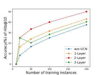
(a) Performance of GCNs with different layer numbers.

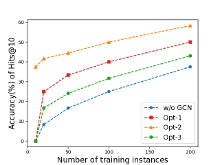
(b) Performance of GCNs with different output options.

Figure 5: Performance on the long-tailed relations with different number of training instances.

3.6.2 Effect of the Constraint Graph

As effectiveness of the constraint graph has been confirmed in Sec. 3.6.1, we further explore the effects of different information (i.e., type information and constraint information) in the constraint graph. We briefly denote the CGRE without the constraint graph as Base, which is equivalent to PCNN+ATT+ENT. To evaluate the effect of type information, we build Base+Type, which concatenates the sentence representations with the corresponding type representations, and then transforms the dimension of the concatenating representation to match that of the relation representation for attention computation. To evaluate the effect of constraint information, we build Base+Const, which is identical to Base, except that instances violating constraints are removed during training and predicted as NA with 100% probability during testing.

We present the results of AUC and macro accuracy of Hits@K in Table IX, from which we observe that:

(1) both the external information of entity types and relation constraints provide significant improvements on denoising and long-tailed RE;

(2) improvements on long-tailed RE from type information and constraint information are comparable. However, type information shows significant advantages (with 2.4% AUC improvement over constraint information) on overall performance against noise;

(3) compared with directly integrating the type information or the hard constraint strategy, our proposed CGRE organically combines these two kinds of information to achieve significant improvements in terms of denoising and long-tailed RE.

TABLE IX: (%) AUC and macro accuracy of Hits@K of different variants on NYT-520K.

Model	$<$100		$<$200		AUC
	Hits@5	Hits@10	Hits@5	Hits@10
Base	5.0	5.0	15.3	20.8	34.7
Base+Type	$<$5.0	27.8	16.2	40.9	39.4
Base+Const	12.5	25.0	26.2	37.5	37.0
CGRE	19.2	40.0	32.6	50.0	41.7

3.6.3 Effect of GCNs

To investigate the effect of the integration mechanism of GCNs on knowledge transfer between relations, we evaluate the long-tailed RE performance of GCNs with different layer numbers and different output options. We denote CGRE without GCN as w/o GCN, in which the input embeddings $\mathbf{V}^{(0)}$ are directly output, and denote CGRE with a $k$-layer GCN as k-Layer. For a $2$-layer GCN, we design 3 different output options:

• Opt-1 directly take the representations of last layer, i.e. $\mathbf{V}^{(2)}$, for output;

• Opt-2 concatenates the representations of last 2 layers, i.e. $[\mathbf{V}^{(1)};\mathbf{V}^{(2)}]$, for output;

• Opt-3 concatenates the representations of last 3 layers, i.e. $[\mathbf{V}^{(0)};\mathbf{V}^{(1)};\mathbf{V}^{(2)}]$, for output.

To ensure dimensional matching, the concatenated vectors are transformed by a linear layer before output.

From the results shown in Figure 5, we observe that:

(1) GCN-based variants consistently outperform CGRE w/o GCN. This confirms the intuition that the neighborhood integration mechanism of GCN could effectively propagate rich information from the head relations to the long-tailed relations.

(2) due to over-smoothing, the increase of number of GCN layers may hurt the performance. As shown in Fig. 5(a), the 2-layer GCN achieve the best performance in our experiments;

(3) Fig. 5(b) shows a huge advantage of Opt-2 on long-tailed RE. We speculate the reason is that concatenation with the low-layer integrated representations could enhance the information propagation and feature learning, while concatenation with the non-integrated embeddings may impedes the knowledge transfer among relations.

TABLE X: Examples for case study. The column Satisfactory indicates whether the sentence satisfies the constraint, and column the Correct indicates whether the label is correct. The words in bold represent the target entities. In Entity Type, NORP implies nationalities, religious or political groups, LANG implies languages, and GPE implies countries, cities or states.

ID	Sentence	Entity Type	Satisfactory	Correct	Score
$s_{1}$	With the city so influenced by chinese and japanese culture, asian cuisine is always an excellent bet.	(NORP, NORP)	Yes	Yes	0.967
$s_{2}$	In the last several years, the site has housed a french restaurant, an asian buffet, and as of about three months ago a japanese restaurant…	(NORP, NORP)	Yes	No	0.009
$s_{3}$	”Three extremes”, 125 minutes in japanese, korean, mandarin and cantonese, this trilogy provides a sampler of short horror films from high-profile asian directors.	(LANG, NORP)	No	No	0.003
Relation: /people/ethnicity/included_in_group		Constraint: (LANG, NORP)
$s_{4}$	Herzen was tireless in his crusade for freeing russia ’s serfs and refor- ming russian society.	(NORP, GPE)	Yes	Yes	0.695
$s_{5}$	The russian debate on the treaty is subtly shifting, with new attention to the missiles russia will really need.	(NORP, GPE)	Yes	No	0.032
$s_{6}$	In st.petersburg, russia, summer advantage is giving teenagers early college credit for russian language classes.	(LANG, GPE)	No	No	0.007
Relation: /people/ethnicity/geographic_distribution		Constraint: (NORP, GPE)

3.6.4 Effect of Entity-aware Word Embedding

The entity-aware word embedding proposed by [41] shows huge advantages on NYT-570K, and has been applied in several recent works[29, 54]. In this study, we comprehensively evaluate the performance of this module. As shown in Fig. 4 and Table III, its advantages on NYT-520K and GDS are not as huge as that on NYT-570K, which contains many overlapping entity pairs. This suggests that the overall improvements provided by entity-aware word embedding are mainly due to rote memorization of the entity pairs occurring in the training set. However, the positive effectiveness of the module should not be entirely denied, since it provides 0.8% and 5.0% AUC improvements on NYT-520K and GDS, respectively. Hence, we still retain this module in vanilla CGRE for its slight improvements and plug-and-play property.

We further investigate the effect of the smoothing coefficient $\lambda$, which balances the contribution of entity information and word information. We experiment with $\lambda\in[0,20]$, and present the AUC trend in Fig 6. It is clear that the selection of $\lambda$ has a significant impact on the overall performance. We observe that the two peaks occur at $\lambda=3$ and $17$, while the trough occurs at $\lambda=8$.

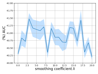
Figure 6: AUC for different smoothing coefficient $\lambda$.

3.7 Case Study

We present some examples to demonstrate how our constraint-aware attention combines the semantic and constraint information. As shown in Table X, the incorrect sentences with constraint violation ($s_{3}$ and $s_{6}$) or semantic inconsistency ($s_{2}$ and $s_{5}$) are assigned lower scores, while the correct sentences ($s_{1}$ and $s_{4}$) score higher. With the constraint-aware attention mechanism, CGRE can effectively recognize the valid instances from noisy data.

4 Related Work

To automatically obtain large scale labeled training data, [7] proposed distant supervision. However, the relation labels collected through distant supervision are not only noisy but also extremely unbalanced. Therefore, denoising and long-tailed RE become two major challenges in DSRE.

4.1 Denoising in DSRE.

Multi-instance learning (MIL), aiming to extract relations of an entity pair from a sentence bag instead of a single sentence, is a popular approach to alleviate the noisy labeling problem [25, 61, 62]. Under the MIL framework, various denoising methods are proposed, including selective attention mechanism [8, 10], external information integration [19, 22] and robust context encoders [42, 45]. Different from the bag-level prediction of MIL, some studies [11, 63] attempt to predict relations at sentence level by selecting trustable instances from training data.

In this work, we mainly focus on the bag-level prediction. There are two main differences between CGRE and the above MIL methods: (1) rather than treat each relation label separately, CGRE attempts to mine the latent dependencies between relations; (2) the attention mechanism of CGRE integrates the prior constraint information, which is effective for improving the noise immunity of RE models.

4.2 Long-tailed relation extraction in DSRE.

[64] develops an RE system, which can automatically learn the rules for long-tailed relations from Web. To generate fewer but more precise rules, [65] applies explanation-based learning to improve the RE system. However, the above methods merely handle each relation in isolation, regardless of the implicit associations between relations. Therefore, some recent works [26, 27, 29, 54] attempt to mine the semantic dependencies between relations from the relation hierarchical tree. To achieve the same objective without the relation hierarchical tree, [55] proposed DPEN, utilizing entity types to implicitly transfer information across different relations. Although these works achieve significant improvement for long-tailed relations, they are still far from satisfactory.

Different from relation hierarchies that mainly contain the hierarchical information between labels, the proposed constraint graph involves not only the implicit connection information between labels, but also the explicit prior information of constraints. By integrating both kinds of information, our CGRE can effectively handle the noisy and long-tailed labels.

4.3 Type constraint information in DSRE.

Type information of entities showed great potential on relation extraction [36, 37]. Some works  [21, 22] explored the utilization of fine-grained entity type information to improve the robustness of DSRE models. However, these methods merely focus on the semantic information of types, i.e., they simply use type information as concatenating features to enrich the sentence semantic representation, but neglect the explicit constraint information, which can be effective for recognizing the noisy instances. On the contrary, [35] applies probabilistic soft logic to encode the type constraint information for denoising, but ignores the semantic information of entity types.

As compared with the above methods, CGRE can take full advantage of type information. With the constraint-aware attention mechanism, CGRE can combine the semantic and constraint information of entity types. Moreover, in CGRE, the entity types are used as bridges between the relations, enabling message passing between relation labels.

5 Conclusion and Futute Work

In this paper, we aim to address both the challenges of label noise and long-tailed relations in DSRE. We introduce a novel relation dependency structure, constraint graph, to model the dependencies between relations, and then propose a novel relation extraction framework, CGRE, to integrate the information from the constraint graph. Experimental results on two popular benchmark datasets have shown that:

(1) the constraint graph can effectively express the latent semantic dependencies between relation labels;

(2) our framework can take full advantage of the information in the constraint graph, significantly and consistently outperforming the competitive baselines in terms of denoising and long-tailed RE.

We believe our exploration for constraint graph shall shed light on future research directions, especially for long-tailed relation extraction.

Specifically, we plan to explore:

(1) structural extensions of the constraint graph. For example, it would be promising to further improve the performance of long-tailed RE by combining the constraint graph and the relation hierarchical tree;

(2) effective approaches to strengthen the constraint graph. As demonstrated in [27] and [47], KB priors are effective external information for improving DSRE. It is therefore desirable to integrate KB priors into the constraint graph for further performance improvements.

References

- [1] Y. Shen, N. Ding, H. Zheng, Y. Li, and M. Yang, “Modeling relation paths for knowledge graph completion,” IEEE Transactions on Knowledge and Data Engineering, 2020.
- [2] H. Xiao, Y. Chen, and X. Shi, “Knowledge graph embedding based on multi-view clustering framework,” IEEE Transactions on Knowledge and Data Engineering, vol. 33, no. 2, pp. 585–596, 2021.
- [3] Z. Jiang, Z. Dou, and J. Wen, “Generating query facets using knowledge bases,” IEEE Transactions on Knowledge and Data Engineering, vol. 29, no. 2, pp. 315–329, 2016.
- [4] D. V. Kalashnikov, Z. Chen, S. Mehrotra, and R. Nuray-Turan, “Web people search via connection analysis,” IEEE Transactions on Knowledge and Data Engineering, vol. 20, no. 11, pp. 1550–1565, 2008.
- [5] S. Hu, L. Zou, J. X. Yu, H. Wang, and D. Zhao, “Answering natural language questions by subgraph matching over knowledge graphs,” IEEE Transactions on Knowledge and Data Engineering, vol. 30, no. 5, pp. 824–837, 2018.
- [6] Y. Hua, Y. Li, G. Haffari, G. Qi, and T. Wu, “Few-shot complex knowledge base question answering via meta reinforcement learning,” in Proceedings of EMNLP, 2020, pp. 5827–5837.
- [7] M. Mintz, S. Bills, R. Snow, and D. Jurafsky, “Distant supervision for relation extraction without labeled data,” in Proceedings of ACL-IJCNLP, 2009, pp. 1003–1011.
- [8] Y. Lin, S. Shen, Z. Liu, H. Luan, and M. Sun, “Neural relation extraction with selective attention over instances,” in Proceedings of ACL, 2016, pp. 2124–2133.
- [9] C. Yuan, H. Huang, C. Feng, X. Liu, and X. Wei, “Distant supervision for relation extraction with linear attenuation simulation and non-iid relevance embedding,” in Proceedings of AAAI, 2019, pp. 7418–7425.
- [10] Z. Ye and Z. Ling, “Distant supervision relation extraction with intra-bag and inter-bag attentions,” in Proceedings of NAACL-HLT, 2019, pp. 2810–2819.
- [11] J. Feng, M. Huang, L. Zhao, Y. Yang, and X. Zhu, “Reinforcement learning for relation classification from noisy data,” in Proceedings of AAAI, 2018, pp. 5779–5786.
- [12] Z. Li, Y. Sun, S. Tang, C. Zhang, and H. Ma, “Adaptive graph convolutional networks with attention mechanism for relation extraction,” in Proceedings of IJCNN. IEEE, 2020, pp. 1–8.
- [13] Y. Wu, D. Bamman, and S. Russell, “Adversarial training for relation extraction,” in Proceedings of EMNLP, 2017, pp. 1778–1783.
- [14] P. Qin, W. Xu, and W. Y. Wang, “Dsgan: generative adversarial training for distant supervision relation extraction,” in Proceedings of ACL, 2018, pp. 496–505.
- [15] P. Li, X. Zhang, W. Jia, and H. Zhao, “Gan driven semi-distant supervision for relation extraction,” in Proceedings of NAACL, 2019, pp. 3026–3035.
- [16] D. Puspitaningrum, “Improving performance of relation extraction algorithm via leveled adversarial pcnn and database expansion,” in Proceedings of CITSM, vol. 7. IEEE, 2019, pp. 1–6.
- [17] Q. Zhang and H. Wang, “Noise-clustered distant supervision for relation extraction: A nonparametric bayesian perspective,” in Proceedings of EMNLP, 2017, pp. 1808–1813.
- [18] Y. Shang, H. Y. Huang, X. Mao, X. Sun, and W. Wei, “Are noisy sentences useless for distant supervised relation extraction?” in Proceedings of AAAI, 2020, pp. 8799–8806.
- [19] G. Ji, K. Liu, S. He, J. Zhao et al., “Distant supervision for relation extraction with sentence-level attention and entity descriptions,” in Proceedings of AAAI, vol. 3060, 2017.
- [20] L. Hu, L. Zhang, C. Shi, L. Nie, W. Guan, and C. Yang, “Improving distantly-supervised relation extraction with joint label embedding,” in Proceedings of EMNLP-IJCNLP, 2019, pp. 3812–3820.
- [21] Y. Liu, K. Liu, L. Xu, and J. Zhao, “Exploring fine-grained entity type constraints for distantly supervised relation extraction,” in Proceedings of COLING, 2014, pp. 2107–2116.
- [22] S. Vashishth, R. Joshi, S. S. Prayaga, C. Bhattacharyya, and P. Talukdar, “Reside: improving distantly-supervised neural relation extraction using side information,” in Proceedings of EMNLP, 2018, pp. 1257–1266.
- [23] J. Kuang, Y. Cao, J. Zheng, X. He, M. Gao, and A. Zhou, “Improving neural relation extraction with implicit mutual relations,” in Proceedings of ICDE. IEEE Computer Society, 2020, pp. 1021–1032.
- [24] G. Wang, W. Zhang, R. Wang, Y. Zhou, X. Chen, W. Zhang, H. Zhu, and H. Chen, “Label-free distant supervision for relation extraction via knowledge graph embedding,” in Proceedings of EMNLP, 2018, pp. 2246–2255.
- [25] S. Riedel, L. Yao, and A. McCallum, “Modeling relations and their mentions without labeled text,” in Proceedings of ECML-PKDD, 2010, pp. 148–163.
- [26] X. Han, P. Yu, Z. Liu, M. Sun, and P. Li, “Hierarchical relation extraction with coarse-to-fine grained attention,” in Proceedings of EMNLP, 2018, pp. 2236–2245.
- [27] N. Zhang, S. Deng, Z. Sun, G. Wang, X. Chen, W. Zhang, and H. Chen, “Long-tail relation extraction via knowledge graph embeddings and graph convolution networks,” in Proceedings of NAACL-HLT, 2019, pp. 3016–3025.
- [28] Y. Cao, J. Kuang, M. Gao, A. Zhou, Y. Wen, and T.-S. Chua, “Learning relation prototype from unlabeled texts for long-tail relation extraction,” IEEE Transactions on Knowledge and Data Engineering, 2021.
- [29] Y. Li, T. Shen, G. Long, J. Jiang, T. Zhou, and C. Zhang, “Improving long-tail relation extraction with collaborating relation-augmented attention,” in Proceedings of COLING, 2020, pp. 1653–1664.
- [30] I. Hendrickx, S. N. Kim, Z. Kozareva, P. Nakov, D. Ó. Séaghdha, S. Padó, M. Pennacchiotti, L. Romano, and S. Szpakowicz, “Semeval-2010 task 8: Multi-way classification of semantic relations between pairs of nominals,” in Proceedings of the Workshop on Semantic Evaluations: Recent Achievements and Future Directions (SEW-2009), 2009, pp. 94–99.
- [31] Y. Zhang, V. Zhong, D. Chen, G. Angeli, and C. D. Manning, “Position-aware attention and supervised data improve slot filling,” in Proceedings of EMNLP, 2017, pp. 35–45.
- [32] X. Han, H. Zhu, P. Yu, Z. Wang, Y. Yao, Z. Liu, and M. Sun, “Fewrel: A large-scale supervised few-shot relation classification dataset with state-of-the-art evaluation,” in Proceedings of EMNLP, 2018, pp. 4803–4809.
- [33] T. Gao, X. Han, H. Zhu, Z. Liu, P. Li, M. Sun, and J. Zhou, “Fewrel 2.0: Towards more challenging few-shot relation classification,” in Proceedings of EMNLP-IJCNLP, 2019, pp. 6251–6256.
- [34] J. Bang Jensen and G. Z. Gutin, Digraphs: theory, algorithms and applications. Springer Science & Business Media, 2008.
- [35] K. Lei, D. Chen, Y. Li, N. Du, M. Yang, W. Fan, and Y. Shen, “Cooperative denoising for distantly supervised relation extraction,” in Proceedings of COLING, 2018, pp. 426–436.
- [36] H. Peng, T. Gao, X. Han, Y. Lin, P. Li, Z. Liu, M. Sun, and J. Zhou, “Learning from context or names? an empirical study on neural relation extraction,” in Proceedings of EMNLP, 2020, pp. 3661–3672.
- [37] Z. Zhong and D. Chen, “A frustratingly easy approach for entity and relation extraction,” in Proceedings of NAACL-HLT, 2021, pp. 50–61.
- [38] J. Qu, W. Hua, D. Ouyang, and X. Zhou, “A noise-aware method with type constraint pattern for neural relation extraction,” IEEE Transactions on Knowledge and Data Engineering, 2021.
- [39] T. N. Kipf and M. Welling, “Semi-supervised classification with graph convolutional networks,” in Proceedings of ICLR, 2017.
- [40] S. Pradhan, A. Moschitti, N. Xue, H. T. Ng, A. Björkelund, O. Uryupina, Y. Zhang, and Z. Zhong, “Towards robust linguistic analysis using ontonotes,” in Proceedings of CoNLL, 2013, pp. 143–152.
- [41] Y. Li, G. Long, T. Shen, T. Zhou, L. Yao, H. Huo, and J. Jiang, “Self-attention enhanced selective gate with entity-aware embedding for distantly supervised relation extraction,” in Proceedings of AAAI, 2020, pp. 8269–8276.
- [42] D. Zeng, K. Liu, Y. Chen, and J. Zhao, “Distant supervision for relation extraction via piecewise convolutional neural networks,” in Proceedings of EMNLP, 2015, pp. 1753–1762.
- [43] D. Marcheggiani and I. Titov, “Encoding sentences with graph convolutional networks for semantic role labeling,” in Proceedings of EMNLP, 2017, pp. 1506–1515.
- [44] A. Akbik, T. Bergmann, D. Blythe, K. Rasul, S. Schweter, and R. Vollgraf, “Flair: an easy-to-use framework for state-of-the-art nlp,” in Proceedings of NAACL, 2019, pp. 54–59.
- [45] C. Alt, M. Hübner, and L. Hennig, “Fine-tuning pre-trained transformer language models to distantly supervised relation extraction,” in Proceedings of ACL, 2019, pp. 1388–1398.
- [46] F. Bai and A. Ritter, “Structured minimally supervised learning for neural relation extraction,” in Proceedings of NAACL, 2019, pp. 3057–3069.
- [47] F. Christopoulou, M. Miwa, and S. Ananiadou, “Distantly supervised relation extraction with sentence reconstruction and knowledge base priors,” in Proceedings of NAACL, 2021, pp. 11–26.
- [48] X. Zhang, T. Liu, P. Li, W. Jia, and H. Zhao, “Robust neural relation extraction via multi-granularity noises reduction,” IEEE Transactions on Knowledge and Data Engineering, vol. 33, no. 9, pp. 3297–3310, 2021.
- [49] S. Jat, S. Khandelwal, and P. Talukdar, “Improving distantly supervised relation extraction using word and entity based attention,” arXiv preprint arXiv:1804.06987, 2018.
- [50] K. Hao, B. Yu, and W. Hu, “Knowing false negatives: An adversarial training method for distantly supervised relation extraction,” in Proceedings of EMNLP, 2021, pp. 9661–9672.
- [51] X. Glorot and Y. Bengio, “Understanding the difficulty of training deep feedforward neural networks,” in Proceedings of AISTATS, 2010, pp. 249–256.
- [52] N. Srivastava, G. Hinton, A. Krizhevsky, I. Sutskever, and R. Salakhutdinov, “Dropout: a simple way to prevent neural networks from overfitting,” JMLR, vol. 15, no. 1, pp. 1929–1958, 2014.
- [53] X. Ling and D. S. Weld, “Fine-grained entity recognition,” in Proceedings of AAAI, 2012, pp. 94–100.
- [54] E. Yu, W. Han, Y. Tian, and Y. Chang, “Tohre: A top-down classification strategy with hierarchical bag representation for distantly supervised relation extraction,” in Proceedings of COLING, 2020, pp. 1665–1676.
- [55] Y. Gou, Y. Lei, L. Liu, P. Zhang, and X. Peng, “A dynamic parameter enhanced network for distant supervised relation extraction,” Knowledge-Based Systems, vol. 197, p. 105912, 2020.
- [56] Z. Hu, Y. Cao, L. Huang, and T.-S. Chua, “How knowledge graph and attention help? a qualitative analysis into bag-level relation extraction,” in Proceedings of ACL-IJCNLP, 2021, pp. 4662–4671.
- [57] D. Zeng, K. Liu, S. Lai, G. Zhou, and J. Zhao, “Relation classification via convolutional deep neural network,” in Proceedings of COLING, 2014, pp. 2335–2344.
- [58] J. D. M.-W. C. Kenton and L. K. Toutanova, “Bert: Pre-training of deep bidirectional transformers for language understanding,” in Proceedings of NAACL-HLT, 2019, pp. 4171–4186.
- [59] P. Veličković, G. Cucurull, A. Casanova, A. Romero, P. Liò, and Y. Bengio, “Graph attention networks,” in Proceedings of ICLR, 2018.
- [60] W. L. Hamilton, R. Ying, and J. Leskovec, “Inductive representation learning on large graphs,” in Proceedings of NeurIPS, 2017, pp. 1025–1035.
- [61] R. Hoffmann, C. Zhang, X. Ling, L. Zettlemoyer, and D. S. Weld, “Knowledge-based weak supervision for information extraction of overlapping relations,” in Proceedings of ACL, 2011, pp. 541–550.
- [62] M. Surdeanu, J. Tibshirani, R. Nallapati, and C. D. Manning, “Multi-instance multi-label learning for relation extraction,” in Proceedings of EMNLP-CoNLL, 2012, pp. 455–465.
- [63] W. Jia, D. Dai, X. Xiao, and H. Wu, “Arnor: attention regularization based noise reduction for distant supervision relation classification,” in Proceedings of ACL, 2019, pp. 1399–1408.
- [64] S. Krause, H. Li, H. Uszkoreit, and F. Xu, “Large-scale learning of relation-extraction rules with distant supervision from the web,” in ISWC, 2012, pp. 263–278.
- [65] Y. Gui, Q. Liu, M. Zhu, and Z. Gao, “Exploring long tail data in distantly supervised relation extraction,” in Natural Language Understanding and Intelligent Applications. Springer, 2016, pp. 514–522.