A novel nonlocal partial differential equation model of endothelial progenitor cell cluster formation during the early stages of vasculogenesis

Abstract

The formation of new vascular networks is essential for tissue development and regeneration, in addition to playing a key role in pathological settings such as ischemia and tumour development. Experimental findings in the past two decades have led to the identification of a new mechanism of neovascularisation, known as cluster-based vasculogenesis, during which endothelial progenitor cells (EPCs) mobilised from the bone marrow are capable of bridging distant vascular beds in a variety of hypoxic settings in vivo. This process is characterised by the formation of EPC clusters during its early stages and, while much progress has been made in identifying various mechanisms underlying cluster formation, we are still far from a comprehensive description of such spatio-temporal dynamics. In order to achieve this, we propose a novel mathematical model of the early stages of cluster-based vasculogenesis, comprising of a system of nonlocal partial differential equations including key mechanisms such as endogenous chemotaxis, matrix degradation, cell proliferation and cell-to-cell adhesion. We conduct a linear stability analysis on the system and solve the equations numerically. We then conduct a parametric analysis of the numerical solutions of the one-dimensional problem to investigate the role of underlying dynamics on the speed of cluster formation and the size of clusters, measured via appropriate metrics for the cluster width and compactness. We verify the key results of the parametric analysis with simulations of the two-dimensional problem. Our results, which qualitatively compare with data from in vitro experiments, elucidate the complementary role played by endogenous chemotaxis and matrix degradation in the formation of clusters, suggesting chemotaxis is responsible for the cluster topology while matrix degradation is responsible for the speed of cluster formation. Our results also indicate that the nonlocal cell-to-cell adhesion term in our model, even though it initially causes cells to aggregate, is not sufficient to ensure clusters are stable over long time periods. Consequently, new modelling strategies for cell-to-cell adhesion are required to stabilise in silico clusters. We end the paper with a thorough discussion of promising, fruitful future modelling and experimental research perspectives.

1 Introduction

The formation of new vascular networks is essential for tissue development and regeneration, as a functional vasculature is critical for tissue homeostasis. It is responsible for the delivery of oxygen and nutrients as well as the disposal of waste products. In addition, neovascularisation of local tissue is critical in a variety of pathological processes, among which are retinopathy, tumour growth, wound healing and soft-tissue ischemia. The development of a vascular network in localised solid tumours is particularly well known to promote further tumour growth and metastases. Therefore a better understanding of the mechanisms governing neovascularisation can help improve current therapeutic strategies, as well as identify new ones.

The two fundamental processes of neovascularisation are known as vasculogenesis, the de novo formation of a new vascular network, and angiogenesis, the formation of new blood vessels from pre-existing ones. While the distinction between these two processes has been clear since the early days of the field of study of vascular development [91], for a long time the term vasculogenesis was only associated with endothelial progenitor cells (EPCs)-mediated embryonic vasculogenesis, while blood vessels formation in adult organisms was believed to be formed predominantly, if not exclusively, via angiogenesis [88]. In the past 20 years great progress was made in understanding neovascularisation processes, in particular with the discovery of bone marrow-derived EPCs and postnatal vasculogenesis [9, 11, 10, 56, 83, 88, 101], for which a specific mechanism, here referred to as cluster-based vasculogenesis, has recently been proposed [16]. This newly identified mechanism of neovascularisation has been observed only in hypoxic settings in vivo, from development [84] to soft-tissue ischemia [109] to tumour vascularisation [115], and has been studied in detail by Blatchley et al. [16] in hypoxic gradients in vitro.

1.1 Cluster-based vasculogenesis

During this process, EPCs residing in the bone marrow are recruited in the circulation to the hypoxic site [10, 101], where they first organise into clusters. They then proceed to sprout from these clusters and, in combination with angiogenesis, form the new vascular network merging with pre-existing vasculature. The term “cluster-based” vasculogenesis was therefore proposed by Blatchley and coworkers [16] to highlight the key step of the process which well distinguishes it from classical “single-cell” vasculogenesis, during which sparse mature endothelial cells (ECs) directly reorganise into a vascular network [98].

While EPCs recruitment to angiogenic sites has been well studied, we are still far from understanding how clusters form and what drives sprouting from these clusters. Akita et al. [1] reported that EPC differentiation, secretion of angiogenic factors – such as Vascular Endothelial Growth Factor (VEGF) – and migration were enhanced by hypoxic conditioning, resulting in increased EPC cluster formation in hypoxia in vitro. Nevertheless, it was not until recently that Blatchley and coworkers proposed, together with the name here used, a two-step mechanism of cluster formation and stabilisation in hypoxic environments [16], illustrated in Figure 2. The proposed mechanism relies on the observation that in highly hypoxic environments the production of matrix metalloproteases (MMPs) is upregulated by the presence of reactive oxygen species (Figure 2B). This results in significant extracellular matrix (ECM) degradation responsible for EPCs aggregation into clusters, which are then stabilised by cell-to-cell adhesion (Figure 2C). EPC clusters were observed between 24 and 48 hours from the beginning of the experiments, presenting diameters in the range $100-400\,\mu$m– see Figure 1. Finally, after 48 hours, cell-to-matrix interactions lead to sprouting and network formation, particularly fostered by highly viscoelastic – where not degraded – ECM (Figure 2D). The final network, observed after 72 hours, was reported to be up to $500\,\mu$m in length, larger than previously observed ones formed via angiogenesis or single-cell vasculogenesis.

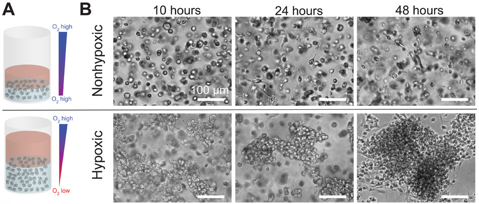
Figure 1: (A) Illustration summarising the 3D in vitro experimental set ups considered by Blatchley et al. [16] to study EPC cluster formation in hypoxic gradients (bottom) and in control nonhypoxic environments (top). (B) Corresponding experimental images displaying cluster formation after 48hours in hypoxic environments (bottom), while no clusters formed in nonhypoxic conditions (top). Illustrations and images are taken from Figure 1 in [16] under Creative Commons licence https://creativecommons.org/licenses/by-nc/4.0/.

Overall, cluster-based vasculogenesis has been shown to be of great importance in highly hypoxic tissues, as EPC clusters form in these regions far from pre-existing blood vessels and, after sprouting, function as a bridge for distant vascular beds, allowing for neovascularisation in physiological and pathological settings in which angiogenesis alone would not have sufficed.

While this is a great step forward in the understanding of cluster-based vasculogenesis, further work is required to reach an exhaustive comprehension of the process, as well as to unlock its full potential in therapeutic interventions in a variety of pathological process. On this regard, mathematical modelling can help elucidate the mechanisms behind network formation, serving as a proof of concept mean for newly developed theories [99], as well as steer experimental investigations towards the most promising research perspectives.

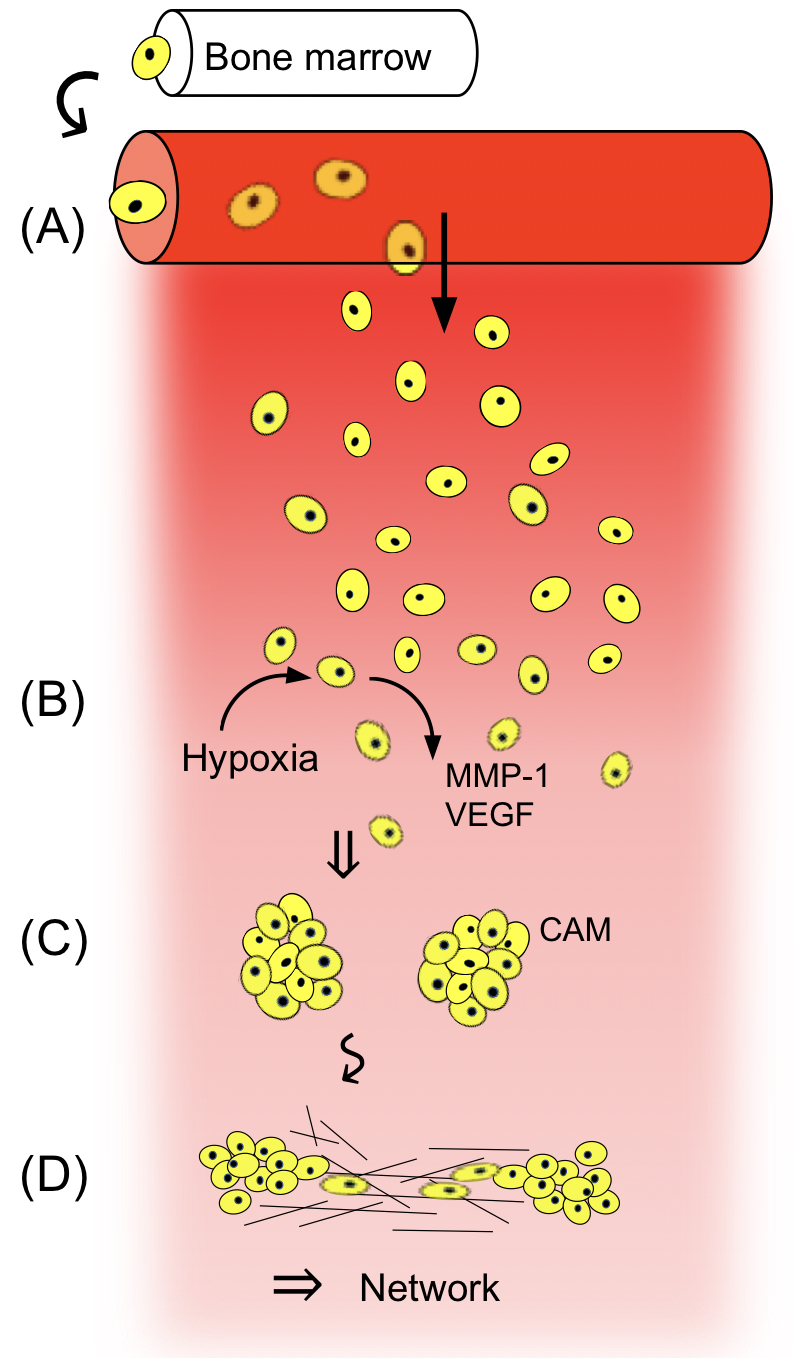
Figure 2: Summary of the steps of cluster-based vasculogenesis: (A) EPCs in the bone-marrow enter the circulation and reach the hypoxic site; (B) local hypoxia fosters EPC production of matrix degrading enzymes (MMP-1) and chemotactic agents (VEGF); (C) clusters form and are stabilised by cell-adhesion molecules (CAM); (D) cell-matrix interactions increase, sprouting from clusters occurs and a vascular network forms.

1.2 Mathematical modelling of vasculogenesis

While the mathematical model presented here is the first one formulated to study cluster-based vasculogenesis, many have been proposed to investigate in vitro single-cell vasculogenesis. Most models in the literature refer back to the work of Serini et al. [98] who investigate single-cell vasculogenesis in matrigel. During the early stages of this process, ECs were observed to undergo rapid motion, during which they maintained a round shape, until collision with their closest neighbours (3-6 hours). They then proceeded to reorganise into a continuous multicellular network, which can be represented as a collection of nodes connected by capillary chords (of characteristic length $\ell\approx 200\mu$m), exhibiting a more elongated morphology, until network stabilisation (9-15 hours). Note that cell proliferation and death of mature ECs can be neglected on such a short timescale in vitro. We first review key single-cell vasculogenesis models in the literature, referring the interested reader to more detailed reviews [3, 17, 31, 95], and then discuss model requirements to study cluster-based vasculogenesis.

Partial differential equation models of single-cell vasculogenesis

Continuum deterministic models in the extant literature can be categorised as Persistence and Endogenous Chemotaxis (PEC) models [4, 29, 38, 58, 62, 98], modelling the early stages of single-cell vasculogenesis, and mechanochemical models [64, 73, 74, 76], better suited to describe the late stages of the process, with the exception of the work by Tosin et al. [111] who proposed a comprehensive model.

First introduced by Serini and coworkers [38, 98], PEC models consist of a conservation equation for the EC density, a momentum equation describing changes in the EC velocity and a reaction-diffusion equation describing VEGF dynamics. In particular ECs are assumed to undergo persistent motion i.e. movement characterised by inertia in the velocity field, and this movement is modulated by friction between cells and substrate, density-dependent pressure and chemotaxis (with the VEGF being secreted by the cells themselves). Such models have so far helped to extrapolate information underlying the origin and structure of newly formed vascular networks, for instance relating the characteristic chord length $\ell$ to the VEGF diffusion coefficient $D_{c}$ and decay rate $\lambda_{c}$ with the formula $\ell=\sqrt{D_{c}(\lambda_{c})^{-1}}$ [4, 3, 38, 98], or investigating the minimum – and maximum – initial cell density required for network assembly [3, 29, 38, 58, 98]. In particular, as the initial cell density increases we observe a transition from a phase in which several disconnected structures appear to one in which a single connected structure appears. Detailed analyses of this phenomenon, known as percolative transition, revealed the critical EC density for transition to be around $100$ cells/mm² [29, 38]. Further increasing the initial cell density, instead of a well-defined network with thin chords, one may observe a cell monolayer with void areas called lacunae, a phenomenon referred to as “Swiss-cheese” transition [3, 98]. Linear stability analysis revealed chemotaxis to be the key destabilising force for lacunae fomation and pressure to be the main stabilising one [58]. Thanks to the pressure term, the Swiss-cheese transition can be predicted by PEC models about the critical initial cell density of $300$ cells/mm² [3].

On the other hand, mechanochemical models of vasculogenesis placed special emphasis on the role played by cell traction forces, thus being particularly suited for the later stages of vasculogenesis during which the mechanical interaction between the ECs and the ECM cannot be neglected. Mechanical models or vasculogenesis, following the work of Murray and coworkers [75], consist of a conservation equation for the EC density and one for the ECM density, a force-balance equation to describe changes in the cell-matrix displacement as cells pull on the ECM and, in the case of mechanochemical models, an additional reaction-diffusion equation describing VEGF dynamics [3]. Both ECs and ECM are assumed to be advected according to changes in the cell-matrix displacement, and ECs are also assumed to undergo strain-dependent movement [64, 74, 76], haptotaxis [76] and chemotaxis [64]. The ECM is modelled as a linear elastic or viscoelastic material, the substratum is introduced via external viscous drag or elastic forces, and cell traction either saturates or goes negative for large densities, the latter understood as modelling density-dependent pressure [76]. Linear stability analysis predicts instability of the homogeneous steady state, and in general lacunae formation, if the cell traction coefficient is high enough or the ECM Young modulus is low enough, and if the initial cell density is below a threshold value [3]. Haptotaxis was also indicated to have a destabilising effect [76], while the restoring forces and long range effects have a stabilising effect [3]. Note that while these models may predict cluster formation in the case of very high cell traction or very low ECM stiffness, such modelling frameworks are not compatible with the application here considered as they do not include any of the key mechanisms of early-stages cluster-based vasculogenesis.

Finally, Tosin et al. [111] proposed a PEC model with an external drag force in the momentum equation, slowing cells down as they move on the ECM, itself modelled as a linear elastic material. The model indicated cell adhesiveness to the substratuum to have a key role in network formation, with too high adhesiveness resulting in no network and too low adhesiveness affecting the stability of chords so that cells would eventually clusterise due to chemotaxis.

Cellular Potts models of single-cell vasculogenesis

Despite their lower analytical tractability, cellular Potts (CP) models have been widely used to study single-cell vasculogenesis over the years [17, 95]. These are lattice-based models, with simulations obtained via a Monte-Carlo method following energy minimisation principles, which track cell and ECM dynamics at the mesoscale. They are therefore particularly suited to investigate mechanisms occurring at the cell level, such as cell shape and cell-to-cell adhesion, which are difficult to describe with continuum models of macroscale dynamics and which may be crucial for single-cell vasculogenesis as the process involves a low number of cells [67]. These models predicted that elongated, adhesive cells can self-organised into vascular structures [81] and that these structures are faster achieved and stabilised thanks to endogenous chemotaxis [67]. Furthermore, these models confirm a correlation between the characteristic chord length and the VEGF diffusion rate, as previously indicated by PEC models. In the absence of cell elongation, the network formation is compromised and cells form islands. This observation is independent of whether elongation is imposed as a constraint [67] or it is a consequence of strong cell-to-cell adhesion [69], of preferential attraction of cells to elongated structures [106, 108, 107], or of cell traction, ECM stiffening and durotaxis [86, 116]. In the latter case, network formation was predicted for high enough cell traction compared to the ECM Young modulus, just like in mechanochemical models. Alternatively to cell elongation, cell polarisation resulting from cell adhesion-mediated saturation of chemotaxis may prevent clusters from forming [68, 70, 103]. Overall the work of Merks and coworkers pointed towards cell elongation, or polarisation and endogenous chemotaxis being essential for network formation.

Modelling the early stages cluster-based vasculogenesis

While much work has been conducted in order to better understand the mechanisms at the basis of single-cell vasculogenesis, and many of which are relevant to cluster-based vasculogenesis, recent experimental observations [16] seem to suggest that also other processes need to be considered when studying EPC cluster formation during the early stages of cluster-based vasculogenesis. While CP models may be preferred when studying a system comprising of few cells, EPCs actively proliferate and we therefore choose to study this process through the lenses of a continuum deterministic model, which is also more ameanable to analytical investigation. The model should include endogenous chemotaxis, MMP-mediated ECM degradation, cell-to-cell adhesion, EPC diffusion, proliferation and death, together with annexed ECM, VEGF and MMP dynamics. Note that while cell proliferation and ECM degradation have been included in previous models of vascular network formation [17, 33, 50, 64, 112], these have been formulated to study angiogenesis rather than vasculogenesis, which for instance require different initial conditions and exogenous rather than endogenous chemotaxis.

PEC models included chemotaxis in the momentum equation, but this implies that cells accelerate in chemical gradients, an assumption that might be unrealistic given the highly viscous, non-inertial environment of the ECM [67, 70]. We thus choose to follow standard modelling of chemotaxis in the flux term of the EPC density mass-balance equation, as done in mechanochemical models [3, 64], following the classic Patlak-Keller-Segel (PKS) model of diffusion and chemotaxis [53, 77]. As the PKS model is well-known for having solutions that blow up in finite time, a number of variations have been proposed in the literature [20, 57, 77], and we will hereby consider a modified version of the forms proposed by Hillen and Painter [47, 80] whereby chemotaxis is saturated in a tightly packed environment. While this results in a local description of chemotaxis, various nonlocal ones have also been proposed over the years, reviewed for instance in [26, 48, 79].

While CP models allowed for a mesoscopic description of cell-to-cell adhesion, during the development of PEC and mechanochemical models this biological process had not yet been explicitly modelled at the macroscopic scale. In 2006 Armstrong and coworkers published a seminal paper [7] proposing a continuum nonlocal description of intrapopulation and interpopulation cell adhesion. This was later adapted by Gerisch and Chaplain [42] to account for cell-to-cell and cell-to-matrix adhesion. The model relies on the presence of an advective flux of the cell density at position $\bf x$, calculated nonlocally by scouting for availability of adhesion sites in a sensing region centered in $\bf x$. We refer the interested reader to [46, 49, 100] for results on the existence and uniqueness of solutions to the model equation proposed by Armstrong et al. [7]. This has become a popular continuum description of cell adhesion, with a number of variations proposed to study tumour invasion and cell movement across the ECM [15, 22, 25, 37, 43, 78, 100], development and cell-sorting dynamics [8, 23, 43, 79]. Attention has also been given over the years to variations of the nonlocal modelling of adhesion by considering different ways to enforce limits on the cell density and furthermore to include nonlinear cross diffusion, that is substituting linear diffusion modelling random movement with nonlinear diffusion modelling movement of cells down a density-dependent pressure gradient, into the overall model, see [21, 23, 63, 72]. The principal effect of these modifications is that they lead to sharper interfaces between the densities of different cell types or the ECM or can even lead to strict segregation of them. Since such effects are not part of the primary dynamics which we will focus on in our model of the early stages of cluster-based vasculogenesis, we will not include these variations here, see however the research perspectives in Section 4.

1.3 Study aims and paper structure

The main aim of this work is to develop a continuum deterministic model of vasculogenesis that is suitable for in silico studies of the EPC cluster formation. We thus extend mathematical models of vascular network assembly to investigate the early stages of cluster-based vasculogenesis, during which mechanical interactions between EPCs and the ECM can be neglected. We present a continuum deterministic model of EPC cluster formation, comprising of a system of partial differential equation modelling dynamics such as endogenous chemotaxis, MMP-mediated ECM degradation, nonlocal cell-to-cell and cell-to-matrix adhesion, EPC diffusion, proliferation and death, together with annexed ECM, VEGF and MMP dynamics. Our model provides a theoretical basis for a comprehensive description of the mechanisms underlying cluster formation. In such perspective, another objective of this study is to clarify the role played by different dynamics and elucidate the determinants of cluster size with the introduction of appropriate metrics. We investigate this in primis by means of a linear stability analysis and numerical simulations relying on a baseline parameter set drawn from the literature. We then proceed to provide a first overview of potential model behaviour and an indication of the importance of various parameters or processes on the pattern formation potential. We do this by simulating the model using the baseline parameter set but with different parameters, one at a time, taking values from a suitable range of values as mostly identified from existing literature. Finally, in view of our findings, we seek to identify crucial modelling and experimental research perspectives, together with mathematical investigations that could yield significant results and complement experimental studies of cluster-based vasculogenesis.

In Section 2 we describe the mathematical model in detail, together with the analytical method used to investigate the system and the numerical method used to obtain solutions, and introduce the metrics defined to study cluster size. In Section 3 we report the analytical results, followed by detailed numerical investigations of the cluster formation process and the size of clusters for the one-dimensional (1D) and two-dimensional (2D) problems, which are qualitatively compared with the experimental findings of Blatchley et al. [16]. In Section 4 we summarise the main findings and discuss future research perspectives.

2 Methods

2.1 Mathematical model

Let $t\in\mathbb{R}_{\geq 0}$ indicate time and ${\bf x}\in\mathbb{R}^{2}$ position in space. We will consider the dynamics in a 2D spatial domain $\Omega\subset\mathbb{R}^{2}$, as well as the corresponding 1D problem, for which we make use of the notation $x\in\mathbb{R}$ to indicate space. Unless indicated otherwise, all definitions introduced in this section for the 2D problem hold for the corresponding 1D one. The density of EPCs at time $t$ and position ${\bf x}$ is given by $n(t,{\bf x})$, in units of cell cm^-3, and the ECM density by $\rho(t,{\bf x})$, in units of nM. Similarly we indicate the concentration of a matrix-degrading enzyme, such as MMP-1, by $m(t,{\bf x})$, in units of $\mu$g cm^-3, and that of a chemotactic agent, such as VEGF-A, by $c(t,{\bf x})$, in units of ng cm^-3. We also introduce the vector of dependent variables ${\bf v}(t,{\bf x}):=\big{(}n(t,{\bf x}),\rho(t,{\bf x}),m(t,{\bf x}),c(t,{\bf x})\big{)}^{\intercal}$. Our model then consists of a system of mass-balance equations, one for each dependent variable introduced.

2.1.1 EPC density dynamics

The mass-balance equation for the density of EPCs is of the form:

$$\partial_{t}n+\nabla\cdot[{\bf J}_{d}(n)+{\bf J}_{c}(n,c)+{\bf J}_{a}({\bf v})]=pn(1-\vartheta_{1}n-\vartheta_{2}\rho)\,,$$ (1)

where ${\bf J}_{d}(n)$ models spatial diffusion to account for random movement of cells, ${\bf J}_{c}(n,c)$ indicates the chemotactic flux in response to VEGF gradients and ${\bf J}_{a}({\bf v})$ the advective flux due to cell-to-cell and cell-to-matrix adhesion, while the term on the right-hand side of the equation models cell proliferation and death. In particular, we consider a modified version of the standard logistic growth, as proposed by Gerisch and Chaplain [42], in which EPCs proliferate at rate $p\in\mathbb{R}_{\geq 0}$ and die due to competition for space – occupied by both cells and ECM – and resources. Parameters $\vartheta_{1}\in\mathbb{R}_{>0}$ and $\vartheta_{2}\in\mathbb{R}_{>0}$ indicate the fraction of one unit volume of physical space occupied by EPCs at unit density and by ECM at unit density respectively, such that $(\vartheta_{1}n+\vartheta_{2}\rho)$ indicates the total fraction of locally occupied space.

Spatial diffusion and chemotaxis

Following the motivations introduced in Section 1.2, we make use of the following definitions for the diffusive and chemotactic flux terms:

$${\bf J}_{d}(n)=-D_{n}\nabla n\,,\qquad{\bf J}_{c}(n,c)=\chi\,f(n,\rho)\,n\nabla c\,.$$ (2)

In definitions (2) spatial diffusion follows Fick’s law, with diffusivity $D_{n}\in\mathbb{R}_{\geq 0}$, while chemotaxis is modelled as an advective flux of cells up the gradient of the chemotactic agent concentration $c$, modulated by the chemotactic sensitivity of cells. This is proportional to the chemotactic sensitivity coefficient $\chi\in\mathbb{R}_{\geq 0}$ and the function $f(n,\rho)$, which accounts for volume exclusion. This is given by

$$f(n,\rho)=(1-\vartheta_{1}n-\vartheta_{2}\rho)_{+}$$ (3)

where we have used $(\cdot)_{+}:=max(0,\cdot)$ – see also  [42, 47, 80] . According to definition (3), the chemotactic sensitivity of the cells is proportional to the locally available space. If the local space is overcrowded, cells will struggle to sense the chemotactic gradient, to the extent that if the space is locally full no chemotaxis can occur.

Cell-to-cell and cell-to-matrix adhesion

Following the motivations introduced in Section 1.2, we model cell-to-cell and cell-to-matrix adhesion in the continuous form proposed by Gerisch and Chaplain [42]. The advective flux of the EPC density $n$ due to cell-to-cell and cell-to-matrix adhesion in (1) is therefore given by

$${\bf J}_{a}({\bf v})=n\,\mathcal{A}[{\bf v}(t,\cdot)]\,$$ (4)

where $\mathcal{A}[{\bf v}(t,\cdot)]$ is the adhesion velocity at some point $\bf x$, that is the velocity of cells at $\bf x$ due to adhesive interactions with their environment, which is an operator acting on ${\bf v}(t,\cdot)$ defined as a function of $\bf x$. For problems in 1D this is defined as

$$\mathcal{A}[{\bf v}(t,\cdot)](x):=\frac{1}{R}\int_{0}^{R}\sum_{j=0}^{1}\eta(j)\,\Gamma(r)g\big{(}{\bf v}(t,x+r\eta(j))\big{)}\,dr\;,$$ (5)

while for problems in 2D it is defined as

$$\mathcal{A}[{\bf v}(t,\cdot)]({\bf x}):=\frac{1}{R}\int_{0}^{R}r\int_{0}^{2\pi}{\bm{\eta}}(\theta)\,\Gamma(r)g\big{(}{\bf v}(t,{\bf x}+r{\bm{\eta}}(\theta))\big{)}\,d\theta\,dr\;.$$ (6)

In equation (5) $\eta(j)=(-1)^{j}$ with $j=0,1$ indicates the 1D right and left unit outer normal vector, while in equation (6) the 2D unit outer normal vector corresponding to angle $\theta$ is given by $\bm{\eta}(\theta)=(\cos\,\theta,\sin\,\theta)^{\intercal}$. In definitions (5) and (6), we have that the sensing region of cells at position ${\bf x}\in\mathbb{R}^{d}$ ($d=1,2$) is the $d$-dimensional ball centred in $\bf x$ with radius $R>0$, called the sensing radius. Then $\Gamma(r)$ is the radial dependency function, indicating how strong the adhesion velocity at a point $\bf x$ is influenced by points at a distance $r\leq R$ from the centre $\bf x$ of the sensing region. Since this should not alter the magnitude itself of the adhesion velocity, $\Gamma(r)$ must satisfy

$$\int_{0}^{R}2\,\Gamma(r)\,dr=1\qquad\text{and}\qquad\int_{0}^{R}2\pi r\,\Gamma(r)\,dr=1$$ (7)

in the 1D and 2D problems respectively, i.e. in equations (5) and (6) respectively. Assuming $\Gamma(r)$ decays linearly with $r$ to be zero at the boundary of the sensing region, we here make use of the forms proposed by Gerisch and Chaplain [42]

$$\Gamma(r)=\frac{1}{R}\Big{(}1-\frac{r}{R}\Big{)}\qquad\text{and}\qquad\Gamma(r)=\frac{3}{\pi R^{2}}\Big{(}1-\frac{r}{R}\Big{)}$$ (8)

in the 1D and 2D problems respectively, chosen so that (7) is satisfied. Finally, in both (5) and (6) the term $g({\bf v}(t,\cdot))$ represents the nonlocal impact of the system’s state at some point within the sensing region at ${\bf x}$ on the velocity of the cells at $\bf x$ due to adhesions to other cells or the ECM in the sensing region at $\bf x$. This is given by

$$g({\bf v}):=g(n,\rho)=(S_{nn}n+S_{n\rho}\rho)\,{f(n,\rho)}\;,$$ (9)

in which $S_{nn}\in\mathbb{R}_{\geq 0}$ and $S_{n\rho}\in\mathbb{R}_{\geq 0}$ are the cell-to-cell and cell-to-matrix adhesion coefficients respectively, while the function $f(n,\rho)$ is defined in (3). Under definition (9), the velocity of cells at position $\bf x$ in the direction of a point – say – $\bf y$ in the sensing region of $\bf x$ due to cell-to-cell adhesion is directly proportional to the cell density $n$ at $\bf y$, and that due to cell-to-matrix adhesion is directly proportional to the ECM density $\rho$ at $\bf y$. This is because a higher cell or ECM density correlates with a higher number of adhesion sites. Meanwhile, under definitions (9) and (3), the velocity is also proportional to the available space at position $\bf y$. This accounts for volume exclusion, as cells will be unable to sense adhesive sites at spatial locations with high densities of EPCs and/or ECM and, hence, will not migrate in those directions.

2.1.2 ECM density dynamics

We let the ECM be degraded by matrix-degrading enzymes at a rate $\gamma\in\mathbb{R}_{\geq 0}$ and account for ECM remodelling at a rate $\mu\in\mathbb{R}_{\geq 0}$, resulting in the following mass-balance equation for the ECM density:

$$\partial_{t}\rho=-\gamma\rho m+\mu(1-\vartheta_{1}n-\vartheta_{2}\rho)_{+}\,,$$ (10)

where the parameters $\vartheta_{1}$ and $\vartheta_{2}$ have already been introduced in Section 2.1.1, indicating ECM remodelling is here understood as a restructuring phenomenon that only occurs if space is available [37]. This is assumed to be independent of the cell density $n$ as ECM remodelling in vivo is generally mediated by other cell types present in the tissue, such as mesenchymal stem cells, fibrocytes and fibroblast [12, 14, 36, 66, 104], which we do not include in our modelling framework.

2.1.3 MMP concentration dynamics

We let the matrix-degrading enzyme (MMP) be produced by the EPCs at a rate $\alpha_{m}\in\mathbb{R}_{\geq 0}$, undergo Fickian diffusion with diffusivity $D_{m}\in\mathbb{R}_{\geq 0}$, and decay at rate $\lambda_{m}\in\mathbb{R}_{\geq 0}$. Then the MMP concentration $m(t,{\bf x})$ satisfies:

$$\partial_{t}m-D_{m}\Delta m=\alpha_{m}n-\lambda_{m}m\,.$$ (11)

2.1.4 VEGF concentration dynamics

Similarly to the matrix-degrading enzyme, we let the chemotactic agent (VEGF) be produced by the EPCs at a rate $\alpha_{c}\in\mathbb{R}_{\geq 0}$, undergo Fickian diffusion with diffusivity $D_{c}\in\mathbb{R}_{\geq 0}$, and decay at rate $\lambda_{c}\in\mathbb{R}_{\geq 0}$. This results in the following mass-balance equation for the VEGF concentration $c(t,{\bf x})$:

$$\partial_{t}c-D_{c}\Delta c=\alpha_{c}n-\lambda_{c}c\,.$$ (12)

2.1.5 Boundary conditions

While equation (10) describes the dynamics of the ECM in the closed spatial domain $\bar{\Omega}=\Omega\cup\partial\Omega$, equations (1), (11) and (12) are posed on the open set $\Omega$, and are complemented with zero-flux boundary conditions. These boundary conditions imply that no mass is exchanged with the outside of the spatial domain, i.e. we have a closed system. For the nonlocal terms (5) and (6) this means that they cannot sense the system’s state outside of the spatial domain $\Omega$. We thus impose that in these terms the function $g({\bf v}(t,\cdot))$ equals zero if it is to be evaluated for a point outside of $\Omega$, see also [37], and thus obtain well-defined nonlocal terms (5) and (6) throughout the spatial domain. The above definition of the nonlocal terms near the spatial domain boundary resembles what is termed repulsive (or naive) boundary condition in [46]. This reference also gives further possibilities for the definition of nonlocal terms on bounded domains and discusses their mathematical and biological implications.

2.1.6 Initial conditions

As proposed by Serini et al. [98], we construct the initial conditions to mimic sparsely distributed cells on the ECM. In particular, the initial cell density is given by the sum of $K\in\mathbb{N}$ randomly distributed bell-shaped bumps. In particular, we construct these bumps as Gaussian-like functions with maximum height and full width at half maximum (FWHM) both equal to the size of an average cell diameter $a\in\mathbb{R}_{>0}$. We let the initial ECM density be constant and the initial MMP and VEGF concentrations be null. Thus we have

$$n(t,{\bf x})=\sum_{i=1}^{K}G_{i}({\bf x};a)\,,\qquad\rho(0,{\bf x})=\rho_{0}>0\,,\qquad m(0,{\bf x})=c(0,{\bf x})=0\,,$$ (13)

where $G_{i}({\bf x};a)$ indicates the Gaussian-like function centered at the (randomly selected) ${\bf x}^{(i)}\in\Omega$ and is given by

$$G_{i}({\bf x};a):=a\exp\bigg{[}-\frac{4\ln{2}}{a^{2}}\,\lvert\,{\bf x}-{\bf x}^{(i)}\rvert^{2}\,\bigg{]}\,.$$ (14)

Initial conditions (13) and (14) are defined for the 2D problem and we make use of analogous definitions for the 1D problem, obtained by simply replacing ${\bf x}\in\Omega\subset\mathbb{R}^{2}$ with ${x}\in\Omega\subset\mathbb{R}$. In equation (14) we have used the formula FWHM$=2\sqrt{2\ln{2}}\sigma$ where $\sigma$ is the standard deviation of the Gaussian.

2.2 Nondimensional model and baseline parameter set

We nondimensionalise the system of equations (1) and (10)-(12), together with definitions (2)-(9), (13) and (14), by letting

$$\hat{t}=\frac{t}{\tau}\,,\quad\hat{{\bf x}}=\frac{{\bf x}}{L}\,,\quad\hat{n}=\frac{n}{N}\,,\quad\hat{\rho}=\frac{\rho}{P}\,,\quad\hat{m}=\frac{m}{M}\,,\quad\hat{c}=\frac{c}{C}\,.$$

We use $L=0.1$ cm as characteristic length scale, in accordance with previous vasculogenesis works [64, 98] and for easy visual comparison with the experimental results reported by Blatchley and coworkers [16]. We then take reference time scale $\tau:=L^{2}/D$, where $D$ is a characteristic diffusion coefficient $D\sim 10^{-6}$ cm²s^-1 [19], resulting in a reference time scale $\tau=10^{4}$s. The reference cell density is chosen to be $N:=n_{M}=\vartheta_{1}^{-1}$ and we take $\vartheta_{1}=10^{-9}$ cm³/cell, the average volume occupied by an endothelial cell [89]. We use a reference ECM density of $P=10^{-1}$ nM [5, 6, 110] and define the parameter $\vartheta_{2}:=P^{-1}$. We take the reference VEGF density to be $C=20$ ng cm^-3, in the range of values generally considered in in vitro set ups [45, 60, 98]. Finally, Blatchley et al. [16] reported concentrations of MMP-1 in the range $1-100\,\mu$g ml^-1, so we take the intermediate concentration as reference MMP density, i.e. $M=10\,\mu$g cm^-3. Let us introduce the following nondimensional parameters:

$$\hat{D}_{n}=\frac{D_{n}}{D}\,,\quad\hat{\chi}=\frac{\chi C}{D}\,,\quad\hat{R}=\frac{R}{L}\,,\quad\hat{S}_{nn}=\frac{S_{nn}}{D\vartheta_{1}}\,,\quad\hat{S}_{n\rho}=\frac{S_{n\rho}}{D\vartheta_{2}}\,,\quad\hat{p}=p\tau\,,\quad\hat{\gamma}=\gamma M\tau\,,\quad\hat{\mu}=\mu\tau\vartheta_{2}\,,$$

$$\hat{D}_{m}=\frac{D_{m}}{D}\,,\quad\hat{\alpha}_{m}=\frac{\alpha_{m}\tau}{M\vartheta_{1}}\,,\quad\hat{\lambda}_{m}=\lambda_{m}\tau\,,\quad\hat{D}_{c}=\frac{D_{c}}{D}\,,\quad\hat{\alpha}_{c}=\frac{\alpha_{c}\tau}{C\vartheta_{1}}\,,\quad\hat{\lambda}_{c}=\lambda_{c}\tau\,,\quad\hat{a}=\frac{a}{L}\,,\quad\hat{\rho_{0}}=\frac{\rho_{0}}{P}\,.$$

Then the overall nondimensionalised system becomes, dropping hats for convenience,

$$\begin{cases}&\partial_{t}n=D_{n}\Delta n-\chi\nabla\cdot\big{(}n\,f(n,\rho)\,\nabla c\big{)}-\nabla\cdot\big{(}n\,\mathcal{A}[{\bf v}(t,\cdot)]\big{)}+pn(1-n-\rho)\\[10.0pt] &\partial_{t}\rho=-\gamma\rho m+\mu(1-n-\rho)_{+}\\[10.0pt] &\partial_{t}m=D_{m}\Delta m+\alpha_{m}n-\lambda_{m}m\\[10.0pt] &\partial_{t}c=D_{c}\Delta c+\alpha_{c}n-\lambda_{c}c\end{cases}$$ (15)

where (15)₁, (15)₃ and (15)₄ are posed on $(t,{\bf x})\in(0,\infty)\times\Omega$ and are complemented by zero-flux boundary conditions on $\partial\Omega$, while (15)₃ is posed on $(t,{\bf x})\in(0,\infty)\times\bar{\Omega}$. In equation (15) the operator $\mathcal{A}[{\bf v}(t,\cdot)]$ takes the form (5) in 1D and (6) in 2D, with $\Gamma(r)$ still defined as in (8), and $g({\bf v})$ is given as in (9) with $f(n,\rho)$ now given by

$$f(n,\rho)=(1-n-\rho)_{+}\;.$$ (16)

The parameters $R$, $S_{nn}$ and $S_{n\rho}$ are the nondimensional ones introduced above, and the system (15) is complemented with initial conditions (13)-(14), in which the parameters $a$ and $\rho_{0}$ now corresponds to the nondimensional ones introduced above. The baseline parameter set, with the corresponding nondimensional (ND) parameter values, is reported in Table 1 – see A for details.

Table 1: Baseline parameter set (ND = Nondimensional value)

Parameter	Dimensional value	ND	Description	Ref.
$\vartheta_{1}$	$10^{-9}$ cm3/cell		Average cell volume	[89]
$\vartheta_{2}^{-1}$	$10^{-1}$ nM		Reference ECM density	[5, 6, 110]
$D$	$10^{-6}$ cm2s-1		Reference diffusion rate	[19]
$D_{n}$	$10^{-9}$ cm2s-1	$10^{-3}$	EPC diffusion coefficient	[3]
$\chi$	$1.4\times 10^{-7}$ cm5ng-1s-1	2.8	Chemotactic coefficient	[52]
$R$	$5\times 10^{-3}$ cm	0.05	Cell sensing radius	[97]
$S_{nn}$	$10^{-16}$ cm5 s-1	0.1	Cell-to-cell adhesion coefficient	[42]
$S_{n\rho}$	$10^{-6}$ cm2 nM-1 s-1	0.1	Cell-to-matrix adhesion coefficient	[42]
$p$	$10^{-5}$ s-1	1	Cell proliferation rate	[55]
$a$	$10^{-3}$ cm	$10^{-2}$	Average cell diameter ($\sqrt[3]{\vartheta_{1}}$)	[89]
$\gamma$	$9\times 10^{5}$ cm3g-1s-1	0.2	ECM degradation rate	[54]
$\mu$	$0.2\times 10^{-5}$ nM s-1	0.2	Rate of ECM remodelling	[34, 37, 42]
$\rho_{0}$	$0.5\times 10^{-1}$ nM	$0.5$	Initial ECM density	Section 3.1
$D_{m}$	$8\times 10^{-9}$ cm2s-1	$8\times 10^{-3}$	MMP diffusion coefficient	[92]
$\alpha_{m}$	$0.5\times 10^{-12}\,\mu$g s-1	$0.5$	MMP production rate	[6, 34, 37, 42]
$\lambda_{m}$	$5\times 10^{-5}$ s-1	$0.5$	MMP decay rate	[54]
$D_{c}$	$10^{-7}$ cm2s-1	$0.1$	VEGF diffusion coefficient	[3, 38, 71, 98]
$\alpha_{c}$	$5\times 10^{-12}$ ng s-1	2.5	VEGF production rate	[118]
$\lambda_{c}$	$\lambda_{c}=2.7\times 10^{-4}$ s-1	$2.7$	VEGF decay rate	[98, 103]

2.3 Linear stability analysis

We perform a linear stability analysis (LSA) on the spatially homogeneous steady states, say, $\bf\bar{v}$ of the nondimensional model (15)-(16), to gain insights into possible mechanisms responsible for aggregation dynamics. During the LSA we first introduce a small spatially homogeneous perturbation ${\bf v}={\bf\bar{v}}+{\bf\tilde{v}}(t)$, with $|{\bf\tilde{v}}|\ll 1$, in (15) and linearise. By assuming the small perturbation is proportional to $\exp{(\sigma t)}$, we derive a dispersion relation for $\sigma$ and impose Re$(\sigma)<0$, to ensure spatially homogeneous steady states are stable to spatially homogeneous perturbations. We then repeat these steps under a small spatially inhomogeneous perturbation ${\bf v}={\bf\bar{v}}+{\bf\tilde{v}}(t,x)$, with $|{\bf\tilde{v}}|\ll 1$, assuming it is proportional to $\exp{(\sigma t+ikx)}$ – or ${\bf\tilde{v}}(t,{\bf x})\propto\exp{(\sigma t+i\,{\bf k}\cdot{\bf x})}$ in 2D. Once we obtain a dispersion relation $\sigma(k^{2})$ – where $k^{2}=|{\bf k}|^{2}$ in 2D – we study the conditions under which Re$(\sigma(k^{2}))>0$ for some $k^{2}$, as in such regimes we expect spatially inhomogeneous perturbations to grow in time and patterns to arise. We conduct this analysis both in 1D and 2D for the model (15)-(16), as well as for the corresponding problem in absence of volume exclusion, i.e. substituting definition (16) for $f(n,\rho)$ with

$$f(n,\rho)=1\,.$$ (17)

2.4 Numerical method

We solve the nondimensional system (15)-(16) in $\Omega=(0,1)$ in 1D and $\Omega=(0,1)\times(0,1)$ in 2D, with zero-flux boundary conditions and initial conditions (13)-(14). All numerical simulations have been performed in Matlab. The numerical scheme follows the method of lines by first discretising the nonlocal model in space (with $1000$ grid cells in 1D and $100\times 100$ grid cells in 2D), yielding an initial value problem for a large system of stiff ordinary differential equations. This system is then solved using the linearly-implicit time integration scheme ROWMAP [117], implemented in a Fortran subroutine and called from Matlab. For the discretisation in space we use a second-order finite volume approach which makes use of flux-limiting in order to ensure an accurate and at the same time non-negative approximation of the taxis and adhesion terms; note that here in particular we employ the Koren flux limiter ($k=1/3$, $\delta=0.25$). This finite-volume discretization in space, except for the approximation of the nonlocal term, is fully described in [41] and references therein. A detailed account of the approximation of the nonlocal term in a periodic boundary condition setting is given in [40]. The essential observation there is that, for the simultaneous evaluation of the nonlocal term on all grid cell interfaces, a matrix-vector product with a circulant matrix (spatially 1D case) or a block-circulant matrix (spatially 2D case) must be evaluated and that this can be done efficiently using Fast Fourier Transform (FFT) techniques. In fact, this efficient approximation of the nonlocal term, simultaneously on the full computational grid, is key to an overall efficient numerical scheme for the full PDE system. In our case here, however, we have that the nonlocal term comes with zero-flux boundary conditions and the matrix-vector product in this case involves matrices with Toeplitz structure – see also [37]. In this case, FFT techniques cannot be applied directly. However, these (block) Toeplitz matrices have a banded structure with a band width which is small thanks to the fact that the size of the sensing region of the nonlocal term is small compared to the size of the domain $\Omega$. Thus these (block) Toeplitz matrices can be embedded in slightly larger (block) circulant matrices and the desired result of the matrix-vector product can again be obtained efficiently using FFT techniques. We elaborate on this embedding in the Supplementary Material. Recent work by Colombi et al. [28] considers a nonlocal term similar to ours and investigates numerical approaches to its approximation. Note, however, that in their case the nonlocal term is evaluated in a single spatial location (changing with time) as opposed to the computationally much more involved task of approximating the nonlocal term on all grid cell interfaces simultaneously as in our case.

2.5 Cluster size metrics

In order to gain insight into the role played by different biological, chemical and mechanical factors in dictating the cluster size, we define two different measures of cluster size with complementary information, as similarly done in [82]. We define these for the nondimensional 1D problem, but analogous definitions can be considered for the 2D problem. Assume that $Q\in\mathbb{N}$ clusters have formed at time $t=T$ and let $\omega\subset\Omega$ be the subdomain supporting these clusters, i.e.

$$\omega:=\text{supp}\,n(T,{x})\,.$$ (18)

Then $\omega$ can be partitioned into $Q$ subdomains $\omega_{1}$, …, $\omega_{Q}$, i.e. we have

$$\bigcup\limits_{i=1}^{Q}\omega_{i}=\omega\qquad\text{and}\qquad\omega_{i}\bigcap\omega_{j}=\emptyset\;\;\;\text{for}\;\;\;i,j=1,...,Q\,,\;\;i\neq j\,,$$ (19)

where each $\omega_{i}$ ($i=1,...,Q$) corresponds to the support of a cluster. We let the average cluster width $W$ and average cluster compactness $C$ be defined by

$$W:=\frac{1}{Q}\sum_{i=1}^{Q}W_{i}\,,\quad\text{where}\quad W_{i}:=|\omega_{i}|\quad i=1,...,Q\,,$$ (20)

$$C:=\frac{1}{Q}\sum_{i=1}^{Q}C_{i}\,,\quad\text{where}\quad C_{i}=\frac{\int_{\omega_{i}}n(T,{x})\,\text{d}x}{W_{i}}\quad i=1,...,Q\,.$$ (21)

Under definitions (18)-(20), the width $W_{i}$ ($i=1,...,Q$) of each cluster is a measure of the length of its support, which may be understood as an indicator of the diameter of the cluster assuming the 1D case is reflective of the corresponding 2D problem. Note that the analogous 2D definition to (20) would inform us on the area covered by each cluster, from which the average cluster diameter could be calculated. However, this would need to be complemented with an additional metric for cluster elongation (e.g. the ratio between the diameter of the circle circumscribing $\omega_{i}$ and that of the one inscribed in $\omega_{i}$), in order to obtain an exhaustive description of the cluster’s topology. Under definition (21), in which $n(T,x)$ is the nondimensional cell density, the compactness $C_{i}$ ($i=1,...,Q$) of each cluster is a measure of the average cell density within cluster $i$. Cluster compactness allows us to distinguish between simple cell aggregates and well-defined clusters, identified as such only if $C$ is higher than $0.5$, corresponding to at least half the local volume being occupied by cells. Under the choices of nondimensionalisation and of spatial domain for the numerical simulations, we expect $0\leq W_{i}\leq 1$ and – under cell incompressibility assumptions – $0\leq C_{i}\leq 1$ for all $i=1,..,Q$. Figure 3 summarises the biological interpretation of possible combinations of $W$ and $C$. In practice, the cluster domains $\omega_{i}$ used to calculate $W$ and $C$ are identified via image segmentation by thresholding, with a threshold value for the cell density set to be $10^{-4}$ (two orders of magnitude smaller than the nondimensional average cell diameter $a$), below which $n(t,x)$ is approximated to zero.

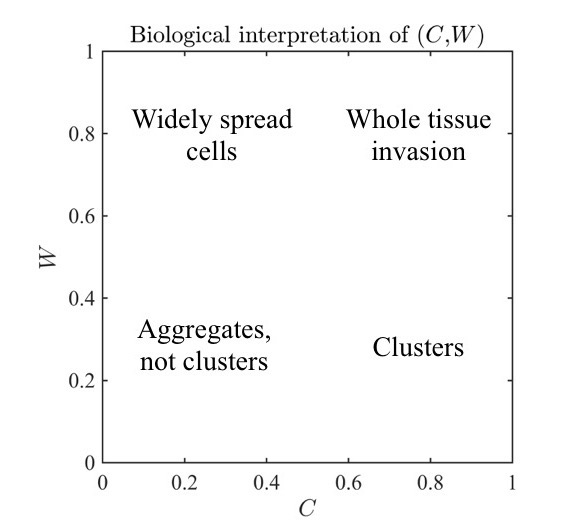
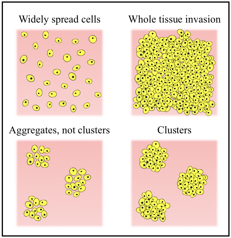
Figure 3: Biological interpretation of possible combinations of cluster width $W$ (20) and cluster compactness $C$ (21): high $W$ and low $C$ capture the scenario in which few cells are widely spread across the domain (top left region of the $C$-$W$ plane); low $W$ and low $C$ capture the presence of loose cell aggregates, (bottom left region); low $W$ and high $C$ capture the presence of clusters (bottom right region); high $W$ and high $C$ capture the scenario in which many cells are widely spread across the domain, corresponding to the case of tissue invasion in which no clusters can be identified (top right region).

3 Results

As outlined in Section 1.3, we here investigate the determinants of cluster formation and cluster size, by means of a linear stability analysis and numerical simulations, thank to which we provide an overview potential model behaviours under one-at-a-time perturbations from the baseline parameter set. We report in Section 3.1 the key results of the LSA, as described in Section 2.3, and in Sections 3.2-3.5 the results of the numerical simulations obtained using the method described in Section 2.4. In Section 3.2 we report the results of the 1D model under the baseline parameter set in Table 1 and qualitatively investigate the determinants of cluster formation in Section 3.3. In Section 3.4 we report the results of the parametric analysis conducted to elucidate the relation between different parameters and the average cluster width and compactness, as defined in Section 2.5. Finally, we report the results of the 2D model in Section 3.5.

3.1 Linear stability analysis results

We first conducted a LSA on the biologically significant spatially homogeneous steady states of the system (15) under definitions (5)-(9) and (16), both in 1D and 2D. Then, we investigated any changes in the LSA results in the absence of volume exclusion in the chemotactic and cell adhesion terms of equation (15)₁, that is under definition (17) for $f(n,\rho)$ instead of (16). The full LSA can be found in Section S1 of the supplementary document ‘SuppInfo’ with the key results being as follows. We find that the two spatially homogeneous steady states are such that either the whole domain is solely occupied by cells ($\bar{n}=1$ and $\bar{\rho}=0$) or solely occupied by ECM ($\bar{n}=0$ and $\bar{\rho}=1$), the latter of which we do not consider further as it is not biologically relevant for our current study. In absence of ECM degradation ($\gamma=0$), in addition to the two above, there are infinitely many “intermediate” spatially homogeneous steady states satisfying $0<\bar{n},\bar{\rho}<1$, with $\bar{n}+\bar{\rho}=1$. These “intermediate” steady states are linearly stable to small spatially inhomogeneous perturbations. When we neglect the influence of volume exclusion in the chemotactic and cell adhesion terms of equation (15)₁, we find that chemotaxis and cell-to-cell adhesion can combine to make the biologically significant steady states ($n>0$), which are the same as in the presence of volume exclusion, unstable to small spatially inhomogeneous perturbations if the cell density is sufficiently large (see the ‘SuppInfo’ document for more details). Thus we expect patterns to arise when cell-to-cell adhesions and chemotactic mechanisms dominate the dynamics, which may occur, for instance, when the domain is not densely packed with cells and ECM. We therefore take the initial ECM density in (13) to be $\rho_{0}=0.5$ in our nondimensional baseline parameter set, in order to increase the chances that clusters form in the model.

3.2 Cluster formation under the baseline parameter set

We report in Figure 4 the cell density $n(t,x)$ obtained from numerical simulations of the 1D model under the baseline parameter set and in Figure 5 the corresponding cluster width $W$ and compactness $C$. The plots displayed in these figures indicate that our model predicts three stages of cluster formation in 1D. First EPCs form aggregates which reach minimum cluster width of about $W=0.2$ around $t=17$ (cf. left panel in Figure 4 and Figure 5). Then the cells in these aggregates continue to proliferate increasing their compactness while keeping the cluster width unchanged up to about $t=50$ (cf. central panel in Figure 4 and Figure 5). Finally, the cells continue to proliferate until the whole domain is occupied by cells (cf. right panel in Figure 4 and Figure 5).

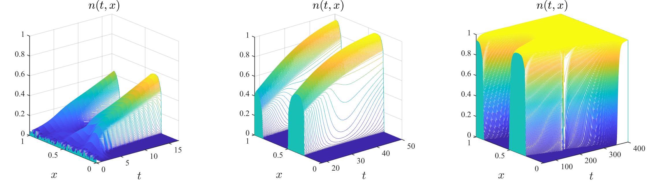
Figure 4: Plots of the cell density $n(t,x)$ obtained solving the system (15), together with definitions (5), (8) and (16), initial conditions (13) and (14)₁, complemented with zero-flux boundary conditions, under the baseline parameter set in Table 1. The solution is plotted in the time intervals $t=[0,17]$ (left panel), $t=[17,50]$ (central panel) and $t=[50,400]$ (right panel).

The simulated dynamics of cluster formation nicely match the experimentally observed ones by Blatchley et al. [16], see Figure 1, although in our simulations they occur on a slightly slower timescale. In fact in [16] the minimum cluster size was reached around 24 hours (about nondimensional time $t=8.7$) and kept unchanged while clusters increased compactness up to 48 hours ($t=17.3$) before late stage dynamics kick in. The numerically obtained cluster width corresponds to about $200\,\mu$m, which is within the range of cluster diameters observed in [16]. Finally, after $t=50$ we observe the equivalent of whole tissue invasion, suggesting our modelling framework cannot properly capture cluster stabilisation in the long run, at least in the 1D case.

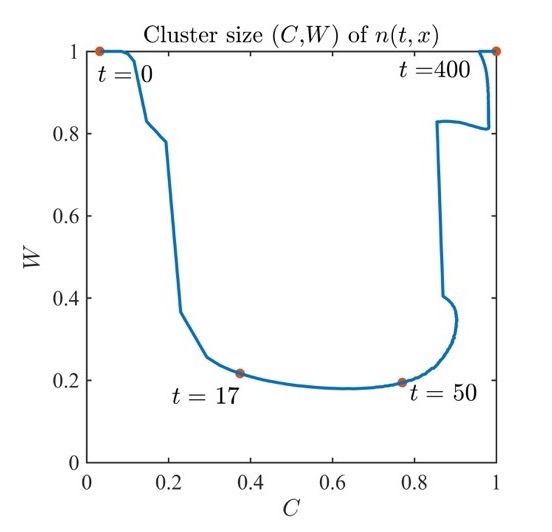
Figure 5: Average cluster width $W$ (20) and cluster compactness $C$ (21) (left panel) measured over time on the cell density $n(t,x)$ (right panel) obtained solving the system (15), together with definitions (5), (8) and (16), initial conditions (13) and (14)₁, complemented with zero-flux boundary conditions, under the baseline parameter set in Table 1, reported in Figure 4.

3.3 Qualitative investigation of the determinants of cluster formation

In view of the results reported in Section 3.2, we now investigate the role played by chemotaxis, ECM degradation and cell-to-cell adhesion in cluster formation by varying the relevant parameter values and observing changes in the solution up until $t=50$, starting from the same initial conditions considered in the previous section. The long-time dynamics (up to $t=400$) of the solutions plot in Figure 6 are reported in the supplementary Figure S2.

The primary role of chemotaxis and ECM degradation

The plots reported in the second row of Figure 6 reveal the role of chemotaxis and ECM degradation in cluster formation, according to the dynamics described in Section 2.1. Under the baseline parameter set we observe cluster formation (cf. first plot in second row of Figure 6), as discussed in the previous paragraph and summarised in Figure 4. In absence of ECM degradation, even though cell aggregates of the same width form, the maximum cell density remains below $0.3$ (cf. second plot in second row of Figure 6) and actually decays over longer periods of time (see supplementary Figure S2). On the other hand, in absence of chemotaxis no cell aggregation occurs and we either observe total invasion of the domain by the cells (cf. third plot in second row of Figure 6) or, in absence of ECM degradation, a simple spatial redistribution of the cells (cf. fourth plot in second row of Figure 6). These results indicate that chemotaxis and ECM degradation are both crucial to cluster formation, with chemotaxis playing a key role in cell aggregation and ECM degradation being responsible for these aggregates to grow into well-defined and compact clusters.

The secondary role of cell-to-cell adhesion

Let us now compare the plots in the second row of Figure 6 with those in the rest of the figure, which have been obtained by varying the cell-to-cell adhesion coefficient $S_{nn}$, the value of which was chosen a priori due to lack of proper estimates in the current literature. We immediately observe that for small values $S_{nn}\leq 0.1$, under the baseline parameter set, cell-to-cell adhesion does not play any particular role in cluster formation, as demonstrated by the fact that the simulations in absence of cell-to-cell adhesion closely resemble those with $S_{nn}=0.1$ (cf. first and second row of Figure 6 and Figure S3 in ‘SuppInfo’ document). On the other hand, increasing the order of magnitude of the cell-to-cell adhesion coefficient results in the initial formation of small-scale aggregates. Moreover, the maximum density reached by these aggregates increases as $S_{nn}$ increases (cf. third and fourth row of Figure 6). This however does not seem to affect the long-time dynamics of the solution, which remain analogous to those described in the previous paragraph. For instance, under the baseline parameter set except for $S_{nn}=1$, the initial aggregates merge – likely due to chemotaxis – into wider clusters and then proceed to invade the whole tissue (cf. first plot in third row of Figure 6 and of Figure S2). For $S_{nn}=10$ we do not yet observe small aggregates merging into larger clusters at $t=50$ – likely due to cell-to-cell adhesion overpowering chemotaxis – and tissue invasion is simply delayed (cf. first plot in fourth row of Figure 6 and of Figure S2). Overall these results suggest that the continuum nonlocal description of cell-to-cell adhesion considered in our model, while it may capture the aggregating effect of cell-to-cell adhesion for $S_{nn}$ high enough, does not capture the stabilising effect that we are seeking for in this modelling framework.

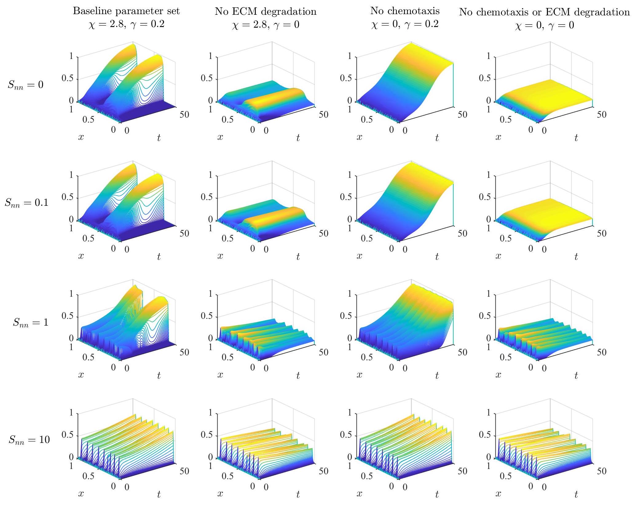
Figure 6: First row: Plots of the cell density $n(t,x)$ up to $t=50$ obtained solving the system (15), together with definitions (5), (8) and (16), initial conditions (13) and (14)₁, complemented with zero-flux boundary conditions, in absence of cell-to-cell adhesion, i.e for $S_{nn}=0$: under the baseline parameter set (first column), in absence of ECM degradation, i.e. for $\gamma=0$ (second column), in absence of chemotaxis, i.e. $\chi=0$ (third column), and in absence of both chemotaxis and ECM degradation, i.e. $\chi=\gamma=0$ (fourth column). Second, third and fourth rows: Same as first row but in the presence of cell-to-cell adhesion, with $S_{nn}=0.1$ (second row), $S_{nn}=1$ (third row) and $S_{nn}=10$ (fourth row) respectively.

3.4 Quantitative investigation of the determinants of cluster size

We study changes in the measures $W$ and $C$, defined according to (20) and (21), at $t=50$ under variations of each parameter in the baseline parameter set. In particular, we consider the effect of halving and doubling the magnitude of each parameter in equations (15)₁ and (15)₂ in Figure 7, and those in equations (15)₃ and (15)₄ in Figure 8. Each boxplot had been obtained using data from 100 simulations under the same parameter set, staring from randomised initial conditions as in (13) and (14)₁.

The cluster width $W$ measured over 100 simulations under the baseline parameter width ranges between $0.15$ and $0.41$ with median (and mean) around $0.23$, as portrayed in Figures 7 and 8 (central boxplot in each $W$ plot). The nondimensional width corresponds to a diameter in the range $150-410\mu$m, which is consistent with the experimentally observed cluster sizes in [16] (cf. Figure 1).

The role of chemotaxis

Boxplots of the width $W$ and compactness $C$ of clusters for different values of the chemotactic sensitivity $\chi$ are displayed in Figure 7b. While higher values of $\chi$ correlate with slightly smaller clusters, yet maintaining a mean width around 0.2, lowering the magnitude of $\chi$ seems to result in a wider range of values of $W$ with much higher median, as well as higher compactness $C$. This supports the notion that lowering the chemotactic sensitivity of the cells hinders cluster formation and – assuming all other dynamics are present – fosters tissue invasion, which is in line with the results presented in Section 3.3.

The role of ECM degradation

Boxplots of the width $W$ and compactness $C$ of clusters for different values of the ECM degradation rate $\gamma$ are displayed in Figure 7f. Notice that, while the median width $W$ is maintained around 0.2, increasing the magnitude of $\gamma$ results in a smaller range of values measured for both $W$ and $C$, as well as higher values of cluster compactness. In addition, this trend suggests that further decreasing $\gamma$ will lead to higher values of $W$ and lower values of $C$ measured (see supplementary Figure S4c in ‘SuppInfo’ document), which is in line with the observed dynamics in absence of ECM degradation in Section 3.3 (cf. Figure 6, second and fourth columns). Overall, this highlights the key role ECM degradation has in cluster formation, establishing a relation between the rate $\gamma$ and the cluster compactness $C$.

The role of matrix remodelling

We see in Figure 7g that increasing the magnitude of the matrix remodelling rate $\mu$ results in a larger range of values measured for both $W$ and $C$, as well as lower values of cluster compactness, while the median width $W$ is maintained around 0.2. These are opposite effects to those obtained increasing its degradation rate $\gamma$ (vid. Figure 7f), which is coherent with the opposite nature of these dynamics.

The role of cell-to-cell adhesion

The plots in Figure 7c confirm that small variations in the cell-to-cell adhesion coefficient $S_{nn}$ do not influence the size of clusters, as expected from the results in Section 3.3. Additional numerical tests considering different orders of magnitude of $S_{nn}$ (see supplementary Figure S1b in ‘SuppInfo’ document) revealed a slight increase in the median $W$, probably due to the initial presence of smaller clusters (cf. Figure 6, third row) which at $t=50$ may still be in the process of merging depending on their spatial distribution. These results do not suggest that cell-to-cell adhesion is a key mechanism in determining cluster – and therefore network – topology.

The role of cell diffusion and cell-matrix interactions

The boxplots of $W$ and $C$ of clusters for different values of the cell diffusion coefficient $D_{n}$, displayed in Figure 7a, show that changing the magnitude of $D_{n}$ has very little effect on the cluster compactness $C$ and median width $W$. There is however an increasing range of values of $W$ measured as $D_{n}$ increases, indicating that low diffusivity correlates with more precisely defined clusters, while high diffusivity results in more variability in cluster size. Moreover, this variability allows for larger values of $W$ to be measured, suggesting that much higher diffusivity may result in tissue invasion (see supplementary Figure S4a in ‘SuppInfo’ document). The same observations can be conducted on the boxplots in Figure 7d, obtained by varying the magnitude of the cell-to-matrix adhesion coefficient. This is in line with the notion that lower cell-matrix interactions facilitate cluster formation, while much higher cell-matrix interactions promote tissue invasion.

The role of cell proliferation

In Figure 7e we see that slower proliferation – i.e. lower $p$ – correlates with a wide range of lower values of cluster compactness $C$ measured, while the median width is maintained around 0.2. On the other hand, faster proliferation – i.e. higher $p$ – results in a wide range of higher values of cluster width $W$ and a small range of high values of compactness $C$. Note that these data portray different stages of the cluster formation process, as demonstrated in Figure 5 (central panel): initially aggregates form without being very condensed (low-to-medium $W$ and $C$), then they increase their compactness while keeping steady width (low $W$ and high $C$), and eventually grow further invading the surrounding space (medium-to-high $W$ and high $C$). This suggests that the rate of proliferation of EPCs might play a key role in determining the speed of the cluster formation process.

The role of initial ECM density

The plots in Figure 7h indicate that changes in the initial ECM density $\rho_{0}$ does not affect the long-time spatio-temporal dynamics. In fact, while different values of $\rho_{0}$ results in slightly different values of the median width and compactness of clusters observed at $t=50$, these values still capture the same biological scenario (i.e. cluster are recognisable at $t=50$).

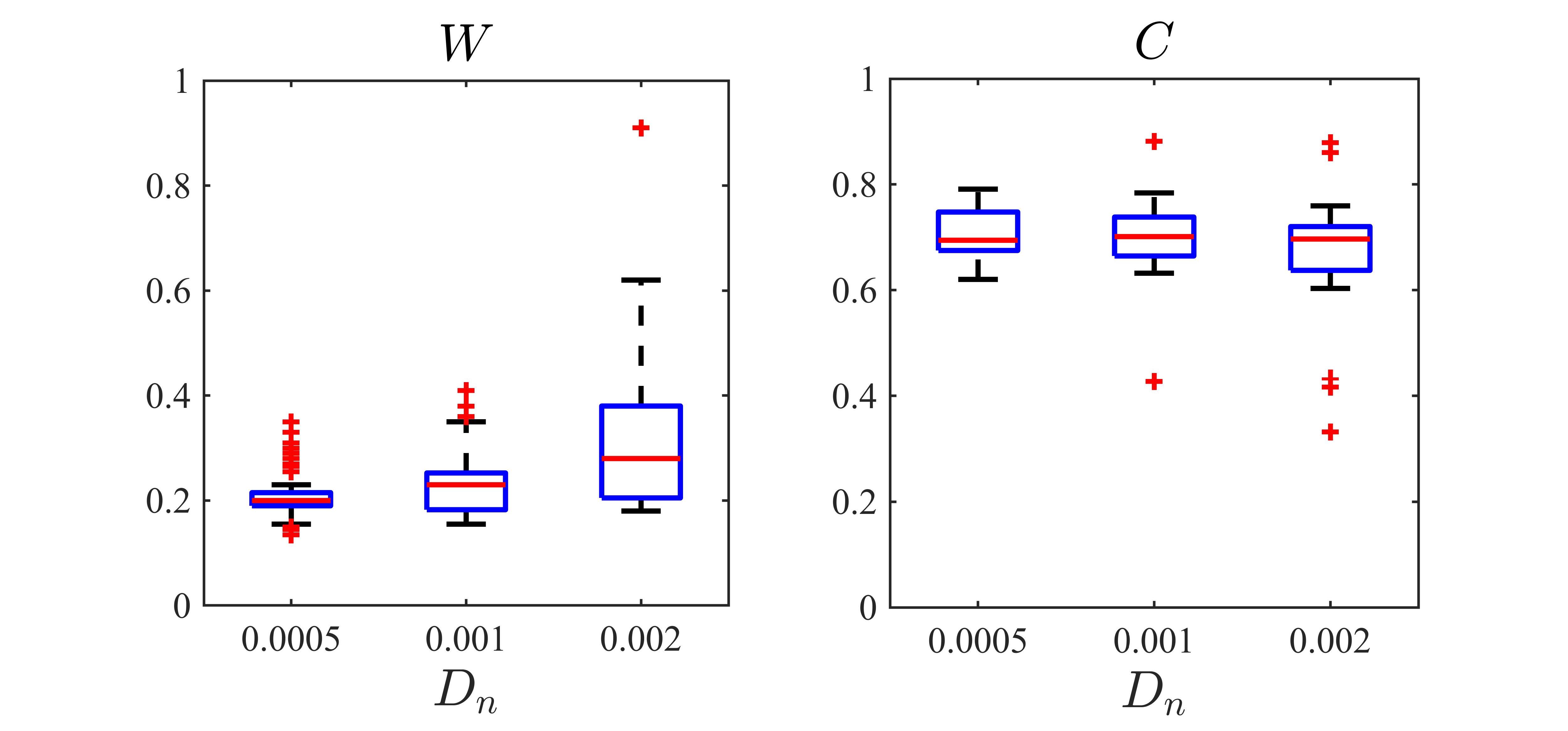
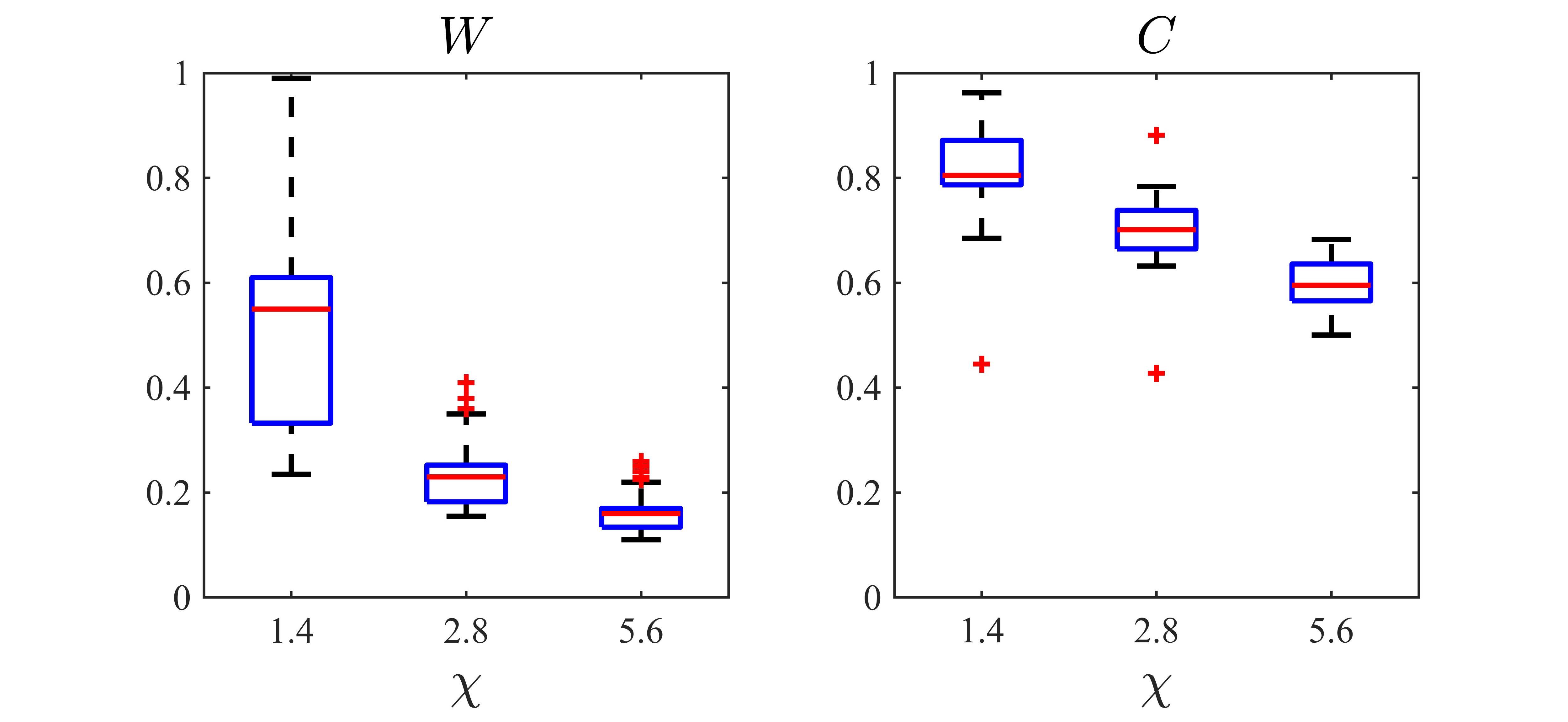
(a) Varying cell diffusion $D_{n}$

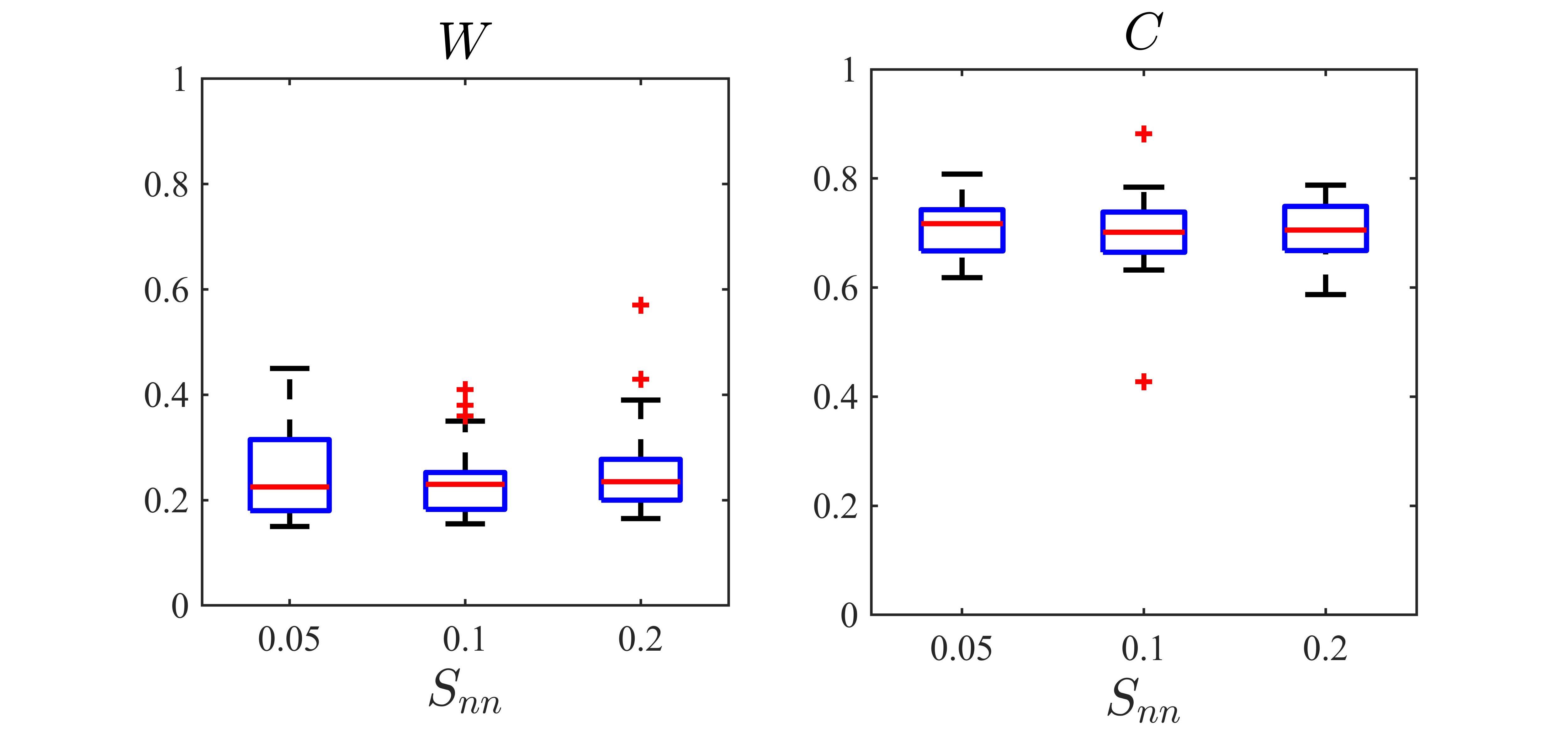
(b) Varying chemotactic sensitivity $\chi$

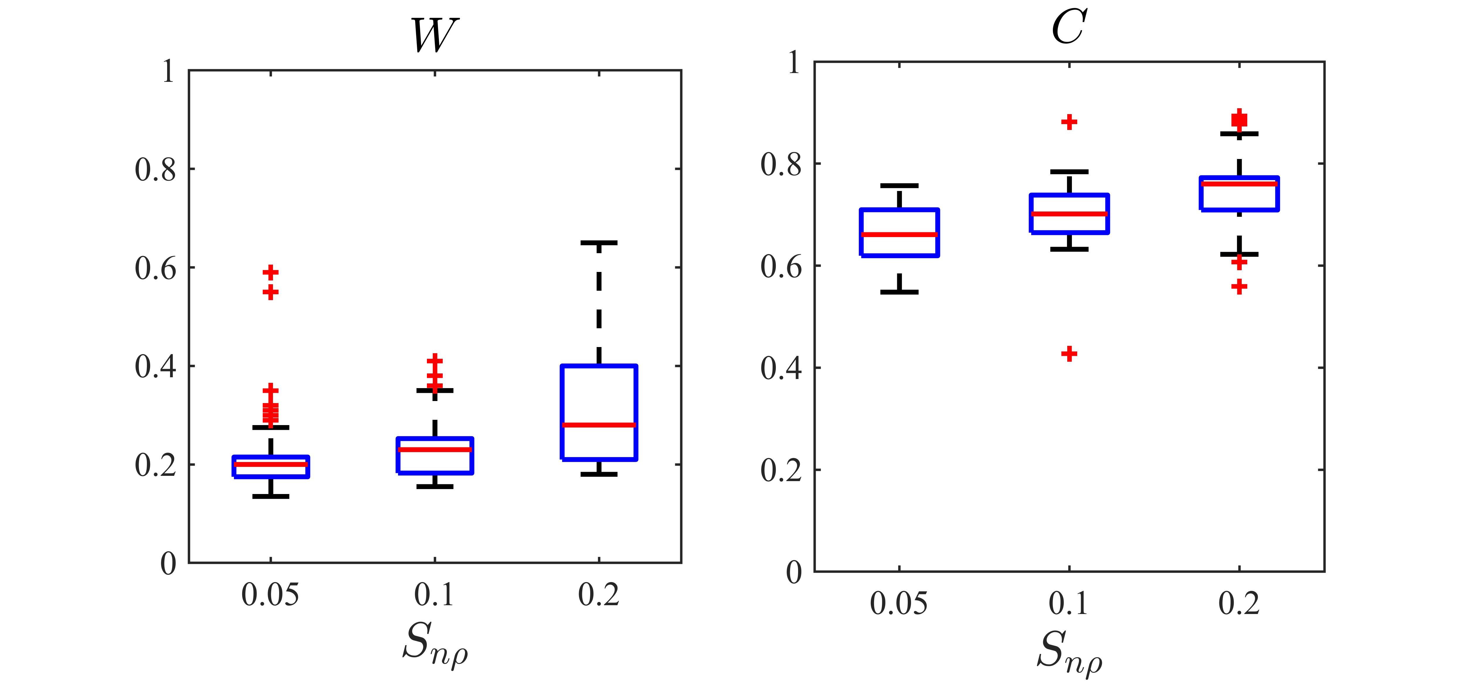
(c) Varying cell-to-cell adhesion coefficient $S_{nn}$

(d) Varying cell-to-matrix adhesion coefficient $S_{n\rho}$

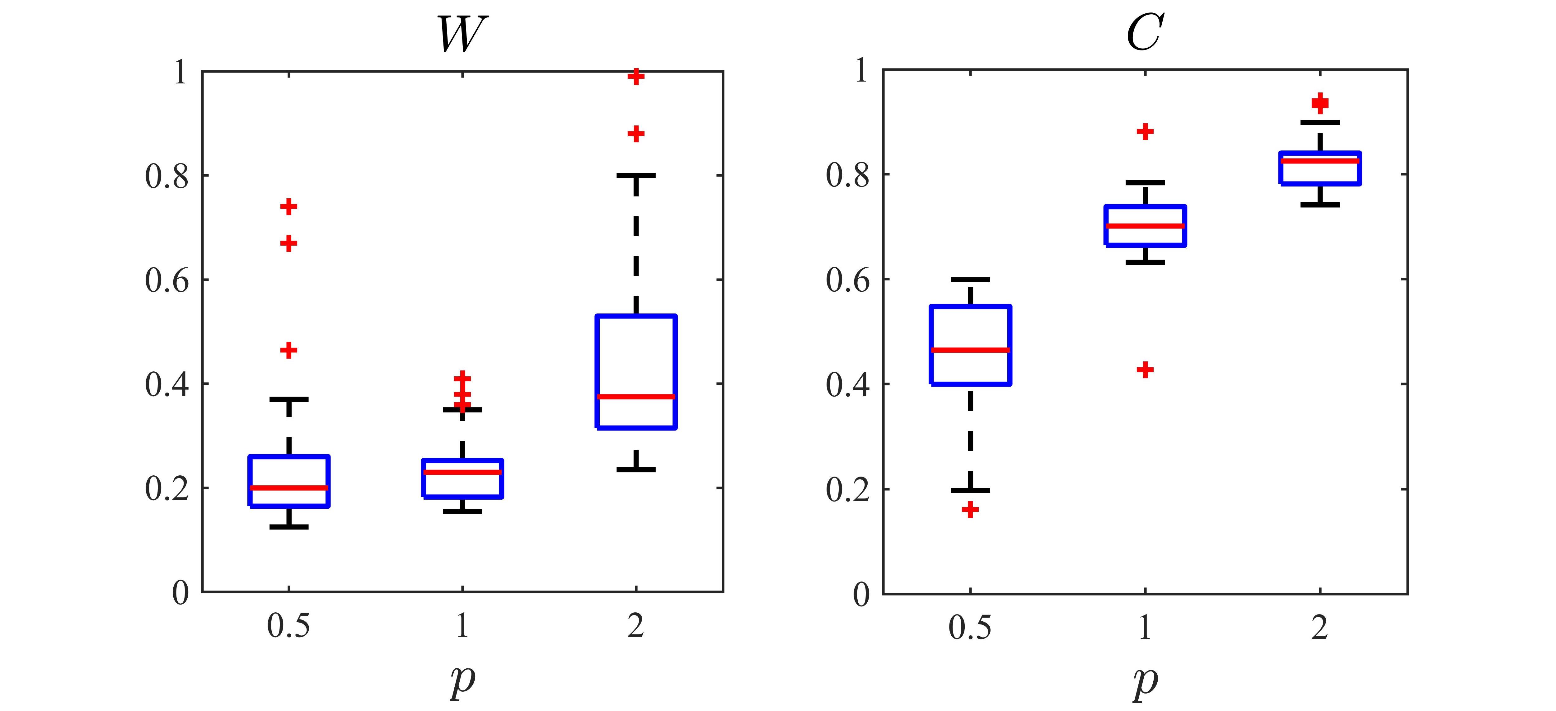
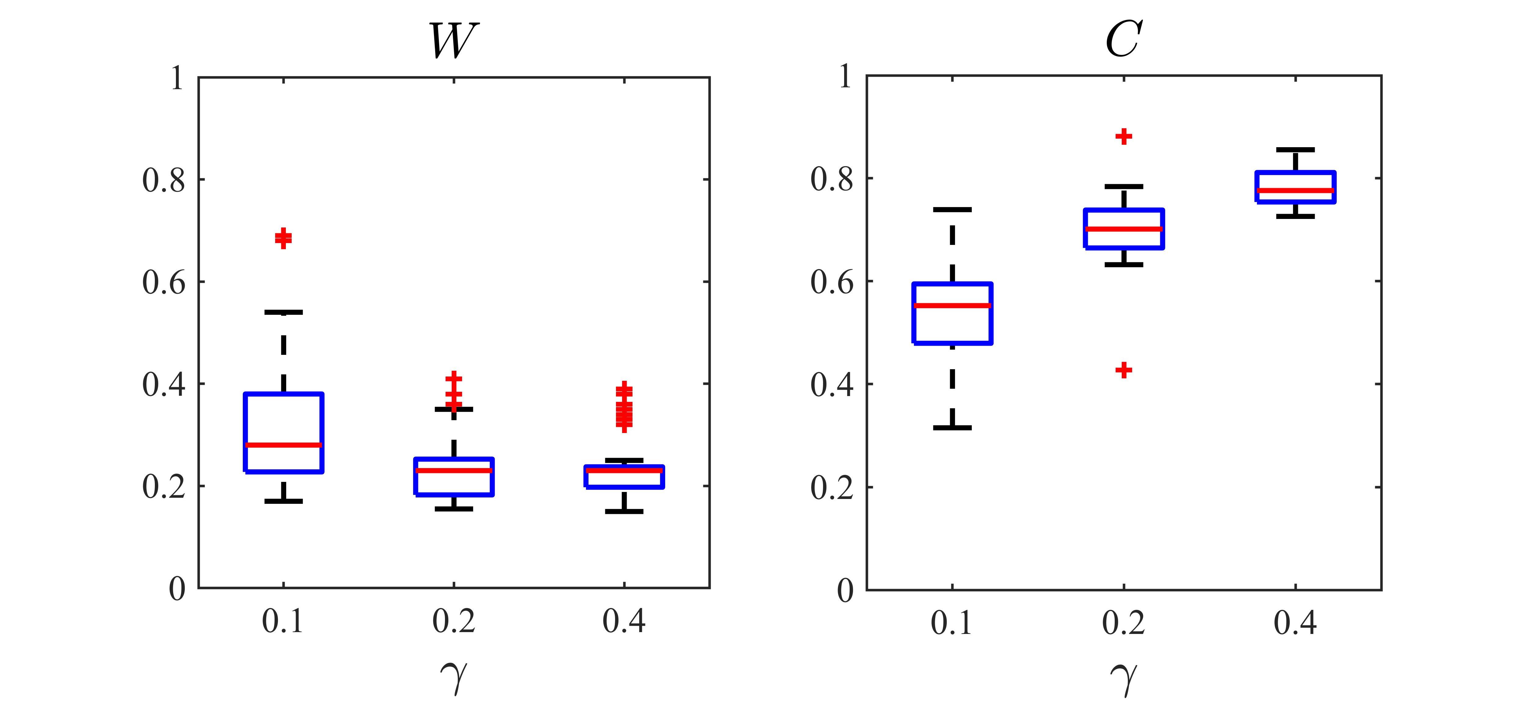
(e) Varying cell proliferation rate $p$

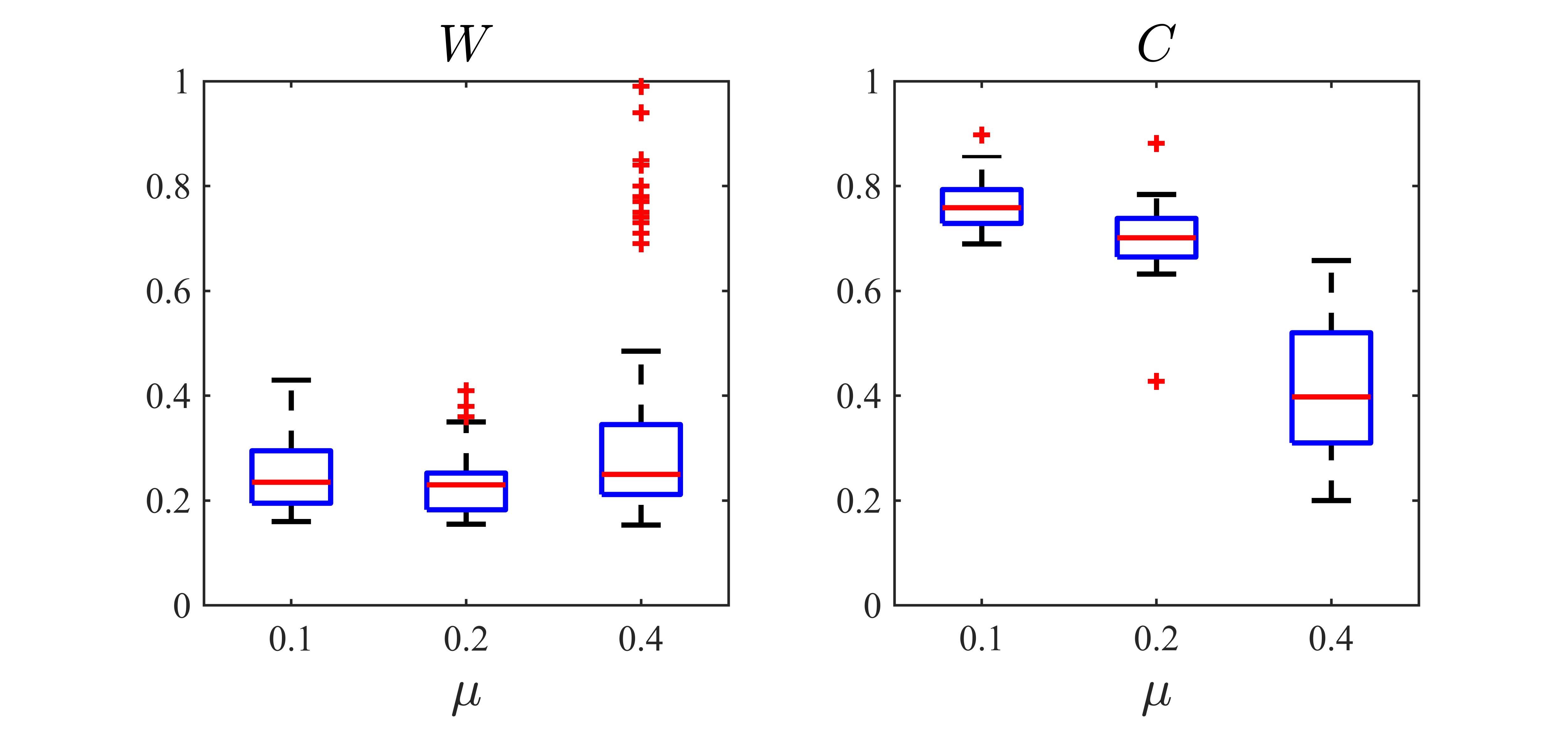
(f) Varying ECM degradation rate $\gamma$

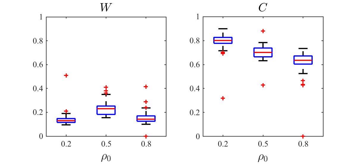
(g) Varying ECM remodelling rate $\mu$

(h) Varying initial ECM density $\rho_{0}$

Figure 7: Cluster width $W$ and compactness $C$, defined in (20) and (21), under variations from the baseline parameter set (BPS), in Table 1, of each parameter in equations (15)₁ and (15)₂. In (a) we have boxplots of $W$ and $C$ measured on the numerical solution of the system (15) at $t=50$, for $D_{n}$ taking its value in the BPS (center), half (left) and double (right) its value in the BPS. Each boxplot collects data from 100 simulations under randomised initial conditions (13)-(14)₁. In (b)-(g) we have the same as in (a) but varying parameters $\chi$ (b), $S_{nn}$ (c), $S_{n\rho}$ (d), $p$ (e), $\gamma$ (f), $\mu$ (g) and $\rho_{0}$ (h).

The role of VEGFs dynamics

Figure 8e displays changes in cluster width $W$ and compactness $C$ as the rate production of VEGFs $\alpha_{c}$ varies. Note that these results well mirror those obtained by varying chemotactic sensitivity (cf. Figures 7b and 8e), which is coherent with the notion that higher VEGF production rates correlate with stronger chemotactic dynamics, already established to play a key role in cluster formation. In addition, the size of clusters seems to be proportional to the VEGF diffusion coefficient $D_{c}$, as demonstrated by the plots in Figure 8d in which we see that increasing the magnitude of $D_{c}$ results in higher $W$ and $C$. This trend, however, suggests that much higher values of $D_{c}$ may result in tissue invasion, rather than cluster formation (see supplementary Figure S4e in ‘SuppInfo’ document). Finally, as suggested by Figure 8f, changes in the VEGF decay rate $\lambda_{c}$ do not seem to particularly effect cluster size over the range of parameter values considered.

The role of MMPs dynamics

Figure 8b displays changes in cluster width $W$ and compactness $C$ as the rate production of MMPs $\alpha_{m}$ varies. Similarly to what was observed for $\alpha_{c}$ in relation to $\chi$, we see that these boxplots closely resemble those obtained varying $\gamma$ (cf. Figures 7f and 8b), which is coherent with the notion that higher MMP production rates correlate with stronger degrading dynamics, already established to be responsible for turning aggregates into clusters – that is, increasing their compactness. In addition, we see in Figure 8c that increasing the magnitude of the MMPs decay rate $\lambda_{m}$ yields opposite effects to those obtained increasing their production $\alpha_{m}$, further confirming the role MMP-mediated ECM degradation has in cluster formation. On the other hand, changes in the MMPs diffusivity $D_{m}$ do not seem to affect cluster size, as demonstrated in Figure 8a – verified under different orders of magnitude of $D_{m}$ (see supplementary Figure S4d in ‘SuppInfo’ document). This suggests not much will be gained by distinguishing between membrane-bound and diffusive MMPs, at least in this modelling framework and within the range of parameter values considered.

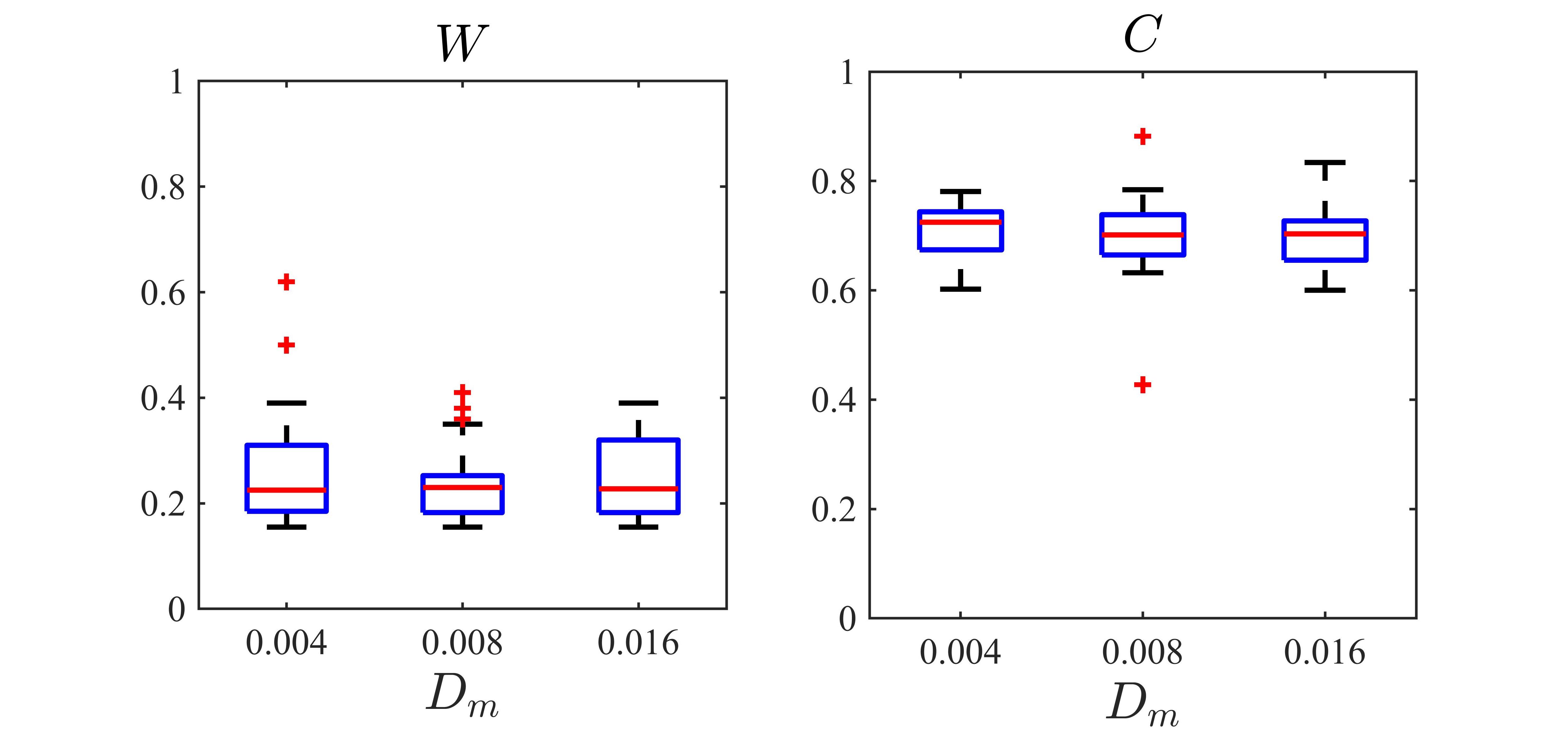
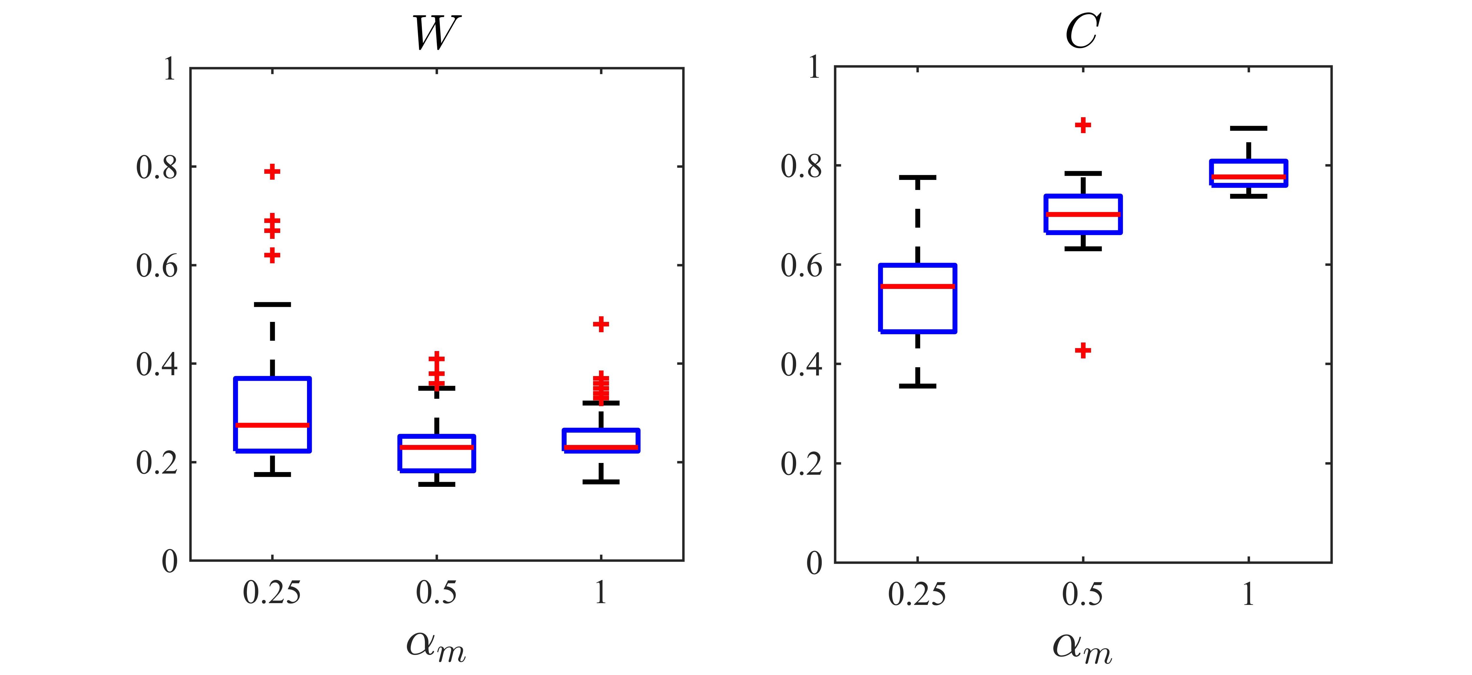
(a) Varying MMP diffusion $D_{m}$

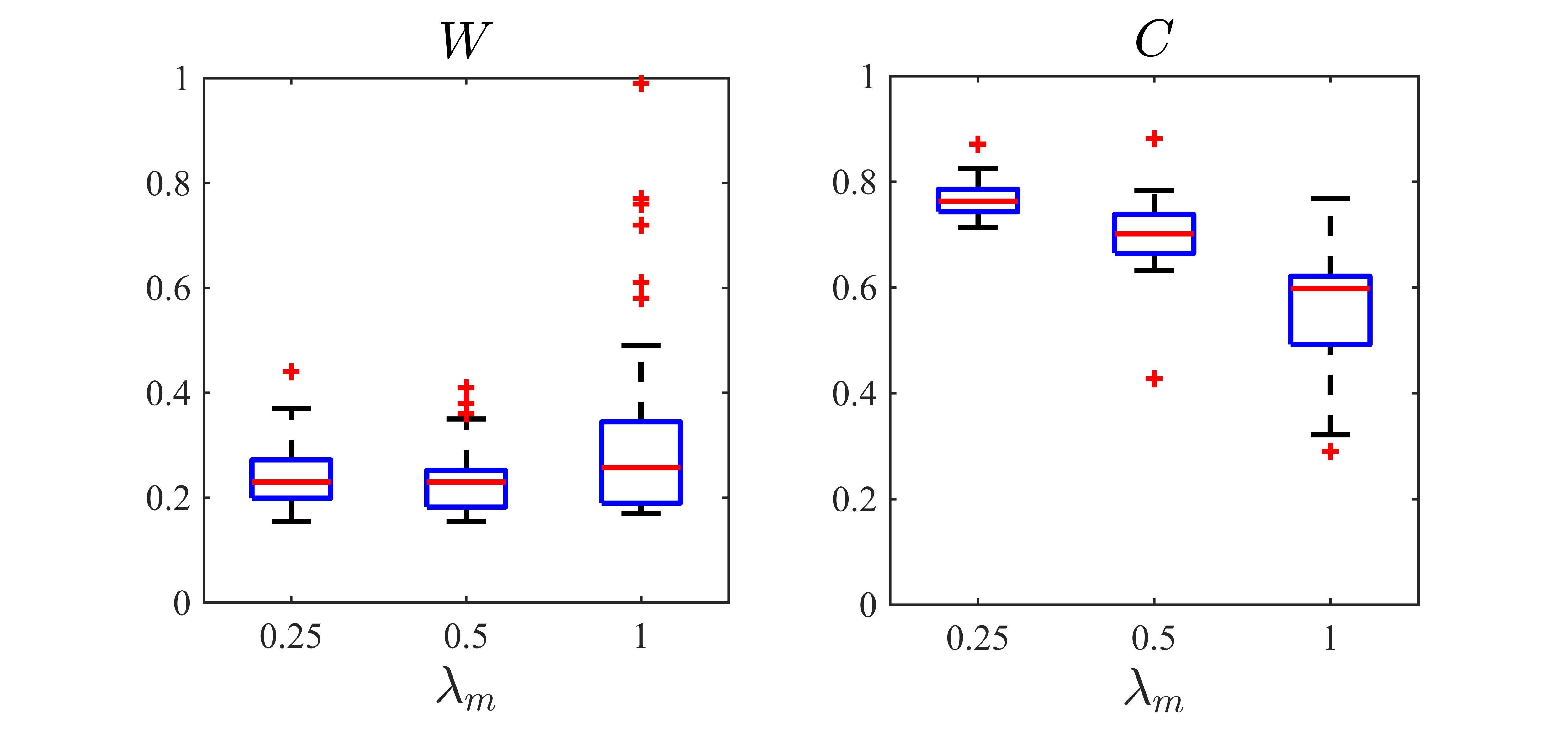
(b) Varying MMP production rate $\alpha_{m}$

(c) Varying MMP decay rate $\lambda_{m}$

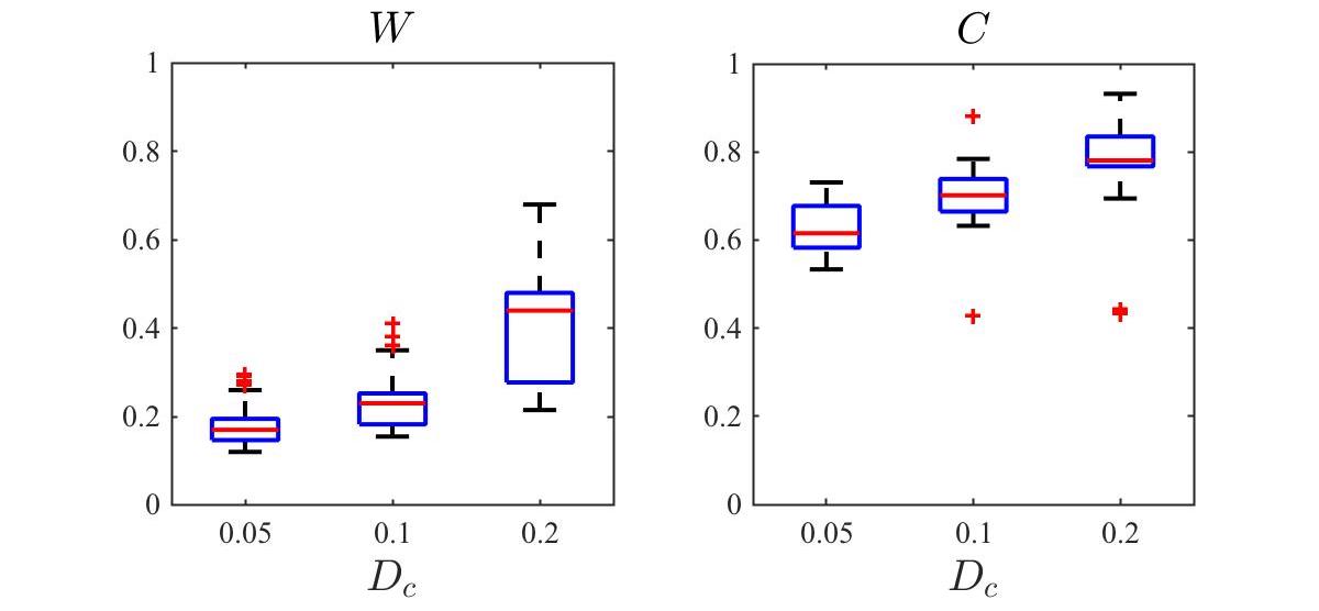
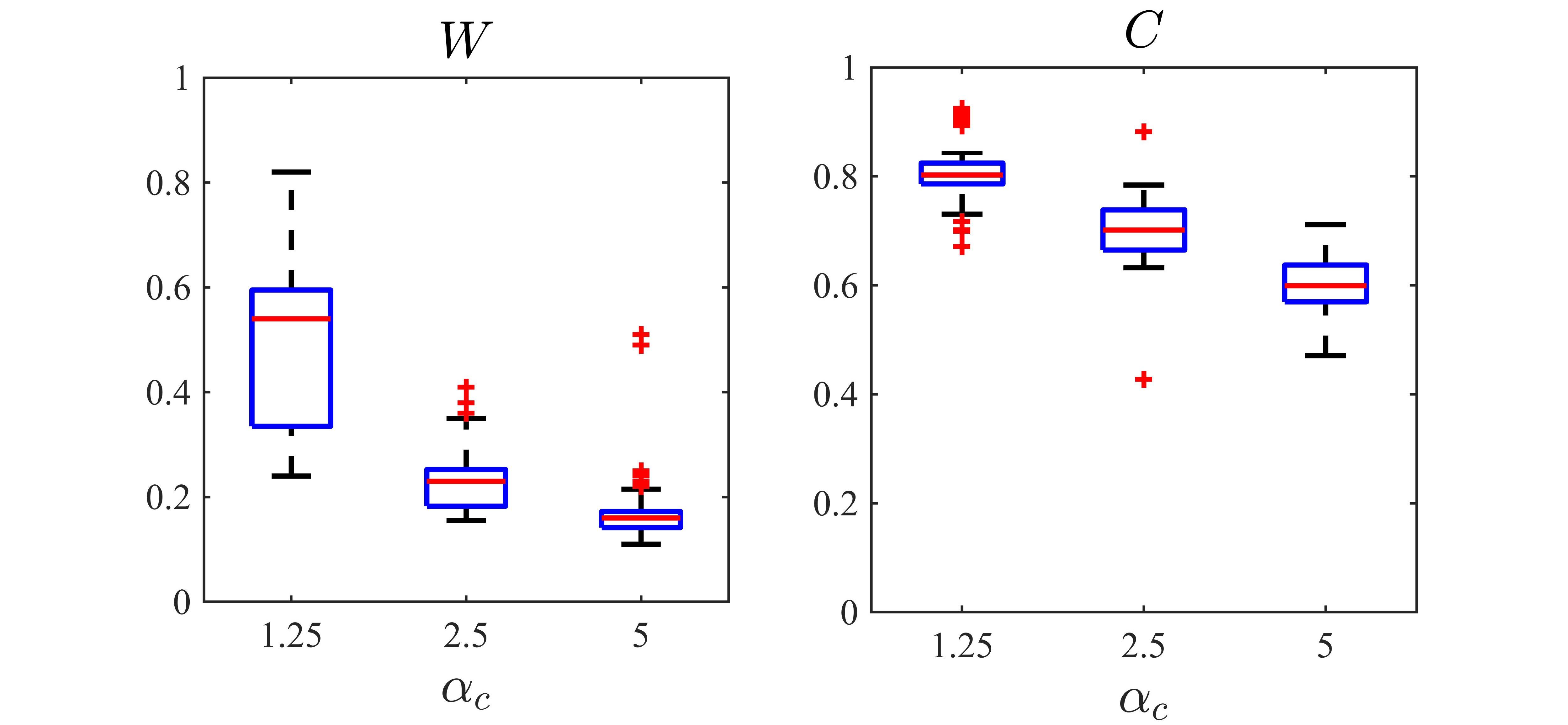
(d) Varying VEGF diffusion $D_{c}$

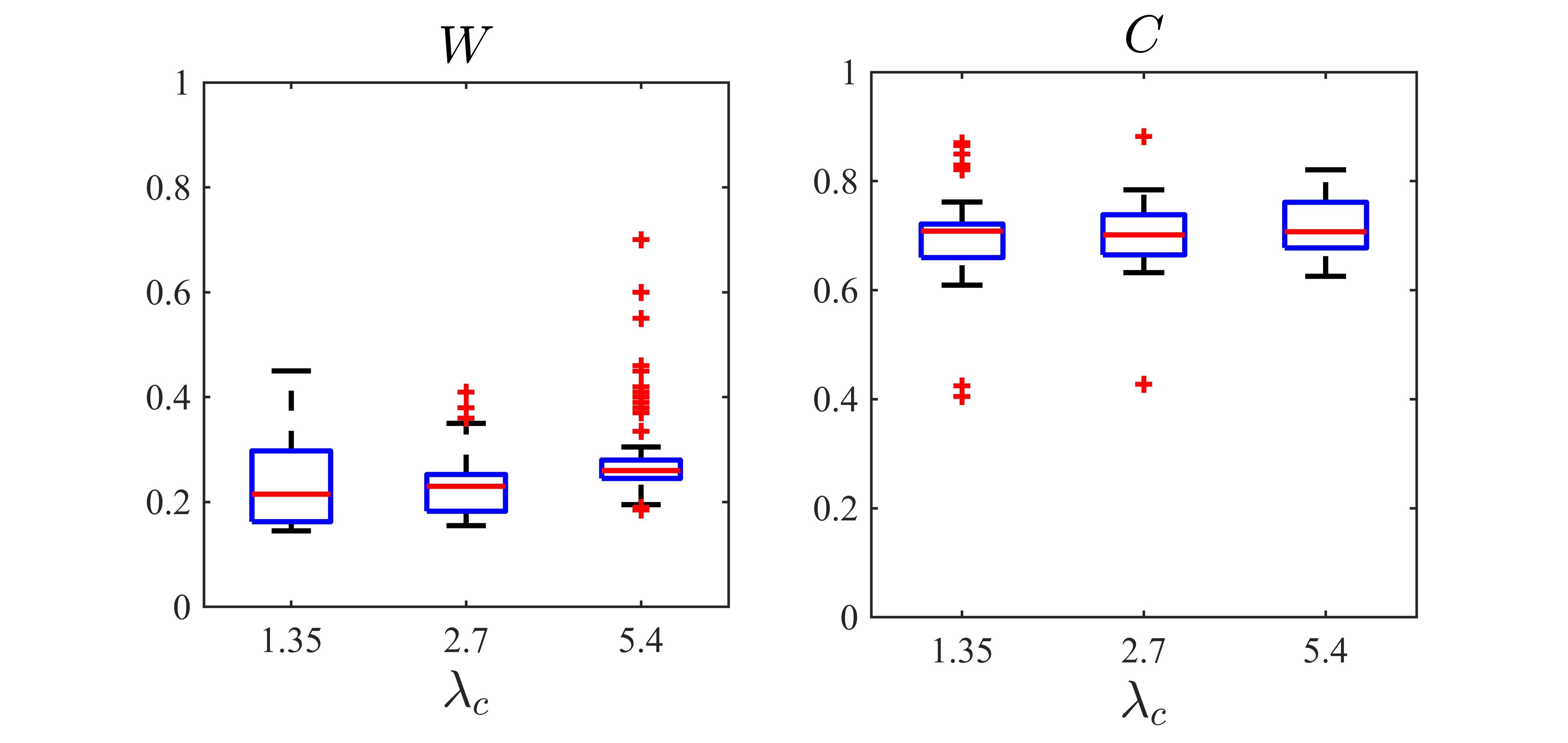
(e) Varying VEGF production rate $\alpha_{c}$

(f) Varying VEGF decay rate $\lambda_{c}$

Figure 8: Cluster width $W$ and compactness $C$, defined in (20) and (21), under variations from the baseline parameter set in Table 1 of each parameter in equations (15)₃ and (15)₄. In (a) we have boxplots of $W$ and $C$ measured on the numerical solution of the system (15) at $t=50$, for $D_{m}$ taking its value in the BPS (center), half (left) and double (right) its value in the BPS. Each boxplot collects data from 100 simulations under randomised initial conditions (13)-(14)₁. In (b)-(f) we have the same as in (a) but varying parameters $\alpha_{m}$ (b), $\lambda_{m}$ (c), $D_{c}$ (d), $\alpha_{c}$ (e) and $\lambda_{c}$ (f).

3.5 Two-dimensional clusters

Let us now consider the 2D problem. In this section we focus on the most interesting results obtained in Section 3.4 and investigate the role played by chemotaxis, ECM degradation and cell proliferation in the formation of 2D clusters. We also consider the results in absence of ECM remodelling, discussing its biological interpretation in relation to in vitro and in vivo assays.

2D clusters under the baseline parameter set

Under the baseline parameter set reported in Table 1, 2D cluster formation follows slightly different spatio-temporal dynamics to those observed in the 1D case, as demonstrated by the plots in the second row of Figures 9, 10 and 11. At $t=20$ the cell density has already reached maximum local compactness in some regions, while aggregation dynamics are still at their early stages (cf. first panel in second row of Figures 9, 10 or 11), and the minimum cluster size is observed no earlier than $t=140$ (cf. fourth panel in second row of Figures 9, 10 or 11). The cluster observed at this stage has a nondimensional diameter of about 0.2, which agrees with the results in 1D and is therefore also consistent with experimental observations reported by Blatchley et al. [16]. After the cluster has formed, no tissue invasion is observed – see supplementary Figure S5 in ‘SuppInfo’ document.

The role of ECM degradation in 2D

The plots reported in Figure 9 demonstrate that ECM degradation promotes the formation of 2D clusters, as predicted by the results of the 1D model presented in Sections 3.3 and 3.4. Lower ECM degradation rates correlate with slower aggregation dynamics and lower compactness of such aggregates (cf. first row of Figure 9) – to the extent that in absence of ECM degradation no clusters form (see supplementary Figure S6 in ‘SuppInfo’ document) – and higher ECM degradation rates correlate with faster cluster formation with well-defined and compact clusters observed at much earlier times (cf. third row of Figure 9). As for the 1D model, we obtain the same results under analogous variations of the MMP secretion rate $\alpha_{m}$ (see supplementary Figure S7 in ‘SuppInfo’ document).

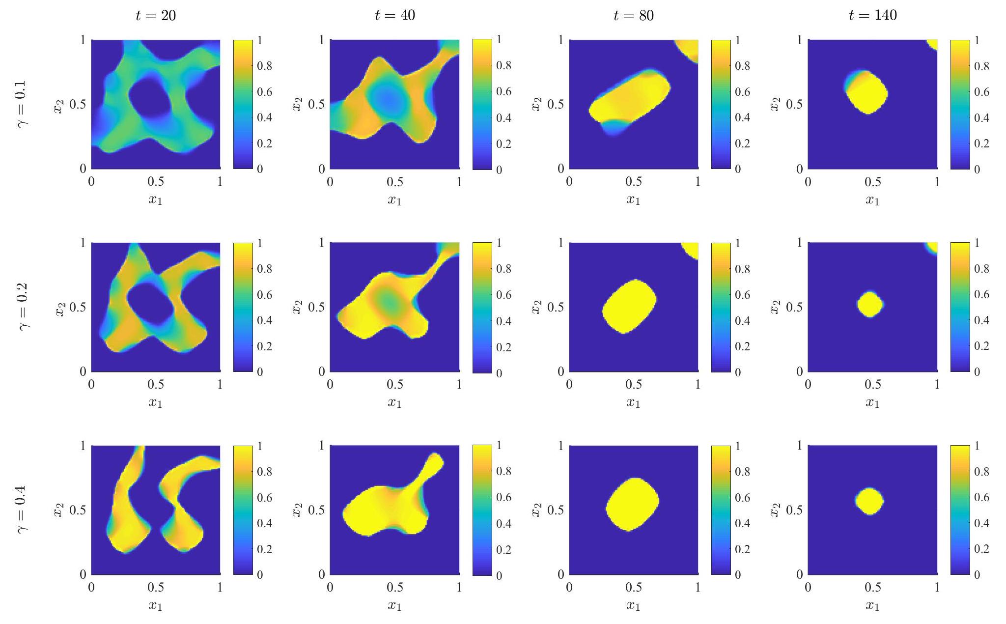
Figure 9: First row: Plots of the cell density $n(t,{\bf x})$ obtained solving the system (15), together with definitions (6), (8) and (16), initial conditions (13) and (14)₂, complemented with zero-flux boundary conditions, under the parameter choices reported in Table 1, except for $\gamma=0.02$. The solution is plotted at time $t=20$ (first panel), $t=40$ (second panel), $t=80$ (third panel) and $t=140$ (fourth panel). Second and third row: Same as first row, except for $\gamma=0.2$ (second row) and $\gamma=2$ (third row).

The role of chemotaxis in 2D

The plots reported in Figure 10 demonstrate that endogenous chemotaxis promotes aggregation dynamics, as predicted by the results of the 1D model presented in Sections 3.3 and 3.4, and reveal that chemotaxis is an important determinant of 2D cluster topology. Lower values of the chemotactic sensitivity $\chi$ correlate with slower and weaker aggregation dynamics, so that no well-defined clusters can be observed (cf. first row of Figure 10). Higher values of $\chi$ correlate with faster and stronger aggregation dynamics, with well-defined clusters observed at earlier times (cf. third row of Figure 10) and cluster diameter – once the clusters have reached minimum size – smaller than that observed with lower values of $\chi$ (cf. last panel in the second row and last panel in the third row of Figure 10). As for the 1D model, we obtain the same results under analogous variations of the VEGF secretion rate $\alpha_{c}$ (see supplementary Figure S8 in ‘SuppInfo’ document).

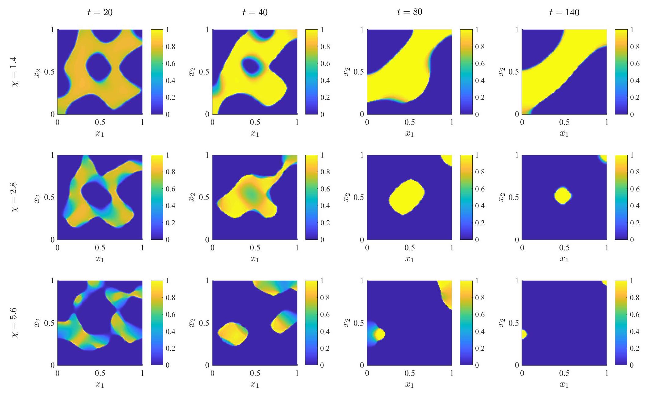
Figure 10: First row: Plots of the cell density $n(t,{\bf x})$ obtained solving the system (15), together with definitions (6), (8) and (16), initial conditions (13) and (14)₂, complemented with zero-flux boundary conditions, under the parameter choices reported in Table 1, except for $\chi=1.4$. The solution is plotted at time $t=20$ (first panel), $t=40$ (second panel), $t=80$ (third panel) and $t=140$ (fourth panel). Second and third row: Same as first row, except for $\chi=2.8$ (second row) and $\chi=5.6$ (third row).

The role of cell proliferation in 2D

While the results of the 1D model presented in Section 3.4 seemed to suggest that the speed of the cluster formation process is proportional to the cell proliferation rate $p$, the plots reported in Figure 11 in a 2D framework indicate otherwise. While the rate of cell proliferation may influence how the cells respond to spatial gradients at the beginning of the cluster formation process (cf. plots in the second column of Figure 11), it does not seem to affect the overall spatio-temporal dynamics of 2D cluster formation. Upon these considerations, the results displayed in Figure 7 may simply be a 1D projection of the 2D dynamics occurring around the same time – consider for instance a 1D cross section (e.g. $x_{1}=0.5$) of the plots in the second column of Figure 11.

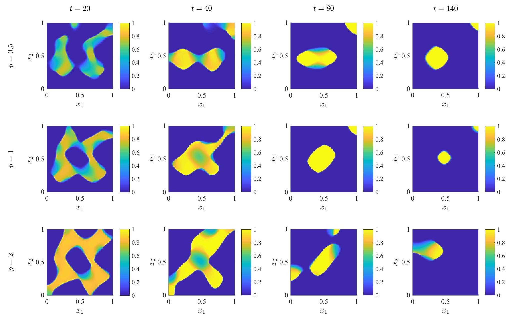
Figure 11: First row: Plots of the cell density $n(t,{\bf x})$ obtained solving the system (15), together with definitions (6), (8) and (16), initial conditions (13) and (14)₂, complemented with zero-flux boundary conditions, under the parameter choices reported in Table 1, except for $p=0.5$. The solution is plotted at time $t=20$ (first panel), $t=40$ (second panel), $t=80$ (third panel) and $t=140$ (fourth panel). Second and third row: Same as first row, except for $p=1$ (second row) and $p=2$ (third row).

The role of matrix remodelling and its relation to in vitro studies

While matrix remodelling naturally occurs in vivo thanks to the presence of other cells in biological tissue, this is not generally observed in in vitro assays, which occur in isolated environments. Thus, in order to compare our results with those of in vitro studies, we chose to set the ECM remodelling rate $\mu=0$, the results are presented in Figure 12. We observe that clusters still form in the absence of ECM remodelling, however they are smaller than in the baseline parameter set (cf. last panel in the second row of Figures 9-11 and that of Figure 12). The smaller cluster sizes may result from the more dominant role played by cell-to-cell adhesion following ECM degradation: in absence of ECM remodelling, volume exclusion is less likely to affect the cell dynamics and, at the cell boundaries, cell-matrix interactions become negligible compared to cell-cell interactions. We would then expect to observe clusters of a smaller diameter but higher maximum density, but because of death due to competition for space we instead observe a loss of cell mass. While these results are mathematically consistent with our model set up, the observed cluster size under the baseline parameter set was more coherent with in vitro experimental observations in [16] than that observed for $\mu=0$. This could be explained by considering that our 2D set up is meant to reflect dynamics occurring in a 2D horizontal cross section of the 3D experimental domain reported in [16], illustrated in Figure 1A. As the cells degraded the matrix and reorganised into clusters, they also fell towards the bottom of the hydrogel, as illustrated by the experimental data reported in Figure 13, in regions where it was not yet degraded. Thus, following the horizontal plane intersecting the cluster’s center, we would likely observe section crossing the center of a cluster, we would indeed observe cell-independent matrix remodelling.

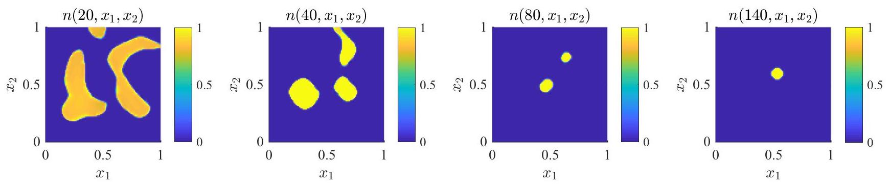
Figure 12: Plots of the cell density $n(t,{\bf x})$ obtained solving the system (15), together with definitions (6), (8) and (16), initial conditions (13) and (14)₂, complemented with zero-flux boundary conditions, under the parameter choices reported in Table 1, except for $\mu=0$. The solution is plotted at time $t=20$ (first panel), $t=40$ (second panel), $t=80$ (third panel) and $t=140$ (fourth panel).

Figure 13: Visual summary of the number of single cells (bottom) and the number of cells in clusters (top) observed over time at different heights in the 3D matrigel in hypoxic gradients by Blatchley et al. [16] – experimental set up illustrated in Figure 1A (bottom). Figure taken from Figure 1E in [16] under Creative Commons licence https://creativecommons.org/licenses/by-nc/4.0/.

4 Discussion and research perspectives

Despite the great progress made in the past 20 years in understanding the mechanisms behind EPC cluster-based vasculogenesis, much more needs to be achieved in order to unlock its full therapeutic potential. Mathematical modelling provides theoretical means to shed light on the otherwise hidden role played by underlying dynamics in the origin and structure of the emergent vascular network, as previously achieved in the study of mature EC vascular network formation (single-cell vasculogenesis). We therefore formulated a nonlocal PDE model of EPC cluster formation during the early stages of vasculogenesis, including mechanisms such as ECM degradation, cell proliferation and cell-to-cell adhesion, which were recently found to distinguish cluster-based vasculogenesis from single-cell vasculogenesis [16]. Thanks to the introduction of appropriate metrics of cluster width and compactness, we investigated the role played by underlying dynamics in facilitating cluster formation, regulating the speed of the cluster-formation process and the size of clusters– see Table 2 for a summary of the results of the parametric analysis of the 1D problem. Furthermore, we verified that the key observations from the parametric analysis for the 1D model still hold in a 2D framework, with the exception of the role played by EPC proliferation.

Table 2: Summary of the results of the parametric analysis of the 1D problem conducted in Section 3.4. The biological meaning of each parameter is summarised in Table 1. Cluster width $W$ and compactness $C$ are defined in Section 2.5.

Parameter	Main effect of increasing the parameter value on cluster size	Ref. Figure
$D_{n}$	Little effect favouring tissue invasion	7, S4a
$\chi$	Better defined clusters (smaller range of width $W$ measured)	7
$S_{nn}$	Little to no effect	7, S4b
$S_{n\rho}$	Little effect favouring tissue invasion	7
$p$	Increased cluster formation speed (refuted in 2D)	7
$\gamma$	Better defined clusters (higher median compactness $C$ measured)	7, S4c
$\mu$	Less well defined clusters (lower median compactness $C$ measured)	7
$\rho_{0}$	Little to no effect	7
$D_{m}$	Little to no effect	8, S4d
$\alpha_{m}$	Better defined clusters (higher median compactness $C$ measured)	8
$\lambda_{m}$	Less well defined clusters (lower median compactness $C$ measured)	8
$D_{c}$	Bigger clusters (higher median width $W$ and compactness $C$ measured)	8, S4e
$\alpha_{c}$	Better defined clusters (smaller range of width $W$ measured)	8
$\lambda_{c}$	Little to no effect	8

4.1 Chemotaxis, degradation and their link to hypoxia

Our results confirmed the role played by ECM degradation in the formation of EPC clusters both with the 1D and 2D models, providing additional theoretical support to the mechanism of EPC cluster formation proposed by Blatchley et al. [16]. For example, the in vitro experiments indicated that no clusters form in the absence of MMPs, which is precisely what we discover from the numerical solutions of our model. In addition, the investigation conducted in Sections 3.4 and 3.5 indicates that the speed of cluster formation is proportional to the rate of ECM degradation – or the rate of MMP secretion by the cells – which nicely agrees their experimental observations. Our numerical results further highlighted that ECM degradation alone may not suffice to explain the formation of clusters, as endogenous chemotaxis was shown to be responsible for aggregation dynamics, without which the cells would simply invade the whole tissue. In addition, the investigation conducted in Sections 3.4 and 3.5 suggests that the size of clusters is (inversely) related to the chemotactic sensitivity of the cells – and the rate at which they secrete VEGF – indicating chemotaxis may be a key determinant of cluster topology. Note that, in view of the experimental evidence presented in [16] and [1], the MMP production rate $\alpha_{m}$ and the VEGF production rate $\alpha_{c}$ may be correlated with the local level of hypoxia. It would therefore be interesting to let these production rates be given as functions of the local oxygen concentration. The results here obtained suggest that our model would then predict cluster formation to be fostered by higher levels of hypoxia, indeed agreeing with the referenced experimental observations [1, 16].

4.2 Cell-to-cell adhesion and its aggregative vs stabilising effect

Cell-to-cell adhesion, on the other hand, does not seem to play an important role in cluster formation or cluster topology. While small values of the cell-to-cell adhesion coefficient have an negligible effect on the simulation results overall, larger values show at least a transient impact on cluster formation and the cluster topology arising. While this weak effect may seem counter-intuitive considering previous single-cell vasculogenesis works [17, 69, 86, 95], these models do not include both chemotaxis and degradation and thus do not predict cluster formation as an intermediate step in network formation. In view of these works, however, we cannot exclude that aspects of the final network topology, e.g. chord thickness, depend on the amount of cell-to-cell adhesion. Furthermore, according to Blatchley et al. [16], cell-to-cell adhesion is not related to cluster topology, which is coherent with our model predictions, but is responsible for cluster stability. The mathematical study of cluster-based vasculogenesis would therefore benefit from a more suited description of cell-to-cell adhesion, as we have seen in Section 3.3 that our modelling choice allows us to capture the aggregative effect of cell-to-cell adhesion, but not its role in cluster stabilisation. This could perhaps be achieved by, in addition to modelling cell-to-cell and cell-to-matrix adhesion nonlocally, modelling diffusion nonlinearly [23, 72]. Alternatively, one could modify the volume exclusion term (i.e. definition (3)) to explicitly model cell-adhesion molecules, which would allow us to study the effect of cell-adhesion-mediated saturation of chemotaxis [68, 70, 103]. Otherwise, the stabilising effect of cell-to-cell adhesion could be more easily achieved by adopting an individual-based or hybrid modelling approach [5, 103, 113, 114], as done in previous CP models of single-cell vasculogenesis [17, 69, 70, 86, 96, 95, 107].

4.3 Experimental research perspectives

The results reported in this paper suggest that in order to gain a comprehensive understanding of EPC cluster formation during the early-stages of cluster-based vasculogenesis, it is necessary to consider both ECM degradation and chemotaxis. So far, these processes have only been investigated separately in experimental studies [1, 16] but it would be interesting to examine them in both normoxic and hypoxic conditions, in view of our in silico results (cf. Section 4.1). Model validation would also allow for a more accurate baseline parameter set. In fact, while the role played by ECM degradation and the size of clusters in our numerical simulations well matches the experimental observations reported by Blatchley and coworkers [16], this – and future – mathematical models would benefit from the estimation of parameter values by fitting the model to experimental data in order to obtain a better match of the timescale of 2D cluster formation. Note, for instance, that the ten-fold increase in $\alpha_{m}$ which results in the observation of well-defined clusters at $t=20$ (see supplementary Figure S7) might be justified by the experimental conditions reported in [16] (see A). In view of the results reported in Section 3.5 in absence of matrix remodelling, it would also be interesting to experimentally investigate the role ECM remodelling may plays in cluster formation and cluster size. This could lead to interesting observations regarding the empirical differences of cluster-based vasculogenesis during in vitro and in vivo studies, and suggest interesting focus points for therapeutic intervention. In order to achieve this, new in vitro experimental set ups might be required, in order to avoid the remodelling-resembling effects of cells falling towards the bottom of the 3D hydrogel during the cluster-formation process.

4.4 Mathematical research perspectives

In this work we have conducted a parametric analysis of the model in order to elucidate potential model behaviour. Whereas this already gave meaningful information to discuss the importance of the various processes involved in cluster-based vasculogenesis there are more advanced mathematical tools available for the analysis of the dependence of the model outcome on the model parameters. In particular, once accurate ranges of parameter values, possibly together with a distribution of the values over the range, have been estimated for various parameters from data spanning different levels of hypoxia, it would be of significant interest to conduct a global (or partially global) sensitivity analysis [65, 85, 87] of the cluster width and compactness to parameter variability. In fact, while the conducted parametric analysis highlighted the role played by each single parameter as it deviates from its baseline value, the global sensitivity analysis would provide a tool to investigate the effect of combined variations of multiple or all parameters over ranges indicative of different levels of hypoxia. This global approach is also significant given the nonlinear nature of the model [94, 93]. Upon revision of the modelling strategy adopted to describe cell-to-cell adhesion, a global sensitivity analysis could be conducted in 2D in relation to the cluster compactness ($C$), area ($W$) and elongation (see Section 2.5). Moreover, it would be particularly interesting to conduct a weakly nonlinear analysis [18, 30, 44, 51] of the 2D model for a quantitative description of how chemotaxis is responsible for cluster topology. For instance, considering the results reported in Figure 10, there might be a threshold value of the chemotactic sensitivity below which we do not observe 2D clusters.

4.5 Modelling research perspectives

In addition to the modelling research perspectives discussed in Sections 4.1 and 4.2, interesting investigations could be conducted by considering the effect of persistence of motion or cell-matrix mechanical interactions.

4.5.1 The possible interplay between degradation and persistence of motion

Previous CP models of single-cell vasculogenesis predicted cluster formation in absence of cell elongation [67], due to chemotaxis. Despite their exclusion of ECM degradation and proliferation, we expect such result to capture the role of elongation during cluster-based vasculogenesis, given that EPC motion during the early stages of the process is mostly amoeboid-like, and we observe cell polarisation only in the later stages [16]. On the other hand, persistence of motion, indicated to prevent cell clusterisation by PEC models of single-cell vasculogenesis [111], was observed to be enhanced during amoeboid-like migration [98]. It would therefore be interesting to investigate whether clusters would still form in this modelling framework with the inclusion of persistence of motion. In particular note that Tosin et al. [111] included in their momentum equation a drag force generated by cells moving on the ECM and observed that lower cell-matrix adhesion resulted in cell clusterisation. We might thus expect ECM degradation to play a key role in lowering cell adhesiveness to the ECM in such modelling framework, thus leading to clusters.

4.5.2 Modelling the late-stage dynamics of cluster-based vasculogenesis

We plan to extend the theoretical investigation of cluster-based vasculogenesis to later stages of this process, during which EPCs increase their interaction with the ECM and bridge clusters, forming the vascular network. At such stage the mechanical interaction between the cells and ECM becomes non-trivial and we are therefore going to consider a mechanochemical model similar to those previously proposed to study the late stages of single-cell vasculogenesis [64, 74, 111]. Various works in the current literature already address the formation of sprouts from existing clusters [17, 70, 106, 107] and prior single-cell vasculogenesis models investigating the formation of a vascular network, rather than clusters, may still be relevant to these late stages. For instance, while cell-to-cell adhesion may saturate chemotaxis [70], VEGF gradients may still be strongly perceived at the cluster boundaries. This is especially the case if ECM-bound VEGF was the main signalling molecule, and in this case we would indeed expect steep VEGF gradients at the cluster boundaries [67]. Perhaps such a scenario can explain the change in cell morphology. The role cell elongation plays in the formation of a final well-defined network has already been extensively addressed by CP models of single-cell vasculogenesis [17, 69, 67, 81, 86, 95, 116] Blatchley et al. [16] indeed reported an elongated cell morphology during sprouting, as well as an increased mechanical interaction with the ECM. The combination of cell traction on the ECM and strain-dependent movement of cells would also suffice in explaining bridging between clusters [3, 64, 74, 76]. Nevertheless mechanochemical models, as well as CP models including cell traction  [86, 116], generally predict that higher ECM stiffness inhibits network formation, which is in contradiction with the experimental observations presented in [16]. Existing single-cell vasculogenesis models of late-stage dynamics, however, do not include ECM degradation, a key element for the study of cluster-based vasculogenesis. On the other hand, ECM degradation has been shown to have an important role during sprouting angiogenesis [17, 33, 50, 95, 112], a result which could very well translate into an active role in cluster-based vasculogenesis – although the interplay between ECM degradation and cell-matrix interactions may be particularly complex. Upon formulation of a mathematical model which accurately predicts cluster-based vascular network assembly, this could be used to investigate the determinants of network size and topology. For instance, one might explore whether the size of clusters or cell-to-cell adhesion [70, 86] will affect tube diameters, or whether VEGF diffusion and decay rates determine chord length [4, 3, 38, 98], and how these are affected by matrix stiffness.

Appendix A Parameter values

As already indicated in Section 2.2, we use $L=0.1$ cm as characteristic length scale, in accordance with previous vasculogenesis works [64, 98] and for easy visual comparison with the experimental results reported by Blatchley and coworkers [16]. We then take reference time scale $\tau:=L^{2}/D$, where $D$ is a characteristic diffusion coefficient $D\sim 10^{-6}$ cm²s^-1 [19], resulting in a reference time scale $\tau=10^{4}$s.

Endothelial progenitor cells (or endothelial cells)

The reference cell density is chosen to be $N:=n_{M}=\vartheta_{1}^{-1}$ and we take $\vartheta_{1}$ to be the average volume occupied by an EC. Rubin and coworkers [89] measured the average ECs volume during different phases of the cell cycle, registering values in the range of $800-1800\,\mu$m³, with a predominance of measurements around $1000\,\mu$m³. Hence we take $\vartheta_{1}=10^{-9}$ cm³/cell, corresponding to an average cell diameter of approximately $a=10^{-3}$ cm. Measures and estimates of the diffusion coefficient of ECs fall in the range $10^{-6}$-$10^{-12}$ cm²s^-1 [3], so we take $D_{n}=10^{-9}$ cm²s^-1. We consider the chemotactic sensitivity coefficient estimated by Jain and Jackson [52], corresponding to $\chi=1.4\times 10^{-7}$ cm⁵ng^-1s^-1. Sen et al. [97] estimated a maximum cell surface radius, upon morphological changes to better adhere to the underlying gel, of about $50\,\mu$m. Given cell-to-cell and cell-to-matrix adhesion occurs via adhesion molecules on the cell surface, we take the sensing radius $R=0.5\times 10^{-2}$ cm. While the nonlocal term introduced in equations (5) and (6) allows us to well consider cell-to-cell and cell-to-matrix adhesion dynamics at tissue level, these are the result of smaller scale dynamics between adhesion molecules and receptors on cell surfaces – vid. for instance [2, 13, 39] – of which our modelling choice is a simplification. As a result, good estimates for cell-to-cell and cell-to-matrix coefficients $S_{nn}$ and $S_{n\rho}$ are currently lacking. We therefore consider nondimensional values chosen in [42] for our baseline parameter set which correspond to $S_{nn}=10^{-16}$ cm⁵ s^-1 and $S_{n\rho}=10^{-6}$ cm² nM^-1 s^-1 respectively, acknowledging that model fitting to experimental data is required. Kinev and coworkers [55] reported dubling times of non-irradiated ECFCs – the same class of EPCs employed by Blatchley et al. [16] – of about 19.5 hours, estimated from measured growth rates assuming exponential growth. Following their calculations, this corresponds to proliferation rates of about $p=10^{-5}$ s^-1.

Extracellular matrix

We use a reference matrix density of $P=10^{-1}$ nM [5, 6, 110] and define the parameter $\vartheta_{2}:=P^{-1}$. We take the ECM degradation rate by MMPs proposed by Kim and Friedman [54], i.e. $\gamma=9\times 10^{5}$ cm³g^-1s^-1. ECM remodelling is a complex process involving a variety of cells and molecules [24, 32, 61, 105], so the remodelling term introduced in equation (10) is an oversimplification of the underlying dynamics. Therefore the lack of experimental values or estimates for the remodelling rate $\mu$ is not surprising, and we take the nondimensional value $0.2$ as similarly considered in [34, 37, 42] for our baseline parameter set. Under the defined nondimensional parameters this corresponds to the dimensional value $\mu=0.2\times 10^{-5}$ nM s^-1.

Matrix degrading enzyme (MMP)

Blatchley et al. [16] reported concentrations of MMP-1 in the range $1-100\,\mu$g ml^-1, so we take the intermediate concentration as reference MMP density, i.e. $M=10\,\mu$g cm^-3. We let the diffusion coefficient for the MMP be given by $D_{m}=8\times 10^{-9}$ cm²s^-1, which was experimentally determined by Saffarian and coworkers [92], although diffusion rates have been observed in the range $10^{-10}-10^{-8}$ cm²s^-1 [27, 59]. While MMPs secretion rates by cells have been reported in a variety of works, these fail to provide parameter values in the appropriate unit of $\alpha_{m}$ in this model. For instance in [59] secretion rates considered varying between $0.01-0.5$ s^-1 but the associated MMP concentration is unspecified, while in [90] the estimated rate is of $5.75\times 10^{-10}$ and $4.44\times 10^{-10}$ g cm^-3 secreted by stromal cells and macrophages respectively, without an indication of the considered time frame. We therefore here consider that molecular dynamics are generally faster than cellular ones and therefore the observed average MMP concentration satisfies (11) at equilibrium, i.e. $m=\alpha_{m}n/\lambda_{m}$. Under the chosen reference values $N$, $M$ and $\lambda_{m}$, this corresponds to an MMP production rate of $\alpha_{m}=0.5\times 10^{-12}\,\mu$g s^-1 per cell. Note that the resulting nondimensional parameter value is close to those chosen in previous mathematical models – vid. for instance [6, 34, 37, 42]. Nonetheless, we will also consider higher values of $\alpha_{m}$, since Deem and Cook-Mills [35] have reported up to a 4-fold increase in MMP production in the presence of reactive oxygen species, and in addition MMP production levels have been shown to be significantly upregulated in human cancers [102]. Finally, Kim and Friedman [54] estimated – from its half life – the decay rate of MMP $\lambda_{m}=5\times 10^{-5}$ s^-1.

Chemoattractant (VEGF)

We take the reference VEGF density to be $C=20$ ng cm^-3, in the range of values generally considered in in vitro set ups – vid. for instance [45, 60, 98]. Measures and estimates of the diffusion coefficient of the chemoattractant, usually identified as VEGF, are in the range $10^{-6}-10^{-9}$ cm²s^-1  [3, 38, 70, 71, 98, 103], so we take $D_{c}=10^{-7}$ cm²s^-1. Yen and coworkers [118] reported a VEGF secretion rate of 0.068 molecules cell^-1s^-1, which in combination with Avogadro’s number ($6.022\times 10^{23}$ molecules per mole) and a molecular weight of 45kDa [118] results in a VEGF production rate of about $\alpha_{c}=0.5\times 10^{-11}$ ng s^-1 per cell. Serini et al. [98] reported the half-life of VEGF-A to be approximately 64 minutes, corresponding to a decay rate of about $\lambda_{c}=2.7\times 10^{-4}$ s^-1, in line with the values chosen in [70, 103].

References

- [1] T. Akita, T. Murohara, H. Ikeda, K.-i. Sasaki, T. Shimada, K. Egami, and T. Imaizumi, Hypoxic preconditioning augments efficacy of human endothelial progenitor cells for therapeutic neovascularization, Laboratory Investigation, 83 (2003), pp. 65–73.
- [2] S. M. Albelda and C. A. Buck, Integrins and other cell adhesion molecules, The FASEB Journal, 4 (1990), pp. 2868–2880.
- [3] D. Ambrosi, F. Bussolino, and L. Preziosi, A review of vasculogenesis models, Journal of Theoretical Medicine, 6 (2005), pp. 1–19.
- [4] D. Ambrosi, A. Gamba, and G. Serini, Cell directional and chemotaxis in vascular morphogenesis, Bulletin of Mathematical Biology, 66 (2004), pp. 1851–1873.
- [5] A. R. A. Anderson, A hybrid mathematical model of solid tumour invasion: the importance of cell adhesion, Mathematical Medicine and Biology, 22 (2005), pp. 163–186.
- [6] A. R. A. Anderson, M. A. J. Chaplain, E. L. Newman, R. J. C. Steele, and A. M. Thompson, Mathematical Modelling of Tumour Invasion and Metastasis, Journal of Theoretical Medicine, 2 (2000), pp. 129–154.
- [7] N. J. Armstrong, K. J. Painter, and J. A. Sherratt, A continuum approach to modelling cell–cell adhesion, Journal of Theoretical Biology, 243 (2006), pp. 98–113.
- [8] , Adding adhesion to a chemical signaling model for somite formation, Bulletin of Mathematical Biology, 71 (2009), pp. 1–24.
- [9] T. Asahara and A. Kawamoto, Endothelial progenitor cells for postnatal vasculogenesis, American Journal of Physiology-Cell Physiology, 287 (2004), pp. C572—-C579.
- [10] T. Asahara, H. Masuda, T. Takahashi, C. Kalka, C. Pastore, M. Silver, M. Kearne, M. Magner, and J. M. Isner, Bone marrow origin of endothelial progenitor cells responsible for postnatal vasculogenesis in physiological and pathological neovascularization, Circulation Research, 85 (1999), pp. 221–228.
- [11] T. Asahara, T. Murohara, A. Sullivan, M. Silver, R. Van Der Zee, T. Li, B. Witzenbichler, G. Schatteman, and J. M. Isner, Isolation of Putative Progenitor Endothelial Cells for Angiogenesis, Science, 275 (1997), pp. 964–966.
- [12] A. Bellini and S. Mattoli, The role of the fibrocyte, a bone marrow-derived mesenchymal progenitor, in reactive and reparative fibroses, Laboratory Investigation, 87 (2007), pp. 858–870.
- [13] A. L. Berrier and K. M. Yamada, Cell–matrix adhesion, Journal of Cellular Physiology, 213 (2007), pp. 565–573.
- [14] L. Bianchetti, M. Barczyk, J. Cardoso, M. Schmidt, A. Bellini, and S. Mattoli, Extracellular matrix remodelling properties of human fibrocytes, Journal of Cellular and Molecular Medicine, 16 (2012), pp. 483–495.
- [15] V. Bitsouni, M. A. Chaplain, and R. Eftimie, Mathematical modelling of cancer invasion: the multiple roles of tgf- pathway on tumour proliferation and cell adhesion, Mathematical Models and Methods in Applied Sciences, 27 (2017), pp. 1929–1962.
- [16] M. R. Blatchley, F. Hall, S. Wang, H. C. Pruitt, and S. Gerecht, Hypoxia and matrix viscoelasticity sequentially regulate endothelial progenitor cluster-based vasculogenesis, Science Advances, 5 (2019), p. eaau7518.
- [17] S. E. Boas, Y. Jiang, R. M. Merks, S. A. Prokopiou, and E. G. Rens, Cellular potts model: applications to vasculogenesis and angiogenesis, in Probabilistic Cellular Automata, Springer, 2018, pp. 279–310.
- [18] N. Boonkorkuea, Y. Lenbury, F. Alvarado, and D. Wollkind, Nonlinear stability analyses of vegetative pattern formation in an arid environment, Journal of Biological Dynamics, 4 (2010), pp. 346–380.
- [19] D. Bray, Cell movements: from molecules to motility, Garland Science, 2000.
- [20] F. Bubba, C. Pouchol, N. Ferrand, G. Vidal, L. Almeida, B. Perthame, and M. Sabbah, A chemotaxis-based explanation of spheroid formation in 3D cultures of breast cancer cells, Journal of Theoretical Biology, 479 (2019), pp. 73–80.
- [21] M. Burger, J. A. Carrillo, J.-F. Pietschmann, and M. Schmidtchen, Segregation effects and gap formation in cross-diffusion models, Interfaces and Free Boundaries, 22 (2020), pp. 175–203.
- [22] A. Buttenschön, T. Hillen, A. Gerisch, and K. J. Painter, A space-jump derivation for non-local models of cell–cell adhesion and non-local chemotaxis, Journal of Mathematical Biology, 76 (2018), pp. 429–456.
- [23] J. A. Carrillo, H. Murakawa, M. Sato, H. Togashi, and O. Trush, A population dynamics model of cell-cell adhesion incorporating population pressure and density saturation, Journal of Theoretical Biology, 474 (2019), pp. 14–24.
- [24] M. Chang, Restructuring of the extracellular matrix in diabetic wounds and healing: A perspective, Pharmacological Research, 107 (2016), pp. 243–248.
- [25] M. A. Chaplain, M. Lachowicz, Z. Szymańska, and D. Wrzosek, Mathematical modelling of cancer invasion: the importance of cell–cell adhesion and cell–matrix adhesion, Mathematical Models and Methods in Applied Sciences, 21 (2011), pp. 719–743.
- [26] L. Chen, K. Painter, C. Surulescu, and A. Zhigun, Mathematical models for cell migration: a non-local perspective, Philosophical Transactions of the Royal Society B, 375 (2020), p. 20190379.
- [27] I. E. Collier, W. Legant, B. Marmer, O. Lubman, S. Saffarian, T. Wakatsuki, E. Elson, and G. I. Goldberg, Diffusion of MMPs on the surface of collagen fibrils: the mobile cell surface–collagen substratum interface, PloS One, 6 (2011), p. e24029.
- [28] A. Colombi, S. Falletta, M. Scianna, and L. Scuderi, An integro-differential non-local model for cell migration and its efficient numerical solution, Mathematics and Computers in Simulation, 180 (2021), pp. 179–204.
- [29] A. Coniglio, A. De Candia, S. Di Talia, and A. Gamba, Percolation and burgers’ dynamics in a model of capillary formation, Physical Review E, 69 (2004), p. 051910.
- [30] M. Cross and H. Greenside, Pattern formation and dynamics in nonequilibrium systems, Cambridge University Press, 2009.
- [31] A. Czirok, Endothelial cell motility, coordination and pattern formation during vasculogenesis, Wiley Interdisciplinary Reviews: Systems Biology and Medicine, 5 (2013), pp. 587–602.
- [32] W. P. Daley, S. B. Peters, and M. Larsen, Extracellular matrix dynamics in development and regenerative medicine, Journal of Cell Science, 121 (2008), pp. 255–264.
- [33] J. T. Daub and R. M. Merks, A cell-based model of extracellular-matrix-guided endothelial cell migration during angiogenesis, Bulletin of Mathematical Biology, 75 (2013), pp. 1377–1399.
- [34] N. E. Deakin and M. A. J. Chaplain, Mathematical modeling of cancer invasion: The role of membrane-bound matrix metalloproteinases, Frontiers in Oncology, 3 (2013), p. 70.
- [35] T. L. Deem and J. M. Cook-Mills, Vascular cell adhesion molecule 1 (VCAM-1) activation of endothelial cell matrix metalloproteinases: role of reactive oxygen species, Blood, 104 (2004), pp. 2385–2393.
- [36] L. Diaz-Flores, R. Gutierrez, M. Garcia, F. Sáez, F. Valladares, J. Madrid, et al., Cd34+ stromal cells/fibroblasts/fibrocytes/telocytes as a tissue reserve and a principal source of mesenchymal cells. location, morphology, function and role in pathology, Histology and Histopathology: Cellular and Molecular Biology, 29 (2014), pp. 831–870.
- [37] P. Domschke, D. Trucu, A. Gerisch, and M. A. J. Chaplain, Mathematical modelling of cancer invasion: implications of cell adhesion variability for tumour infiltrative growth patterns, Journal of Theoretical Biology, 361 (2014), pp. 41–60.
- [38] A. Gamba, D. Ambrosi, A. Coniglio, A. De Candia, S. Di Talia, E. Giraudo, G. Serini, L. Preziosi, and F. Bussolino, Percolation, morphogenesis, and Burgers dynamics in blood vessels formation, Physical Review Letters, 90 (2003), p. 118101.
- [39] D. R. Garrod, Cell to cell and cell to matrix adhesion., BMJ: British Medical Journal, 306 (1993), p. 703.
- [40] A. Gerisch, On the approximation and efficient evaluation of integral terms in PDE models of cell adhesion, IMA Journal of Numerical Analysis, 30 (2010), pp. 173–194.
- [41] A. Gerisch and M. Chaplain, Robust numerical methods for taxis–diffusion–reaction systems: Applications to biomedical problems, Mathematical and Computer Modelling, 43 (2006), pp. 49–75.
- [42] A. Gerisch and M. A. J. Chaplain, Mathematical modelling of cancer cell invasion of tissue: local and non-local models and the effect of adhesion, Journal of Theoretical Biology, 250 (2008), pp. 684–704.
- [43] A. Gerisch and K. J. Painter, Mathematical modeling of cell adhesion and its applications to developmental biology and cancer invasion, in Cell Mechanics, Chapman and Hall/CRC, 2010, pp. 337–368.
- [44] Y. Han, Z. Li, J. Tao, and M. Ma, Pattern formation for a volume-filling chemotaxis model with logistic growth, Journal of Mathematical Analysis and Applications, 448 (2017), pp. 885–907.
- [45] D. Hanjaya-Putra and S. Gerecht, Vascular engineering using human embryonic stem cells, Biotechnology Progress, 25 (2009), pp. 2–9.
- [46] T. Hillen and A. Buttenschoön, Nonlocal adhesion models for microorganisms on bounded domains, SIAM Journal on Applied Mathematics, 80 (2020), pp. 382–401.
- [47] T. Hillen and K. J. Painter, Global Existence for a Parabolic Chemotaxis Model with Prevention of Overcrowding, Advances in Applied Mathematics, 26 (2001), pp. 280–301.
- [48] , A user’s guide to pde models for chemotaxis, Journal of Mathematical Biology, 58 (2009), pp. 183–217.
- [49] T. Hillen, K. J. Painter, and M. Winkler, Global solvability and explicit bounds for non-local adhesion models, European Journal of Applied Mathematics, 29 (2018), pp. 645–684.
- [50] M. Holmes and B. Sleeman, A mathematical model of tumour angiogenesis incorporating cellular traction and viscoelastic effects, Journal of Theoretical Biology, 202 (2000), pp. 95–112.
- [51] R. Hoyle and R. B. Hoyle, Pattern formation: an introduction to methods, Cambridge University Press, 2006.
- [52] H. Jain and T. Jackson, A hybrid model of the role of VEGF binding in endothelial cell migration and capillary formation, Frontiers in Oncology, 3 (2013), p. 102.
- [53] E. F. Keller and L. A. Segel, Initiation of slime mold aggregation viewed as an instability, Journal of Theoretical Biology, 26 (1970), pp. 399–415.
- [54] Y. Kim and A. Friedman, Interaction of tumor with its micro-environment: A mathematical model, Bulletin of Mathematical Biology, 72 (2010), pp. 1029–1068.
- [55] A. V. Kinev, V. Levering, K. Young, F. Ali-Osman, G. A. Truskey, M. W. Dewhirst, and D. Il’yasova, Endothelial colony forming cells (ECFCs) as a model for studying effects of low-dose ionizing radiation: growth inhibition by a single dose, Cancer Investigation, 31 (2013), pp. 359–364.
- [56] D. Kolte, J. A. McClung, and W. S. Aronow, Vasculogenesis and Angiogenesis, in Translational Research in Coronary Artery Disease: Pathophysiology to Treatment, Elsevier Inc., 2016, ch. 6, pp. 49–65.
- [57] R. Kowalczyk, Preventing blow-up in a chemotaxis model, Journal of Mathematical Analysis and Applications, 305 (2005), pp. 566–588.
- [58] R. Kowalczyk, A. Gamba, and L. Preziosi, On the stability of homogeneous solutions to some aggregation models, Discrete & Continuous Dynamical Systems-B, 4 (2004), p. 203.
- [59] S. Kumar, A. Das, A. Barai, and S. Sen, MMP secretion rate and inter-invadopodia spacing collectively govern cancer invasiveness, Biophysical Journal, 114 (2018), pp. 650–662.
- [60] S. Lee, T. T. Chen, C. L. Barber, M. C. Jordan, J. Murdock, S. Desai, N. Ferrara, A. Nagy, K. P. Roos, and M. L. Iruela-Arispe, Autocrine VEGF signaling is required for vascular homeostasis, Cell, 130 (2007), pp. 691–703.
- [61] O. Lefebvre, L. Sorokin, M. Kedinger, and P. Simon-Assmann, Developmental Expression and Cellular Origin of the Laminin 2, 4, and 5 Chains in the Intestine, Developmental Biology, 210 (1999), pp. 135–150.
- [62] Q. Liu, H. Peng, and Z.-A. Wang, Asymptotic stability of diffusion waves of a quasi-linear hyperbolic-parabolic model for vasculogenesis, arXiv preprint arXiv:2103.11301, (2021).
- [63] A. Madzvamuse, R. Barreira, and A. Gerisch, Cross-diffusion in reaction-diffusion models: Analysis, numerics, and applications, in Progress in Industrial Mathematics at ECMI 2016, P. Quintela, P. Barral, D. Gómez, F. J. Pena, J. Rodríguez, P. Salgado, and M. E. Vázquez-Méndez, eds., Cham, 2017, Springer International Publishing, pp. 385–392.
- [64] D. Manoussaki, A mechanochemical model of angiogenesis and vasculogenesis, ESAIM: Mathematical Modelling and Numerical Analysis, 37 (2003), pp. 581–599.
- [65] S. Marino, I. B. Hogue, C. J. Ray, and D. E. Kirschner, A methodology for performing global uncertainty and sensitivity analysis in systems biology, Journal of Theoretical Biology, 254 (2008), pp. 178–196.
- [66] R. J. McAnulty, Fibroblasts and myofibroblasts: their source, function and role in disease, The International Journal of Biochemistry & Cell Biology, 39 (2007), pp. 666–671.
- [67] R. M. Merks, S. V. Brodsky, M. S. Goligorksy, S. A. Newman, and J. A. Glazier, Cell elongation is key to in silico replication of in vitro vasculogenesis and subsequent remodeling, Developmental Biology, 289 (2006), pp. 44–54.
- [68] R. M. Merks and J. A. Glazier, Dynamic mechanisms of blood vessel growth, Nonlinearity, 19 (2005), p. C1.
- [69] R. M. Merks, S. A. Newman, and J. A. Glazier, Cell-oriented modeling of in vitro capillary development, in International Conference on Cellular Automata, Springer, 2004, pp. 425–434.
- [70] R. M. H. Merks, E. D. Perryn, A. Shirinifard, and J. A. Glazier, Contact-inhibited chemotaxis in de novo and sprouting blood-vessel growth, PLoS Computational Biology, 4 (2008).
- [71] T. Miura and R. Tanaka, In vitro vasculogenesis models revisited-measurement of vegf diffusion in matrigel, Mathematical Modelling of Natural Phenomena, 4 (2009), pp. 118–130.
- [72] H. Murakawa and H. Togashi, Continuous models for cell–cell adhesion, Journal of Theoretical Biology, 374 (2015), pp. 1–12.
- [73] J. Murray, A mechanical theory of vascular network formation, in Mathematical Biology, Springer, 1993, pp. 416–440.
- [74] J. D. Murray, On the mechanochemical theory of biological pattern formation with application to vasculogenesis, Comptes Rendus Biologies, 326 (2003), pp. 239–252.
- [75] J. D. Murray, G. F. Oster, and A. K. Harris, A mechanical model for mesenchymal morphogenesis, Journal of Mathematical Biology, 17 (1983), pp. 125–129.
- [76] P. Namy, J. Ohayon, and P. Tracqui, Critical conditions for pattern formation and in vitro tubulogenesis driven by cellular traction fields, Journal of Theoretical Biology, 227 (2004), pp. 103–120.
- [77] K. J. Painter, Mathematical models for chemotaxis and their applications in self-organisation phenomena, Journal of Theoretical Biology, 481 (2019), pp. 162–182.
- [78] K. J. Painter, N. J. Armstrong, and J. A. Sherratt, The impact of adhesion on cellular invasion processes in cancer and development, Journal of Theoretical Biology, 264 (2010), pp. 1057–1067.
- [79] K. J. Painter, J. Bloomfield, J. Sherratt, and A. Gerisch, A nonlocal model for contact attraction and repulsion in heterogeneous cell populations, Bulletin of Mathematical Biology, 77 (2015), pp. 1132–1165.
- [80] K. J. Painter and T. Hillen, Volume-filling and quorum-sensing in models for chemosensitive movement, Canadian Applied Mathematics Quarterly, 10 (2002), pp. 501–543.
- [81] M. M. Palm and R. M. Merks, Vascular networks due to dynamically arrested crystalline ordering of elongated cells, Physical Review E, 87 (2013), p. 012725.
- [82] R. Palmer, S. Pratontep, and H.-G. Boyen, Nanostructured surfaces from size-selected clusters, Nature Materials, 2 (2003), pp. 443–448.
- [83] T. J. Poole, E. B. Finkelstein, and C. M. Cox, The role of FGF and VEGF in angioblast induction and migration during vascular development, Developmental Dynamics, 220 (2001), pp. 1–17.
- [84] K. Proulx, A. Lu, and S. Sumanas, Cranial vasculature in zebrafish forms by angioblast cluster-derived angiogenesis, Developmental Biology, 348 (2010), pp. 34–46.
- [85] G. Qian and A. Mahdi, Sensitivity analysis methods in the biomedical sciences, Mathematical Biosciences, 323 (2020), p. 108306.
- [86] J. R. Ramos, R. Travasso, and J. Carvalho, Capillary network formation from dispersed endothelial cells: Influence of cell traction, cell adhesion, and extracellular matrix rigidity, Physical Review E, 97 (2018), p. 012408.
- [87] M. Renardy, C. Hult, S. Evans, J. J. Linderman, and D. E. Kirschner, Global sensitivity analysis of biological multiscale models, Current Opinion in Biomedical Engineering, 11 (2019), pp. 109–116.
- [88] W. Risau and I. Flamme, Vasculogenesis, Annual Review of Cell and Developmental Biology, 11 (1995), pp. 73–91.
- [89] D. B. Rubin, E. A. Drab, and K. D. Bauer, Endothelial cell subpopulations in vitro: Cell volume, cell cycle, and radiosensitivity, Journal of Applied Physiology, 67 (1989), pp. 1585–1590.
- [90] S. M. Ruggiero, M. R. Pilvankar, and A. N. Ford Versypt, Mathematical Modeling of Tuberculosis Granuloma Activation, Processes, 5 (2017), p. 79.
- [91] F. R. Sabin, Origin and development of the primitive vessels of the chick and of the pig, Contributions to Embryology, 6 (1917), pp. 61–124.
- [92] S. Saffarian, I. E. Collier, B. L. Marmer, E. L. Elson, and G. Goldberg, Interstitial collagenase is a Brownian ratchet driven by proteolysis of collagen, Science, 306 (2004), pp. 108–111.
- [93] A. Saltelli, K. Aleksankina, W. Becker, P. Fennell, F. Ferretti, N. Holst, S. Li, and Q. Wu, Why so many published sensitivity analyses are false: A systematic review of sensitivity analysis practices, Environmental Modelling & Software, 114 (2019), pp. 29–39.
- [94] A. Saltelli and P. Annoni, How to avoid a perfunctory sensitivity analysis, Environmental Modelling & Software, 25 (2010), pp. 1508–1517.
- [95] M. Scianna, C. G. Bell, and L. Preziosi, A review of mathematical models for the formation of vascular networks, Journal of Theoretical Biology, 333 (2013), pp. 174–209.
- [96] M. Scianna, L. Munaron, and L. Preziosi, A multiscale hybrid approach for vasculogenesis and related potential blocking therapies, Progress in Biophysics and Molecular Biology, 106 (2011), pp. 450–462.
- [97] S. Sen, A. J. Engler, and D. E. Discher, Matrix strains induced by cells: computing how far cells can feel, Cellular and Molecular Bioengineering, 2 (2009), pp. 39–48.
- [98] G. Serini, D. Ambrosi, E. Giraudo, A. Gamba, L. Preziosi, and F. Bussolino, Modeling the early stages of vascular network assembly, The EMBO Journal, 22 (2003), pp. 1771–1779.
- [99] M. R. Servedio, Y. Brandvain, S. Dhole, C. L. Fitzpatrick, E. E. Goldberg, C. A. Stern, J. Van Cleve, and D. J. Yeh, Not just a theory—the utility of mathematical models in evolutionary biology, PLoS Biology, 12 (2014).
- [100] J. A. Sherratt, S. A. Gourley, N. J. Armstrong, and K. J. Painter, Boundedness of solutions of a non-local reaction–diffusion model for adhesion in cell aggregation and cancer invasion, European Journal of Applied Mathematics, 20 (2009), pp. 123–144.
- [101] Q. Shi, S. Rafii, M. H.-D. Wu, E. S. Wijelath, C. Yu, A. Ishida, Y. Fujita, S. Kothari, R. Mohle, L. R. Sauvage, and Others, Evidence for circulating bone marrow-derived endothelial cells, Blood, The Journal of the American Society of Hematology, 92 (1998), pp. 362–367.
- [102] T. Shiomi and Y. Okada, MT1-MMP and MMP-7 in invasion and metastasis of human cancers, Cancer and Metastasis Reviews, 22 (2003), pp. 145–152.
- [103] J. Singh, F. Hussain, and P. Decuzzi, Role of differential adhesion in cell cluster evolution: from vasculogenesis to cancer metastasis, Computer Methods in Biomechanics and Biomedical Engineering, 18 (2015), pp. 282–292.
- [104] K. R. Stenmark, E. Gerasimovskaya, R. A. Nemenoff, and M. Das, Hypoxic activation of adventitial fibroblasts: role in vascular remodeling, Chest, 122 (2002), pp. 326S–334S.
- [105] C. Streuli, Extracellular matrix remodelling and cellular differentiation, Current Opinion in Cell Biology, 11 (1999), pp. 634–640.
- [106] A. Szabó and A. Czirók, The role of cell-cell adhesion in the formation of multicellular sprouts, Mathematical Modelling of Natural Phenomena, 5 (2010), pp. 106–122.
- [107] A. Szabo, E. Mehes, E. Kosa, and A. Czirok, Multicellular sprouting in vitro, Biophysical Journal, 95 (2008), pp. 2702–2710.
- [108] A. Szabo, E. D. Perryn, and A. Czirok, Network formation of tissue cells via preferential attraction to elongated structures, Physical Review Letters, 98 (2007), p. 038102.
- [109] O. M. Tepper, J. M. Capla, R. D. Galiano, D. J. Ceradini, M. J. Callaghan, M. E. Kleinman, and G. C. Gurtner, Adult vasculogenesis occurs through in situ recruitment, proliferation, and tubulization of circulating bone marrow-derived cells, Blood, 105 (2005), pp. 1068–1077.
- [110] V. P. Terranova, R. DiFlorio, R. M. Lyall, S. Hic, R. Friesel, and T. Maciag, Human endothelial cells are chemotactic to endothelial cell growth factor and heparin, Journal of Cell Biology, 101 (1985), pp. 2330–2334.
- [111] A. Tosin, D. Ambrosi, and L. Preziosi, Mechanics and chemotaxis in the morphogenesis of vascular networks, Bulletin of Mathematical Biology, 68 (2006), pp. 1819–1836.
- [112] L. Tranqui and P. Tracqui, Mechanical signalling and angiogenesis. the integration of cell–extracellular matrix couplings, Comptes Rendus de l’Académie des Sciences-Series III-Sciences de la Vie, 323 (2000), pp. 31–47.
- [113] S. Turner and J. A. Sherratt, Intercellular adhesion and cancer invasion: a discrete simulation using the extended potts model, Journal of Theoretical Biology, 216 (2002), pp. 85–100.
- [114] S. Turner, J. A. Sherratt, K. J. Painter, and N. J. Savill, From a discrete to a continuous model of biological cell movement, Physical Review E, 69 (2004), p. 021910.
- [115] P. Vajkoczy, S. Blum, M. Lamparter, R. Mailhammer, R. Erber, B. Engelhardt, D. Vestweber, and A. K. Hatzopoulos, Multistep nature of microvascular recruitment of ex vivo-expanded embryonic endothelial progenitor cells during tumor angiogenesis, Journal of Experimental Medicine, 197 (2003), pp. 1755–1765.
- [116] R. F. van Oers, E. G. Rens, D. J. LaValley, C. A. Reinhart-King, and R. M. Merks, Mechanical cell-matrix feedback explains pairwise and collective endothelial cell behavior in vitro, PLoS Computational Biology, 10 (2014), p. e1003774.
- [117] R. Weiner, B. A. Schmitt, and H. Podhaisky, Rowmap—a row-code with krylov techniques for large stiff odes, Applied Numerical Mathematics, 25 (1997), pp. 303–319.
- [118] P. Yen, S. D. Finley, M. O. Engel-Stefanini, and A. S. Popel, A two-compartment model of VEGF distribution in the mouse, PloS One, 6 (2011), p. e27514.