Hater-O-Genius Aggression Classification using Capsule Networks

Abstract

Contending hate speech in social media is one of the most challenging social problems of our time. There are various types of anti-social behavior in social media. Foremost of them is aggressive behavior, which is causing many social issues such as affecting the social lives and mental health of social media users. In this paper, we propose an end-to-end ensemble-based architecture to automatically identify and classify aggressive tweets. Tweets are classified into three categories - Covertly Aggressive, Overtly Aggressive, and Non-Aggressive. The proposed architecture is an ensemble of smaller subnetworks that are able to characterize the feature embeddings effectively. We demonstrate qualitatively that each of the smaller subnetworks is able to learn unique features. Our best model is an ensemble of Capsule Networks and results in a 65.2% F1 score on the Facebook test set, which results in a performance gain of 0.95% over the TRAC-2018 winners. The code and the model weights are publicly available at https://github.com/parthpatwa/Hater-O-Genius-Aggression-Classification-using-Capsule-Networks.

1 Introduction

Even though social media offers several benefits to people, it has caused some negative effects due to the misuse of freedom of speech by a few people.

Aggression is a behavior that is intended to harm other individuals who do not wish to be harmed O’Neal (1994). Aggressive words are commonly used to inflict mental pain on the victim by showing covert aggression, overt aggression or by using offensive language Davidson et al. (2017).

The process of manually weeding out aggressive tweets from social media is expensive and indefinitely slow. So, there is a growing need to build and analyze automatic aggression classifiers.

In this paper, we propose an architecture that is an ensemble of multiple subnetworks to identify aggressive tweets, where each subnetwork learns unique features. We explore different word embeddings for dense representation Mikolov et al. (2013), deep learning (CNN, LSTM), and Capsule Networks Sabour et al. (2017). Our best model (figure 1) uses Capsule Network, and gives a 65.20% F1 score, which is a 0.95% improvement over the model proposed by Aroyehun and Gelbukh (2018). We also release the code and the model weights.

2 Related Work

The challenge of tackling antisocial behavior like abuse, hate speech, and aggression on social media has recently received much attention. Researchers like Nobata et al. (2016) tried detecting abusive language by using Machine Learning and linguistic features. Other researchers like Badjatiya et al. (2017) used CNNs and LSTMs, along with gradient boosting, to detect hate speech.

The TRAC-2018 shared task Kumar et al. (2018a), aimed to detect aggression, was won by Aroyehun and Gelbukh (2018), who used deep learning, data augmentation, and pseudo labeling to get a 64.25% F1 score. Another team Risch and Krestel (2018), used deep learning along with data augmentation and hand-picked features to detect aggression. However, in order to develop an end-to-end automated system, one cannot use hand-picked features as they may vary from dataset to dataset. Srivastava et al. (2018) experimented with capsulenets for detecting aggression and achieved a 63.43% F1 score. Our work differs from theirs as we experiment with architectures (Fig. 1) that are an ensemble of multiple subnetworks. Recently, Khandelwal and Kumar (2020) used pooled biLSTM and NLP features to achieve 67.7% F1 score on the TRAC-2018 Facebook data.

The TRAC-2020 shared task Kumar et al. (2020) released a data set Bhattacharja (2010) of aggression and misogyny in Hindi, English and Bengali posts. Risch and Krestel (2020) tried an ensemble of BERT to achieve the best performance on most tasks. Safi Samghabadi et al. (2020) used BERT in a multi-task manner to solve the task, whereas Kumari and Singh (2020) used LSTM and CNNs.

3 Dataset

To identify the type of aggression, we use the English train dataset, and the Facebook (fb) test dataset provided by the 2018 TRAC shared task Kumar et al. (2018a). The data collection and annotation method is described in Kumar et al. (2018b). The training data is combined with the augmented data provided by Risch and Krestel (2018). The final distribution is given in table 1. The data has English-Hindi code-mixed tweets, which are annotated with one of three labels:

• Covertly Aggressive (CAG): Behavior that seeks to indirectly harm the victim by using satire and sarcasm Kumar et al. (2018b). E.g., ”Irony is your display picture at one end you are happy seeing some one innocent dying and at other end you are praying to not kill an innocent”

• Overtly Aggressive (OAG): Direct and explicit form of aggression which includes derogatory comparison, verbal attack or abusive words towards a group or an individual Roy et al. (2018). E.g., ”Shame on you assholes showing some other video and making it a fake news u chooths i hope each one you at *** news will rot in hell”

• NAG: Texts which are not aggressive. E.g., ”hope car occupants are safe and unharmed.”

Table 1: Data distribution

Class	Train	Test
Covertly Aggressive	14,187	144
Overtly Aggressive	9,137	142
Non-Aggressive	16,188	630
Total	39,512	916

We observe that the dataset contains some tweets which have improbable annotations. For example, the tweet ”Mr. Sun you are wrong, Pakistan produces one thing that is ’ terrorists’ and through CPEC Pak will increase the supply of this product throughout world. Wait you will feel the touch of their product in your Muslim dominated province.” is labeled as NAG; ”#salute you my friend” is labeled as OAG. To have a fair comparison with the results of previous works, we don’t do anything to address this. The dataset is imbalanced with maximum tweets labeled as NAG.

4 Preprocessing and Embeddings

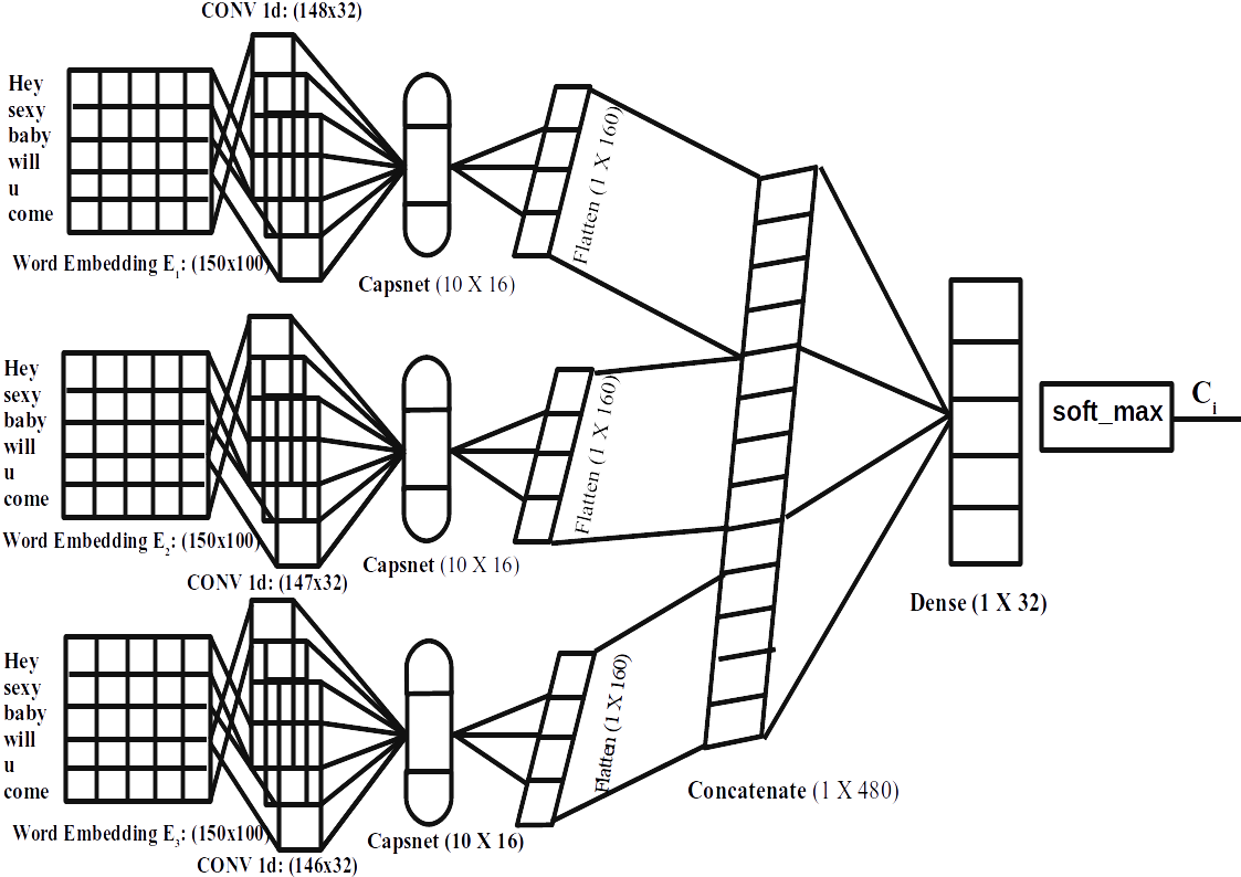
Figure 1: Architecture of CN1 model

The tweets are first converted to lower case. Next, we remove digits, special characters, emojis, urls, and stop words. We restrict the continuous repetition of the same character in a word to 2 (e.g. ’suuuuuuper’ is converted to ’suuper’). Each tweet is tokenized and converted into a sequence of integers. The maximum sequence length is restricted to 150. To have dense representation of tokens, the following word embedding features are used:

• Glove++: Given the word, we first check whether it is present in Glove pre-trained 6b 100d embeddings, and use the embedding if it exists. For Out-Of-Vocabulary words, we use the word vectors that we train on the entire data using the Gensim library.

• Aggression Embeddings: To have distinguishing features to separate aggressive tweets from non-aggressive tweets, we create aggression word embeddings. We take all the tweets classified as OAG and CAG and train word vectors on them.

• Char Trigram: To get sub-word information, we create character trigram embeddings.

5 Proposed Architecture

We propose an architecture that combines features that are learned from an ensemble of subnetworks and leverages the feature representation to classify aggression. All models optimize the categorical crossentropy loss function using adam optimizer. All the dense layers, except the final layer, have ReLu activation. All the CNN layers are followed by dropout = 0.5. Every model is an ensemble of smaller subnetworks. Each subnetwork (SN) has the following configuration:

• Embedding layer - Each token in the input sequence is represented by its word vector. Word embeddings help to capture the meaning of the word.

• Convolutional layer - A convolutional layer, having reLu activation function, to extract spatial features.

• Max-pooling layer of size 2 or 3 in case of Deep Learning models.

• Capsule layer to better preserve spatial information, in case of Capsulenet models.

Each SN of the model uses a different configuration for the CNN layer or embedding. Therefore each SN learns different information and generates different features. The output of each SN is flattened and merged and is passed as input to dense layers. The last dense layer has three neurons and a softmax activation function, which gives a probability score to each of the three classes, and the one with the highest score is the predicted class.

5.1 Deep Learning (DL) Models

The following are the DL baselines:

DL1: It is an ensemble of three subnetworks. All three SNs use Glove++ embeddings for the embedding layer. The CNN layers in each SN have kernel sizes 3,5 and 7, respectively.
DL2: It is an ensemble of 9 SNs. Each max-pooling layer is followed by a biLSTM layer, having 200 units, to capture long term dependencies. SN 1-3 use Glove++ embeddings. SN 4-6 use Aggression embeddings. SN 7-9 use Character-level trigram embeddings. CNN layer in SN 1,4,7 has kernel size = 3, in SN 2,5,8 has kernel size = 5 and in SN 3,6,9 has kernel size = 7.

5.2 Capsule Network (CN) Models

The main difference between CN models and DL models is that the CN models use a capsule layer instead of max-pooling layer. The capsule layer has 10 capsules of 16 dimension each. Max-pooling reduces computational complexity but leads to the loss of spatial information.

Capsules are a group of neurons that are represented as vectors. The orientation of the feature vector is preserved in capsules. They use a function called squashing for non-linearity. Dynamic Routing is used to route the feature vector of the lower-level capsule to the appropriate next level capsule Sabour et al. (2017). Dynamic Routing is based on a coupling coefficient that measures the similarity between vectors that predict the upper capsule and the lower capsule and learns which lower capsule should be directed to which upper capsule Kim et al. (2018). Through this process, capsule layers preserve spatial information, learn semantic representation, and ignore words that are insignificant.
CN1: The architecture is shown in figure 1. It is an ensemble of 3 subnetworks. Each SN uses Glove++ embeddings, and the CNN layers have kernel size = 3,4 and 5, respectively.
CN2: Like CN1, but there is an additional biLSTM layer, having 300 units, after the capsule layer.

6 Results and Discussion

DL models		CN models
DL1	57.17%	CN1	65.20%
DL2	60.34%	CN2	62.70%

Table 2: Weighted F1 scores of DL and CN models

From table 2, we see that the CN models perform better than DL models. Both the CN models are comparable to the models proposed by Srivastava et al. (2018). This validates the usefulness of capsule networks for aggression detection. CN1 gives the best results and is better than the best model proposed by Aroyehun and Gelbukh (2018). DL2 works better than DL1, as it captures more information. The performance drops from CN1 to CN2, despite CN2 having an additional biLSTM layer. This shows that a more complex model is not necessarily better, which is in agreement with the observations of Aroyehun and Gelbukh (2018). This could be due to over-fitting.

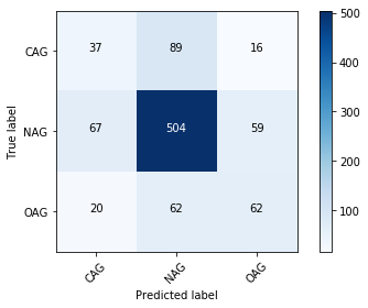
Figure 2: Confusion matrix of CN1 model

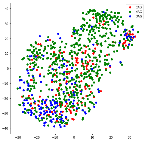
Figure 3: Flatten vector of subnetwork1

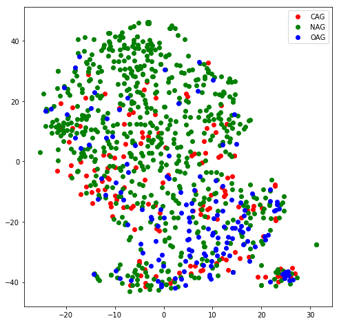
Figure 4: Flatten vector of subnetwork2

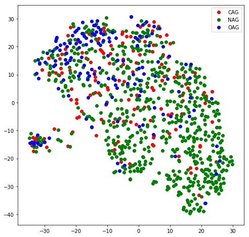
Figure 5: Flatten vector of subnetwork3

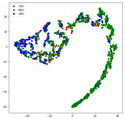
Figure 6: Performance of Output Layer

Figures 3, 4 and 5 are t-SNE van der Maaten and Hinton (2008) graphs, which depict the output of SN1-3 of CN1, respectively. We visualize the feature embeddings in all the SNs, and we observe that each SN is able to characterize the features distinctly due to the variability in the network configurations. When all the SNs are combined in an ensemble network, the feature representation is further improved. The inter-class variability is predominant, as can be validated in Fig. 6. This can be attributed to the fact that all 3 SNs have complimentary feature representations.

As observed from the confusion matrix of CN1 model ( Fig. 2), NAG is the easiest to detect. It is because most of the tweets in the data are NAG. The performance is better on OAG than on CAG, despite there being more training examples of CAG as OAG is more explicit and hence easier to identify, as opposed to the more indirect CAG Davidson et al. (2017). CAG, because of its covert nature is the most difficult to classify. The confusion of CAG can also be observed in figure 6, where CAG is overlapping with NAG and OAG.

The confusion can also be seen by analyzing some CAG tweets predicted as NAG:
”Hundreds of people were killed by your friends in Bombay, where were you at that time.”
”What’s next? Soon we will be told to have a bullock cart and give up cars? Or live in a shed using candles?”
”Chit fund operators n loan sharks r more honest”

7 Conclusion and Future Work

We perform experiments to identify aggressive tweets by applying DL and Capsule Networks on preprocessed data. We show that capsulenets are efficient for aggression detection. We use an ensemble-based model and qualitatively show that each subnetwork learns unique features which help in classification. Our best model uses capsulenets and results in a 65.20% f1 score, which is an improvement over most of the existing solutions.

In the future, we would like to explore other capsulenet architectures using different routing algorithms. A more in-depth analysis of CAG tweets could improve the performance on them.

8 Acknowledgement

We thank the anonymous reviewers for their constructive feedback. We also thank Rohan Sukumaran and Harshit Singh for fruitful discussions and proofreading.

References

- Aroyehun and Gelbukh (2018) Segun Taofeek Aroyehun and Alexander Gelbukh. 2018. Aggression detection in social media: Using deep neural networks, data augmentation, and pseudo labeling. In TRAC - 2018, pages 90–97.
- Badjatiya et al. (2017) Pinkesh Badjatiya, Shashank Gupta, Manish Gupta, and Vasudeva Varma. 2017. Deep learning for hate speech detection in tweets. In Proceedings of the 26th International Conference on World Wide Web Companion, WWW ’17 Companion, pages 759–760, Republic and Canton of Geneva, Switzerland. International World Wide Web Conferences Steering Committee.
- Bhattacharja (2010) Shishir Bhattacharja. 2010. Bengali verbs: a case of code-mixing in Bengali. In Proceedings of the 24th Pacific Asia Conference on Language, Information and Computation, pages 75–84, Sendai, Japan.
- Dadvar et al. (2013) Maral Dadvar, Dolf Trieschnigg, Roeland Ordelman, and Franciska de Jong. 2013. Improving cyberbullying detection with user context. In Advances in Information Retrieval, pages 693–696.
- Davidson et al. (2017) Thomas Davidson, Dana Warmsley, Michael Macy, and Ingmar Weber. 2017. Automated hate speech detection and the problem of offensive language. ICWSM ’17, pages 512–515.
- Khandelwal and Kumar (2020) Anant Khandelwal and Niraj Kumar. 2020. A unified system for aggression identification in english code-mixed and uni-lingual texts. In Proceedings of the 7th ACM IKDD CoDS and 25th COMAD, CoDS COMAD 2020, page 55–64, New York, NY, USA. Association for Computing Machinery.
- Kim et al. (2018) Jaeyoung Kim, Sion Jang, Sungchul Choi, and Eunjeong L. Park. 2018. Text classification using capsules. CoRR, abs/1808.03976.
- Kumar et al. (2018a) Ritesh Kumar, Atul Kr. Ojha, Shervin Malmasi, and Marcos Zampieri. 2018a. Benchmarking aggression identification in social media. In TRAC-2018, pages 1–11.
- Kumar et al. (2020) Ritesh Kumar, Atul Kr. Ojha, Shervin Malmasi, and Marcos Zampieri. 2020. Evaluating aggression identification in social media. In Proceedings of the Second Workshop on Trolling, Aggression and Cyberbullying, pages 1–5, Marseille, France. European Language Resources Association (ELRA).
- Kumar et al. (2018b) Ritesh Kumar, Aishwarya N. Reganti, Akshit Bhatia, and Tushar Maheshwari. 2018b. Aggression-annotated corpus of hindi-english code-mixed data. CoRR, abs/1803.09402.
- Kumari and Singh (2020) Kirti Kumari and Jyoti Prakash Singh. 2020. AI_ML_NIT_Patna @ TRAC - 2: Deep learning approach for multi-lingual aggression identification. In Proceedings of the Second Workshop on Trolling, Aggression and Cyberbullying, pages 113–119, Marseille, France. European Language Resources Association (ELRA).
- van der Maaten and Hinton (2008) Laurens van der Maaten and Geoffrey Hinton. 2008. Visualizing data using t-SNE. Journal of Machine Learning Research, 9:2579–2605.
- Mikolov et al. (2013) Tomas Mikolov, Kai Chen, Greg Corrado, and Jeffrey Dean. 2013. Efficient estimation of word representations in vector space. CoRR, abs/1301.3781.
- Nobata et al. (2016) Chikashi Nobata, Joel Tetreault, Achint Thomas, Yashar Mehdad, and Yi Chang. 2016. Abusive language detection in online user content. In Proceedings of the 25th International Conference on World Wide Web, WWW ’16, pages 145–153, Republic and Canton of Geneva, Switzerland. International World Wide Web Conferences Steering Committee.
- O’Neal (1994) Edgar C. O’Neal. 1994. Human aggression, second edition, edited by robert a. baron and deborah r. richardson. new york, plenum, 1994, xx + 419 pp. Aggressive Behavior, 20(6):461–463.
- Risch and Krestel (2018) Julian Risch and Ralf Krestel. 2018. Aggression identification using deep learning and data augmentation. In TRAC-2018, pages 150–158.
- Risch and Krestel (2020) Julian Risch and Ralf Krestel. 2020. Bagging BERT models for robust aggression identification. In Proceedings of the Second Workshop on Trolling, Aggression and Cyberbullying, pages 55–61, Marseille, France. European Language Resources Association (ELRA).
- Roy et al. (2018) Arjun Roy, Prashant Kapil, Kingshuk Basak, and Asif Ekbal. 2018. An ensemble approach for aggression identification in english and hindi text. In TRAC-2018, pages 66–73.
- Sabour et al. (2017) Sara Sabour, Nicholas Frosst, and Geoffrey E Hinton. 2017. Dynamic Routing Between Capsules. arXiv e-prints, page arXiv:1710.09829.
- Safi Samghabadi et al. (2018) Niloofar Safi Samghabadi, Deepthi Mave, Sudipta Kar, and Thamar Solorio. 2018. RiTUAL-UH at TRAC 2018 shared task: Aggression identification. In Proceedings of the First Workshop on Trolling, Aggression and Cyberbullying (TRAC-2018), pages 12–18, Santa Fe, New Mexico, USA. Association for Computational Linguistics.
- Safi Samghabadi et al. (2020) Niloofar Safi Samghabadi, Parth Patwa, Srinivas PYKL, Prerana Mukherjee, Amitava Das, and Thamar Solorio. 2020. Aggression and misogyny detection using BERT: A multi-task approach. In Proceedings of the Second Workshop on Trolling, Aggression and Cyberbullying, pages 126–131, Marseille, France. European Language Resources Association (ELRA).
- Srivastava et al. (2018) Saurabh Srivastava, Prerna Khurana, and Vartika Tewari. 2018. Identifying aggression and toxicity in comments using capsule network. In TRAC-2018, pages 98–105.
- Wang et al. (2018) Yequan Wang, Aixin Sun, Jialong Han, Ying Liu, and Xiaoyan Zhu. 2018. Sentiment analysis by capsules. In Proceedings of the 2018 World Wide Web Conference, WWW ’18, pages 1165–1174, Republic and Canton of Geneva, Switzerland. International World Wide Web Conferences Steering Committee.
- Zhao et al. (2018) Wei Zhao, Jianbo Ye, Min Yang, Zeyang Lei, Suofei Zhang, and Zhou Zhao. 2018. Investigating capsule networks with dynamic routing for text classification. CoRR, abs/1804.00538.