A Low-Delay MAC for IoT Applications: Decentralized Optimal Scheduling of Queues without Explicit State Information Sharing

Abstract

We consider a system of several collocated nodes sharing a time slotted wireless channel, and seek a MAC (medium access control) that (i) provides low mean delay, (ii) has distributed control (i.e., there is no central scheduler), and (iii) does not require explicit exchange of state information or control signals. The design of such MAC protocols must keep in mind the need for contention access at light traffic, and scheduled access in heavy traffic, leading to the long-standing interest in hybrid, adaptive MACs.

Working in the discrete time setting, for the distributed MAC design, we consider a practical information structure where each node has local information and some common information obtained from overhearing. In this setting, “ZMAC” is an existing protocol that is hybrid and adaptive. We approach the problem via two steps (1) We show that it is sufficient for the policy to be “greedy” and “exhaustive.” Limiting the policy to this class reduces the problem to obtaining a queue switching policy at queue emptiness instants. (2) Formulating the delay optimal scheduling as a POMDP (partially observed Markov decision process), we show that the optimal switching rule is Stochastic Largest Queue (SLQ).

Using this theory as the basis, we then develop a practical distributed scheduler, QZMAC, which is also tunable. We implement QZMAC on standard off-the-shelf TelosB motes and also use simulations to compare QZMAC with the full-knowledge centralized scheduler, and with ZMAC. We use our implementation to study the impact of false detection while overhearing the common information, and the efficiency of QZMAC. Our simulation results show that the mean delay with QZMAC is close that of the full-knowledge centralized scheduler.

I Introduction

In the Internet of Things (IoT), wireless access networks will connect embedded sensors to the infrastructure network. Since these embedded devices will be resource challenged, the wireless medium access control (MAC) protocols will need to be simple, and decentralized, and not require explicit exchange of state information and control signals. However, some of the emerging applications over IoT networks might expect low packet delivery delays as well [2]. In this paper, we report our work on developing a low mean delay MAC protocol for $N$ collocated nodes sharing a time slotted wireless channel, such that there is no centralized control and no explicit exchange of state information. Networks with collocated nodes regularly arise in the industrial IoT setting, specifically, machine health monitoring [3]. Emerging standards for IoT applications, such as the DetNet and 6TiSCH [4], have shown considerable interest in systems with a synchronous time-slotted framework. It may be noted that, for this setting, a centralized scheduler with full queue length information can just schedule any nonempty queue in each slot. The challenge we address in this paper is to develop a distributed mechanism, without explicit exchange of queue length information, that achieves mean delay very close to that of the centralized scheduler.

It is well known that, while contention access (ALOHA, CSMA etc.) performs well at low contention, it can result in very large delays and possibly instability under high contention [5]. While attempts have been made to stabilize CSMA, the delay of these algorithms still remains prohibitively high [6, 7, 8]. Polled access (e.g., 1-limited cyclic service [9], which we will call TDMA in this paper) on the other hand, shows the opposite behavior. It is, hence, desirable to have protocols that can behave like TDMA under high contention and CSMA under low contention. The qualitative sketch in Fig. 1 illustrates this behavior. The figure compares the delay performance of polling and contention MACs (orange and blue, respectively) showing the phenomenon discussed above. Also shown are two illustrations of “load adaptive” performance expected of hybrid MACs, the one in red being uniformly better than the one in green. The figure also shows the lowest possible delay attainable in this setting (black curve). This curve is discussed in more detail in Sec. VII, where we show that the hybrid MACs proposed in this paper come extremely close to this curve and, hence, are nearly delay optimal.

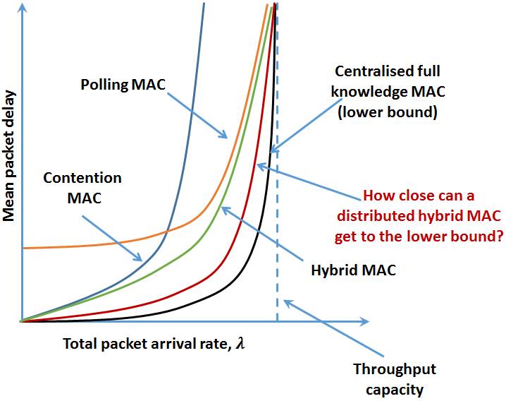
Figure 1: A sketch of the delay performance of various MAC protocols. Arrival rates to all queues are assumed equal. Throughput capacity = 1, i.e. $\lambda\in[0,1)$.

There have been many attempts at proposing protocols that achieve this, especially in the context of wireless sensor networks. Important examples include [10, 11, 12, 13, 14, 15, 16] and [17]. Among these, ZMAC [15] has been observed to perform the best in terms of delay and channel utilization (see [18]), and will be an important point of comparison in this paper. ZMAC’s delay performance, however, is quite poor compared to centralized scheduling with full queue length knowledge (see Fig. 7(b)). The question, therefore, remains whether we can achieve low delay, in a decentralized setting, in which the information available to each node is just what it can acquire by “listening” over the channel.
Moreover, the design of the aforementioned protocols has been heuristic and without theoretical explanation of optimal scheduling of queues. Further, little attention appears to have been paid to distributed scheduling in the TDMA context, such that each node uses only locally available information. If all queue lengths are known at a central scheduler, then ideal performance can be achieved. In the context of partial information about queue occupancies, the aim, at each scheduling instant, is to minimize the time it takes for the system to find a nonempty queue and allow it to transmit. How this can be achieved in the setting of collocated nodes with a common receiver, by using stochastic optimal control (with partial information) in conjunction with extensions of known results on optimal scheduling, is the main contribution of this paper.

I-A Our Contributions

We consider $N$ nodes sharing a slotted wireless channel to transmit packets (each of which fits into one slot) to a common receiver. Each node receives a stochastic arrival process embedded at the slot boundaries. We begin by describing in detail the structure of the (partial) information that nodes in the network will be assumed to possess, in Sec. II. This structure will inform the development of optimal scheduling policies and distributed scheduling protocols.

• We then prove the delay optimality of greedy and exhaustive service policies in this novel partial information setting (in Sec. III-C). While our analysis employs proof techniques in [19] to show sample pathwise dominance, the added complexity of state dependent server switchover delays complicates the analysis in this (and the next) section considerably.

• Focusing on greedy and exhaustive service policies, with no explicit queue length information being shared between nodes, we derive a mean delay optimal policy by formulating the problem as a Markov decision process with partial information (Sec. III-D). We initially cast the problem as an $\alpha$-discounted cost MDP, obtain the optimal policy, and extend the result to time-average costs (Sec. III-D4). We also use Foster Lyapunov theory [20] to modify and extend our proposed optimal policy to solve the problem of unfairness that it gives rise to in our Technical Report [21, Sec. 4.6]. Further, we discuss how our results can also handle channel errors and fading.

• We then use our delay optimality results to design two Hybrid MAC protocols (EZMAC and QZMAC) and show that the delays achieved by them are much lower than that achieved by ZMAC (Sec. V). We then present modifications to QZMAC to handle unequal arrival rates, alarm traffic and Clear Channel Assessment (CCA) errors. To the best of our knowledge, this is the first work that deals with hybrid MAC scheduling for systems with unequal arrival rates (Prop. 3 and Thm. 5).

• We report the results of implementing QZMAC over a collocated network comprising CC2420 based Crossbow telosB motes running the 6TiSCH [2] communication stack, in Sec. IX-A. In Sec. VII, we present simulation results comparing the delay (both mean and delay CDF) performance of QZMAC and EZMAC with that of ZMAC. We also show that delay with QZMAC is very close to the minimum delay that can be obtained in this scenario (Sec. VII-B). We discuss techniques to tune QZMAC to modify its performance over different portions of the network capacity region (see Eqn.(2)) and also compare the Channel Utilization of QZMAC with that of ZMAC. Finally, we conclude the paper and present directions for future research.

II Frame Structure and System Processes

We consider a wireless network comprising several source nodes (e.g., sensor nodes) transmitting to a common receiver node (e.g., a base station). The nodes are collocated in the sense that all nodes can hear each other’s transmissions. This could mean, at one extreme, that they can decode each other’s transmissions, or just sense each other’s transmissions. We will comment on this further in Sec. IV. Time is assumed slotted; the slots are indexed $t=0,1,2,\cdots$, with slot $t$ being bounded by the epochs $t$ and $t+1$. In each slot $t$, a single node can transmit successfully (note that there is a common receiver). If a node transmits in slot $t$, at the end of the slot, i.e., at instant $t+1$, that node is viewed as the “node under service,” or the “incumbent,” the identity of which is assumed known to all the nodes, a property that is ensured by the information structure and our distributed algorithms.

We model the system as a network of $N$ parallel queues with a single shared server, whose service has to be scheduled between the $N$ queues. We denote by $A_{j}(t)$, the number of arrivals to Queue $j$ at time slot boundary $t~{}(t=0,1,2,\cdots)$. $A_{j}(t)$ is assumed i.i.d Bernoulli with $P\{A_{j}(t)=1\}=\lambda_{j}$. The arrival processes are assumed independent of each other and the system backlog. The backlog at Queue $j$ at the beginning of time slot $t$ (i.e., at $t+$) is denoted by $Q_{j}(t)$ (see Fig. 2). We assume that each slot can carry exactly one data packet, after allowing time for any protocol overhead. A packet transmission from Node $j$ in slot $t$ leads to a “departure” from the corresponding queue, which is viewed as occurring at $(t+1)-$, i.e., just before the end of slot $t$. $D_{j}(t)\in\{0,1\}$ indicates whether Queue $j$ is scheduled for service in slot $t.$ We assume packet transmission success probability to be $1$ and remove this assumption in [21, Sec. 11.12]. It follows from the embedding of the processes described, that the evolution of the queue-length process at Queue $j$ can be described by.

$$Q_{j}(t+1) = (Q_{j}(t)-D_{j}(t))^{+}+A_{j}(t+1),$$ (1)

$$Q_{j}(0) = A_{j}(0),$$

where for all $x\in\mathbb{R},(x)^{+}=$max$(x,0)$.
Stability and Delay. Since at most one queue (equivalently, “node”) can be scheduled for transmission in a slot and at most one packet can be transmitted in one slot, the capacity region [22] of this system is given by

$$\boldsymbol{\Lambda}=\left\{\boldsymbol{\lambda}\in\mathbb{R}^{N}_{+}:\sum_{j=1}^{N}\lambda_{j}<1\right\}.$$ (2)

Define $\mathbf{Q}(t)=\left[Q_{1}(t),\cdots,Q_{N}(t)\right],~{}t\geq 0.$ We say that the system is stable if the system backlog Markov chain, $\left\{\mathbf{Q}(t),~{}t\geq 0\right\}$, is positive recurrent. A protocol that is capable of stabilizing any vector in $\mathbf{\Lambda}$ is said to be Throughput Optimal [22]. Delay is defined as the number of slots between the instant a packet enters a queue and the instant it leaves the queue. Note that this along with the embedding described so far means that a packet experiences a delay of at least one slot.

Figure 2: Figure showing how the queue length, arrival and service processes are embedded.

Let $Q_{j}\stackrel{{\scriptstyle\Delta}}{{=}}\lim_{t\rightarrow\infty}\frac{1}{t}\sum_{\tau=0}^{t-1}Q_{j}(\tau)$, let $W_{j}(k)$ denote the delay experienced by the $k^{th}$ packet in Queue $j$ and $W_{j}\stackrel{{\scriptstyle\Delta}}{{=}}\lim_{L\rightarrow\infty}\frac{1}{L}\sum_{k=0}^{L-1}W_{j}(k)$. Under stability, $Q_{j}$ and $W_{j}$ are constant with probability one; we denote these constants also by $Q_{j}$ and $W_{j}$. Using Little’s Theorem, $W_{j}=\frac{Q_{j}}{\lambda_{j}}$. The delay experienced by a packet randomly chosen from the arriving stream, therefore, is given by $W=\sum_{j=1}^{N}\left(\frac{\lambda_{j}}{\sum_{k=1}^{N}\lambda_{k}}\right)W_{j}=\frac{1}{{\sum_{k=1}^{N}\lambda_{k}}}\sum_{j=1}^{N}Q_{j}$. Our objective in the paper is to develop decentralized protocols that minimize $W.$
Centralized vs Distributed Scheduling. In the setting described in Sec. II, if, at the beginning of every slot, the queue lengths are all known to a central scheduler, then (assuming zero queue-switching overheads) it suffices to simply schedule any nonempty queue. The sum queue length process would then be stochastically equivalent to a discrete time, work conserving, single server queue, whose arrival process is the superposition of the $N$ arrival processes. The mean delay (equivalently, the mean queue length) would then be the smallest possible. We, however, wish to avoid any explicit dissemination of queue length information over the network, and aim to develop a scheduler that the nodes implement in a decentralized fashion.

III Delay Optimal Multiqueue Scheduling with Local and Common Queue Length Information

Information Structure. Assuming that the collocated setting is such that all nodes can overhear and decode each other’s transmissions, we consider the following natural information structure for the multiqueue scheduling problem. If each transmitted packet carries the queue length of the node at the instant it is transmitted, at the beginning of each slot, every node knows the length of every queue at the beginning of every slot in which the queue was allowed to transmit. At the beginning of slot $t$, each queue knows $\left\{Q^{\pi}_{j}\left(\left(t-V_{j}^{\pi}(t)\right)-\right),~{}j\in I\right\}$, where $V_{j}^{\pi}(t)$ is the number of slots prior to slot $t$ in which Queue $j$ was allowed to transmit under a generic scheduling policy $\pi$ (the term “policy” is formally defined in Sec. III-B below). As an example, if the incumbent is Queue $k$, the packet transmitted in Slot $t-1$ would have carried the queue length $Q^{\pi}_{k}(t-1)$; since one packet was transmitted, $Q^{\pi}_{k}(t-)=Q^{\pi}_{k}(t)-1$, and, since $V^{\pi}_{k}(t)=0$, this is also $Q^{\pi}_{k}\left(\left(t-V^{\pi}_{k}(t)\right)-\right)$.

In the literature, $V_{j}^{\pi}(t)$ is also called “Time Since Last Service” (TSLS) [23]. In addition, at the beginning of slot $t$, every node evidently knows its own queue length; this can be viewed as local information at Queue $j$. We seek a distributed scheduling policy where each node acts autonomously based on the queue information structure above, while aiming to achieve a global performance objective (say, minimizing the time average total queue length in the system).

III-A Our approach to developing an optimal policy

Our approach is via two optimal scheduling problems that each requires more than the common information.
The first problem, formulated in Sec. III-B, uses the common information (outlined above) and the incumbent’s queue length (which is actually known only to the incumbent), to establish that, for every scheduling policy, there is a greedy and exhaustive scheduler that yields stochastically smaller queue lengths (Sec. III-C). Due to this result, we can limit ourselves to greedy and exhaustive schedulers.
Once we limit to a greedy and exhaustive scheduler, effectively, the decision instants are those at which the incumbent queue becomes empty, at which instants a decision has to be made to switch to one of the other queues. We formulate this second problem via an average cost Markov decision process (Sec. III-D1), for which the available information is the common information and some additional information. We show that, for equal arrival rates ($\lambda_{k}=\lambda,k\in I$), an optimal policy is Stochastic Longest Queue, i.e., at an instant at which an incumbent becomes empty, the queue to which the service switches must not be smaller than any other queue in the stochastic ordering sense. This is also equivalent to serving the Longest Expected Queue (LEQ), albeit with equal arrival rates. Finally, the implementation of this policy only requires a distributed means for all nodes to realize that the incumbent has become empty. In Sec. IV, we use a technique from [15] for providing this additional information to all the nodes, thus implementing the distributed scheduler, which works only with a single bit of common information known to all the nodes, by virtue of overhearing.

III-B Problem 1: Centralized Scheduling with an Augmented Information Structure

A centralized scheduler is defined by a scheduling policy say $\pi$, which (informally speaking), at the beginning of slot $t$, i.e., at $t+$, uses the available information and past actions to determine which queue (if any) should be allowed to transmit in slot $t$. We indicate the use of a given policy $\pi$ by placing the superscript $\pi$ on all processes associated with the system; for example, $Q^{\pi}_{j}(t),~{}t\in\{0,1,\cdots\}$ is the queue length process of Node $j$ under the policy $\pi$. At the beginning of slot $t,~{}t\geq 1$, we denote by $\pi^{q}_{t-1}$, the queue that had been scheduled in the previous slot, or, equivalently the “incumbent” at the beginning of slot $t.$
Notation for policies. Under policy $\pi$, the action at $t+$ is denoted by $\mathcal{A}^{\pi}_{t}:=(\pi^{a}_{t},\pi^{q}_{t}),$ where $\pi^{a}_{t}$ represents the action to be taken during slot $t$ and $\pi^{q}_{t},$ the queue upon which the action is to be performed. $\pi^{a}_{t}\in\{0,1,s_{0},s_{1}\}$ which mean respectively, idle at $\pi^{q}_{t}=\pi^{q}_{t-1}$, serve $\pi^{q}_{t}=\pi^{q}_{t-1}$ if nonempty, switch (away from queue $\pi^{q}_{t-1}$) to $\pi^{q}_{t}$ and idle there, and switch to $\pi^{q}_{t}$ and serve it if nonempty. With the above in mind, and anticipating a result similar to [19, Prop. 3.2], we consider a centralized scheduler that has the following information. For every $t\geq 1$ and policy $\pi$, the “history” of the policy contains (i) all the actions taken until $t-1,$ (ii) the backlog of each queue at the last instant it was allowed to transmit, (iii) the instants at which this backlog was revealed, and (iv) the backlog of the incumbent at $t$, i.e.,

$$H^{\pi}_{t} := \left\{\left(\mathcal{A}^{\pi}_{m}\right)_{m=0}^{t-1};\left(Q^{\pi}_{j}\left(\left(t-V_{j}^{\pi}(t)\right)-\right)\right)_{j=1}^{N};\right.$$ (3)

$$\left.\left(V_{j}^{\pi}(t)\right)_{j=1}^{N};Q^{\pi}_{\pi^{q}_{t-1}}(t)\right\}.$$

With reference to the information structure defined at the beginning of Sec. III, the common information available to all nodes at $t$ is in $H^{\pi}_{t}$. Let $\mathbb{H}^{\pi}_{t}$ denote the set of all histories under $\pi$ up to time $t$. A deterministic admissible policy is defined as a sequence of measurable functions from $\mathbb{H}^{\pi}_{t}$ into the action space $\mathbb{A}=\left\{0,1,s_{0},s_{1}\right\}\times I$. For policy $\pi$, define

$$Q^{\pi}(t)=\sum_{i=1}^{N}Q^{\pi}_{i}(t),$$ (4)

as the total backlog in the system at the beginning of time slot $t,~{}\forall t\geq 0$. Let the space of all admissible policies be denoted by $\Pi$. A policy $\pi\in\Pi$ is said to be

• greedy or non-idling if the server never idles at a nonempty queue, i.e., at $t,$ if the incumbent queue is nonempty, it must be served again, if the decision is not to switch away. The set of all such policies is denoted by $\Pi_{g}\subset\Pi,$ so
  $\Pi_{g}=\left\{\pi\in\Pi\mid Q_{\pi^{q}_{t-1}}(t)>0\Rightarrow\mathcal{A}^{\pi}_{t}\in\left\{1,s_{0},s_{1}\right\}\times I,~{}\forall t\geq 0\right\}$.

• exhaustive if the server never switches away from a nonempty queue. This set is denoted by $\Pi_{e}\subset\Pi$, i.e.,
  $\Pi_{e}=\left\{\pi\in\Pi\mid Q_{\pi^{q}_{t-1}}(t)>0\Rightarrow\mathcal{A}^{\pi}_{t}\in\left\{0,1\right\}\times\left\{\pi^{q}_{t-1}\right\},~{}\forall t\geq 0\right\}$.

We will now present several results with regards to scheduling in this system that will aid our design process.

III-C Optimality of Non-idling and Exhaustive Policies

On applying the next proposition to the centralized problem, we need only restrict attention to policies that let an incumbent continue to transmit its packets until a time $t$ at which its queue is empty. As long as the incumbent has packets, it is optimal not to idle (i.e., transmit in every slot).

Proposition 1.

For the system defined in Sec. III and for any policy $\pi\in\Pi$, $\exists~{}\xi\in\Pi_{g}\cap\Pi_{e}$, such that

$$Q^{\xi}(t)\stackrel{{\scriptstyle st}}{{\leq}}Q^{\pi}(t),~{}\forall~{}t\geq 0,$$ (5)

where “$st$” denotes stochastic ordering.

Proof:

The structure of the model is similar to the one in [19], and the result we seek is the same as [19, Prop. 4.2]. There, the model is a centrally scheduled system of queues, with i.i.d. service times, nonzero i.i.d. queue switchover times, and knowledge of $\left\{Q_{i}(t-V_{i,t}^{\pi}),~{}1\leq i\leq N\right\}$. Since switching times are nonzero, by exhaustively serving a queue the per packet switching time is reduced, rather than switching away from a nonempty queue and then switching back to it in order to complete the service of the remaining packets. However, a crucial assumption in [19] is that the scheduler instantaneously obtains the queue length of every queue to which it switches. This is important since this limits their study to schedulers that never waste time attempting to serve empty queues, since, upon finding a queue empty, the scheduler is assumed to immediately switch away to another queue.

In our system, all queues can observe the empty or nonempty status of a transmitter whenever it is allowed to transmit. However, while there are no explicit switching times, due to decentralized scheduling, at switching instants, time could be wasted by switching to empty queues, although other nonempty queues exist. In [21, Sec. 4.2], we extend the coupling argument in [19] to establish this result. ∎

Implication for a distributed scheduling policy. Prop. 1 leads to the following simplification for the distributed scheduling problem. Since it is optimal for an incumbent to serve its queue in a non-idling and exhaustive manner, a switching decision needs to be made only when the incumbent’s queue becomes empty. Thus, once an incumbent is chosen, we only need a distributed mechanism for all nodes to determine the time $t$ at which the incumbent’s queue becomes empty. At such a $t$, based on the common information $V^{\pi}_{j}(t),1\leq j\leq N$ (where, of course, the element corresponding to the just past incumbent would be 0) the next incumbent needs to be selected in a distributed manner. We answer this question in Sec. III-D and Prop. 3.

Remark.

We are now working with truly common information unlike (3) where $Q^{\pi}_{\pi^{q}_{t-1}}(t),$ was known only to the incumbent.

III-D Equal Arrival Rates: Mean Delay Optimality of SLQ

In this section we show that, when the arrival rates at all queues are equal, SLQ is mean delay optimal. The stability region with equal arrival rates is obviously the interval $\lambda=[0,1/N)$. When the incumbent queue becomes empty at some $t$, the next incumbent has to be chosen in a distributed way, and if the chosen queue turns out to be empty as well then a slot is wasted.

We call a policy $\pi\in\Pi$ an SLQ (stochastically largest queue) policy if, at every instant $t$, in which a switchover takes place, the new queue chosen is not stochastically smaller than any other queue in the system. Formally, this means that whenever $\pi_{t}^{q}\neq\pi_{t-1}^{q}$, $V_{\pi_{t}^{q}}(t)\geq V_{k}(t)$ for every $k\in I$. The name SLQ arises from the fact that if $V_{l}>V_{k}$, and the two queues were served exhaustively, their current queue lengths, with Bernoulli arrivals, are Binomial($V_{l},\lambda$) and Binomial($V_{k},\lambda$) random variables respectively. Under these conditions, we know that Binomial($V_{l},\lambda$) is stochastically larger than Binomial($V_{k},\lambda$). Hence, the name.

Remark.

Recall that all scheduling decisions are made at the beginnings of slots and the only information available then is whether the incumbent queue is empty and the number of slots since each queue in the system was last allowed to transmit . It is this slot-wastage, which happens if the chosen queue is empty, that prevents us from using Prop. 5.1 of [19] by simply reinterpreting such wasted slots as a part of switchover times.

We now explicitly derive the delay optimal policy for equal arrival rate into all the queues, by formulating the problem as a Markov decision process (MDP).

III-D1 Mean Delay Optimality of SLQ

Motivated by Prop. 5, we restrict ourselves to policies in which the channel is acquired by another queue only if the queue under service is empty at the beginning of a slot. Suppose the queue scheduled in slot $t$ is denoted by $\{u_{t},t\geq 0\}$. We seek a policy, say $\pi$, to choose $u_{0},u_{1},\cdots$ so as to minimize the long term average cost function

$$\limsup_{T\rightarrow\infty}\frac{1}{T}\mathbb{E}_{s(0)}\sum_{t=0}^{T-1}\left(\sum_{i=1}^{N}Q_{i}(t)\right),$$ (6)

where $s(0)=[Q_{1}(0),\cdots,Q_{N}(0)]$ is the initial state of the system. This is the mean long-term backlog in the system and, as described at the end of Sec. II can be used as a proxy for mean delay. We first cast the problem as an $\alpha$-discounted cost minimization problem which involves minimizing the total discounted cost

$$\mathbb{E}_{s(0)}\sum_{t=0}^{\infty}\alpha^{t}\left(\sum_{i=1}^{N}Q_{i}(t)\right),$$ (7)

where $\alpha\in(0,1)$ is the discount factor. We will later arrive at the solution to the long-term time averaged cost, (6), using a limiting procedure with a sequence of optimal policies $\pi_{k}$ corresponding to a sequence of discount factors $\alpha_{k}\uparrow 1$. In what follows, we invoke the results of Prop. 5, and focus only on $\Pi_{g}\cap\Pi_{e}$.

III-D2 Formulating The Discounted Cost MDP

We will consider an information structure that includes the common information, and some local information. At the beginning of slot $t$ all the queues know (i) the index of the incumbent (ii) the number of slots since every queue was last served $\{V_{k}(t),k\in I\}$ (iii) the queue-length of the incumbent (at $t$), and (iv) residual known queue lengths in the queues (if any). Although we begin with this elaborate information structure, which has common information (known at all nodes), and local information (known only to each node), it will turn out that the optimal policy is such that (a) the action it takes at $t$ is a function only of $\{V_{k}(t),k\in[N]\}$ and the empty-nonempty status of the incumbent, and (b) it serves queues exhaustively, so the residual known queue lengths in the queues are all zero. Thus, the information structure we have in our problem (plus, an item of information that easily shared with all the nodes by using a simple, known technique (Sec. IV)) is sufficient to implement the optimal policy we derive and the generalization of the information structure (above) is only required for the proof of delay optimality to go through.

The MDP, under the information structure wherein the queues know the backlog of the incumbent and $\mathbf{V}(t)$, has $s(t)=\left[Q_{u_{t-1}}(t);\mathbf{V}(t);\mathbf{r}(t);u_{t-1}\right]^{T}$ as its state. The new coordinate $\mathbf{r}(t)$ is explained as follows. At the beginning of slot $t$ (just after arrivals occur), the server knows that Queue $j$ ($j\neq u_{t-1}$) has length $r_{j}(t)+U_{j},$ where $U_{j}$ is a Binomial$(V_{j}(t),\lambda)$ random variable. To accommodate the new information $\mathbf{r}(t)$, we expand our focus to the class of policies that always serve any queue $j$ such that $r_{j}(t)>0$ in time slot $t$. This means that if some queue $j$ has $r_{j}(t)>0$ at the beginning of time slot $t$, it is served in that slot and not the incumbent ($u_{t-1}$), even if $Q_{u_{t-1}}(t)>0.$ The underlying principle is that we can serve any queue that is known to be nonempty at the beginning of the slot.

But these policies are still greedy and exhaustive, in the (restricted) sense that whenever $\mathbf{r}(t)=\mathbf{0}$ and $Q_{u_{t-1}}(t)>0$, $u_{t}=u_{t-1}$, i.e., if no other queue is known to have packets and the incumbent is nonempty, it is served. This is a purely technical construction required for the proof of Thm. 2 and, as we will show later, the optimal policy (i.e., cyclic exhaustive service) will not require the knowledge of $\mathbf{r}(t)$ at all. The action in every slot $t$ with an empty incumbent, involves choosing a queue $u_{t}\in I$ and the single-step cost is the expected sum of the current queue lengths conditioned on the current state, given by

$$c(s(t),u_{t})=\mathbb{E}\left[\sum_{i=1}^{N}Q_{i}(t)|s(t)\right]=Q_{u_{t-1}}(t)+\lambda\sum_{j\neq u_{t-1}}V_{j}(t)+\sum_{i\in I}r_{i}(t).$$ (8)

Define the state space as $\mathbb{S}:=\mathbb{N}\times\mathbb{N}^{N}\times\mathbb{N}^{N}\times I$ and optimal discounted cost $J^{*}:\mathbb{S}\longmapsto\mathbb{R}_{+}$ starting in state $s(0)\in\mathbb{S}$ as

$$J^{*}(s(0))=min_{\xi}~{}\mathbb{E}^{\xi}_{s(0)}\sum_{t=0}^{\infty}\alpha^{t}\mathbb{E}\left[\sum_{i=1}^{N}Q_{i}(t)|s(t)\right],$$ (9)

and let $q$ represent the backlog of Queue $i$, the incumbent. The Bellman Optimality equations [24] associated with the MDP formulation as described above are as given in (10) (we denote $J^{*}(q;\mathbf{V};\mathbf{r};i)$ by $J_{i}^{*}(q;\mathbf{V};\mathbf{r})$).

$$J^{*}_{i}(q>0;\mathbf{V};\mathbf{r}=\mathbf{0}) =q+\lambda\sum_{k\neq i}V_{k}+\alpha\mathbb{E}J^{*}_{i}\bigg{(}q-1+A;$$

$$V_{i}=0,\mathbf{V}_{-i}+\mathbf{1};\mathbf{r}=\mathbf{0}\bigg{)},$$

$$J^{*}_{i}(q=0;\mathbf{V};\mathbf{r}=\mathbf{0})=\lambda\sum_{k\neq i}V_{k}+\alpha\min_{j\neq i}\mathbb{E}J^{*}_{j}\bigg{(}B(V_{j});\hskip 56.9055pt$$

$$V_{j}=0,\mathbf{V}_{-j}+\mathbf{1};\mathbf{r}=\mathbf{0}\bigg{)},\hskip 56.9055pt$$ (10)

In (10), $A$ is a generic Bernoulli($\lambda$) random variable, $\mathbf{V}_{-i}=[V_{1},\cdots,V_{i-1},V_{i+1},\cdots,V_{N}]$ and $\mathbf{1}\in\mathbb{R}^{(N-1)}$ is the vector with 1’s at all coordinates. Finally, if random variable $C$ is distributed Binomial($V_{j},\lambda$), $B(V_{j})$ is a random variable whose distribution is the same as that of $(C-1)^{+}+A$. The detailed formulation of the MDP and the Bellman Optimality equations for the case where $r_{j}\geq 1$ for some $j\in I-\{i\}$ can be found in [21, Sec. 11.6].

III-D3 Solution to the Discounted Cost MDP

Clearly, no decision needs to be taken when either $q>0$ or (from Prop. 1,) when $\mathbf{r}\neq\mathbf{0}$. Since the policies we seek are non-idling and exhaustive, they will simply continue to serve the incumbent when $q>0$ and therefore, states with $\mathbf{r}\neq\mathbf{0}$ never actually arise. We will now show that if $q=0$ and $\mathbf{r}=\mathbf{0}$, the system must choose $n:=\arg\max_{j}V_{j}$. In what follows, let $V_{m}<V_{n}$ for some $m\in I,~{}\text{and}~{}n\neq m$. We now prove that choosing $n$ results in the least cost.

Theorem 2.

When $V_{m}<V_{n}$ and $\lambda_{i}=\lambda,~{}\forall i\in[N],$

$$\mathbb{E}J^{*}_{n}\bigg{(}B(V_{n});V^{\prime}_{n}=0,\mathbf{V}_{-n}+\mathbf{1};\mathbf{r}_{-n}=\mathbf{0}\bigg{)}\leq\hskip 28.45274pt$$

$$\mathbb{E}J^{*}_{m}\bigg{(}B(V_{m});V^{\prime}_{m}=0,\mathbf{V}_{-m}+\mathbf{1};\mathbf{r}_{-m}=\mathbf{0}\bigg{)}.$$ (11)

Proof.

The expectation in (11) is with respect to arrivals. Intuitively, with equal arrival rates, the queue that has not received service the longest is also the most likely to be non-empty. Hence, attempting to serve this queue will result in the slot being wasted with the least probability. The proof of the theorem can be found in [21, Sec. 11.7]. ∎

Implication for a Distributed Scheduler. The policy above, denoted $\pi^{*}$ in what follows, chooses $\arg\max_{j}V_{j}(t)$ in every slot $t$ with an empty incumbent; in addition, by exhaustive service $\mathbf{r}(t)=\mathbf{0}$ for all $t$. In other words, $\pi^{*}$ is a stationary Markov policy that, at the beginning of each slot, chooses the incumbent, if nonempty, and the queue that has not been served the longest until that epoch, if the incumbent is found empty.
Now, before moving on to our original average cost problem, we make an important observation about the LEQ scheduling policy. Recall that the LEQ policy chooses $arg~{}max_{1\leq i\leq N}\lambda_{i}V_{i}(t)$ at every decision instant.

Proposition 3.

The LEQ policy stabilizes all arrival rate vectors in the set

$$\Lambda_{LEQ}:=\bigg{\{}\boldsymbol{\lambda}\in\mathbb{R}^{N}_{+}\bigg{|}\sum_{i=1}^{N}\lambda_{i}<1~{}\text{and}~{}\min_{1\leq i\leq N}\lambda_{i}>0\bigg{\}}.$$ (12)

Proof:

The proof essentially involves showing that the expected time to find the next nonempty queue (after serving some queue exhaustively) is bounded. Refer to [21, Sec. 11.3] for details of the proof.∎

Remark.

With $\lambda_{i}=\lambda,\forall i$, we have and the policy is easily seen to be a cyclic exhaustive policy, i.e., queues are served in a fixed cycle, with each queue being served to exhaustion (for a quick example, see [21, Sec. 11.4]). $arg~{}max_{1\leq i\leq N}\lambda_{i}V_{i}(t)=arg~{}max_{1\leq i\leq N}V_{i}(t)$ and the policy reduces to a cyclic exhaustive service policy.

In the literature, $V_{j}(t)$ is also called Time-Since-Last-Service (TSLS). The TSLS-based algorithm proposed in [23] schedules queues in a round robin fashion and requires knowledge of the empty-non empty status of every queue in the network in every time slot. However our theoretical results and the QZMAC algorithm, both of which preceded [23], require this information of queues only at the last time they were served. Our algorithms, therefore, actually are amenable to decentralized implementation.
In Prop. LABEL:prop:classTOStatMarkovPolicies in the Appendix, we show that the class of stabilizing, stationary Markov policies is not a singleton, and the policies therein have different mean delays. Thus, $\pi^{*}$ is not a trivial solution to our MDP.

III-D4 The Average-Cost Criterion

We use the technique described in [25] to show that $\pi^{*}$ is optimal for the long term time-averaged cost criterion as well. We consider a sequence of discount factors $\{\alpha_{n}\}\uparrow 1$ and the corresponding optimal policies and show that under certain conditions, the limit point of this sequence solves the Average-Cost problem, i.e., (6). For details, refer [21, Sec. 4.5]. Furthermore, in [21, Thm. 3], we show another desirable property of $\pi^{*}$, namely, that it is throughput optimal.

III-E The Distributed SLQ Policy

From Prop. 1 we concluded that we can limit our scope to greedy and exhaustive policies. This left us with the problem of determining a switching rule when the scheduled queue is exhausted. From the MDP in Sec. III-D, for the case of equal arrival rates, we have just learnt that at such a switching point, say, $t$, assuming that all nodes know the number of slots back that each node was last served (i.e., $V_{k}(t),k\in[N]$), it is optimal to switch to a queue $arg~{}max_{k\in[N]}V_{k}(t)$. For equal arrival rates, this is the same as the SLQ or the LEQ policy.

The following issues remain in the design of a distributed policy. (1) The design of a distributed mechanism by which all nodes can determine that an incumbent node has an empty queue at a scheduling instant $t$ (Sec. IV). (2) Greedy and exhaustive service locks out all the other queues for a long time. This leads to short-term unfairness. At the end of Sec. VI-B, we introduce a technique to address this concern.

IV Mechanisms for Decentralized Scheduling

In this section, we describe mechanisms by which transmission and lack of transmission in a slot, by the incumbent node can be inferred by all other nodes in the system, without any explicit exchange of information. The lack of transmission by the incumbent node is the trigger for switching to another incumbent.
Transmission sensing: We assume that all nodes transmit at the same fixed power, and the maximum internode distance is such that every other node can sense the power from a transmitting node. Suppose a node has been scheduled to transmit in a slot. Then, whether or not the node actually transmits can be determined by the other nodes by averaging the received power over a small interval, akin to the CCA mechanism (Clear Channel Assessment) [26]. For reliable assessment, the slot will need to be of a certain length, and the distance between the nodes will need to be limited. Let such an activity sensing slot be called a minislot (Fig. 3). See Sec. IX-B for further details.

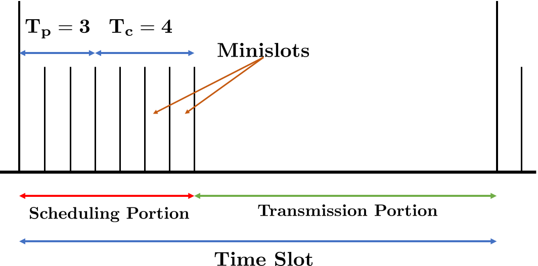
Figure 3: Illustrating the slot and minislot structures. Since $T_{p}=3$, three poll-and-test procedures can be performed by the system (incumbent plus two other queues). If none of these results in identifying a nonempty queue, the system goes into contention over the next $T_{c}=4$ minislots.

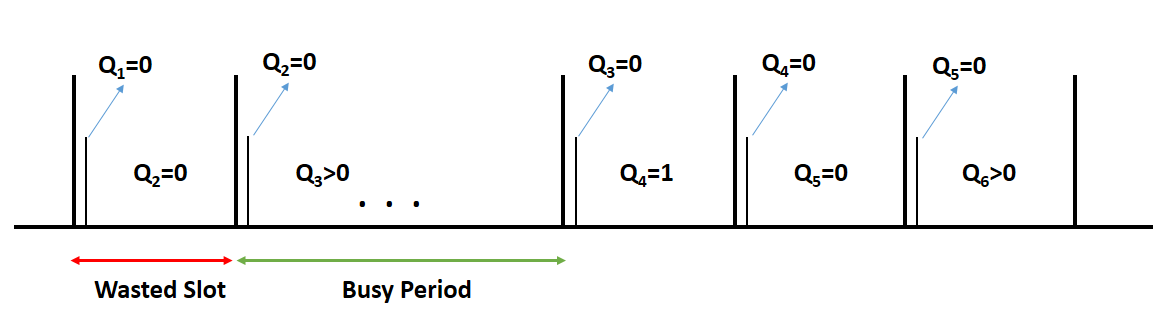
Figure 4: Sample path illustrating how $\pi^{*}$ is implemented in a system with $T_{p}=1$ and $T_{c}=0.$ Of particular note is the initially wasted slot. Since the poll-and-test did not identify any nonempty queue and since the system cannot go into contention ($T_{c}=0$), the slot is wasted.

Further optimization. (1) When an incumbent queue becomes empty (at, say $t$), an application of the policy results in switching to another queue (say, $k$). There is now a positive probability that $Q_{k}(t)=0$, which will result in the slot $t$ being wasted. The above approach of determining the emptying out of the incumbent’s queue can be used immediately in the same slot, if there is a provision of a second sensing slot. In this manner, if there are $T_{p}$ sensing slots, up to $T_{p}$ successive, wasteful switchings can be avoided. Each of these sensing actions can be viewed as a “poll-and-test” operation.
(2) In a light traffic setting, all the poll-and-test procedures might fail, with high probability. Having a large value of $T_{p}$ reduces this probability but increases the overhead. So, the next mechanism is contention, for which we have $T_{c}(\geq 0)$ minislots following the poll-and-test slots. The nodes that have not been polled can contend over these $T_{c}$ minislots, hopefully leading to the identification of one nonempty queue.
(3) Fig. 4 illustrates this mechanism for a simple system with $T_{p}=1,T_{c}=0$. In the first slot in the figure, the absence of power indicates, to all nodes in the network, that Node 1 is now empty and Node 2 is allowed to transmit. Since Node 2 is also empty, and since no more poll-and-test procedures are possible (since $T_{p}=1$), the slot is wasted. If $T_{p}=2$, and $T_{c}\geq 1$, sensing that Node 2 is empty, the other nonempty nodes in the network will contend for the slot.

V Protocol Design

In this section, use the results in Sec. III to motivate the practical design of our protocol, QZMAC. We will clearly describe how the optimal polling schemes in Section III-C are implemented in a distributed manner which will establish the self-organizing nature of our protocols.

V-A The EZMAC Protocol

We begin by explaining the limitations of ZMAC. As mentioned before, ZMAC first sets up a TDMA schedule allotting a slot to every queue in a cyclically-repeating frame, so $N$ nodes in the system means a frame with $N$ slots. Slot $j,~{}1\leq j\leq N,$ in every frame is assigned to Node $j$ which is called the Primary User (PU) in this slot. The other $(N-1)$ nodes, i.e., nodes $1,2,\cdots,j-1,j+1,\cdots,N,$ are called Secondary Users (SUs) in this slot. These SUs are allowed to contend for transmission rights in every TDMA slot with an empty PU. This is accomplished as follows. At the beginning of each time slot, each queue checks if it has a packet. If it does, and this is its TDMA slot (which means it is the PU), it proceeds to transmit the packet. If the current slot is NOT its TDMA slot, the queue first checks if the PU is transmitting (for a period of 1 minislot). If it hears nothing, it backs off over a duration chosen uniformly randomly over $\{T_{p}+1,\cdots,T_{p}+T_{c}\}$, and if the channel is clear, starts transmitting. Collisions are assumed to be detected instantaneously and that slot is assumed wasted. Note that a mechanism is needed to set up the TDMA schedule before transmissions can begin (e.g., DRAND [27]). The pseudocode for ZMAC is in our Tech Report [21, Sec. 6.1].

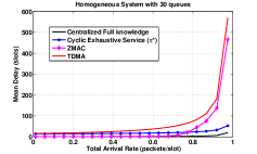
Figure 5: Comparing $\pi^{*}$ and ZMAC in a symmetric system with 30 queues. The total arrival rate to the system = $N\lambda\in[0,1)$.

As opposed to ZMAC, $\pi^{*}$ shows larger mean delay at lower arrival rates because the scheduled queue is, with high probability, going to be empty. It is for this reason that the mean delay curves of ZMAC and $\pi^{*}$ crossover near $\lambda=0.75$ in Fig. 5. In Sec. V-B, we solve this problem as well, and in doing so, arrive at the design of our protocol, QZMAC.

Our first protocol, EZMAC, differs from ZMAC in the contention resolution (CR) portion. Here, once the winner of a contention is determined, it is allowed to transmit in all slots without a PU until it empties. It is assumed that at the end of the winner’s transmission, the packet contains an end of transmission message (a bit in the header, perhaps) that can be decoded by the other users. We relegate details to [21, Sec. 6], but simulations results clearly show the improvement this change brings, to both mean delay and the delay CDF.

V-B The QZMAC protocol

In Sec. III-D2 we proved that cyclic exhaustive service is delay optimal in systems with equal arrival rates. Recall that Thm. 2 therein, assumed $T_{p}=1.$ However, we use this result to propose a scheduling protocol, QZMAC, for general $T_{p}\geq 1,$ and show through simulations that violating the $T_{p}=1$ assumption does not hurt the performance of QZMAC. Solving the MDP for general $T_{p}$ turns out to be a hard problem, and as simulation results in Figures 7(a) and 7(b) show, cannot result in any dramatic improvement in delay. We now describe QZMAC for $T_{p}=3$ minislots. Every queue maintains its own copy of a vector $\mathbf{V}(t)$ that is used to render the scheduling process fully distributed. The protocol proceeds as in Protocol. 1.

Protocol 1 QZMAC (with $T_{p}=3$ minislots),

1:Input: $N,T_{c}$$\triangleright$ This runs at every Queue $j,~{}j\in[N]$ in the network

2:Init: $t\leftarrow 0,\tau\leftarrow 1,PU\leftarrow 1,SU\leftarrow 2$ $\triangleright$ $\tau$ keeps track of the minislot number

3:Init: $\forall~{}k\in[N],V_{k}(0)\leftarrow k$

4:while $t\geq 0$ do $\tau\leftarrow 1$ $\triangleright$ Keeps track of minislot number.

5:    if $PU==j$ && $Q_{j}(t)>0$ then$\triangleright$ If you are the PU

6:         $PU$ transmits packet.

7:         for $k=1:N$ do

8:             $V_{k}(t)\leftarrow\left(V_{k}(t)+1\right)\mathbb{I}_{\{k\neq PU\}}$

9:         end for

10:         GOTO 35

11:    else

12:         $\tau\leftarrow\tau+1$ $\triangleright$ The 2^nd of $T_{p}$ minislots

13:         $i^{*}\leftarrow arg~{}max_{i\in[N]}V_{i}(t)$

14:         $PU\leftarrow i^{*}$

15:         if $i^{*}==j$ && $Q_{i^{*}}(t)>0$ then

16:             $PU$ transmits packet.

17:             for $k=1:N$ do

18:                 $V_{k}(t)\leftarrow\left(V_{k}(t)+1\right)\mathbb{I}_{\{k\neq PU\}}$

19:             end for

20:             GOTO 35

21:         else if $SU==j$ && $Q_{SU}(t)>0$ then

22:             $\tau\leftarrow\tau+1$ $\triangleright$ The last $T_{p}$ minislot

23:             $SU$ transmits packet.

24:             GOTO 35

25:         else$\triangleright$ SU empty $\Rightarrow$ network enters contention

26:             Over $\tau\in\{4,5,\cdots,T_{c}+3\}$ do

27:             if $Q_{j}(t)>0$ then $\triangleright$ Queue $j$ knows its own backlog

28:                 $U_{j}\sim Unif\left(\{4,5,\cdots,T_{c}+3\}\right)$

29:                 Wait for $U_{j}-4$ minislots.

30:                 If CCA == SUCCESS, Tx pkt.

31:                 If no collisions detected, $SU\leftarrow j$

32:             end if

33:         end if

34:    end if

35:     $t\leftarrow t+1$ $\triangleright$ Next time slot

36:end while

There are three points to note here. (1) QZMAC has clearly been obtained by separately optimizing polling and contention protocols. Jointly optimizing both turns out to be intractable and even separate optimization ultimately shows excellent delay performance. (2) Note that depending on the value of $T_{p}$, QZMAC can show a range of behavior. When $T_{p}=1$, the system never enters contention since one minislot is spent in ascertaining that the incumbent is empty and thereafter, $i^{*}$ (see Step 13) is allowed to transmit. Determining that $i^{*}$ is empty requires another minislot which is not available since $T_{p}=1$, and the system can enter contention only when $i^{*}$ and the SU are empty. So, in order for the system to enter contention, QZMAC needs $T_{p}=3$ (one each for the PU, $i^{*}$ and the SU). Similarly, ZMAC requires $T_{p}=1$. (3) As mentioned in Sec. III-D3, the use of the $\mathbf{V}(t)$ vector automatically induces a cyclic schedule. This is a much simpler technique than DRAND, used in ZMAC [27], which involves several rounds of communication among the nodes to converge to a TDMA schedule, even for fully connected interference graphs.

VI Extending QZMAC

In this section, we show how QZMAC can be modified to handle a variety of different applications.

VI-A Handling Unequal Arrival Rates

Prop. 3 helps generalize QZMAC very easily to accommodate unequal arrival rates. The only modification necessary here is to Step 13 where system now needs to choose $arg~{}max_{1\leq i\leq N}{\color[rgb]{0,0,1}\lambda_{i}}V_{i}(t)$. Clearly, finding $arg~{}max_{1\leq i\leq N}\lambda_{i}V_{i}(t)$ in every scheduling slot requires knowledge of the entire arrival rate vector $\boldsymbol{\lambda}$. Arrival rate estimation might not be feasible in several sensor networks of today that are expected to begin performing as soon as they are installed. For more information about this “peel and stick” paradigm refer to [2].

We resolve this problem by first observing that under stability, the time average of the total number of packets transmitted by any queue tends to the arrival rate. Let $D_{i}(t)$ be the random variable that denotes whether or not a departure occurred from queue $i$ at the end of slot $t$. Then, under stability, $\lim_{T\rightarrow\infty}(1/T)\sum_{t=0}^{T}D_{i}(t)=\lambda_{i},~{}a.s.$ So, let $\hat{\lambda}_{i}(T):=(1/T)\sum_{t=0}^{T}D_{i}(t).$ The policy that chooses $arg~{}max_{1\leq i\leq N}\hat{\lambda}_{i}(t)V_{i}(t)$ in every scheduling slot also shows the same mean delay performance as the LEQ policy, as evidenced by simulation results presented in Sec. VII-A. This estimate can be maintained independently at each queue and the resulting decisions are still consistent.

VI-B Handling CCA errors

We have, hitherto, assumed that when a network queue tests for channel activity (or lack thereof), the test always succeeds. In real wireless sensor networks this operation, called a Clear Channel Assessment (CCA), involves a hypothesis test based on noisy samples of channel activity and hence, is susceptible to error. This makes a 100% success rate a strong assumption and we relax it in this section. Notice that crucially, CCA errors affect the fidelity of the $\mathbf{V}(t)$ vector across nodes and we now have a matrix $V_{N\times N}(t)=[\mathbf{V}_{1}(t),\mathbf{V}_{2}(t),\cdots,\mathbf{V}_{N}(t)]$, where $\mathbf{V}_{i}(t)$ is the local copy at Queue $i.$

Extensive experimentation (reported in Sec. IX-A) reveals that absence of activity on the channel can be detected without error. This means that whenever a queue that is supposed to transmit (incumbent, $i^{*}=arg~{}max_{i\in[N]}V_{i}(t)$ or the SU) is empty, all CCAs across the network in that minislot report a “clear channel.” In detection theoretic parlance, the probability of a false alarm is zero, i.e., $p_{FA}=0$. On the other hand, our observation is that the probability of CCA declaring an “active” channel as “clear” is not zero, i.e., $p_{miss}>0$. However, our experiments show that $p_{miss}\approx 3\times 10^{-6}$, i.e., CCA miss is a rare event.
We begin by listing the different types of misalignment such errors can produce across the columns of the aforementioned $V(t)$ matrix in [21, Sec. 11.14], of which only the category termed M2 therein, necessitates modifications to QZMAC. We explain therein, how QZMAC automatically resolves the other types of misalignment. A misalignment of type M2 occurs when the $i^{*}$ Node assumes that the incumbent is empty and, being nonempty, begins transmitting. Naturally, the transmissions from the two nodes collide persistently, and further provisions are now required within QZMAC to extricate the network from this state. Due to paucity of space, we refer the reader to [21, Sec. 7.2] for the RESET subroutine designed to do precisely this.

Short term unfairness. Given that QZMAC is based on exhaustive service, nodes might end up being starved for service in the short term. We analyze the short term fairness performance of QZMAC in [21, Sec. 4.6]. To alleviate this issue, we modify QZMAC using a $K$-limited polling scheduler which we prove is throughput optimal (Prop. 6).

VII Simulation and Experimental Results

We now report the results of our extensive implementation and simulation studies of the various algorithms proposed in the earlier sections. We also deal with practical issues, such as arrival rate estimation and channel utilization. We begin with the performance of the LEQ scheduler analyzed in Prop. 3. Protocols such as ZMAC [15] and subsequent developments such as [13], [16] and [17] have not been designed to address the issue of unequal arrival rates. These protocols are not capable of stabilizing queues in this general setting, let alone provide low delay. Furthermore, the rigid cyclic TDMA structure imposed by the slot assignment protocol prevents extension to unequal arrival rates.

To the best of our knowledge, this is the first work that deals with hybrid MAC scheduling for systems with unequal arrival rates. Consequently, we do not have any hybrid algorithms against which to compare the LEQ policy. The ZMAC protocol’s cyclic TDMA schedule assigns a single slot to each queue in one TDMA frame and hence is not Throughput Optimal. Furthermore, computing even an approximately delay optimal TDMA schedule requires complete knowledge of the arrival rate vector and even then requires prohibitively high message passing between nodes. One such procedure is given in [28]. It can be seen that the lower bound on delay even within the class of cyclic TDMA policies cannot always be achieved by this method; one example is when the arrival rates are irrational. Moreover, the general problem of finding the periodic TDMA schedule of minimum length is NP-complete [29]. We, therefore, provide comparisons only with the lowest delay that can be achieved in this system, i.e., the one with a centralized scheduler that schedules a nonempty queue in every slot.

VII-A Distributed Implementation of the LEQ policy

In Fig. 6(a) and Fig. 6(b), we show the delay performance of QZMAC which takes decisions based on exact knowledge of arrival rates and the distributed version that only uses estimates of arrival rates. The green and red curves, corresponding to scheduling with estimated and exact arrival rates respectively, overlap significantly, showing that arrival rate estimation does not degrade performance. Moreover, in small systems (Fig. 6(a)), the delay is almost the lowest that can be achieved, while with larger systems, the difference with the centralized scheduler’s delay becomes nonnegligible only near saturation.

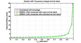
(a) System with 10 queues.

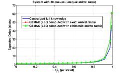
(b) System with 30 queues.

Figure 6: Performance of QZMAC with exact and estimated arrival rates ($T_{p}=3$ and $T_{c}=7$).

VII-B Mean Delay Performance of QZMAC

With Bernoulli arrivals to each queue, the centralized full knowledge scheduler converts the system into a $Geo^{[x]}/D/1$ queue. In every slot, the arrivals to this queue are distributed according to a Binomial$(N,\lambda)$ distribution, where $\lambda\in[0,1/N)$ is the common arrival rate to all queues. This queue can be analyzed for expected delay, and we get $W(\lambda)=\frac{2-(N+1)\lambda}{2(1-N\lambda)}$.

We first consider a system with equal arrival rates and compare the performance of QZMAC and EZMAC with that of ZMAC and the $Geo^{[X]}/D/1$ queue ($W(\lambda)$). We see from figures 7(a) and 7(b), that the delay achieved by QZMAC is very close to optimal as is that achieved by EZMAC (although slightly worse than QZMAC). In Fig. 7(a), the $Geo^{[x]}/D/1$ queue delay cannot be seen explicitly since QZMAC performs almost exactly like it. This is quite encouraging since QZMAC only needs knowledge of the time since a queue was served last, while the optimal algorithm needs full queue-length knowledge at all times. With $30$ queues, in fact, QZMAC shows a decrease in delay over ZMAC of more than $60\%$ and EZMAC of more than $40\%$.

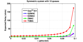
(a) System with 10 queues.

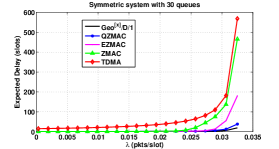
(b) System with 30 queues.

Figure 7: Expected delay with QZMAC, ZMAC and EZMAC. The systems have 10 queues 7(a) and 30 queues 7(b). $T_{c}=9$ for ZMAC and $8$ for EZMAC. For QZMAC, $T_{c}=7$.

Note that since QZMAC requires $T_{p}=3$, in order to keep the scheduling portion’s length $T_{c}+T_{p}$ constant so as to maintain the scheduling portion to transmission portion (see Fig. 3) fraction uniform across protocols, we have reduced the contention window size by three minislots while simulating QZMAC. Also, as the first figure shows, for low and moderate arrival rates, in small WSNs one can use EZMAC and still achieve good delay performance.
We computed the empirical cumulative distribution functions (CDFs) of system backlog with all three protocols (and basic TDMA as an upper bound). As Fig. 8 clearly shows, QZMAC indeed provides the stochastically smallest sum queue lengths. With QZMAC, the CDF hits $1$ at $12$ packets, while its closest competitor, EZMAC’s CDF has a support that extends until $69$ packets and that of ZMAC extends to $220$ packets.

Figure 8: The CDFs of total system backlog with QZMAC, EZMAC, ZMAC, TDMA and the $Geo^{[x]}/D/1$ queue.

VII-C Tuning QZMAC

One can tune QZMAC by changing $T_{p}$ and $T_{c}$ keeping $T_{p}+T_{c}=c$, a constant. As the number of slots reserved for polling ($T_{p}$) increases, Fig. 9 shows that QZMAC with small $T_{p}$ initially performs better, but at high loads, is overtaken by QZMAC with small $T_{c}.$ At arrival rates close to $0$ (i.e., $\lambda\approx 0$), it is an SU that transmits during most slots. This is because, with high probability, the PU’s are empty and the protocol enters the contention portion. Clearly, higher the value of $T_{c}$, greater the probability of resolving this contention. But at high loads ($\lambda\approx\frac{1}{N}$) the PU’s are nonempty with high probability and hence, the polling portion is more likely to yield a nonempty queue. With a higher value of $T_{p}$, a nonempty queue can be found and the system does not have to go into contention. This trend is expected and opens up avenues for further research about protocols that automatically choose the right $T_{c}$ and $T_{p}$.

Figure 9: Figure showing how QZMAC can be tuned. Keeping $T_{p}+T_{c}$ fixed at $10$ minislots, increasing $T_{p}$ causes delay to increase at light loads and decrease at heavy loads.

VII-D Channel Utilization

Recall from our earlier discussion (see Prop. 1) that the optimal scheduling policy under the information structure assumed in this paper lies in the class of non-idling, exhaustive policies. Consequently, the more efficiently a MAC algorithm finds nonempty queues in the network (assuming there are packets in the network), the better its mean delay performance is likely to be. In the literature, this probability of a nonempty queue being served when one exists in the network is termed Channel Utilization, ($\zeta$) and is a performance metric commonly used to compare the efficiency of MAC algorithms [15, 18]. Formally, given a scheduling policy $\pi,$

$$\zeta^{\pi}(\mathbf{Q}(0)) := \lim_{t\rightarrow\infty}\mathbb{P}^{\pi}_{\mathbf{Q}(0)}\left(\sum_{j=1}^{N}\mathbb{I}_{\{Q_{j}(t)>0\}}D_{j}(t)>0\bigg{|}\sum_{j=1}^{N}Q_{j}(t)>0\right)$$

$$\stackrel{{\scriptstyle(*)}}{{=}} \lim_{t\rightarrow\infty}\frac{\sum_{s=0}^{t-1}\sum_{j=1}^{N}\mathbb{I}_{\{Q_{j}(s)>0\}}\mathbb{I}_{\{D_{j}(s)>0\}}}{\sum_{s=0}^{t-1}\mathbb{I}_{\{\sum_{j=1}^{N}Q_{j}(s)>0\}}},$$

where the $(*)$ is under the assumption that the queue length process is ergodic. We used the setup described in Sec. IX-A, to compare the channel utilization of QZMAC with that of ZMAC. The network comprised 7 collocated nodes transmitting to a base station. Packet arrivals to the nodes followed i.i.d Bernoulli processes with rates $\boldsymbol{\lambda}=[0.17,0.20,0.04,0.17,0.17,0.02,0.07]$. This rate vector is clearly within the network capacity region, because $\sum_{i=1}^{7}\lambda_{i}=0.84<1$. The results of the experiment are shown in Table. I. The experiment was repeated for different values of control overhead, i.e., the portion of the time slot wasted in scheduling a queue ($T_{p}+T_{c}$). The value of $T_{p}$ was kept constant, $T_{p}=1$ for ZMAC and $T_{p}=3$ for QZMAC, and the number of contention minislots was varied.

One obvious trend is that channel utilization increases as control overhead increases, since it becomes easier to resolve contention whenever it occurs with more $T_{c}$ minislots. However, the other point to note is that regardless of contention overhead, QZMAC outperforms ZMAC. This is due to the fact that both the polling and the contention mechanisms of the former are designed better than the latter to find nonempty queues with greater probability.

Algorithm	$T_{p}+T_{c}=7$	$T_{p}+T_{c}=8$	$T_{p}+T_{c}=9$
ZMAC ($T_{p}=1$)	0.88968	0.90379	0.91356
QZMAC ($T_{p}=3$)	0.96312	0.9706	0.97486

TABLE I: Comparing the channel utilization of QZMAC with that of ZMAC with varying control overhead ($T_{p}+T_{c}$). Clearly, $\zeta^{QZMAC}>\zeta^{ZMAC}$, showing that the former wastes the channel less often, thereby clearing the network of packets more efficiently.

VIII Conclusion and Future work

In this paper, we first derived optimal polling policies for systems with limited information structures and proved the delay-optimality of exhaustive service and cyclic polling in a symmetric version of our scheduling problem. Leveraging these results, we proposed two distributed protocols QZMAC and EZMAC that perform much better than those available in the literature, both with respect to mean delay and system backlog distributions. We then implemented QZMAC on a test bed comprising telosB motes and demonstrated the operation of several salient aspects of the protocol. Extensions to this work can include the inclusion of Markovian arrivals, channel fading, extension to noncollocated nodes, and sleep-wake cycling sensor nodes.

IX Appendix

IX-A Experiments on an Implementation of QZMAC

We implement the QZMAC algorithm as an additional module in the MAC layer of the 6TiSCH communication stack under the Contiki operating system [30]. With the aid of in-built Contiki-based APIs, we implemented different wireless transceiver functionalities and carried out our experiments over Channel 15 of the 2.4 GHz ISM band. We deployed CC2420 based telosB motes placed equidistant from the receiver node on a circular table Fig. 10. Here, the node placed in the center acts as a “Border Router” (BR), more commonly known as a “Sink.” The BR is always connected to a PC (host) through a USB cable; the BR collects the data packets from the sensor nodes and sends them to the host, which can further route them to the data processing computer over the Internet. Nodes labeled $1$ to $4$ in Fig. 10 are the sensor nodes upon which QZMAC runs.

Figure 10: The center node is the Border Router (sink) and the other nodes, numbered 1 to 4, are the sensor nodes. The sensors are programmed to run QZMAC and transmit packets to the sink.

Our experiments aim to study the following aspects: (a) The network infers and maintain the status of $\mathbf{V}$ vector based on empty and nonempty status of sensor nodes, (b) Verify the protocol working in contention mode as described between step 25 and step 33 of the QZMAC, (c) CCA status inference across the slots, and (d) Synchronization within the network.

IX-B Frame Structure: Time Slots and Mini-Slots

Time Slotted Channel Hopping (TSCH) is a MAC layer specified in the IEEE 802.15.4-2015 [31] standard, with a design inherited from WirelessHART and ISA 100.11a standards. In our implementation, we used the slots defined as part of TSCH within Contiki (sans the channel hopping utility). The duration of a time slot is $15ms$ which is sufficiently long for the transmitter to transmit the longest possible packet and for the receiver to return an acknowledgment.
The slots are further divided into polling minislots and contention minislots as shown in Fig. 3. The minislots are of two standard Clear Channel Assessment (CCA) duration, where $1$ CCA duration is $128$ microseconds. In our experiments, we used $T_{p}=3$, and $T_{c}=9$.

IX-C Time Synchronization

Maintaining network-wide time synchronization at the level of the minislots is a nontrivial problem. For our experiments, we used the Adaptive Synchronization Technique [32]. The Border Router periodically broadcasts Enhanced Beacons (EBs) containing a field indicating the current slot number also known as Absolute Slot Number (ASN). The other nodes store the ASN value and increment it every slot to keep the time slot number aligned. To align the time slot boundaries, the first mini-slot begins after a guard time offset of TsTxOffset from the leading edge of every slot. Every node timestamps the instant it starts receiving the EB, and then aligns its internal timers so that its slot starts exactly TsTxOffset before the reception of EB. In our implementation we used TsTxOffset=$1.8$ms. Through extensive experimentation, we verified that clock drifts were not affecting the protocol’s working across the minislots. The nodes form a $1$-hop fully connected network. We used the “Routing Protocol for Low-Power and Lossy Links” (RPL) to form the routes within the network [33] and verified the working of our firmware on the COOJA simulator [34], before compiling it on to real target motes. We now describe our methodology in detail.

IX-D CCA Errors : Inference and Handling

To study the effect of CCA errors on our protocol, we set up two testbeds (similar to the one in Fig. 10) with network diameter $6$ meters and $8$ meters respectively, each running QZMAC for a period of 12 hours (i.e., $3\times 10^{6}$ time slots). The sensor nodes were programmed to generate packet at constant rate ensuring the queue at sensor nodes are always nonempty and transmit as per the protocol. One of the sensor nodes was connected to a terminal and designated to monitor the CCA status during the experiment. Over the course of our experiment, we observed $1$ CCA “Miss” error on the testbed with $6$ m network diameter and, on the network with $8$ m diameter, we recorded $3$ CCA “Miss” errors, both calculated over a period of 12 hours. No False Alarms were observed. Further, in any given time-slot at most one CCA error occurred network-wide.

Avinash Mohan (S.M. ’16, M ’17) obtained his MTech from the Indian Institute of Technology (IIT) Madras, and PhD from and the Indian Institute of Science (IISc) Bangalore, in 2010 and 2018 respectively. He was a postdoctoral fellow with the Reinforcement Learning Research Labs ($(RL)^{2}$) at the Technion, Israel Institute of Technology, Haifa, Israel and is currently with The Boston University, Massachusetts, USA. His research interests include reinforcement learning, stochastic control, analysis of deregulated energy markets and resource allocation in wireless communication networks.

Arpan Chattopadhyay obtained his B.E. in Electronics and Telecommunication Engineering from Jadavpur University, India in 2008, and M.E. and Ph.D in Telecommunication Engineering from Indian Institute of Science, Bangalore, India in 2010 and 2015, respectively. He is currently working as an Assistant Professor with the Electrical Engineering Department, IIT Delhi. Previously, he held postdoctoral positions with the Electrical Engineering Department, University of Southern California, and INRIA/ENS Paris. His research interests include wireless communication and networks, cyber-physical systems, networked estimation and control, and reinforcement learning.

Shivam Vinayak Vatsa (B Tech. ’16) obtained Bachelor of Technology from NIIT University, India in Computer Science. He is currently a Project Associate II at Center for Networked Intelligence, Indian Institute of Science, Bangalore, India. In past, he worked as Software Engineer in Common Algorithm Development Group at ABB India. His research interests include Internet of Things, Cyber Physical Systems and Data analysis of wireless communication networks.

Anurag Kumar (B.Tech., Indian Institute of Technology (IIT) Kanpur; PhD, Cornell University, both in Electrical Engineering) was with Bell Labs, Holmdel, N.J., for over 6 years. Since then he has been on the faculty of the ECE Department at the Indian Institute of Science (IISc), Bangalore; he was the Director of the Institute during 2014-2020, and now holds an emeritus position. His area of research has been communication networking, and he has recently focused primarily on wireless networking. He is a Fellow of the IEEE, the Indian National Science Academy (INSA), the Indian National Academy of Engineering (INAE), the Indian Academy of Sciences (IASc), and The World Academy of Sciences (TWAS). He was an associate editor of IEEE Transactions on Networking, and of IEEE Communications Surveys and Tutorials.

X Supplementary Material

X-A Glossary of Notation and Acronyms

1. $A_{j}(t)$: number of packets arriving to Queue $j$ in time slot $t.$

2. $B(V_{j})$: If $A$ is a generic Bernoulli($\lambda$) random variable, and $C$ is distributed Binomial($V_{j},\lambda$), then $B(V_{j})$ is a random variable whose distribution is the same as that of $(C-1)^{+}+A$.

3. : Carrier Sense Multiple Access

4. CCA: Clear Channel Assessment.

5. $D_{j}(t)$: the number of departures from Queue $j$ in time slot $t.$

6. DRAND: Distributed RAND (distributed implementation of the RAND protocol)

7. $Geo^{[x]}/D/1$ queue: has arrivals that are sums of Bernoulli random variables (here, $N$), and has a single server (hence, the “$1$”), whose service times are deterministic (hence, the “$D$”).

8. $H^{\pi}_{t}$: the history of policy $\pi$ up to time $t$ as defined in (3).

9. $\mathbf{Q}(t)$: backlog of Queue $j$ at the beginning of time slot $t.$

10. $Q^{\pi}_{j}(t)$: backlog of Queue $j$ at the beginning of time slot $t$ under scheduling policy $\pi.$

11. $K_{thr}$: the threshold that triggers the RESET subroutine. It is denoted by THRSLD in the subroutine description.

12. $\boldsymbol{\lambda}$: the arrival rate vector.

13. $\boldsymbol{\Lambda}$: the capacity region of the queueing network.

14. $\boldsymbol{\Lambda}_{LEQ}$: the set of arrival rates that the LEQ policy can stabilize.

15. $[N]$: the set of integers $\{1,2,\cdots,N\}$.

16. NDST: is short for “Node State.” Attains values COLL (meaning “in collision”) or NOCOLL (meaning “not in collision”).

17. PU: Primary User.

18. $\Pi$: the space of all admissible policies.

19. $\Pi_{e}$: the subset of all exhaustive service policies.

20. $\Pi_{g}$: the subset of all non-idling service policies.

21. RSTBCN: Reset Beacon.

22. SU: Secondary User. In ZMAC this refers to any queue which is not the current PU. In EZMAC and QZMAC, this refers to the queue that won the latest contention.

23. $T_{c}$: number of minislots reserved for contention.

24. TDMA: Time Division Multiple Access

25. $T_{p}$: number of minislots reserved for polling.

26. $V^{\pi}_{j}(t)$: is the number of slots prior to slot $t$ in which Queue $j$ was allowed to transmit under a generic scheduling policy $\pi$.

X-B Terminology Related to MAC Protocol Analysis

We provide brief explanation for some standard terminology related to the analysis of MAC protocols. For further details, the reader can refer to “Multiple access protocols: performance and analysis,” by R. Rom and M. Sidi, Springer-Verlag New York, 1990.

• Backlog: at time $t+,$ i.e., the beginning of slot $t,$ the number of packets in Queue $j$ is called its “backlog,” and is denoted by $Q_{j}(t).$

• Stochastic dominance: given two random variables $X$ and $Y,$ we say that $X$ “stochastically dominates” $Y$ if, $\forall q\in(-\infty,\infty),$ $P(X\leq q)\leq P(Y\leq q).$

• Stochastic ordering: two random variables $X$ and $Y$ are said to be “stochastically ordered”, if either $X$ stochastically dominates $Y,$ or vice versa.

• Switchover delay: informally, this is the amount of time the server takes to stop service at one queue and begin service at a different queue.

• Overhearing: when wireless devices communicate using a shared medium, such as in a wireless network, due to the nature of wireless communication, it is possible for nearby devices to receive signals that are intended for other devices. This unintentional reception of signals is known as overhearing.
  Wireless transmissions are typically encrypted to prevent decoding through overhearing. In our paper, however, we take advantage of overhearing to simply detect the presence of an ongoing transmission (the eavesdropping device does not attempt to decode anything).

X-C Proof of Prop. 1

This proof proceeds along the lines of the proof in [19, Prop. 4.2]. It is easy to show that we can restrict attention to non-idling policies and so, we begin our proof with some policy $\pi\in\Pi_{g}$, where, as mentioned in Sec. III-B, $\Pi_{g}$ is the set of all non-idling policies. Consider a sample path $\omega$ $\left(\right.$a realization of the input sequences $\left.\left\{A_{i}(n)\right\}_{n=1}^{\infty},i\in I\right)$ and on that path, let

$$n^{*}:=\inf\left\{n\geq 1:Q^{\pi}_{\pi^{q}_{n-1}}(n)>0,~{}Q^{\pi}_{\pi^{q}_{n}}(n)=0,~{}\text{and}~{}\pi^{a}_{n}=2\right\}.$$ (13)

This is the first instant when a time slot is wasted by $\pi$ on account of switching to an empty queue though the previous one was non-empty. Further define

$$m^{*}=\inf\left\{n>n^{*}:Q^{\pi}_{\pi^{q}_{n-1}}(n)>0,\pi^{q}_{n-1}=\pi^{q}_{n^{*}},~{}\text{and}~{}\pi^{a}_{n}=1\right\}.$$ (14)

This is the first time since $n^{*}$ that the server continues to serve the (same) incumbent finding it to be non-empty.

Figure 11: A sample path illustrating how $\gamma$ is derived from $\pi$.

Construct another policy $\gamma$ as follows (refer to Fig.11 for an illustration).

• On $[1,n^{*})$ and $[m^{*}+1,\infty)$, $(\gamma^{a}_{k},\gamma^{q}_{k})=(\pi^{a}_{k},\pi^{q}_{k})$.

• $(\gamma^{a}_{n^{*}},\gamma^{q}_{n^{*}})=(1,\pi^{q}_{(n^{*}-1)})$, and

• for $n^{*}+1\leq k\leq m^{*}$, $(\gamma^{a}_{k},\gamma^{q}_{k})=(\pi^{a}_{k-1},\pi^{q}_{k-1})$.

So, $\gamma$ follows $\pi$ over $[1,n^{*})$ and $[m^{*}+1,\infty)$ and at $n^{*}$, $\gamma$ deviates from $\pi$ and serves the incumbent (possible, since that queue is non-empty). Between $n^{*}+1$ and $m^{*}$, $\gamma$ follows $\pi$ albeit with one slot delay, i.e., it does whatever $\pi$ did one slot ago. Clearly,

$$Q^{\gamma}(t)=Q^{\pi}(t),~{}\forall~{}t\in[1,n^{*})\cup[m^{*}+1,\infty),~{}\text{and}$$

$$Q^{\gamma}(t)\leq Q^{\pi}(t),~{}\forall~{}t\in[n^{*}+1,\leq m^{*}],\hskip 28.45274pt$$

whenever $m^{*}<\infty$. This relation is true for every sample path $\omega$. $m^{*}$ is set equal to $\infty$ whenever either $n^{*}=\infty$, or, $\gamma$ is able to serve a packet in some slot $l$ ($\geq n^{*}+1$) while $\pi$ could not serve any packet in slot $l-1$.

To explain the latter case further, observe that after $n^{*}$, $\gamma$ does whatever $\pi$ did one slot ago. If $\pi$ switched to some empty queue in $l-1$, $\gamma$ switches to the same queue in $l$. But if $\pi^{q}_{l-1}$ received a packet in $l-1$, $\gamma$ will be able to serve that packet increasing $Q^{\pi}(t)-Q^{\xi}(t)$ to 2 (one at $n^{*}$ and the second at $l$). Since $\gamma$ follows $\pi$ with exactly one step delay, $\pi$ will never be able to make up the difference! Hence, $m^{*}=\infty$.

To complete the proof, one needs to consider epochs $l^{*}$ such as:

$$l^{*} := \inf\{n\geq 1:Q^{\pi}_{\pi^{q}_{n-1}}(n)>0,Q^{\pi}_{\pi^{q}_{n}}(n)>0,$$ (15)

$$\text{and}~{}\pi^{a}_{n}=2\},$$

wherein the queue which $\pi$ decides to serve, unlike the case with $n^{*}$, is non-empty and hence, slot $l^{*}$ is not wasted. Even in this case defining $\gamma$ as before produces a policy that does no worse than $\pi$ in terms of total system backlog.

In the same manner, find such an $n^{*}$ (or $l^{*}$ as the case may be) for $\gamma$ and refine this policy using the procedure described. Iterating this procedure, one ends up with a policy say $\xi$, for which such an instant never exists, i.e., which never switches to a different queue when the incumbent is nonempty. This is by definition exhaustive. We have, thus, defined both queueing processes on some common probability space $\left(\Omega,\mathcal{F},\mathbb{P}\right)$ and for every $\omega\in\Omega$, we have shown that

$$Q^{\xi}(t,\omega)\leq Q^{\pi}(t,\omega),~{}\forall~{}t\geq 1,$$

which means that $\forall x\in\mathbb{R}$,

$$\mathbb{P}\{\omega:Q^{\pi}(t,\omega)>x\}\geq\mathbb{P}\{\omega:Q^{\xi}(t,\omega)>x\}.$$ (16)

This coupling argument shows that

$$Q^{\xi}(t)\stackrel{{\scriptstyle st}}{{\leq}}Q^{\pi}(t),~{}\forall~{}t\geq 1.$$ (17)

∎

X-D Longest Expected Queue (LEQ) and Stochastically Largest Queue (SLQ) Policies

Let the arrival rate vector be denoted by $\boldsymbol{\lambda}$ ($\in\mathbb{R}^{N}_{+}$). For notational convenience, in the sequel, we denote the number of slots since Queue $i$ was last served, formerly denoted $V_{i}^{\pi}(t)$, by $V_{i}(t)$ (omitting the policy superscript). Since we consider exhaustive service, $\lambda_{i}V_{i}(t)$ is the expected backlog of queue $i$ at $t$, and $arg~{}max_{1\leq i\leq N}\lambda_{i}V_{i}(t)$ is the longest expected backlog. We call the policy that, at every scheduling instant, schedules this queue the Longest Expected Queue (LEQ) policy.

Remark.

1. Comparing the definition of the region $\Lambda_{LEQ}$ with that of the region $\Lambda$ in Eqn. 2 shows quite clearly, that the LEQ policy is throughput optimal.

2. With $\lambda_{i}=\lambda,\forall i$, we have and the policy is easily seen to be a cyclic exhaustive policy, i.e., queues are served in a fixed cycle, with each queue being served to exhaustion. $arg~{}max_{1\leq i\leq N}\lambda_{i}V_{i}(t)=arg~{}max_{1\leq i\leq N}V_{i}(t)$ and the policy reduces to a cyclic exhaustive service policy.

LEQ vs SLQ. Note that when $V_{l}\neq V_{k}$ and $\lambda_{l}\neq\lambda_{k},$ it might not even be possible to stochastically order random variables distributed according to Binomial($V_{l},\lambda_{l}$) and Binomial($V_{k},\lambda_{k}$). An example is when $V_{l}>V_{k}$, but $\lambda_{l}<\lambda_{k}.$ Hence, with unequal arrival rates, the LEQ policy doesn’t necessarily choose the stochastically longest queue, but only the queue with the largest mean backlog. This is the difference between the LEQ and SLQ policies. In the sequel, we denote the set of all SLQ policies by $\Pi_{s}$.

Recall that under symmetry, the LEQ policy essentially schedules $arg~{}max_{1\leq i\leq N}V_{i}(t)$ at every scheduling instant and exhaustively serves this queue. Why exhaustive service? As an example, Consider the scenario with 4 queues in the system and suppose that at the beginning of Queue $1$'s service, $\mathbf{V}=[0,v_{2},v_{3},v_{4}]$, with $v_{2}>v_{3}>v_{4}$. At the end of Queue $1$'s service, the vector changes to $\mathbf{V}^{\prime}=[0,v_{2}^{\prime},v_{3}^{\prime},v_{4}^{\prime}]$, but the ordering is still preserved, i.e., $v^{\prime}_{2}>v^{\prime}_{3}>v^{\prime}_{4}>v^{\prime}_{1}=0$. Hence, Queue 2 is chosen for service next. But at the end of queue 2's service, once again, we see that $v^{\prime\prime}_{3}>v^{\prime\prime}_{4}>v^{\prime\prime}_{1}$, as it was at the beginning of Queue 2's service, and Queue 3 is chosen, after which queue 4 is chosen followed by queue 1 and this process repeats. We see that under symmetry, LEQ induces a cyclic service system. This policy is discussed in detail in Sec. III-D. where we will, in fact, show it to be mean delay optimal in symmetric systems. This also helps bolster our confidence in the LEQ policy itself. We now explore in greater detail the behavior of the LEQ policy in symmetric systems.

To prove this we invoke Theorem (3.1) in [35] that proves the stability of certain exhaustive service policies with state dependent routing. We first require some more notation.

We denote by $S(t)$ the queue in service during slot $t$, and set $S(t)=0$ if the server is idling at some queue (which from Prop. 1, has to be empty) during some slot. We denote by $W_{n}$, the time taken by the server to begin the $n^{th}$ service. By this we mean the time taken by the server to find a non empty queue after serving some queue. So, if the incumbent is non empty, $W_{n}=0$ since the server simply begins serving the next packet in the queue served in the previous slot without switching away from it. Otherwise the server begins to search for a non empty queue to begin a busy period. Specifically, if $Q_{S(0)}(0)=0$, then $W_{1}$ is the time taken to find a non empty queue. During this period, the server may have visited several empty queues.

Assume the underlying probability space is denoted by $\left(\Omega,\mathcal{F},P\right)$ and let

$$\mathcal{F}_{n}:=\sigma\left(\bigg{\{}\left[Q_{1}(t),\cdots,~{}Q_{N}(t),~{}S(t)\right],~{}t\leq n\bigg{\}}\right),~{}n\geq 0,$$

be the filtration describing the history of the system. Let $A_{i}[t]$ be the number of arrivals to queue $i$ until and including time $t$, and $A[t]=\sum_{i=1}^{N}A_{i}[t]$, the total number of arrivals to the system over the same duration.

The proof of Theorem (3.1) in [35] relies on two assumptions that we show are satisfied in our case. Firstly, that there exists $w>0$ such that

$$\mathbb{E}\left[W_{1}|\mathcal{F}_{0}\right]<w,~{}P-a.s.~{}\text{on}~{}\left\{Q_{S(0)}=0\right\},$$ (19)

and secondly that there exists some $p>0$ such that

$$P\left(A(W_{1})=0|\mathcal{F}_{0}\right)>p,~{}P-a.s.~{}\text{on}~{}\left\{Q_{S(0)}=0,\sum_{i=1}^{N}X_{i}(0)>0\right\}.$$ (20)

In other words, (19) means that if the system starts out empty, the time taken to find a non empty queue under the policy being considered, should have a finite mean. (20), on the other hand, refers to the fact that when the system starts off non empty and the server is at an empty queue at time $0$, the probability of $0$ arrivals in $W_{1}$ is positive.

First note that on $\{Q_{S(0)}=0\}$, $W_{1}\geq 1$, and let $\lambda_{min}=\min_{1\leq i\leq N}\lambda_{i}$ be the smallest arrival rate which, by assumption is strictly positive. The first assumption is satisfied, since

$$\mathbb{E}\left[W_{1}|\mathcal{F}_{0}\right] = \sum_{k=1}^{\infty}P\{W_{1}\geq k|\mathcal{F}_{0}\}$$

$$\stackrel{{\scriptstyle(*a)}}{{\leq}} \sum_{k=1}^{\infty}(1-\lambda_{S(k)})^{k}$$

$$\leq \sum_{k=1}^{\infty}(1-\lambda_{min})^{k}$$

$$= \frac{1}{\lambda_{min}}-1<\infty.$$

Inequality $(*a)$ is true, since, for the walking time to be at least $k$, the $k^{th}$ polled queue, i.e., $S(k)$, must be empty. Since on $\{Q_{S(0)}=0\}$ the system also starts off empty, this probability is $(1-\lambda_{S(k)})^{k}$. To prove (20), first define $p_{k}=P\{W_{1}=k|\mathcal{F}_{0}\}$.

$$P\{A(W_{1})|\mathcal{F}_{0}\} = \sum_{k=1}^{\infty}P\{A(k)=0|\mathcal{F}_{0},W_{1}=k\}P\{W_{1}=k|\mathcal{F}_{0}\}$$

$$= \sum_{k=1}^{\infty}P\{A(k)=0|\mathcal{F}_{0},W_{1}=k\}p_{k}.$$

$$= \sum_{k=1}^{\infty}\left(\sum_{i=1}^{N}\left(1-\lambda_{i}\right)^{k}\right)p_{k}.$$

But on $\{X_{S(0)}=0\}$, $p_{1}>(1-\lambda_{min})~{}a.s.$ So,

$$P\{A(W_{1})|\mathcal{F}_{0}\} = p_{1}\sum_{i=1}^{N}\left(1-\lambda_{i}\right)$$

$$+\sum_{k=2}^{\infty}\left(\sum_{i=1}^{N}\left(1-\lambda_{i}\right)^{k}\right)p_{k}$$

$$\geq \sum_{i=1}^{N}(1-\lambda_{i})>0.$$

With both (19) and (20) satisfied, we note that Theorem (3.1) in [35] is proved under a much more general model, where the behavior of the system is influenced by another process $U(t),t\geq 0$, that takes values in some measurable space $\left(\mathbf{U},\mathcal{U}\right)$. Setting $\mathbf{U}=\mathbb{N}^{N}$ and $U(t)=V(t)$, the proof is complete.

∎

X-E LEQ with Equal Arrival Rates

With equal arrival rates, $arg~{}max_{1\leq i\leq N}\lambda_{i}V_{i}(t)=arg~{}max_{1\leq i\leq N}V_{i}(t)$ and the policy reduces to a cyclic exhaustive service policy, as can be seen from the following example. Consider the scenario with 4 queues in the system and suppose that at the beginning of Queue $1$'s service, $\mathbf{V}=[0,v_{2},v_{3},v_{4}]$, with $v_{2}>v_{3}>v_{4}$. At the end of Queue $1$'s service, the vector changes to $\mathbf{V}^{\prime}=[0,v_{2}^{\prime},v_{3}^{\prime},v_{4}^{\prime}]$, but the ordering is still preserved, i.e., $v^{\prime}_{2}>v^{\prime}_{3}>v^{\prime}_{4}>v^{\prime}_{1}=0$. Hence, Queue 2 is chosen for service next. But at the end of queue 2's service, once again, we see that $v^{\prime\prime}_{3}>v^{\prime\prime}_{4}>v^{\prime\prime}_{1}$, as it was at the beginning of Queue 2's service, and Queue 3 is chosen, after which queue 4 is chosen followed by queue 1 and this process repeats. We see that under symmetry, LEQ induces a cyclic service system. This policy is discussed in detail in Sec. III-D. where we will, in fact, show it to be mean delay optimal in symmetric systems. This also helps bolster our confidence in the LEQ policy itself. We now explore in greater detail the behavior of the LEQ policy in symmetric systems.

X-F Stability of Cyclic Exhaustive Service

We know that cyclic exhaustive service shows optimal mean delay performance in systems with equal arrival rates. In this section, we make an important observation about its stability in systems with general arrival rates, i.e., not necessarily equal.
The cyclic exhaustive service policy is throughput optimal. The proof of the stability of the cyclic exhaustive service policy proceeds along the lines of the analysis in [36]. Note, however, that the stability of this policy is proved for a system with general (possibly unequal) arrivals rates $\lambda_{1},\cdots,\lambda_{N}$, and includes, as a special case, the stability of the symmetric system. Formally,

Theorem 5.

Consider the system capacity region defined in Eqn. (2). If $\boldsymbol{\lambda}\in\Lambda$, the system is stable under cyclic exhaustive service.

Proof:

The proof involves showing that the drift of a Lyapunov function computed at the end of $N$ busy periods, i.e., between two successive returns to any queue $i$, is negative. Refer to Sec. X-G for details. ∎

Remark.

Although we motivated cyclic exhaustive service as the LEQ policy specialized to symmetric systems, Thm. 5 shows that the former can actually stabilize unequal arrival rates as well. So we now have two throughput optimal scheduling policies (LEQ and cyclic exhaustive service). But since the LEQ policy requires estimates of the arrival rate vector and cyclic exhaustive service does not, can we do away with LEQ altogether? As Fig. 12 shows, with unequal arrival rates, LEQ can deliver substantially better delay performance and hence, is preferable to cyclic exhaustive service. In Sec. VII, we show how LEQ can be implemented in a distributed manner using arrival rate estimation, but where such estimation cannot be performed or is undesirable, cyclic exhaustive service can still be used to stabilize the system albeit at the cost of increased delay.

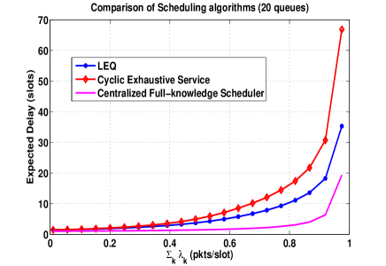
Figure 12: Comparison of the performance of the LEQ and Cyclic Exhaustive Service policies. Also shown is the lowest possible delay achievable in this system (black curve). This is discussed in detail in Sec. VI. We assume a fixed ratio of packet rates that determines the arrival to each queue. Specifically, $r_{i}\lambda$ is the arrival rate to Queue $i$ with $\sum_{i=1}^{N}r_{i}=1$. In the plot, $\lambda\in[0,1)$.

X-G Proof of Thm. 5

In this section, we return to the system discussed Sec.II, i.e., one that is not necessarily symmetric. The analysis proceeds along the lines of the proof of the theorem in [36]. We will be looking at the system’s state only at the epochs at which the server begins its visit to a queue.

With a slight abuse of notation, we define this system’s state is by $\mathbf{s}(n)=\left[\mathbf{Q}(n),I(n)\right]^{T}$, where, $\mathbf{Q}(n)=\left[Q_{1}(n),~{}Q_{2}(n),\dots,Q_{N}(n)\right]^{T},n\geq 1$ is the vector of queue lengths at the $n^{th}$ switching instant (at which the server visits the $n^{th}$ queue), $I(n)$ is the identity of the $n^{th}$ queue polled. Clearly, $\mathbf{s}(n)\in\mathbb{N}^{N}\times I$, and this process is embedded at the instants at which the server arrives at a queue.

Further, the number of arrivals to queue $k$ in $t$ time-slots is denoted by $A_{k}(t)$ and the length of the $n^{th}$ busy period starting with $l$ packets by $G_{n}(l)$. Also,

$$I(n+1)=\begin{cases}I(n)+1~{}~{}\text{if}~{}1\leq n\leq N-1\\ 1\hskip 39.83368pt\text{if}~{}n=N.\end{cases}$$

Consequently, when

1. $j\neq I(n)$

   $$Q_{j}(n+1)=\begin{cases}Q_{j}(n)+A_{j}\left(G_{n}\left(Q_{I(n)}(n)\right)\right),\\ ~{}~{}~{}\text{if}~{}Q_{I(n)}(n)\geq 1\\ Q_{j}(n)+A_{j}(1),\text{if}~{}Q_{I(n)}(n)=0\\ \end{cases}$$

2. $j=I(n)$

   $$Q_{j}(n+1)=A_{j}(1).$$

The mean duration of a busy period, $\mathbb{E}B(I(n))$ of queue $I(n)$ beginning with one packet is found by observing that

$$\mathbb{E}B(I(n)) = \left[1\times\lambda_{I(n)}+\{1+\mathbb{E}G_{n}(l)\}\{1-\lambda_{I(n)}\}\right].$$

$$\Rightarrow\mathbb{E}B(I(n)) = \frac{1}{1-\lambda_{I(n)}}.$$

Hence, since $G_{n}(l)$ begins with $l$ packets instead of one,

$$\mathbb{E}G_{n}(l) = l\times\left[1\times\lambda_{I(n)}+\{1+\mathbb{E}G_{n}(l)\}\{1-\lambda_{I(n)}\}\right]$$ (21)

$$= \frac{l}{1-\lambda_{I(n)}}\hskip 142.26378pt$$

$$\Rightarrow \mathbb{E}A_{j}\left(G_{n}(l)\right)=\frac{\lambda_{j}}{1-\lambda_{I(n)}}l~{}\forall j\neq I(n)$$

$$\Rightarrow \mathbb{E}\sum_{j\neq I(n)}A_{j}\left(G_{n}(l)\right)=\frac{\rho-\lambda_{I(n)}}{1-\lambda_{I(n)}}l.$$

We will now show that $\rho=\sum_{i=1}^{N}\lambda_{i}<1$ is a sufficient condition for stability. Clearly, $\{\mathbf{Q}_{n},n\geq 1\}$, is an irreducible DTMC. However, it is not time homogeneous since, as (21) shows, the transition probabilities depend on the queue being served, i.e., on $I(n)$. Hence, as defined in [36], the system is said to be stable if the $N$ irreducible, homogeneous DTMCs $\{\left[\mathbf{Q}(nN+k),k\right],n\geq 1,1\leq k\leq N,i\in\{1,2\}\}$ are all ergodic.

Now, from the definition of $Q_{j}(n+1)$, we see that

$$\mathbb{E}\left[\sum_{j=1}^{N}Q_{j}(n+1)|\mathbf{Q}(n)\right] \leq \sum_{j=1}^{N}Q_{j}(n)+\rho$$

$$+\frac{\rho-\lambda_{I(n)}}{1-\lambda_{I(n)}}Q_{I(n)}(n)-Q_{I(n)}(n)$$

$$= \sum_{j=1}^{N}Q_{j}(n)+\rho-(1-\rho)h_{I(n)}Q_{I(n)}(n),$$

$$~{}\text{where $h_{I(n)}=\frac{1}{1-\lambda_{I(n)}}$},$$

which means that

$$\mathbb{E}\left[\sum_{j=1}^{N}Q_{j}(n+2)|\mathbf{Q}(n)\right] = \mathbb{E}\left[\mathbb{E}\left[\sum_{j=1}^{N}Q_{j}(n+2)\mid\mathbf{Q}(n+1)\right]\mid\mathbf{Q}(n)\right]$$

$$\leq \mathbb{E}\bigg{[}\sum_{j=1}^{N}Q_{j}(n+1)+\rho$$

$$-(1-\rho)h_{I(n+1)}Q_{I(n+1)}(n+1)\mid\mathbf{Q}(n)\bigg{]}$$

$$\leq \mathbb{E}\bigg{[}\sum_{j=1}^{N}Q_{j}(n+1)\mid\mathbf{Q}(n)\bigg{]}+\rho$$

$$-(1-\rho)h_{I(n+1)}Q_{I(n+1)}(n+1)$$

$$= \sum_{j=1}^{N}Q_{j}(n)+2\rho-(1-\rho)\bigg{[}h_{I(n)}Q_{I(n)}(n)$$

$$+h_{I(n+1)}Q_{I(n+1)}(n)\bigg{]}.$$

Proceeding similarly, we get

$$\mathbb{E}\left[\sum_{j=1}^{N}Q_{j}(n+2N)\mid\mathbf{Q}(n)\right] \leq \sum_{j=1}^{N}Q_{j}(n)+2N\rho$$

$$-(1-\rho)\sum_{m=0}^{2N-1}h_{I(n+m)}Q_{I(n+m)}(n),$$

$$\Rightarrow\mathbb{E}\left[\sum_{j=1}^{N}Q_{j}(n+2N)-\sum_{j=1}^{N}Q_{j}(n)\mid\mathbf{Q}(n)\right]\leq 2N\rho$$

$$-(1-\rho)\sum_{m=0}^{2N-1}h_{I(n+m)}Q_{I(n+m)}(n).$$ (22)

Clearly, the RHS of (22) is at most $2N\rho$, and if for even one $1\leq k\leq 2N$ and $\epsilon>0$, $Q_{I(n+k)}(n)>\frac{N\rho\epsilon}{(1-\rho)h(I(n+k))}$, then $\mathbb{E}\left[\sum_{j=1}^{N}Q_{j}(n+2N)-\sum_{j=1}^{N}Q_{j}(n)\mid\mathbf{Q}(n)\right]<-\epsilon$. Hence, by the Foster-Lyapunov criterion ([20], Thm. 2.2.3), we see that $\{\left[\mathbf{Q}(nN+k),k,i\right],n\geq 1\}$ is positive recurrent for every $1\leq k\leq N$, and $i\in\{1,2\}$. Being irreducible DTMCs as well, it is also ergodic.

∎

X-H Formulating the MDP

1. State Space: The state of the system at time $n\geq 1$ is the vector

   $$s(t)=\left[Q_{u_{n-1}}(n),\mathbf{V}(n),\mathbf{r}(n),u_{n-1}\right].$$ (23)

   So $s(n)\in\mathbb{N}\times\mathbb{N}^{N}\times\mathbb{N}^{N-1}\times I$.

2. Action Space: The action space $\mathbb{A}=I$ for all states.

3. Initial distribution on the State Space: We assume that the system begins empty and so, the initial distribution $D$ is simply $\mathbb{I}\{s(0)\}$, where $s(0)=\left[q,\mathbf{V}(0),\mathbf{r}(0),i_{0}\right],$ is given and hence, known.

4. History: Since the state is observable, the initial history is nothing but the initial state, which is supplied as the initial information.

   $$h_{0}=s(0).$$ (24)

   At time $t$, the history provides the complete picture of successive observations and control actions chosen so far; for $n\geq 1$:

   $$h_{n}=\left(s(0),a(0),\dots,s(n-1),a(n-1),s(n)\right),$$ (25)

   where the action taken at time $n$, $a(n)\in\mathbb{I},\forall n\geq 0.$

5. Policies: In general, a policy is a sequence of conditional distributions $\xi=\{\xi_{n}\}$ such that for each $n$, $\xi_{n}$ is a distribution on $\mathbb{A}$ given $h_{n}$. As mentioned before, we restrict attention to policies that serve any queue $j$ with $r_{j}(t)>0$ first and then return to serve the incumbent. As a consequence of Prop. 1, we also restrict to the case where if $q>0$ then we serve $i$ again.

6. Transition Law: We denote the current action by $u_{n}$ and distinguish two cases:

   • $r_{i}(n)\geq 1$ for some $i\in I-{u_{n-1}}$. Then,

     $$q_{u_{n}}(s(n),s(n+1)) = \mathbb{I}_{\left\{r_{i}(n+1)=r_{i}(n)-1\right\}}\times$$ (26)

     $$\Pi_{j\neq i}\mathbb{I}_{\left\{r_{j}(n+1)=r_{j}(n)\right\}}\mathbb{I}_{\left\{u_{t}=i\right\}}\times$$

     $$\left(\Pi_{k=1}^{N}\mathbb{I}_{u_{n}}\{V_{k}(n),V_{k}(n+1)\}\right)\times$$

     $$\left(\Pi_{k=1}^{N}q^{\prime}_{u_{n}}(Q_{k}(n),Q_{k}(n+1))\right),\hskip 25.6073pt$$

     where

     $${I}_{u_{n}}\{V_{k}(n),V_{k}(n+1)\}:=\begin{cases}1~{}\text{if}~{}V_{k}(n+1)=V_{k}(n)+1~{}\text{and}~{}k\neq u_{n},\\ 1~{}\text{if}~{}V_{k}(n+1)=V_{k}(n)=0~{}\text{and}~{}k=u_{n},~{}\text{and }\\ 0~{}\text{otherwise},\end{cases}$$

     and

     $$q^{\prime}_{u_{n}}(Q_{k}(n),Q_{k}(n+1)):=\begin{cases}\lambda~{}~{}~{}~{}~{}~{}\text{if}~{}Q_{k}(n+1)=Q_{k}(n)+1\\ ~{}~{}~{}~{}~{}~{}~{}\text{OR, if}~{}Q_{k}(n+1)=(Q_{k}(n)-1)^{+}+1\\ ~{}~{}~{}~{}~{}~{}~{}~{}\text{and }k=i,\\ 1-\lambda~{}\text{if}~{}Q_{k}(n+1)=Q_{k}(n)+0\\ ~{}~{}~{}~{}~{}~{}~{}\text{OR, if}~{}Q_{k}(n+1)=(Q_{k}(n)-1)^{+}+0\\ ~{}~{}~{}~{}~{}~{}~{}~{}\text{and }k=i,\\ 0~{}~{}~{}~{}~{}~{}\text{otherwise},\end{cases}$$

   • $\mathbf{r}(n)=\mathbf{0}$. Then,

     $$q_{u_{n}}(s(n),s(n+1)) = \Pi_{j\in I}\mathbb{I}_{\left\{r_{j}(n+1)=0\right\}}\times$$ (27)

     $$\left(\Pi_{k=1}^{N}\mathbb{I}_{u_{n}}\{V_{k}(n),V_{k}(n+1)\}\right)\times$$

     $$\left(\Pi_{k=1}^{N}q^{\prime}_{u_{n}}(Q_{k}(n),Q_{k}(n+1))\right),\hskip 25.6073pt$$

     where

     $${I}_{u_{n}}\{V_{k}(n),V_{k}(n+1)\}:=\begin{cases}1~{}\text{if}~{}V_{k}(n+1)=V_{k}(n)+1~{}\text{and}~{}k\neq u_{n},\\ 1~{}\text{if}~{}V_{k}(n+1)=V_{k}(n)=0~{}\text{and}~{}k=u_{n},~{}\text{and}\\ 0~{}\text{otherwise},\end{cases}$$

     and

     $$q^{\prime}_{u_{n}}(Q_{k}(n),Q_{k}(n+1)):=\begin{cases}\lambda~{}~{}~{}~{}~{}~{}\text{if}~{}Q_{k}(n+1)=Q_{k}(n)+1~{}\text{and}~{}k\neq u_{n},\\ ~{}~{}~{}~{}~{}~{}~{}\text{OR, if}~{}Q_{k}(n+1)=(Q_{k}(n)-1)^{+}+1\\ ~{}~{}~{}~{}~{}~{}~{}~{}\text{and }k=u_{n},\\ 1-\lambda~{}\text{if}~{}Q_{k}(n+1)=Q_{k}(n)+0~{}\text{and}~{}k\neq u_{n},\\ ~{}~{}~{}~{}~{}~{}~{}\text{OR, if}~{}Q_{k}(n+1)=(Q_{k}(n)-1)^{+}+0\\ ~{}~{}~{}~{}~{}~{}~{}~{}\text{and }k=u_{n},\\ 0~{}~{}~{}~{}~{}~{}\text{otherwise},\end{cases}$$

7. Single Stage Cost: This gives the expected cost over the current step when the current state and action are known.

   $$c(s(n),u_{n}) = \mathbb{E}\left[\sum_{i=1}^{N}Q_{i}(n)|s_{n}\right]$$ (28)

   $$= Q_{u_{n-1}}(n)+\lambda\sum_{j\neq u_{n-1}}V_{j}(n)+\sum_{i\in I}R_{i}(n),\hskip 25.6073pt$$

   which is the expected sum of the current queue lengths conditioned on the current state.

Recall that the optimal cost (Eqn. (9)) is given by

$$J^{*}(s(0))=min_{\xi}~{}\mathbb{E}^{\xi}_{s(0)}\sum_{n=0}^{\infty}\alpha^{n}\mathbb{E}\left[\sum_{i=1}^{N}Q_{i}(n)|s_{n}\right].$$ (29)

It is to be noted that $J^{*}(s(0))$ on the R.H.S of (9) exists for every initial state $s(0)$. Since arrivals are IID Bernoulli variables, the single stage cost can increase at most linearly with time, while the discount factor $\alpha^{n}$ decreases exponentially and dominates.

The Bellman Optimality equations [24] associated with this MDP formulation are as follows (recall from Eqn. (10) that we denote $J^{*}(q;\mathbf{V};\mathbf{r};i)$ by $J_{i}^{*}(q;\mathbf{V};\mathbf{r})$). When $\mathbf{r}=\mathbf{0}$,

$$J^{*}_{i}(q>0;\mathbf{V};\mathbf{r}=\mathbf{0}) = q+\lambda\sum_{k\neq i}V_{k}+\alpha\mathbb{E}J^{*}_{i}\left(q-1+A;\right.$$

$$\left.V_{i}=0,\mathbf{V}_{-i}+\mathbf{1};\mathbf{r}=\mathbf{0}\right),$$

$$J^{*}_{i}(q=0;\mathbf{V};\mathbf{r}=\mathbf{0}) = \lambda\sum_{k\neq i}V_{k}+\alpha\min_{j\neq i}\mathbb{E}J^{*}_{j}\left(B(V_{j});\right.$$

$$\left.V_{j}=0,\mathbf{V}_{-j}+\mathbf{1};\mathbf{r}=\mathbf{0}\right),$$

where $A$ is a generic Bernoulli($\lambda$) random variable, $\mathbf{V}_{-i}=[V_{1},\dots,V_{i-1},V_{i+1},\dots,V_{N}]$ and $\mathbf{1}\in\mathbb{R}^{(N-1)}$ is the vector with 1’s at all coordinates. Finally, if random variable $C$ is distributed Binomial($V_{j},\lambda$), $B(V_{j})$ is a random variable whose distribution is the same as that of $(C-1)^{+}+A$.

If $r_{j}\geq 1$ for some $j\in I-\{i\}$, the server first serves the $\sum_{j\neq i}r_{j}$ packets and then returns to queue $i$. Let $\tilde{R}=\sum_{j\neq i}r_{j}$, $L_{-i}=\sum_{j\neq i}V_{j}$, and $\tilde{L}_{-i}=\sum_{k=1}^{\tilde{R}}\alpha^{(\tilde{R}-k)}(L_{-i}+Nk)$. Clubbing all these $\tilde{R}$ slots, we get:

$$J^{*}_{i}(q>0;\mathbf{V};\mathbf{r}) = q\sum_{k=0}^{\tilde{R}-1}\alpha^{k}+\lambda\tilde{L}_{-i}+\alpha^{\tilde{R}}\mathbb{E}J^{*}_{i}\left(q-1+\tilde{A};\right.$$

$$\left.V_{i}=0,\mathbf{V}_{-i}+\tilde{R}\mathbf{1};\mathbf{r}=\mathbf{0}\right)$$

$$J^{*}_{i}(q=0;\mathbf{V};\mathbf{r}) = \lambda\tilde{L}_{-i}+\alpha^{\tilde{R}}\mathbb{E}J^{*}_{j}\left(\tilde{A};V_{j}=0,\right.$$ (30)

$$\left.\mathbf{V}_{-j}+\tilde{R}\mathbf{1};\mathbf{r}=\mathbf{0}\right),\hskip 21.33955pt$$

where $\tilde{A}$ is a Binomial$\left(\tilde{R},\lambda\right)$ random variable and represents the number of arrivals over $\tilde{R}$ slots.

X-I Proof of Thm. 2

Before we prove that cyclic exhaustive service solves the discounted cost MDP described in Sec. X-H, we require an intermediate result on monotonicity of the optimal cost function.

X-I1 Monotonicity of $J^{*}(\cdot)$

Consider, once again, the Bellman equations.

$$J^{*}_{i}(q>0;\mathbf{v};\mathbf{r}=\mathbf{0}) = q+\lambda\sum_{k\neq i}v_{k}+\alpha\mathbb{E}J^{*}_{i}\left(q-1+A;\right.$$

$$\left.v_{i}=0,\mathbf{v}_{-i}+\mathbf{1};\mathbf{r}=\mathbf{0}\right),$$

$$J^{*}_{i}(q=0;\mathbf{v};\mathbf{r}=\mathbf{0}) = \lambda\sum_{k\neq i}v_{k}+\alpha\min_{j\neq i}\mathbb{E}J^{*}_{j}\left(B(v_{j});\right.$$ (31)

$$\left.v_{j}=0,\mathbf{v}_{-j}+\mathbf{1};\mathbf{r}=\mathbf{0}\right),$$

where, we recall that if random variable $C$ is distributed Binomial($v_{j},\lambda$), $B(v_{j})$ is a random variable whose distribution is the same as that of $(C-1)^{+}+A$ and $A$ is a Bernoulli random variable with $\mathbb{E}A=\lambda$. We shall now prove that the optimal cost function is monotonically increasing in the first coordinate when $\mathbf{r}=\mathbf{0}$ (this is really the only scenario where decisions might have to be taken).

References

- [1] A. Mohan, A. Chattopadhyay, and A. Kumar, “Hybrid MAC protocols for low-delay scheduling,” in Mobile Ad Hoc and Sensor Systems (MASS), 2016 IEEE 13th International Conference on. IEEE, 2016.
- [2] D. Dujovne, T. Watteyne, X. Vilajosana, and P. Thubert, “6tisch: deterministic ip-enabled industrial internet (of things),” IEEE Communications Magazine, vol. 52, no. 12, pp. 36–41, 2014.
- [3] R. Y. Zhong, L. Wang, and X. Xu, “An iot-enabled real-time machine status monitoring approach for cloud manufacturing,” Procedia CIRP, 2017.
- [4] P. Thubert, M. R. Palattella, and T. Engel, “6TiSCH centralized scheduling: when SDN meets IoT,” in IEEE CSCN, 2015.
- [5] S. S. Lam (editor), Principles of Communication and Networking Protocols. IEEE Computer Society Press, 1984.
- [6] L. Jiang and J. Walrand, “Stability and delay of distributed scheduling algorithms for networks of conflicting queues,” Queueing Systems, 2012.
- [7] ——, “Approaching throughput-optimality in distributed csma scheduling algorithms with collisions,” Networking, IEEE/ACM Transactions on, 2011.
- [8] S. Rajagopalan, D. Shah, and J. Shin, “Network adiabatic theorem: an efficient randomized protocol for contention resolution,” in ACM SIGMETRICS Performance Evaluation Review, 2009.
- [9] H. Takagi and L. Kleinrock, “A tutorial on the analysis of polling systems, Tech. Rep. UCLA Report No. 850005, ’85.
- [10] R. A. Nazib and S. Moh, “Energy-efficient and fast data collection in uav-aided wireless sensor networks for hilly terrains,” IEEE Access, vol. 9, pp. 23 168–23 190, 2021.
- [11] Y. Liu, K. Ota, K. Zhang, M. Ma, N. Xiong, A. Liu, and J. Long, “Qtsac: An energy-efficient mac protocol for delay minimization in wireless sensor networks,” IEEE Access, vol. 6, pp. 8273–8291, 2018.
- [12] A. Ephremides, O. Mowafi, et al., “Analysis of a hybrid access scheme for buffered users-probabilistic time division,” Software Engineering, IEEE Transactions on, no. 1, pp. 52–61, 1982.
- [13] C. Doerr, M. Neufeld, J. Fifield, T. Weingart, D. C. Sicker, and D. Grunwald, “MultiMAC-an adaptive MAC framework for dynamic radio networking,” in DySPAN 2005. IEEE.
- [14] M. Huang, A. Liu, N. N. Xiong, T. Wang, and A. V. Vasilakos, “A low-latency communication scheme for mobile wireless sensor control systems,” IEEE Transactions on Systems, Man, and Cybernetics: Systems, vol. 49, no. 2, pp. 317–332, 2018.
- [15] I. Rhee, A. Warrier, M. Aia, J. Min, and M. L. Sichitiu, “Z-MAC: a hybrid MAC for wireless sensor networks,” IEEE/ACM Transactions on Networking (TON), vol. 16, no. 3, pp. 511–524, 2008.
- [16] G.-S. Ahn, S. G. Hong, E. Miluzzo, A. T. Campbell, and F. Cuomo, “Funneling-MAC: a localized, sink-oriented MAC for boosting fidelity in sensor networks,” in ACM SenSys, 2006.
- [17] L. Sitanayah, C. J. Sreenan, and K. N. Brown, “ER-MAC: A hybrid MAC protocol for emergency response wireless sensor networks,” in IEEE SENSORCOMM, 2010.
- [18] A. Warrier and I. Rhee, “Stochastic analysis of wireless sensor network MAC protocols,” North Carolina State Univ., Comput. Sci. Dept.,, ’05.
- [19] Z. Liu, P. Nain, and D. Towsley, “On optimal polling policies,” Queueing Systems, 1992.
- [20] G. Fayolle, V. Malyshev, and M. Menshikov, Topics in the Constructive Theory of Countable Markov Chains, 1995.
- [21] A. Mohan, A. Chattopadhyay, S. V. Vatsa, and A. Kumar, “A low-delay mac for iot applications: Decentralized optimal scheduling of queues without explicit state information sharing,” Tech. Rep. [Online]. Available: https://bit.ly/3quwmZS
- [22] L. Tassiulas and A. Ephremides, “Stability properties of constrained queueing systems and scheduling policies for maximum throughput in multihop radio networks,” Auto. Ctrl., IEEE Trans. on, ’92.
- [23] B. Li, A. Eryilmaz, and R. Srikant, “Emulating round-robin in wireless networks,” in ACM MobiHoc, 2017.
- [24] D. P. Bertsekas, Dynamic Programming and Optimal Control. Athena Scientific Belmont, MA, 1995, no. 2.
- [25] L. I. Sennott, “Average cost optimal stationary policies in infinite state markov decision processes with unbounded costs,” Op Res., 1989.
- [26] P. Kinney, “The 802.15.4 CCA method,” IEEE P802.15 Working Group for WPANs, 2001.
- [27] I. Rhee, A. Warrier, J. Min, and L. Xu, “DRAND: Distributed randomized TDMA scheduling for wireless ad-hoc networks,” in ACM MobiHoc, ’06.
- [28] M. Hofri and Z. Rosberg, “Packet delay under the golden ratio weighted tdm policy in a multiple-access channel,” IEEE Trans. Inf. Theory, 1987.
- [29] I. Ahmad, B. Al-Kazemi, and A. S. Das, “An efficient algorithm to find broadcast schedule in ad hoc tdma networks,” Journal of Computer Systems, Networks, and Communications, vol. 2008, p. 12, 2008.
- [30] A. Dunkels, B. Gronvall, and T. Voigt, “Contiki: lightweight and flexible operating system for tiny networked sensors,” in IEEE LCN, ’04.
- [31] “IEEE standard for low-rate wireless networks,” IEEE Std 802.15.4-2015 (Revision of IEEE Std 802.15.4-2011), pp. 1–709, 2016.
- [32] T. Chang, T. Watteyne, K. Pister, and Q. Wang, “Adaptive synchronization in multi-hop tsch networks,” Computer Networks, 2015.
- [33] T. Winter et al., “Rpl: Ipv6 routing protocol for low-power and lossy networks.” RFC, vol. 6550, pp. 1–157, 2012.
- [34] F. Osterlind, A. Dunkels, J. Eriksson, N. Finne, and T. Voigt, “Cross-level sensor network simulation with cooja,” in IEEE LCN, 2006.
- [35] S. Foss and G. Last, “Stability of polling systems with exhaustive service policies and state-dependent routing,” Annals of Applied Probability, ’96.
- [36] E. Altman, P. Konstantopoulos, and Z. Liu, “Stability, monotonicity and invariant quantities in general polling systems,” Queueing Systems, ’92.
- [37] O. Hernández-Lerma, Adaptive Control of Markov Processes. Springer Verlag New York, NY, 1989.
- [38] R. Jain, D.-M. Chiu, and W. R. Hawe, A quantitative measure of fairness and discrimination for resource allocation in shared computer system. Eastern Research Laboratory, Digital Equipment Corporation Hudson, MA, 1984, vol. 38.
- [39] H. Takagi, “Queuing analysis of polling models,” ACM Computing Surveys (CSUR), vol. 20, no. 1, pp. 5–28, 1988.
- [40] M. Hofri and A. Konheim, The Analysis of a Finite Quasi-Symmetric ALOHA Network with Reservation. Technion, ’83.
- [41] L. Tassiulas and A. Ephremides, “Dynamic server allocation to parallel queues with randomly varying connectivity,” IEEE Trans. I.T,, ’93.
- [42] J. Liu, J. Reich, and F. Zhao, “Collaborative in-network processing for target tracking,” EURASIP Journal on Advances in Sig. Proc., ’03.
- [43] Y. Yao and J. Gehrke, “The cougar approach to in-network query processing in sensor networks,” ACM Sigmod record, 2002.
- [44] W. Ye, J. Heidemann, and D. Estrin, “An energy-efficient mac protocol for wireless sensor networks,” in INFOCOM 2002. IEEE.