ana_cont: Python package for analytic continuation

Abstract

We present the Python package ana_cont for the analytic continuation of fermionic and bosonic many-body Green’s functions by means of either the Padé approximants or the maximum entropy method. The determination of hyperparameters and the implementation are described in detail. The code is publicly available on GitHub, where also documentation and learning resources are provided.

organization=Institute for Solid State Physics, TU Wien,addressline=Wiedener Hauptstrasse 8-10, city=1040 Vienna, country=Austria

PROGRAM SUMMARY

Program Title: ana_cont
Licensing provisions: MIT
Operating system: Linux, Unix
Available open source at: https://github.com/josefkaufmann/ana_cont, to be published also in the Mendeley Data repository
Programming language: Python
Required dependencies: Python $(\geq 3.6)$, numpy, scipy, matplotlib, h5py, PyQt5, Cython
Supplementary material: Test case files, tutorials, and instructions
Nature of problem: Analytic continuation of correlation functions from Matsubara frequencies/imaginary time to real frequencies.
Solution method: Padé interpolation, maximum entropy method
Additional comments including restrictions and unusual features: The most important features can be accessed through the graphical user interface. For more flexibility, it is recommended to use the code as a library and write problem specific scripts.

1 Introduction

One of the beauties of complex analysis is that if we know an analytic function of a complex variable, i.e. a holomorphic function, on an (open) subdomain we know it on any connected domain. The many-body Green’s functions of quantum field theory (Abrikosov et al., 1975) are such holomorphic functions, and often it is more convenient or also numerically more stable to do calculations for imaginary frequencies or times. This is possible because of the analytic continuation. But, it eventually requires an analytic continuation back to real (physical) frequencies and times at the end. Take, for instance, the time propagation $e^{-iHt}$ with the Hamiltonian $H$ from time zero to $t$ (Planck constant $\hbar\equiv 1$). An analytic continuation to complex times $e^{-H\tau}$, here also called Wick rotation (Abrikosov et al., 1975) $t\rightarrow-i\tau$, allows us to treat the time propagation on the same footing as the Boltzmann operator $e^{-H\beta}$ ($\beta=1/T$: inverse temperature; Boltzmann constant $k_{B}\equiv 1$). Not only because of the unified time propagation, (semi)-analytical calculations are often easier to formulate in imaginary times or frequencies.

Numerical approaches such as plain-vanilla exact diagonalization or solving the parquet equations (Bickers, 2004; Li et al., 2019) for imaginary Matsubara frequencies avoid poles on the real frequency axis and connected numerical instabilities or discretization errors. Some numerical methods such as quantum Monte-Carlo simulations (Gull et al., 2011; Wallerberger et al., 2019) do not even work properly for real times. In all of these cases one needs, at the very end, an analytic continuation back to the real axis if physically-relevant dynamics is calculated.

Two state-of-the-art approaches to this end are the Padé approximation (Press et al., 2007) and the maximum entropy (MaxEnt) method (Jarrell and Gubernatis, 1996). For more recent advances cf.  Bergeron and Tremblay (2016), Levy et al. (2017), Kraberger et al. (2017). Also alternatives such as sparse modeling of Green’s functions in the intermediate representation (Otsuki et al., 2017) or neural networks (Fournier et al., 2020) are discussed in the literature.

In this paper, we present a pedagogical introduction to the analytic continuation of Green’s functions by means of the Padé approximation (Press et al., 2007) and the maximum entropy (MaxEnt) method. We exemplify how noise and the choice of parameters affect the results. Last but not least, we introduce the OpenSource Python package ana_cont, discuss its implementation and usage.

Outline

The manuscript is structured as follows: We first give a minimal introduction to many-body Green’s functions and their analytic properties in Section 2. After that, we review the method of Padé interpolation in Section 3. Then we show how a probabilistic approach, using Bayes’ theorem, leads to the maximum entropy method (MaxEnt) in Section 4. In the subsequent Section 5 we discuss technical aspects of MaxEnt, which allows us to establish stable workflows for determining hyperparameters. Then, in Section 6, we present our actual implementation. In detail we describe numerical aspects, as well as how to use it for self-energies and susceptibilities. The installation procedure is explained in Section 7. Finally, we conclude our work in Section 8.

2 Many-body Green’s functions

Many properties of a system of interacting electrons are encoded in the retarded one-particle Green’s function (Abrikosov et al., 1975)

$$G_{R}(t)=-i\Theta(t)\big{\langle}\{\hat{c}^{\vphantom{\dagger}}(t),\hat{c}^{\dagger}(0)\}\big{\rangle}.$$ (1)

This definition uses second quantization, where an operator $\hat{c}^{\dagger}(t)$ creates an electron at time $t$, and $\hat{c}^{\vphantom{\dagger}}(t)$ annihilates it. For the sake of brevity we omit further indices such as momentum or site here, because for the analytic continuation only the general analytic properties are of relevance. The Heaviside function $\Theta(t)$ is $0$ for all times $t<0$, and $1$ for $t>0$. Angular brackets $\langle\cdots\rangle$ denote averaging over a grand canonical ensemble. It is usually more instructive to look at the retarded Green’s function in frequency domain,

$$G_{R}(\omega)=\int_{-\infty}^{\infty}dt\;e^{i\omega t}\,G_{R}(t),$$ (2)

where frequencies $\omega$ are equivalent to energies by setting $\hbar\equiv 1$.

However, computational methods for many-body systems often employ the Matsubara formalism (Matsubara, 1955), where correlation functions are calculated on the imaginary time or frequency axis. The fermionic one-particle Green’s function in imaginary time $\tau$ is

$$G(\tau)=-\big{\langle}\mathbf{T}_{\tau}\hat{c}^{\vphantom{\dagger}}(\tau)\hat{c}^{\dagger}(0)\big{\rangle}$$ (3)

with the time ordering operator $\mathbf{T}_{\tau}$, and by Fourier transform one obtains

$$G(i\omega_{n})=\int_{0}^{\beta}d\tau\;e^{i\omega_{n}\tau}\,G(\tau),$$ (4)

where by $i\omega_{n}$ we denote fermionic Matsubara frequencies $\omega_{n}=(2n+1)\pi/\beta$ for fermions.

It can be shown that all physical information of the Green’s function is encoded in a spectral function $A(\omega)$, since at any complex frequency $z$ the Green’s function is

$$G(z)=\int_{-\infty}^{\infty}d\omega^{\prime}\frac{A(\omega^{\prime})}{z-\omega^{\prime}}.$$ (5)

By evaluating Eq. 5 at Matsubara frequencies $z=i\omega_{n}$, we get the Matsubara Green’s function, and at $z=\omega+i0^{+}$ we get the retarded Green’s function, as depicted in Fig. 1. Generally, Eq. 5 allows calculating the Green’s function in the entire complex plane.

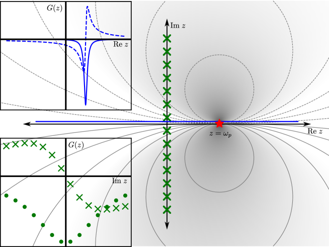
Figure 1: Simple one-pole Green’s function $G(z)=1/(z-\omega_{p})$ on the plane of complex frequencies $z$. The background density/contours show only $|\mathrm{Im}\,G(z)|$. The pole location $\omega_{p}$ is marked by a red asterisk. The inset in the upper left shows the retarded Green’s function (evaluated along the blue line on the complex plane), where the full line is the imaginary part and the dashed line is the real part. Clearly, the imaginary part of the retarded Green’s function has a peak at $\omega=\omega_{p}$. The inset in the lower left shows the Matsubara Green’s function (evaluated at the green crosses on the complex plane). Its real and imaginary part are drawn by dots and crosses, respectively.

By applying the Sokhotski-Plemelj theorem (often called Weierstrass formula)

$$\mathrm{lim}_{\epsilon\rightarrow 0^{+}}\int_{-\infty}^{\infty}\!\!dx\,\frac{f(x)}{x+i\epsilon}=-i\pi f(0)+\mathcal{P}\int_{-\infty}^{\infty}\!\!dx\,\frac{f(x)}{x}$$ (6)

we obtain the important relation

$$A(\omega)=-\frac{1}{\pi}\mathrm{Im}G_{R}(\omega)=-\frac{1}{\pi}\mathrm{Im}G(\omega+i0^{+}).$$ (7)

3 Padé interpolation

In Section 2 we have seen that the Matsubara Green’s function is connected to the spectral density through the integral relation Eq. 5. Since the spectral density contains valuable information, it is of interest to extract the spectral density from the Matsubara Green’s function.

If the Green’s function is given analytically, one may just substitute $i\omega_{n}$ by $\omega+i0^{+}$. Considering that in most calculations the Green’s function is evaluated only numerically, a different approach is required.

A logical next step is to approximate the numerical values of the Green’s function by an analytical function, which can be evaluated on the real axis through substitution as above. This is realized in the technique of Padé approximants (Press et al., 2007), where a given set of data points is interpolated by a rational function. An efficient algorithm, designed for Green’s functions, was put forward already by Vidberg and Serene (1977). Although frequently called a fit, the Padé approximation is thus actually an interpolation of given data.

Vidberg and Serene (1977) show that using Padé approximants for analytic continuation works remarkably well. The authors however also discuss a major drawback of the method. Namely, it is by no means clear a priori, which Matsubara frequencies should be selected for constructing the interpolation. Instead they propose to compare several Padé approximants, where different sets of Matsubara frequencies are used.

Another problem in the construction of Padé approximants arises, when the data points on the imaginary axis are subject to stochastic uncertainty or noise. It is then impossible to still interpolate these points by a rational function without poles in the upper half-plane. However, noise has the potential to wreak havoc on the interpolation.

We illustrate this behavior in Fig. 2 by taking a simple test function with four poles. We evaluate it on a set of Matsubara frequencies and generate four test data sets with additional noise by adding random numbers from a normal distribution with four different standard deviations on different orders of magnitude. The Padé approximant constructed from the exact data (blue symbols) perfectly reproduces the original function, its poles coincide with the true poles (black boxes) of the analytic function. Adding noise of magnitude 10^-9 (orange symbols) just slightly shifts some of the poles, leaving the resulting spectral function practically unchanged. Noise of magnitude 10^-6 (green symbols) already has a much more drastic effect. Pairs of almost canceling poles and zeros appear on the upper half plane, which is necessary for interpolation of the noisy test data. Further increasing the standard deviation of the noise to 10^-3 (red symbols), a value that is by no means uncommon in actual numerical calculations, increases the number of pole-zero pairs and the spectral function is already somewhat deteriorated.

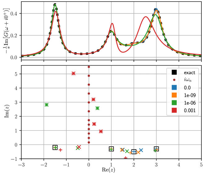
Figure 2: Padé approximation for a test function with four poles (black squares). The Matsubara frequencies used to construct the approximant are marked by red dots. Reconstructed poles and zeros are marked by $+$ and $\times$ symbols, respectively, with the color coding the noise level, see legend.

4 Probabilistic approach - Maximum Entropy

4.1 Formulation of the analytic continuation problem

Commonly employed are quantum Monte Carlo simulations, where the results intrinsically contain some uncertainty. Although we have shown above that the Padé approximation can yield good results even in the case of noisy data, it is difficult to assess its quality in real-world cases, where the exact solution is unknown. The interpolation treats data with random noise as if they were exact. Thus, the deviation of the spectral function from the true underlying spectral function has an element of arbitrariness.

For this reason, most methods for analytic continuation do not try to construct an exactly interpolating analytic function. Instead, one tries to answer the following question: Assume that $N$ normal-distributed data $G_{n}$ have been measured with corresponding uncertainty $\sigma_{n}$. Given a linear relation like Eq. 5 between the spectral function $A(\omega)$ and $G_{n}$,

$$G_{n}=\int_{-\infty}^{\infty}\!\!d\omega\,K(i\omega_{n},\omega)\,A(\omega)\hskip 20.00003pt\text{or in operator notation}\hskip 20.00003ptG=KA,$$ (8)

what is the most probable spectral function $A(\omega)$ that fits the data? One can immediately write down the probability for measuring $G$ if the spectral function is $A(\omega)$:

$$\mathrm{Pr}[G|A]=\frac{(2\pi)^{-N/2}}{\prod_{i}\sigma_{i}}\mathrm{exp}\big{[}-\sum_{i}\frac{(G_{i}-KA)^{2}}{2\sigma_{i}^{2}}\big{]}$$ (9)

The maximum likelihood method [cf., e.g., Press et al. (2007)] is based on the assumption that this is numerically equivalent to the probability of $A$ being the true spectral function, after $G$ has been measured (assuming we have no a priori information about $A$):

$$\mathrm{Pr}[A|G]=\mathrm{Pr}[G|A].$$ (10)

Then, the most probable spectral function is the one that maximizes the exponent of Eq. 9, or in other words, minimizes the merit function $\chi^{2}$

$$\chi^{2}[A]=\sum_{n=1}^{N}\frac{[G_{n}-\int\!\!d\omega\,K(i\nu_{n},\omega)\,A(\omega)]^{2}}{\sigma_{n}^{2}}.$$ (11)

This is a general least squares problem (Press et al., 2007). Let us for further analysis discretize the integral,

$$\int\!\!d\omega\,K(i\nu_{n},\omega)\,A(\omega)\approx\sum_{k}K(i\nu_{n},\omega_{k})A(\omega_{k})\Delta\omega_{k}.$$ (12)

Only for the sake of demonstration, assume that the measurement uncertainty $\sigma_{n}$ is constant for all $n$ and the discretization of $\omega$ is uniform, $\Delta\omega_{k}=\Delta\omega$. In this case the least squares problem is reduced to the following set of linear equations:

$$0=G_{n}-\sum_{k}K_{nk}A_{k}\Delta\omega.$$ (13)

Hence, the kernel determines the “hardness” of the problem, and it is indicated to have a closer look at its properties.

4.2 Properties of the kernel

The kernel that relates spectral functions to Green’s functions in Matsubara frequencies is

$$K(i\nu_{n},\omega)=\frac{1}{i\nu_{n}-\omega}.$$ (14)

Here, $\omega$ is a frequency on the real axis and $i\nu_{n}$ are (fermionic or bosonic) Matsubara frequencies. The properties of the kernel are best understood by first discretizing the real-frequency axis, such that the kernel becomes a matrix $K_{jk}=K(i\nu_{j},\omega_{k})$. It is however not a quadratic matrix, since the number of real frequencies has to be large enough to resolve all features of the spectral function, whereas the number of Matsubara frequencies only has to be large enough to reach the asymptotic region. These criteria are mutually independent and thus it would not be justified to choose the kernel to be a quadratic matrix. Numerical necessity also often restricts the number of Matsubara frequencies.

A singular-value decomposition can be readily performed also for general non-quadratic matrices:

$$K_{jk}=\sum_{m}U_{jm}\xi_{m}V_{km},$$ (15)

where $U$ and $V$ are column-orthogonal matrices and $\xi$ is the vector of singular values. In Fig. 3 the imaginary part of the matrix $V^{T}$ is shown, together with the singular values. The columns of $V$ can be understood as basis functions for the spectral function (Shinaoka et al., 2017). The contribution of the $m$-th component of the spectral function in this basis to the Matsubara data is then weighted by the $m$-th singular value. Since only few singular values are of significant size, the problem of minimizing $\chi^{2}$ in Eq. 11 is ill-conditioned and there is a large space of degenerate solutions.

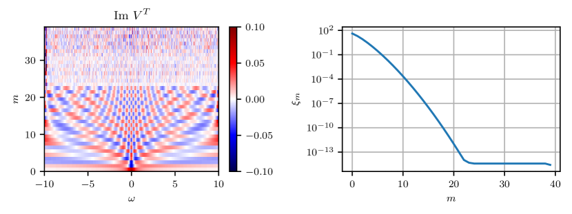
Figure 3: Singular-value decomposition of the kernel for the analytic continuation [Eq. 15]. Left panel: matrix of right singular vectors $V_{m}(\omega)$ ($m$: number of the singular value). Right panel: log-plot of the singular values $\xi_{m}$.

4.3 Regularization term or prior probability

If there are many completely different solutions to the problem, this may mean that we do not have enough information to actually solve the problem. It may however also mean that we do not use all our knowledge about the problem in the right way. Our inference has to make use of all available information, and this can be done by means of Bayes’ theorem

$$\mathrm{Pr}[A|G]=\frac{\mathrm{Pr}[A]\;\mathrm{Pr}[G|A]}{\mathrm{Pr}[G]},$$ (16)

where we want to find the spectral function $A$ (hypothesis) that maximizes the conditional or posterior probability $\mathrm{Pr}[A|G]$ of the hypothesis being true if data $G$ have been measured. The likelihood function $\mathrm{Pr}[G|A]$ has already been defined in Eq. 9. Additionally, with $\mathrm{Pr}[A]$ and $\mathrm{Pr}[G]$ we now have the prior probabilities of the hypothesis and the data, respectively. Eq. 16 is much richer compared to Eq. 10 and there is hope that with Bayesian statistics we get better results than with the maximum likelihood method. However, we first have to model the prior probability of a spectral function, $\mathrm{Pr}[A]$. This modeling is not univocal (Press et al., 2007), but a highly successful and state of the art choice of the entropic prior is

$$\mathrm{Pr}[A]\propto e^{\alpha S[A]}$$ (17)

with the entropy

$$S[A]=\int d\omega\left[A(\omega)-D(\omega)-A(\omega)\,\mathrm{log}\frac{A(\omega)}{D(\omega)}\right]$$ (18)

relative to a default model $D(\omega)$. This leads to the maximum entropy method (MaxEnt). The concept of entropy was introduced into information theory by Shannon (1948), and Jaynes (1957) established the principle of maximum entropy as “a method of reasoning” in statistical mechanics. Very successfully the maximum entropy method was employed for deconvolution of optical data (Frieden, 1972; Gull and Daniell, 1978). After further developments and applications to image processing (Gull and Skilling, 1984), it was also applied to the analytical continuation problem (Silver et al., 1990b, a; Jarrell and Gubernatis, 1996).

Combining Eq. 16 with Eq. 9, Eq. 17, and Eq. 18, we have to maximize the probability

$$\mathrm{Pr}[A|G]=\frac{1}{\mathrm{Pr}[G]}e^{-Q_{\alpha}[A]},$$ (19)

where

$$Q_{\alpha}[A]=\frac{1}{2}\chi^{2}[A]-\alpha S[A]$$ (20)

with a yet unspecified scaling hyperparameter $\alpha>0$. The prior probability of the data, $\mathrm{Pr}[G]$, also referred to as evidence, is fixed, since we are working with one measured data set. Therefore it does not depend on the spectral function and in our considerations can be absorbed in the normalization of $\mathrm{Pr}[A|G]$.

Instead of the least-squares problem of Eq. 11 we now face the minimization of the functional $Q_{\alpha}[A]$. The entropy, which was introduced as the prior probability of the spectral function, now serves as a regularization term to the ill-conditioned least-squares problem. This becomes apparent by looking at the Hessian matrix of $Q$ with respect to $A$:

$$\frac{\partial^{2}Q_{\alpha}}{\partial A_{l}\,\partial A_{m}}=\sum_{n}\frac{K_{nl}\Delta\omega_{l}\,K_{nm}\Delta\omega_{m}}{\sigma_{n}^{2}}+\alpha\delta_{lm}\frac{\Delta\omega_{l}}{A_{l}},$$ (21)

which is here computed by choosing a discretization of the real-frequency axis and deriving by the value of the spectral function at these discrete points. The first term of Eq. 21 contains a product $K^{T}K$, thus its conditioning is even worse than that of $K$: most of its eigenvalues are practically zero. However, the second term of Eq. 21 adds a positive diagonal matrix, scaled by $\alpha$. This has the effect of increasing the eigenvalues, i. e. the curvature of $Q$ at its minimum, and thus makes it easier to actually locate the minimum.

Let us note that, instead of the entropy, one may also choose a different regularization term. Otsuki et al. (2017) introduced the so-called sparse modeling technique, where solutions are prioritized if they are sparse in the singular space of the kernel. An implicit regularization effect can be achieved in stochastic sampling methods (Sandvik, 1998; Mishchenko et al., 2000; Nordström et al., 2016; Ghanem and Koch, 2020).

5 Technical aspects of the Maximum Entropy method

5.1 Choice of the hyperparameter $\alpha$

Having seen that the functional $Q_{\alpha}[A]$ can be minimized for $\alpha>0$, we now have to determine how to actually choose a good value of $\alpha$. The importance of this choice is illustrated in Fig. 4. We choose the asymmetric two-peak spectrum that is shown as a black curve in the right panel. By Eq. 14 it is transformed to Matsubara frequencies, and noise with an amplitude of 10^-4 is added. Assuming a flat default model, we calculate the spectral function $A(\omega)$ that minimizes Eq. 20 for a large range of different values of $\alpha$.

The influence of $\alpha$ is shown as a density plot in the top left panel of Fig. 4. At very high values of $\alpha$, we recover the constant default model, no influence of the data can be noticed. As $\alpha$ is decreased, the spectral weight concentrates in the middle, then we observe the formation of two distinct peaks. At small values of $\alpha$, the peaks split and in the end we get six very sharp peaks instead of two broad ones. The number and positions of such peaks is largely determined by the noise of the data. In our test case, we could generate the noise with a different random seed, which would lead to a seemingly completely different spectrum in the low-$\alpha$ limit.

Since apparently the result of the analytic continuation is to a large extent controlled by $\alpha$, it is extremely important to choose it in a reasonable and automatizable way. Various approaches have been proposed in order to tackle this problem.

In so-called historic MaxEnt, $\alpha$ was chosen in a way that the $\chi^{2}$-deviation (Eq. 11) is approximately equal to the number of data points on the imaginary axis (Gull, 1989). It was however found to under-fit the data and both Gull (1989) and Skilling (1989) argue that it is somewhat ad hoc.

The classic MaxEnt extends the Bayesian inference scheme to $\alpha$ and $D$ (Skilling, 1989; Jarrell and Gubernatis, 1996):

$$\mathrm{Pr}[A,\alpha|G,D]\propto\mathrm{Pr}[A|G,D,\alpha]\mathrm{Pr}[\alpha]\propto\frac{e^{-Q_{\alpha}[A]}}{\alpha},$$ (22)

where the scale invariant Jeffreys’ prior $1/\alpha$ (Jeffreys, 1939) was used for the prior probability of $\alpha$. Subsequently, the dependence on the spectral function in Eq. 22 is integrated out and one obtains an explicit form for $\mathrm{Pr}[\alpha|G,D]$. In the bottom left panel of Fig. 4 the logarithm of the posterior probability $\mathrm{Pr}[\alpha|G,D]$ is shown as an orange curve. Classic MaxEnt takes the spectral function at the most probable value of $\alpha$ to be the best solution to the problem. This value is usually obtained by setting $\partial\mathrm{Pr}[\alpha|G,D]/\partial\alpha=0$, which can be analytically transformed to an equation $N_{g}=-2\alpha S$ after a few approximations. $N_{g}$ is called the “number of good measurements”, for its definition we refer to Jarrell and Gubernatis (1996). In the bottom left panel of Fig. 4 we plot $-N_{g}/2\alpha S$ as a blue line; its intersection with 1 is the classic MaxEnt solution, marked by a blue vertical line. The corresponding spectrum is shown in the right panel.

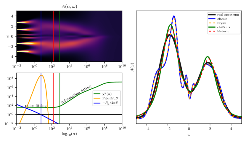
Figure 4: Methods for determining $\alpha$. A model spectrum (black curve in the right panel) is transformed to Matsubara frequencies and normal-distributed noise with amplitude $10^{-4}$ is added. Upper left panel: spectral function $A$ (color code) obtained through the minimization of the MaxEnt functional $Q_{\alpha}$ for a range of values of $\alpha$. Lower left panel: illustration of the four different methods of determining the optimal value of $\alpha$. Here the red and blue vertical lines mark historic and classic MaxEnt, respectively (cf. colors in the legend of the right panel). The value of $\alpha$ obtained by the “chi2kink” method is marked by a green vertical line. Note that Bryan’s method can not be highlighted in such a way since it is a weighted average over a range of $\alpha$ (in this case the probability that serves as a weight is drawn in orange.) Lower right panel: Spectral functions obtained by the four different methods compared to the real (initial) spectrum.

Closely related is Bryan’s method (Bryan, 1990), where one takes the average over all values of $\alpha$, weighted by the probability:

$$A(\omega)=\int d\alpha\,A(\alpha,\omega)\,\mathrm{Pr}[\alpha|G,D]$$ (23)

The results are usually very close to classic MaxEnt, since the probability of $\alpha$ is sharply peaked, see the blue and orange dashed lines in Fig. 4. As one can clearly see, the solutions of classic and Bryan’s MaxEnt may lead to unphysical extra peaks — a drawback already noticed by Gull (1989).

However, there is yet another approach to the decision of the best $\alpha$. It is based on the so-called L-curve criterion (Lawson and Hanson, 1974, 1995). In the context of MaxEnt, it was to our knowledge first proposed and explained by Bergeron and Tremblay (2016) and in the following also applied by Kraberger et al. (2017). It is somewhat more heuristic than classic or Bryan’s MaxEnt in that it relies only on the behavior of $\chi^{2}$ (like historic MaxEnt). For apprehending this approach, we plot $\chi^{2}$ as a green curve in the lower left panel of Fig. 4. In the limit of $\alpha\rightarrow\infty$ it goes to a constant high value, and for $\alpha\rightarrow 0$ another constant of lower value is approached. Following the reasoning of Bergeron and Tremblay (2016), there is a clear interpretation for this behavior. In the high-$\alpha$ limit, the (large) $\chi^{2}$-deviation has negligible weight, such that the default model $D$ minimizes $Q_{\alpha}[A]$. What we see is thus $\chi^{2}[A=D]$. On the other hand, in the low-$\alpha$ limit, the contribution of the entropy is reduced to enforcing positivity of the spectrum; and $\chi^{2}$ slowly approaches its global minimum. The low-$\alpha$ region, where $\chi^{2}$ is relatively flat, and the subsequent region with steep increase of $\chi^{2}$, are coined noise-fitting and information-fitting regions (Bergeron and Tremblay, 2016). The optimal value of $\alpha$ is situated in the transition region between information fitting and noise fitting, where $\mathrm{log}\chi^{2}(\mathrm{log}\alpha)$ has a kink. We therefore call this method to determine $\alpha$ “chi2kink”. This optimal $\alpha$ is indicated by a maximum in the curvature $\chi^{\prime\prime}(\alpha)$ (Bergeron and Tremblay, 2016; Kraberger et al., 2017). A more numerically stable and flexible approach is to fit a function

$$\phi(x;a,b,c,d)=a+\frac{b}{1+e^{-d(x-c)}}$$ (24)

to several values of $\mathrm{log}_{10}\chi^{2}(\mathrm{log}_{10}\alpha)$. The curvature of $\phi$ in Eq. 24 is maximal at $x=c-\mathrm{ln}(2+\sqrt{3})/d\approx c-1.317/d$. Since this usually leads to strong underfitting, we suggest to use a more general $x=c-f/d$ or $\alpha=10^{c-f/d}$, with preferred values of $f\in[2,2.5]$. In Fig. 4 the value corresponding to $f=2$ is marked by green vertical lines.

In summary, historic MaxEnt seems to underfit only with respect to classic MaxEnt, since the latter tends to grave overfitting. Bergeron and Tremblay (2016) note that the formula for the posterior probability of $\alpha$ is an approximation that works well only when a good default model is used.

In order to get good results with classic MaxEnt, it has therefore become common practice to increase the standard deviation $\sigma_{n}$ by a manually chosen factor to shift the peak in the probability to a larger value of $\alpha$. Since the rescaling factor is not known a priori (although a dependence on the actual noise amplitude is noticed), this procedure introduces an additional degree of arbitrariness.

Determining the optimal $\alpha$ as the point where noise-fitting starts and information fitting ends (“chi2kink”) leads to considerably larger values of $\alpha$, even with respect to historic MaxEnt. Despite the drawback of being less “Bayesian”, it does not rely on additional approximations and the noise amplitude of the data has to be known only up to a constant prefactor. The only remaining source of arbitrariness is the parameter $f$ mentioned above, which controls the actual value of $\alpha$ to be accepted. It is however restricted to a rather narrow range, whereas the error rescaling factor in classic MaxEnt can vary by several orders of magnitude.

At least in the present context of analytic continuation, we are therefore convinced that the best method of determining $\alpha$ is extracting it as the border between noise- and information-fitting.

5.2 Elimination of unphysical features: Preblur

Even though we are now able to find the “best” value of $\alpha$, the spectrum corresponding to it may show some undesirable artifacts. In the right panel of Fig. 4 we can see that all solutions have an enlarged curvature around $\omega=0$ and side peaks emerge upon lowering $\alpha$. An analogous tendency was observed already in the original application of MaxEnt in image processing, where it manifested itself in huge peaks in the intensity distribution. In order to address this problem, Skilling (1991) showed that the entropy does not need to be evaluated from the spectral function directly, but from a “hidden” function $h(\omega)$ that is related to the spectral function in a linear way

$$A=\Omega h.$$ (25)

In standard MaxEnt, $\Omega$ is just unity. Although initially requiring $\Omega$ to be an orthogonal matrix, Skilling (1991) subsequently assumed a Gaussian convolution $A=g_{b}\!\ast\!h$ with great success and named the technique “preblur”. In the latter case, $\Omega$ is a matrix that contains a Gaussian function $g_{b}(\omega)=\mathrm{exp}[-\omega^{2}/2b^{2}]/\sqrt{2\pi}b$ in each row, i.e. $\Omega_{ij}=g_{b}(\omega_{i}\!-\!\omega^{\prime}_{j})$. In the context of analytic continuation, preblur was introduced by Kraberger et al. (2017), although already Sandvik (1998) uses a somewhat similar smoothing algorithm.

The functional of Eq. 20, which we have to minimize, thus becomes

$$Q_{\alpha b}[h]=\frac{1}{2}\chi^{2}[g_{b}\!\ast\!h]-\alpha S[h].$$ (26)

There we now have, after $\alpha$, a second hyperparameter $b$ that controls the width of the Gaussian $g$.

Let us now have a closer look at the $\chi^{2}$-term of Eq. 26. It sums up the difference of the fit “$KA$” to the data $G$. Explicitly the fit function is now

$$KA \equiv\int_{-\infty}^{\infty}d\omega\,K(i\nu_{n},\omega)\,A(\omega)$$

$$=\int_{-\infty}^{\infty}d\omega\,K(i\nu_{n},\omega)\,\int_{-\infty}^{\infty}d\omega^{\prime}\,g_{b}(\omega-\omega^{\prime})\,h(\omega^{\prime})$$

$$=\int_{-\infty}^{\infty}d\omega\Big{[}\int_{-\infty}^{\infty}d\omega^{\prime}\,K(i\nu_{n},\omega^{\prime})\,g_{b}(\omega-\omega^{\prime})\Big{]}h(\omega)$$

$$\equiv\tilde{K}h.$$ (27)

This means that the hidden spectral function is related to the Matsubara Green’s function in a similar way as the spectral function, the only difference being a “blurred” kernel $\tilde{K}$. Therefore, preblur is realized by minimizing the functional $Q$ with a slightly modified kernel, which then yields the hidden spectral function $h$. The spectral function $A$ itself is subsequently obtained by the convolution of $h$ with the same Gaussian $g_{b}(\omega)$ as above.

Although the minimization of $Q$ itself does not become more difficult by introducing preblur, we now face the problem that the blur width $b$ is not known a priori, similar as the entropy-scaling parameter $\alpha$. However, knowing that we can determine a good value for $\alpha$ by analyzing $\chi^{2}(\alpha)$, it is now worth to analyze the $\chi^{2}$-deviation as a function of both $\alpha$ and $b$. This is done in the upper left panel of Fig. 5. Over a large range of $b$, $\chi^{2}$ depends only on $\alpha$. Only after a sharp border (at $b\approx 1$ in our example) the $\chi^{2}$-deviation increases steeply with $b$, which can be seen best in the lower left panel of Fig. 5. In other words, increasing $b$ up to a certain value does not change the quality of the fit (but potentially the result.) Only afterwards it is suddenly impossible to get a good fit. A heuristic explanation of this is that convolving the kernel with a Gaussian permits only peaks with a minimal width of $2b$ in the spectrum. Once this exceeds the “real” width of one of the peaks in the spectrum, a fit becomes impossible. This observation is corroborated by the fact that we find the maximal permissive $b$ to be close to $1$ in Fig. 5, and the actual spectrum (black curve) consists of two Gaussians with standard deviation 1.

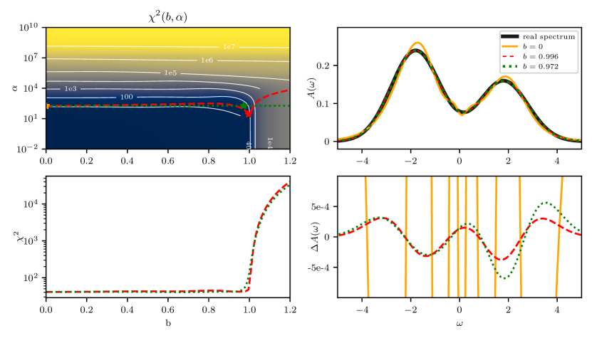
Figure 5: Analyzing the preblur-parameter $b$. Upper left panel: $\chi^{2}$-deviation (color code and isolines) of the MaxEnt fit as a function of the hyperparameters $b$ and $\alpha$. The red dashed line marks the optimal $\alpha$ at each $b$, the green dotted line shows the optimal $\alpha$ at $b=0$ for comparison. Lower left panel: $\chi^{2}$ along the red dashed and green dotted lines in the upper left panel. Upper right panel: The true spectral function (black), and its MaxEnt reconstructions at the points marked by orange, red and green asterisks in the upper left panel, drawn in the respective colors. The lower right panel shows the differences of these reconstructions to the true spectrum. The orange $\Delta A(\omega)$ (corresponding to $b=0$) is as large as $10^{-2}$.

The observations made in the upper left panel of Fig. 5 can be used to propose the following algorithm for the determination of the hyperparameters: Determine the optimal $\alpha$ for different values of $b$, starting from 0 and increasing. Accept the last value of $b$ where $\chi^{2}$ at the optimal $\alpha$ is smaller than, e. g., 1.5 times $\chi^{2}$ at the optimal $\alpha$ for $b=0$. The optimal values of $\alpha$ are marked as a red dashed line in the upper left panel of Fig. 5, and the thus determined $(\alpha,b)$ is marked by a red asterisk. Since the optimal values of $\alpha$ hardly change in the reasonable range for $b$, one may also use a simplified algorithm: Determine the optimal $\alpha$ for $b=0$, then increase $b$, keeping always the same $\alpha$. If $\chi^{2}$ exceeds, e. g., 1.5 times its value at $b=0$, accept the last value of $b$ before this as the best value. The corresponding $(\alpha,b)$ is marked in Fig. 5 by a green asterisk.

As we can see in the upper right panel, the corresponding red and green curves obtained by analytic continuation with these two $(\alpha,b)$ are practically indistinguishable. In the lower right panel, the differences of these reconstructed spectra are plotted and show that the deviation from the actual result is now satisfactorily small.

Let us note in passing that the above described unphysical wiggles around $\omega=0$ are most prominent in spectral functions similar to our example case. In cases where the spectral function shows a gap or a peak at $\omega=0$, preblur is usually not required.

5.3 MaxEnt for offdiagonal elements

The considerations above were done for positive definite spectral functions with a finite norm, typically one: $\int d\omega A(\omega)=1>0$. This property is fulfilled by diagonal elements of correlation functions. In some cases it is however necessary to do an analytic continuation of offdiagonal elements, which have zero norm $\int d\omega A(\omega)=0$, as a direct consequence of the fermionic anticommutation relation. A vanishing norm is not consistent with a positive definite function, thus the spectral function cannot have a definite sign for offdiagonal elements. Clearly the definition of the entropy, Eq. 18, has to be adapted to this new circumstance (Kraberger et al., 2017). At this point, let us mention that the kernel $K(i\omega_{n},\omega)$ is the same for diagonal and offdiagonal elements.

Let us, for offdiagonal components, write the spectrum as

$$A(\omega)=A^{+}(\omega)-A^{-}(\omega),$$ (28)

where both $A^{+}$ and $A^{-}$ are positive definite and have the same norm. Then we can write the entropy as

$$S[A^{+},A^{-}]=\int d\omega\Big{[} A^{+}(\omega)-D(\omega)-A^{+}(\omega)\,\mathrm{log}\frac{A^{+}(\omega)}{D(\omega)}$$

$$+ A^{-}(\omega)-D(\omega)-A^{-}(\omega)\,\mathrm{log}\frac{A^{-}(\omega)}{D(\omega)}\Big{]}$$ (29)

Instead of treating $A^{+}$, $A^{-}$ and $A$ as completely independent, we can use Eq. 28 to eliminate $A^{-}$ and write

$$Q_{\alpha}[A,A^{+}]=\frac{1}{2}\chi^{2}[A]-\alpha S[A,A^{+}].$$ (30)

Since we are searching for a minimum of $Q$ with respect to both $A$ and $A^{+}$, we can use

$$\frac{\partial Q_{\alpha}[A,A^{+}]}{\partial A^{+}}=-\alpha\frac{\partial S[A,A^{+}]}{\partial A^{+}}=0$$ (31)

to eliminate also $A^{+}$. Substituting $A^{-}=A-A^{+}$ in Section 5.3 and taking the derivative, $A^{+}$ and $A^{-}$ can be expressed by $A$ as

$$A^{\pm}[A]=\frac{\sqrt{A^{2}+4D^{2}}\pm A}{2}.$$ (32)

Inserting this back in Section 5.3, we arrive at the so-called positive-negative entropy

$$S[A]=\int d\omega\,A(\omega)\,\mathrm{log}\frac{A^{+}[A](\omega)}{D(\omega)}.$$ (33)

As a reasonable choice for the default model, Kraberger et al. (2017) propose to include the diagonal elements of the spectrum in the following way:

$$D_{ll^{\prime}}=\sqrt{A_{ll}A_{l^{\prime}l^{\prime}}}+\varepsilon.$$ (34)

In our implementation, it is not necessary to add a small number $\varepsilon$.

Also methods that continue matrix-valued Green’s functions as a whole, and not component-wise, have been developed (Kraberger et al., 2017; Sim and Han, 2018).

6 Python package for analytic continuation: ana_cont

In the previous sections we have presented two methods for analytic continuation, the Padé approximation and the maximum entropy method. Although both of them are well-established and have been implemented before [e.g. by Bergeron and Tremblay (2016), Levy et al. (2017), Kraberger et al. (2017)], we here introduce yet another code for analytic continuation. In contrast to other implementations, it is a Python package. The advantage of this approach is increased maintainability. There are too many ways of doing analytic continuation to encode all of them into a few command line arguments. The ana_cont package is available open source at https://github.com/josefkaufmann/ana_cont.

6.1 Package structure

The central class of ana_cont is AnalyticContinuationProblem, which holds problem-specific information: real-frequency grid, imaginary frequency or time grid, data on imaginary axis, inverse temperature, and type of the kernel, see Table 1. It has a method solve, which takes several keyword arguments. The most important one is method. Currently, only two methods, pade and maxent_svd are implemented. Calling solve creates an instance of a solver object. In case of method=’maxent_svd’, the class MaxentSolverSVD is instantiated. The class contains all necessary functions to solve the analytic continuation problem defined before. Possible keyword arguments are listed in Table 2.

keyword	value
im_axis	numpy array, shape $(N_{\text{mats}},)$
re_axis	numpy array, shape $(N_{\text{real}},)$
im_data	numpy array, shape $(N_{\text{mats}},)$, float or complex
kernel_mode	one of ’freq_fermionic’, ’freq_bosonic’, ’time_fermionic’, ’time_bosonic’
beta	float (only required for “time” kernels)

Table 1: Keyword arguments for initializing the AnalyticContinuationProblem.

keyword	value
method	’maxent_svd’
optimizer	one of ’scipy_lm’, ’newton’
alpha_determination	one of ’historic’, ’classic’, ’bryan’, ’chi2kink’
model	default model: numpy array, shape $(N_{\text{real}},)$
stdev	error bars: numpy array, shape $(N_{\text{mats}},)$
covar	covariance matrix: numpy array, shape $(N_{\text{mats}},N_{\text{mats}},)$
alpha_start	float, default $10^{9}$
alpha_end	float, default $10^{-3}$
alpha_div	float, default $10$
fit_position	float, default 2.5
interactive	boolean, default False
preblur	boolean, default False
blur_width	float

Table 2: Possible keyword arguments for AnalyticContinuationProblem.solve() when using MaxEnt.

The kernel for the continuation problem at hand is provided by the class Kernel. It handles real-frequency discretization of the kernel, preblur, and rotation to the eigenbasis of the covariance matrix if provided.

Furthermore there is a class GreensFunction, whose main purpose is to construct a full complex-valued Green’s function out of a given spectrum, by applying the Kramers-Kronig relation Eq. 5.

We want to stress that this package does not contain a “main program” that can access all features by just specifying some parameters. While this may sound rather discouraging, we believe that in fact this reduces the required amount of work both for the user and for the maintainer. On the user-side, a working script can be composed of as few as 10 lines of Python code; example scripts can be found in the GitHub repository. There is full freedom in which way to provide the imaginary-axis data: They can be read from a favorite file format, or calculated on-the-fly. Computed real-axis data can be plotted or further processed without the detour of file-IO. Thus the present analytic continuation code can be easily embedded in complex postprocessing procedures. Also for the developers this principle is a large gain, since they do not have to take care of a sophisticated user interface and flow control. Since knowledge and experience of analytic continuation are absolutely necessary to use any analytic continuation program, we do not see a principal downside to this approach.

However, for the casual user, we have cast in scripts a few standard procedures for analytic continuation with a graphical user interface (GUI). Thus, most of the standard analytic continuations of bosonic and fermionic Green’s functions by MaxEnt and Padé can be done even without knowledge of Python. Tutorials for the GUI can be found in the wiki of our repository on GitHub: https://github.com/josefkaufmann/ana_cont/wiki

6.2 Numerics

Analytic continuation is, compared to large quantum Monte Carlo simulations or Bethe-Salpeter equation inversions, a numerically rather inexpensive task. Therefore the performance of the code does not have to be the main goal. The ana_cont package is written entirely in Python, partly trading performance for flexibility and readability, while still keeping the possibility of later optimization. Nevertheless several actions have been taken in order to make the code reasonably fast – a typical MaxEnt analytic continuation takes just O(1) seconds on an average desktop computer.

6.2.1 Frequency-space discretization.

For a numerical treatment it is necessary to discretize the real-frequency axis: $\omega\rightarrow\omega_{i}$. For an arbitrary function $F(\omega)$ we then define $F_{i}\equiv F(\omega_{i})$. Integrals over frequency space are converted to sums by $\int d\omega F(\omega)\approx\sum_{i}F_{i}\Delta_{i}$, where $\Delta_{i}$ is the width of the frequency interval centered at $\omega_{i}$.

6.2.2 Singular value decomposition.

One of the most important steps of MaxEnt is the minimization of the functional $Q_{\alpha}[A]$ in the space of spectral functions. If the real-frequency axis is discretized into, say, 1000 intervals, the space of solutions has 1000 dimensions. This is too large for a deterministic solver, and a Monte Carlo method is needed (Sandvik, 1998). However, Jarrell and Gubernatis (1996) perform a singular value decomposition of the kernel and thereby achieve a large reduction of dimensions, e. g. from 1000 to 20 in typical cases. The optimization problem can then be solved by deterministic methods like Newton root finding or the Levenberg-Marquart algorithm. The MaxentSolverSVD follows the strategy of singular value decomposition of the kernel, as defined in Eq. 15. The vector $\xi$ of singular values is truncated such that only values larger than a certain threshold ($10^{-10}$ in our case) are kept. In the singular space the spectrum is parameterized through

$$A_{j}=D_{j}\mathrm{exp}\sum_{m}V_{jm}u_{m}$$ (35)

as proposed by Jarrell and Gubernatis (1996).

6.2.3 Minimization problem.

The above definitions are inserted into Eq. 20, and after a few intermediate steps the stationary condition $\partial Q_{\alpha}/\partial A_{m}=0$ leads to

$$f_{m}(u)\equiv\alpha u_{m}+\xi_{m}\sum_{k}E_{k}U_{km}\left(\sum_{l}K_{kl}A_{l}(u)\Delta_{l}-G_{k}\right)=0,$$ (36)

which has to be solved for $u_{m}$. Root finding algorithms work better, when the derivative of the root function is known analytically. Therefore, we take the derivative of $f$ with respect to $u$ to get the Jacobian $J$:

$$\frac{\partial f_{m}}{\partial u_{i}}\equiv J_{mi}=\alpha\delta_{mi}+\xi_{m}\sum_{k}U_{km}E_{k}\sum_{l}K_{kl}\Delta_{l}A_{l}(u)V_{li}$$ (37)

The expressions Eq. 36 and Eq. 37 can be put in a form that is more efficient for numerical evaluation by making the following definitions:

$$w_{l} \equiv \mathrm{exp}\left(\sum_{m}V_{lm}u_{m}\right)$$ (38a)

$$W_{ml} \equiv \sum_{km}E_{k}U_{km}\xi_{m}U_{kn}\xi_{n}V_{ln}\Delta_{l}D_{l}$$ (38b)

$$W_{mil} \equiv W_{ml}V_{li}$$ (38c)

$$B_{m} \equiv \sum_{k}U_{km}\xi_{m}E_{k}G_{k}$$ (38d)

Then we have

$$f_{m} = \alpha u_{m}+\sum_{l}W_{ml}w_{l}-B_{m}$$ (39a)

$$J_{mi} = \alpha\delta_{mi}+\sum_{l}W_{mil}w_{l},$$ (39b)

where the quantities $W_{ml}$, $W_{mil}$, and $B_{m}$ are precomputed in order to minimize the number of matrix multiplications during the optimization procedure. Please note that we do not use the Einstein summation convention. For the optimization, the Levenberg-Marquart implementation of scipy.optimize.root can be used by passing optimizer=’scipy_lm’ to the solver. However, we find simple Newton root finding to be much faster and numerically stable. This is activated by setting optimizer=’newton’.

6.2.4 Offdiagonal elements.

While the above formulas are used for diagonal elements of correlation functions, with only very small changes we arrive at a different form that can be used for offdiagonal elements. The singular-space parameterization becomes (Kraberger et al., 2017)

$$A_{j}=D_{j}\left[\mathrm{exp}\left(\sum_{m}V_{jm}u_{m}\right)-\mathrm{exp}\left(-\sum_{m}V_{jm}u_{m}\right)\right]=D_{j}\left(w_{j}-1/w_{j}\right)$$ (40)

and the minimization problem is set by

$$f_{m} = \alpha u_{m}+\sum_{l}W_{ml}(w_{l}-1/w_{l})-B_{m}$$ (41a)

$$J_{mi} = \alpha\delta_{mi}+\sum_{l}W_{mil}(w_{l}+1/w_{l}).$$ (41b)

6.2.5 Determination of optimal $\alpha$.

In Section 5.1 we have discussed various ways of determining a good value of the hyperparameter $\alpha$. All of these methods are implemented in ana_cont and can be used by setting the solver keyword alpha_determination to one of ’historic’, ’classic’, ’bryan’ or, as recommended, ’chi2kink’.

From the algorithmic point of view, all these methods have in common that the optimization is done for several values of $\alpha$, where one starts at a very high value of, e.g., $\alpha=10^{12}$. If alpha_determination=’chi2kink’, this can be adapted by setting the keyword alpha_start. One should use a value that leads to a solution very close to the default model. Subsequently $\alpha$ is decreased by a constant factor alpha_div in each step, which has the advantage that the solution of the previous step can be used as a starting point. After reaching the smallest value of $\alpha$ (alpha_end) the function of Eq. 24 is fitted and the parameter $f$ is specified by the keyword fit_position. One has to be especially careful about the choice of $\alpha$ when continuing offdiagonal elements of correlation functions. With a spectrum that is not positive definite, one has more degrees of freedom for noise fitting. Therefore in the double logarithmic plot of $\chi^{2}(\alpha)$ the noise fitting region may not any more be a plateau, but rather another, less steep linear slope. The optimal $\alpha$ has to be chosen at the point, where the slope changes.

6.2.6 Preblur

Maxent with preblur, as described in Section 5.2 is implemented in ana_cont. Preblur is activated by passing preblur=True to the solver, and specifying the parameter $b$ by blur_width=$b$. Our recommended workflow is to always first do an analytic continuation with $b\!=\!0$, and then increase it step-by-step. The final value $b^{\ast}$ should be large enough to eliminate spurious features in the spectrum, but still small enough so that the limit $\lim_{\alpha\rightarrow 0}\mathrm{log}\chi^{2}(\alpha)$ is not significantly increased with respect to $b=0$.

6.3 MaxEnt for susceptibilities

The analytic continuation of susceptibilities, i. e. bosonic Green’s functions, from the imaginary to the real axis is a frequently required task. In ana_cont it can be achieved by initializing the AnalyticContinuationProblem with kernel_mode=’freq_bosonic’. Like in the case of fermionic correlation functions, a relation that connects the values of the susceptibility on the real and imaginary axis is required. A susceptibility $\chi(\omega)$ is a response function, therefore causality implies that its imaginary part is anti-symmetric in frequencies, $\chi(\omega)=\chi^{\ast}(-\omega)$. Inserting this fact in the Kramers-Kronig relation

$$\mathrm{Re}\left[\chi(i\omega_{n})\right]=\frac{1}{\pi}\int_{-\infty}^{\infty}d\omega\,\frac{\mathrm{Im}\!\left[\chi(\omega)\right]}{\omega-i\omega_{n}}$$

yields

$$\mathrm{Re}\left[\chi(i\omega_{n})\right]=\frac{2}{\pi}\int_{0}^{\infty}d\omega\,\frac{\omega}{\omega^{2}+\omega_{n}^{2}}\,\mathrm{Im}\!\left[\chi(\omega)\right],$$

connecting the susceptibility at real frequencies with its values at the bosonic Matsubara frequencies $\omega_{n}$.
Since the factor $\omega/(\omega^{2}+\omega_{n}^{2})$ is divergent for $\omega=\omega_{n}=0$, it is common to introduce another function

$$S(\omega)\equiv\frac{2}{\pi}\frac{\mathrm{Im}\chi(\omega)}{\omega},$$ (42)

such that we can now write

$$\mathrm{Re}\!\left[\chi(i\omega_{n})\right]=\int_{0}^{\infty}d\omega\,K_{b}(\omega_{n},\omega)\,S(\omega)$$ (43)

with a kernel

$$K_{b}(\omega_{n},\omega)=\frac{\omega^{2}}{\omega_{n}^{2}+\omega^{2}}$$ (44)

that is well-defined for all values of $\omega$ and $\omega_{n}$. Correspondingly the result of the analytic continuation that is returned by the solver of ana_cont is $S(\omega)$.

Our ana_cont code has been used extensively for the analytic continuation of susceptibilities by Geffroy et al. (2019).

6.4 MaxEnt for self-energies

Besides one-particle Green’s functions and susceptibilities, it often is necessary to analytically continue self-energies from Matsubara to real frequencies. Self-energies essentially have the same analytic properties as one-particle Green’s functions (Luttinger, 1961). The difference is that the high-frequency limit is a non-zero constant $\Sigma_{0}$ (the so-called Hartree term), and the imaginary part decays like $\Sigma_{1}/(i\omega_{n})$ as opposed to $1/(i\omega_{n})$ in case of the Green’s function. $\Sigma_{0}$ and $\Sigma_{1}$ are called the zeroth and first moments of the self-energy and can be calculated from density matrices (Wang et al., 2011). The zeroth moment is frequently referred to as Hartree term. Note that $\omega_{n}$ are fermionic Matsubara frequencies here. In absence of particle-hole symmetry, the spectral representation is

$$\Sigma(i\omega_{n})=\Sigma_{0}+\Sigma_{1}\int_{-\infty}^{\infty}d\omega\,\frac{a(\omega)}{i\omega_{n}-\omega},$$ (45)

where we defined the spectrum $a$ of the self-energy as

$$a(\omega)\equiv-\frac{1}{\pi}\mathrm{Im}\frac{\Sigma(\omega)-\Sigma_{0}}{\Sigma_{1}}.$$ (46)

Thus, we can write the analytic continuation problem for the self-energy in a form very similar to Eq. 43:

$$\frac{\Sigma(i\omega_{n})-\Sigma_{0}}{\Sigma_{1}}=\int_{-\infty}^{\infty}d\omega\,K_{f}(\omega_{n},\omega)\,a(\omega)$$ (47)

with the fermionic kernel

$$K_{f}(\omega_{n},\omega)=\frac{1}{i\omega_{n}-\omega}.$$ (48)

We do not see any necessity for normalizing the self-energy by division through its first moment, but merely keep this notation for consistency with the literature. The solver of ana_cont then returns $a(\omega)$. From this we can construct the imaginary part of the retarded self-energy by inverting Eq. 47:

$$\mathrm{Im}\Sigma_{R}(\omega)=-\pi\Sigma_{1}a(\omega).$$ (49)

If one wants to use the retarded self-energy for the calculation of the retarded Green’s function, it is necessary to also obtain the real part of the retarded self-energy, which is given by the Kramers-Kronig relation Eq. 5. This is implemented in the kkt method of the GreensFunction class.

For a real-world case (SrVO₃) the procedure of analytic continuation of a self-energy, using MaxEnt and preblur, is illustrated in Fig. 6.

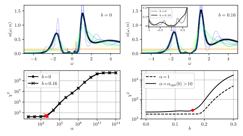
Figure 6: Analytic continuation of the DMFT self-energy of the V-$t_{2g}$ orbitals of SrVO₃ (Si et al., 2020), which was obtained with symmetric improved estimators for extra precision (Kaufmann et al., 2019). Upper row: Spectrum of the imaginary part of the self-energy spectrum $a(\omega)=-{\rm Im}\Sigma(\omega)/\pi$ for SrVO₃ without [left] and with [right] preblur. The figures show optimization results for several different values of $\alpha$. Red corresponds to $\alpha=10^{13}$, and as the color changes into blue, the value is lowered by a factor of $10$ in every step. The final result, at optimal $\alpha$, is drawn in black. Clearly, for the highest values of $\alpha$, we recover the constant default model. Lower row: Behavior of $\chi^{2}$ as a function of $\alpha$ [left] and $b$ [right] for the MaxEnt analytic continuation of SrVO₃. The values taken as optimal are highlighted in red.

7 Installation and Usage

7.1 Python 3

As a prerequisite for using the ana_cont package, you need to have Python 3 installed on your computer. This is possible via the official package repositories of most Linux distributions. After installing Python 3, it may also be necessary to install the Python package manager pip (again, from the official package repositories of your linux distribution). If necessary, you can use pip to install missing Python packages:

pip install --user <package_name>

Make sure that your Python 3 environment is actually activated and pip also refers to Python 3. In the Anaconda Python distribution all necessary packages are already included.

7.2 ana_cont

The program files for the ana_cont package can be downloaded from https://github.com/josefkaufmann/ana_cont in several ways. It is however recommended to use git:

git clone https://github.com/josefkaufmann/ana_cont.git

This will create a new directory ana_cont in your current working directory. Now change to this directory, cd ana_cont. There all the code files are located. If you plan to do analytic continuations by Padé interpolation, you have to compile the Padé core functions, which are written in Cython. The compilation is done by the setup script:

python setup.py build_ext --inplace

Now, in a Python script, you have to insert the path to the ana_cont package into the module search path and import the package:

import sys
sys.path.insert(0, ’/path/to/ana_cont/’)
import ana_cont.continuation as cont

Then the main classes, as described in Section 6, can be accessed as cont.AnalyticContinuationProblem and cont.GreensFunction. Before writing a custom script it is recommended to go through some of our learning resources on GitHub, e.g.

• doc/basics.ipynb,

• doc/tutorial/tutorial.ipynb,

• scripts/example_fermionic.py.

A tutorial related to the example case of Fig. 6 is doc/tutorial_svo.ipynb.

The Python scripts with GUIs, which are located in the scripts directory, are maxent.py (fermionic maxent), maxent_bosonic.py (bosonic maxent), and pade.py for the Padé method. All details about their execution and usage are documented in the wiki of our repository on GitHub at https://github.com/josefkaufmann/ana_cont/wiki. There we provide also tutorials with links for downloading files with test data.

8 Conclusion

We have given an introduction to analytic continuation by means of Padé interpolation and the maximum entropy method. These are implemented within our Python package ana_cont, which can be used with great flexibility for the analytic continuation of arbitrary bosonic and fermionic Green’s functions. Extensions to other analytic continuations outside the realm of quantum field theory are possible. Through casting our established workflows in applications with GUIs, we have also made MaxEnt and Padé analytic continuation accessible for non-experts. Long-term users, on the other hand, will value the flexibility and adaptibility of the Python package and adjust the provided scripts to their individual needs.

Acknowledgment

We are indepted to Patrik Gunacker, who gave the initial incentive to the development of this code, and to Andrey Katanin for sharing his knowledge and experience about the Padé method. Furthermore we thank Dominique Geffroy and Klaus Steiner, who motivated the implementation of many features by their extensive usage of the code. For diligent testing and numerous valuable comments we are grateful to Clemens Watzenböck, Jan Kuneš, Oleg Janson, and Markus Wallerberger. This work has been supported financially by the Austrian Science Fund (FWF) through projects P30819 and P32044.

References

- Abrikosov et al. (1975) Abrikosov, A.A., Dzyaloshinskii, I., Gorkov, L.P., 1975. Methods of quantum field theory in statistical physics. Dover, New York, NY. URL: https://cds.cern.ch/record/107441.
- Bergeron and Tremblay (2016) Bergeron, D., Tremblay, A.M.S., 2016. Algorithms for optimized maximum entropy and diagnostic tools for analytic continuation. Phys. Rev. E 94, 023303. URL: https://link.aps.org/doi/10.1103/PhysRevE.94.023303, doi:10.1103/PhysRevE.94.023303.
- Bickers (2004) Bickers, N.E., 2004. Theoretical Methods for Strongly Correlated Electrons. Springer-Verlag New York Berlin Heidelberg. chapter 6. pp. 237–296.
- Bryan (1990) Bryan, R.K., 1990. Maximum entropy analysis of oversampled data problems. European Biophysics Journal 18, 165–174. URL: https://doi.org/10.1007/BF02427376, doi:10.1007/BF02427376.
- Fournier et al. (2020) Fournier, R., Wang, L., Yazyev, O.V., Wu, Q., 2020. Artificial neural network approach to the analytic continuation problem. Phys. Rev. Lett. 124, 056401. URL: https://link.aps.org/doi/10.1103/PhysRevLett.124.056401, doi:10.1103/PhysRevLett.124.056401.
- Frieden (1972) Frieden, B.R., 1972. Restoring with maximum likelihood and maximum entropy. J. Opt. Soc. Am. 62, 511–518. URL: http://www.osapublishing.org/abstract.cfm?URI=josa-62-4-511, doi:10.1364/JOSA.62.000511.
- Geffroy et al. (2019) Geffroy, D., Kaufmann, J., Hariki, A., Gunacker, P., Hausoel, A., Kuneš, J., 2019. Collective modes in excitonic magnets: Dynamical mean-field study. Phys. Rev. Lett. 122, 127601. URL: https://link.aps.org/doi/10.1103/PhysRevLett.122.127601, doi:10.1103/PhysRevLett.122.127601.
- Ghanem and Koch (2020) Ghanem, K., Koch, E., 2020. Average spectrum method for analytic continuation: Efficient blocked-mode sampling and dependence on the discretization grid. Phys. Rev. B 101, 085111. URL: https://link.aps.org/doi/10.1103/PhysRevB.101.085111, doi:10.1103/PhysRevB.101.085111.
- Gull et al. (2011) Gull, E., Millis, A.J., Lichtenstein, A.I., Rubtsov, A.N., Troyer, M., Werner, P., 2011. Continuous-time monte carlo methods for quantum impurity models. Rev. Mod. Phys. 83, 349. URL: http://link.aps.org/doi/10.1103/RevModPhys.83.349, doi:10.1103/RevModPhys.83.349.
- Gull and Skilling (1984) Gull, S., Skilling, J., 1984. Maximum entropy method in image processing. IEE Proceedings F (Communications, Radar and Signal Processing) 131, 646–659(13). URL: https://digital-library.theiet.org/content/journals/10.1049/ip-f-1.1984.0099.
- Gull (1989) Gull, S.F., 1989. Developments in maximum entropy data analysis, in: Skilling, J. (Ed.), Maximum Entropy and Bayesian Methods. Kluwer Academic Publishers, pp. 53–71.
- Gull and Daniell (1978) Gull, S.F., Daniell, G.J., 1978. Image reconstruction from incomplete and noisy data. Nature 272, 686–690. URL: https://doi.org/10.1038/272686a0, doi:10.1038/272686a0.
- Jarrell and Gubernatis (1996) Jarrell, M., Gubernatis, J., 1996. Bayesian inference and the analytic continuation of imaginary-time quantum monte carlo data. Physics Reports 269, 133 – 195. URL: http://www.sciencedirect.com/science/article/pii/0370157395000747, doi:https://doi.org/10.1016/0370-1573(95)00074-7.
- Jaynes (1957) Jaynes, E.T., 1957. Information theory and statistical mechanics. Phys. Rev. 106, 620–630. URL: https://link.aps.org/doi/10.1103/PhysRev.106.620, doi:10.1103/PhysRev.106.620.
- Jeffreys (1939) Jeffreys, H., 1939. Theory of Probability. Clarendon Press, Oxford.
- Kaufmann et al. (2019) Kaufmann, J., Gunacker, P., Kowalski, A., Sangiovanni, G., Held, K., 2019. Symmetric improved estimators for continuous-time quantum monte carlo. Phys. Rev. B 100, 075119. URL: https://link.aps.org/doi/10.1103/PhysRevB.100.075119, doi:10.1103/PhysRevB.100.075119.
- Kraberger et al. (2017) Kraberger, G.J., Triebl, R., Zingl, M., Aichhorn, M., 2017. Maximum entropy formalism for the analytic continuation of matrix-valued green’s functions. Phys. Rev. B 96, 155128. URL: https://link.aps.org/doi/10.1103/PhysRevB.96.155128, doi:10.1103/PhysRevB.96.155128.
- Lawson and Hanson (1974) Lawson, C.L., Hanson, R.J., 1974. Solving Least Squares Problems. Prentice-Hall, Englewood Cliffs.
- Lawson and Hanson (1995) Lawson, C.L., Hanson, R.J., 1995. Solving Least Squares Problems. Society for Industrial and Applied Mathematics. URL: https://epubs.siam.org/doi/abs/10.1137/1.9781611971217, doi:10.1137/1.9781611971217, arXiv:https://epubs.siam.org/doi/pdf/10.1137/1.9781611971217.
- Levy et al. (2017) Levy, R., LeBlanc, J., Gull, E., 2017. Implementation of the maximum entropy method for analytic continuation. Computer Physics Communications 215, 149–155. URL: https://www.sciencedirect.com/science/article/pii/S0010465517300309, doi:https://doi.org/10.1016/j.cpc.2017.01.018.
- Li et al. (2019) Li, G., Kauch, A., Pudleiner, P., Held, K., 2019. The victory project v1.0: An efficient parquet equations solver. Computer Physics Communications 241, 146–154. URL: http://www.sciencedirect.com/science/article/pii/S0010465519300864, doi:https://doi.org/10.1016/j.cpc.2019.03.008.
- Luttinger (1961) Luttinger, J.M., 1961. Analytic properties of single-particle propagators for many-fermion systems. Phys. Rev. 121, 942–949. URL: https://link.aps.org/doi/10.1103/PhysRev.121.942, doi:10.1103/PhysRev.121.942.
- Matsubara (1955) Matsubara, T., 1955. A New Approach to Quantum-Statistical Mechanics. Progress of Theoretical Physics 14, 351–378. URL: https://doi.org/10.1143/PTP.14.351, doi:10.1143/PTP.14.351, arXiv:https://academic.oup.com/ptp/article-pdf/14/4/351/5286981/14-4-351.pdf.
- Mishchenko et al. (2000) Mishchenko, A.S., Prokof’ev, N.V., Sakamoto, A., Svistunov, B.V., 2000. Diagrammatic quantum monte carlo study of the fröhlich polaron. Phys. Rev. B 62, 6317–6336. URL: https://link.aps.org/doi/10.1103/PhysRevB.62.6317, doi:10.1103/PhysRevB.62.6317.
- Nordström et al. (2016) Nordström, J., Schött, J., Locht, I.L., Di Marco, I., 2016. A gpu code for analytic continuation through a sampling method. SoftwareX 5, 178 – 182. URL: http://www.sciencedirect.com/science/article/pii/S2352711016300243, doi:https://doi.org/10.1016/j.softx.2016.08.003.
- Otsuki et al. (2017) Otsuki, J., Ohzeki, M., Shinaoka, H., Yoshimi, K., 2017. Sparse modeling approach to analytical continuation of imaginary-time quantum monte carlo data. Phys. Rev. E 95, 061302. URL: https://link.aps.org/doi/10.1103/PhysRevE.95.061302, doi:10.1103/PhysRevE.95.061302.
- Press et al. (2007) Press, W.H., Teukolsky, S.A., Vetterling, W.T., Flannery, B.P., 2007. Numerical Recipes 3rd Edition: The Art of Scientific Computing. 3 ed., Cambridge University Press, USA.
- Sandvik (1998) Sandvik, A.W., 1998. Stochastic method for analytic continuation of quantum monte carlo data. Phys. Rev. B 57, 10287–10290. URL: https://link.aps.org/doi/10.1103/PhysRevB.57.10287, doi:10.1103/PhysRevB.57.10287.
- Shannon (1948) Shannon, C.E., 1948. A mathematical theory of communication. The Bell System Technical Journal 27, 379–423. doi:10.1002/j.1538-7305.1948.tb01338.x.
- Shinaoka et al. (2017) Shinaoka, H., Otsuki, J., Ohzeki, M., Yoshimi, K., 2017. Compressing green’s function using intermediate representation between imaginary-time and real-frequency domains. Phys. Rev. B 96, 035147. URL: https://link.aps.org/doi/10.1103/PhysRevB.96.035147, doi:10.1103/PhysRevB.96.035147.
- Si et al. (2020) Si, L., Kaufmann, J., Tomczak, J.M., Zhong, Z., Held, K., 2020. Pitfalls and solutions for perovskite transparent conductors. preprint , arXiv:2009.14000URL: https://arxiv.org/abs/2009.14000.
- Silver et al. (1990a) Silver, R.N., Gubernatis, J.E., Sivia, D.S., Jarrell, M., 1990a. Spectral densities of the symmetric anderson model. Phys. Rev. Lett. 65, 496–499. URL: https://link.aps.org/doi/10.1103/PhysRevLett.65.496, doi:10.1103/PhysRevLett.65.496.
- Silver et al. (1990b) Silver, R.N., Sivia, D.S., Gubernatis, J.E., 1990b. Maximum-entropy method for analytic continuation of quantum monte carlo data. Phys. Rev. B 41, 2380–2389. URL: https://link.aps.org/doi/10.1103/PhysRevB.41.2380, doi:10.1103/PhysRevB.41.2380.
- Sim and Han (2018) Sim, J.H., Han, M.J., 2018. Maximum quantum entropy method. Phys. Rev. B 98, 205102. URL: https://link.aps.org/doi/10.1103/PhysRevB.98.205102, doi:10.1103/PhysRevB.98.205102.
- Skilling (1989) Skilling, J., 1989. Classic maximum entropy, in: Skilling, J. (Ed.), Maximum Entropy and Bayesian Methods. Kluwer Academic Publishers, pp. 45–52.
- Skilling (1991) Skilling, J., 1991. Classic maximum entropy, in: Buck, B., Macaulay, V.A. (Eds.), Maximum Entropy in Action. Clarendon Press, Oxford, pp. 19–40.