Abstract

The CMS collaboration reported a $\sim 3\,\sigma$ (local) excess at $96\;$GeV in the search for light Higgs-boson decaying into two photons. This mass coincides with a $\sim 2\,\sigma$ (local) excess in the $b\bar{b}$ final state at LEP. We show an interpretation of these possible signals as the lightest Higgs boson in the 2 Higgs Doublet Model with an additional complex Higgs singlet (2HDMS). The interpretation is in agreement with all experimental and theoretical constraints. We concentrate on the 2HDMS type II, which resembles the Higgs and Yukawa structure of the Next-to Minimal Supersymmetric Standard Model. We discuss the experimental prospects for constraining our explanation at future $e^{+}e^{-}$ colliders, with concrete analyses based on the ILC prospects.

1 Introduction

The Higgs boson discovered in 2012 by ATLAS and CMS [1, 2] is so far consistent with the predictions of a Standard-Model (SM) Higgs boson [3] with a mass of $\sim 125\,\,\mathrm{GeV}$. However, the experimental and theoretical uncertainties of the Higgs-boson couplings are at the level of $\sim 10-20\%$, leaving ample room for Beyond Standard-Model (BSM) interpretations. Many theoretically well motivated extensions of the SM contain an extended Higgs-boson sector. The additional Higgs boson can have masses above, but also below $125\,\,\mathrm{GeV}$.

Searches for Higgs bosons below $125\,\,\mathrm{GeV}$ have been performed at LEP, the Tevatron and the LHC. Two excesses have been seen at LEP and the LHC at roughly the same mass, suggesting a possible common origin of both excesses via a new scalar. LEP observed a $2.3\,\sigma$ local excess in the $e^{+}e^{-}\to Z(H\to b\bar{b})$ searches [4], at a mass scale of $\sim 98\,\,\mathrm{GeV}$. However, the mass resolution is rather imprecise due to the hadronic final state. The signal strength, i.e. the measured cross section normalized to the SM expectation assuming a SM Higgs-boson mass at the same mass, was extracted to be $\mu_{\rm LEP}=0.117\pm 0.057$.

CMS searched for light Higgs bosons in the di-photon final state. The results from Run II [5] show a local excess of $\sim 3\,\sigma$ at $\sim 96\,\,\mathrm{GeV}$, and a similar excess of $2\,\sigma$ at about the same mass [6] in the Run I data. Assuming gluon fusion to be the dominant production mode the excess corresponds to $\mu_{\rm CMS}=0.6\pm 0.2$. Results from Run II from ATLAS with $80$ fb^-1 in the di-photon final state turned out to be still weaker than the corresponding CMS results (see, e.g., Fig. 1 in [7]). Possibilities of how to simultaneously explain both excesses by a common origin are discussed in the literature.

In Ref. [8] (see also Refs. [9, 10]), it was analyzed that the Two Higgs doublet model (2HDM) extended by a real singlet (N2HDM) [11, 12] can perfectly describe both excesses, while being in agreement with all current theoretical and experimental constraints. It was shown that the N2HDM type II is best suited to explain the excesses. This points to further investigations into two directions. The Higgs sector of supersymmetric models are naturally of type II. Consequently, it is of interest to test how well the more rigid structure of SUSY Higgs sectors containting two doublets and (at least) one singlet can describe the excesses. It was shown that indeed such models can accomodat the LEP and the CMS excesses at the $1-1.5\,\sigma$ level, while being in agreement with all experimental data [13, 14, 15, 16, 17, 18] (for reviews see Refs. [19, 7, 20]). On the other hand, the singlets contained in the SUSY Higgs sector contain, in contrast to the N2HDM, a complex singlet. Furthermore, an additional $Z_{2}$ symmetry implemented into the N2HDM [11, 12] is not present in SUSY models, which conversely obey an additional $Z_{3}$ symmetry. Consequently, it is of interest to analyze how well the 2HDM with an additional complex singlet and the $Z_{3}$ symmetry imposed (2HDMS) can describe the CMS and the LEP excess, while being in agreement with all current theoretical and experimental constraints.

Here we present a first step into this direction. We sample a relevant part of the 2HDMS parameter space, where it is found that the model can perfectly accomodate both excesses [21]. We focus on measurements of a future $e^{+}e^{-}$ collider of the $125\,\,\mathrm{GeV}$ Higgs-boson couplings, and how they can reveal deviations from the SM. While such measurements can be performed at any planned future $e^{+}e^{-}$ collider (ILC, CLIC, FCC-ee or CEPC), concretely we use analyses for the anticipated ILC precisions. A corresponding analysis for the N2HDM can be found in Ref. [10] (see Ref. [22] for the prospects at future LHC runs).

2 The 2HDMS

The Two-Higgs-Doublet Model with complex singlet (2HDMS) is an extension of Two-Higgs-Doublets Model (2HDM) by an additional complex singlet field. The field content of the Higgs sector can be described as follows. $\Phi_{1}$ and $\Phi_{2}$ are the $SU(2)$ doublets, and $S$ is the complex gauge singlet. Imposing the $\mathbb{Z}_{2}$ Symmetry for two doublets can suppress the tree-level flavour-changing neutral currents (FCNC):

$$\begin{split}\Phi_{1}\to\Phi_{1},\qquad\Phi_{2}\to-\Phi_{2},\qquad S\to S\end{split}$$ (1)

Furthermore, one can assume that the Higgs structure of 2HDMS is NMSSM-like, corresponding to an additional $\mathbb{Z}_{3}$ Symmetry being imposed on the Higgs potential. For this $\mathbb{Z}_{3}$ Symmetry, the Higgs potential stays invariant under the transformation:

$$\begin{pmatrix}\Phi_{1}\\ \Phi_{2}\\ S\end{pmatrix}\to\begin{pmatrix}1&&\\ &e^{i2\pi/3}&\\ &&e^{-i2\pi/3}\end{pmatrix}\begin{pmatrix}\Phi_{1}\\ \Phi_{2}\\ S\end{pmatrix}$$ (2)

The scalar potential is then given by

$$\begin{split}V=&m_{11}^{2}(\Phi_{1}^{\dagger}\Phi_{1})+m_{22}^{2}(\Phi_{2}^{\dagger}\Phi_{2})+\frac{\lambda_{1}}{2}(\Phi_{1}^{\dagger}\Phi_{1})^{2}+\frac{\lambda_{2}}{2}(\Phi_{2}^{\dagger}\Phi_{2})^{2}+\lambda_{3}(\Phi_{1}^{\dagger}\Phi_{1})(\Phi_{2}^{\dagger}\Phi_{2})\\ &+\lambda_{4}(\Phi_{1}^{\dagger}\Phi_{2})(\Phi_{2}^{\dagger}\Phi_{1})+m_{S}^{2}(S^{\dagger}S)+\lambda^{\prime}_{1}(S^{\dagger}S)(\Phi_{1}^{\dagger}\Phi_{1})+\lambda^{\prime}_{2}(S^{\dagger}S)(\Phi_{2}^{\dagger}\Phi_{2})\\ &+\frac{\lambda^{\prime\prime}_{3}}{4}(S^{\dagger}S)^{2}+\Big{(}-m_{12}^{2}\Phi_{1}^{\dagger}\Phi_{2}+\frac{\mu_{S1}}{6}S^{3}+\mu_{12}S\Phi_{1}^{\dagger}\Phi_{2}+\text{h.c.}\Big{)}\end{split}$$ (3)

After electroweak symmetry breaking, the scalar component of $\Phi_{1}$, $\Phi_{2}$ and $S$ acquire the non trivial vaccum expectation values (vevs). Thus the fields can be expanded around vevs and have the following expressions:

$$\Phi_{1}=\begin{pmatrix}\chi_{1}^{+}\\ \phi_{1}\end{pmatrix}=\begin{pmatrix}\chi_{1}^{+}\\ v_{1}+\displaystyle{\frac{\rho_{1}+i\eta_{1}}{\sqrt{2}}}\end{pmatrix},\quad\Phi_{2}=\begin{pmatrix}\chi_{2}^{+}\\ \phi_{2}\end{pmatrix}=\begin{pmatrix}\chi_{2}^{+}\\ v_{2}+\displaystyle{\frac{\rho_{2}+i\eta_{2}}{\sqrt{2}}}\end{pmatrix},$$

$$S=v_{S}+\frac{\rho_{S}+i\eta_{S}}{\sqrt{2}}$$ (4)

One can define $\tan\beta={v_{2}}/{v_{1}}$ as in the 2HDM. The “SM vev” is then given by $v=\sqrt{v_{1}^{2}+v_{2}^{2}}\approx 174\,\,\mathrm{GeV}$.

The charged Higgs sector of 2HDMS has the identical structure as the charged Higgs sector of 2HDM. However, the additional singlet enter the neutral Higgs sector and mix with two doublets for both CP-even sector and CP-odd sector. Therefore, we have 3 scalar Higgs bosons $h_{1}$, $h_{2}$, $h_{3}$, 2 pseudo-scalar Higgs bosons $a_{1}$, $a_{2}$, and the charged Higgs boson $H^{\pm}$. We use the conventions of $m_{h_{1}}<m_{h_{2}}<m_{h_{3}}$ and $m_{a_{1}}<m_{a_{2}}$.

The CP-even sector is diagonalized as

$$\begin{pmatrix}h_{1}\\ h_{2}\\ h_{3}\end{pmatrix}=R\begin{pmatrix}\rho_{1}\\ \rho_{2}\\ \rho_{S}\end{pmatrix},\quad\mathrm{diag}\{m^{2}_{h_{1}},m^{2}_{h_{2}},m^{2}_{h_{3}}\}=R^{T}{M}^{2}_{S}R,$$ (5)

where the symmetric $M^{2}_{S}$ is given by

$$M^{2}_{S11} = 2\lambda_{1}v^{2}\cos^{2}\beta+(m_{12}^{2}-\mu_{12}v_{S})\tan\beta,$$

$$M^{2}_{S12} = (\lambda_{3}+\lambda_{4})v^{2}\sin 2\beta-(m_{12}^{2}-\mu_{12}v_{S}),$$

$$M^{2}_{S13} = (2\lambda^{{}^{\prime}}_{1}v_{S}\cos\beta+\mu_{12}\sin\beta)v,$$

$$M^{2}_{S22} = 2\lambda_{2}v^{2}\sin^{2}\beta+(m^{2}_{12}-\mu_{12}v_{S})\cot\beta,$$

$$M^{2}_{S23} = (2\lambda^{{}^{\prime}}_{2}v_{S}\sin\beta+\mu_{12}\cos\beta)v,$$

$$M^{2}_{S33} = \frac{\mu_{S1}}{2}v_{S}+\lambda^{{}^{\prime\prime}}_{3}v_{S}^{2}-\mu_{12}\frac{v^{2}}{2v_{S}}\sin 2\beta$$ (6)

with

$$R=\begin{pmatrix}c_{\alpha_{1}}c_{\alpha_{2}}&s_{\alpha_{1}}c_{\alpha_{2}}&s_{\alpha_{2}}\\ -s_{\alpha_{1}}c_{\alpha_{3}}-c_{\alpha_{1}}s_{\alpha_{2}}s_{\alpha_{3}}&c_{\alpha_{1}}c_{\alpha_{3}}-s_{\alpha_{1}}s_{\alpha_{2}}s_{\alpha_{3}}&c_{\alpha_{2}}s_{\alpha_{3}}\\ s_{\alpha_{1}}s_{\alpha_{3}}-c_{\alpha_{1}}s_{\alpha_{2}}c_{\alpha_{3}}&-s_{\alpha_{1}}s_{\alpha_{2}}c_{\alpha_{3}}-c_{\alpha_{1}}{{s_{a}}}_{3}&c_{\alpha_{2}}c_{\alpha_{3}}\end{pmatrix},$$ (7)

where $\alpha_{1}$, $\alpha_{2}$ and $\alpha_{3}$ are the three mixing angles. Similarly, in the CP-odd sector the mixing angle $\alpha_{4}$ enters in addition. The set of input parameters is:

$$\tan\beta,\quad\alpha_{1,2,3,4},\quad m_{h_{1}},\quad m_{h_{2}},\quad m_{h_{3}},\quad m_{a_{1}},\quad m_{a_{2}},\quad m_{H^{\pm}},\quad v_{S}$$ (8)

In our analysis we interpret the experimental excess at $\sim 96\,\,\mathrm{GeV}$ as the possible lightest scalar Higgs boson $h_{1}$, and we identify the second lightest scalar Higgs $h_{2}$ as the SM-like Higgs at $\sim 125\,\,\mathrm{GeV}$.

The couplings of the Higgs bosons to the SM particles can be described as follows.

$$c_{h_{i}ff} =\frac{g_{h_{i}ff}}{g_{H_{\text{SM}}ff}}~{},$$ (9)

$$c_{h_{i}VV} =\frac{g_{h_{i}VV}}{g_{H_{\mathrm{SM}}VV}}~{}.$$ (10)

We focus here on the 2HDM type II (see Sect. 1). Thus the coupling modifiers for fermions are given by

$$c_{h_{i}tt} =R_{i2}/s_{\beta}~{},$$

$$c_{h_{i}bb} =R_{i1}/c_{\beta}~{},$$ (11)

$$c_{h_{i}\tau\tau} =R_{i1}/c_{\beta}~{}.$$

Similarly, the coupling modifier for massive gauge bosons is given by

$$c_{h_{i}VV}=c_{h_{i}ZZ}=c_{h_{i}WW}=\cos\beta R_{i1}+\sin\beta R_{i2}~{}.$$ (12)

3 Analysis details

In the following subsection we list the relevant details for our analysis: theoretical and experimental constraints, the $\chi^{2}$ contribution from the two excesses as well as the scanned 2HDMS parameter space.

3.1 The constraints

In this section we give a brief description of the theoretical and experimental constraints applied in our analysis to the 2HDMS.

• Tree-Level perturbative unitarity:
  Tree-Level perturbative unitarity conditions ensures perturbativity up to very high scales. This can be achieved by demanding the amplitudes of the scalar quartic interactions, which are given by the eigenvalues of the 2 $\rightarrow$ 2 scattering matrix, to be below a value of $8\pi$. The calculation was carried out with a Mathematica package implemented in ScannerS [23] and by following the procedure of [24].

• Boundedness from below:
  Boundedness from below conditions ensures that the potential remains positive when the field values approach infinity. The conditions can be found in [25] and were adapted for the 2HDMS.

• Vacuum stability:
  An obvious condition is to require the EW vacuum to be the global minimum (true vacuum) of the scalar potential. In this case the EW is absolutely stable. If the EW vacuum is a local minimum (false vacuum) the corresponding parameter region can still be allowed if it is metastable. This is the case if the predicted life-time is longer than the current age of the universe. Any configuration with a life-time shorter than the age of the universe is considered unstable. For our study we used Evade [26, 27, 28].

• Higgs-boson rate measurements:
  We use the public code HiggsSignals v.2.5.1 [29, 30, 31] to verify that all generated points agree with currently available measurements of the SM Higgs-boson. HiggsSignals uses a statistical $\chi^{2}$ analysis of the SM-like Higgs-boson of a given model and compares it to the measurements of the Higgs-boson signal rates and masses at Tevatron and LHC.

• BSM Higgs-boson searches:
  The public code HiggsBounds v.5.9.0 [32, 33, 34, 35, 36] provides $95\%$ confidence level exclusion limits of all important direct searches for charged Higgs bosons and additional neutral Higgs-bosons.

• Flavor physics observables:
  The charged Higgs sector of the 2HDMS is unaltered with respect to the general 2HDM, and we can take over the corresponding constraints from flavor physics. The most important bounds, see Ref. [37], come from BR$(B_{s}\to X_{s}\gamma)$, constraints on $\Delta M_{B_{s}}$ from neutral B-meson mixing and BR$(B_{s}\to\mu^{+}\mu^{-})$. These give a lower limit for the charged Higgs mass $m_{H^{\pm}}\geq 650\,\,\mathrm{GeV}\,\,\mathrm{GeV}$ [38].

• Electroweak precision observables:
  Constraints from electroweak precision observables (EWPO) can be expressed in terms of the parameters $S$, $T$ and $U$ [39, 40]. If BSM physics enters mainly through gauge boson self-energies, as it is the case for the extended Higgs sector of the 2HDMS, these parameters can give a good approximation to capture the constraints from EWPO. In the 2HDMS the parameter $T$ is the most sensitive and has a strong correlation to $U$. Contributions to U can therefore be dropped [41, 42]. For our scan we require the prediction of the $S$ and $T$ parameters to be within the 95% confidence level interval, corresponding to $\chi^{2}=5.99$ for two degrees of freedom. The calculations were carried out by SPheno-4.0.4 [43, 44].

3.2 The experimental excesses

The experimental excesses at both LEP and CMS could be translated to the following signal strengths:

$$\mu^{\text{exp}}_{\text{LEP}} =\frac{\sigma(e^{+}e^{-}\to Z\phi\to Zb\bar{b})}{\sigma(e^{+}e^{-}\to ZH^{0}_{\text{SM}}\to Zb\bar{b})}=0.117\pm 0.05~{},$$ (13)

$$\mu^{\text{exp}}_{\text{CMS}} =\frac{\sigma(pp\to\phi\to\gamma\gamma)}{\sigma(pp\to H^{0}_{\text{SM}}\to\gamma\gamma)}=0.6\pm 0.2~{},$$ (14)

where the $H^{0}_{\text{SM}}$ is the SM Higgs-boson with the rescaled mass at the same range as the new scalar particle $\phi$ at $\sim 96\,\,\mathrm{GeV}$.

We interpreted the new scalar $\phi$ as the lightest CP-even Higgs-boson $h_{1}$ of the 2HDMS. Its signal strengths can be calculated by the following expressions in the narrow width approximation:

$$\mu^{\text{theo}}_{\text{LEP}} =\frac{\sigma_{\text{2HDMS}}(e^{+}e^{-}\to Zh_{1})}{\sigma_{\text{SM}}(e^{+}e^{-}\to ZH^{0}_{\text{SM}})}\times\frac{\text{BR}_{\text{2HDMS}}(h_{1}\to b\bar{b})}{\text{BR}_{\text{SM}}(H^{0}_{\text{SM}}\to b\bar{b})}=|c_{h_{1}VV}|^{2}\frac{\text{BR}_{\text{2HDMS}}(h_{1}\to b\bar{b})}{\text{BR}_{\text{SM}}(H^{0}_{\text{SM}}\to b\bar{b})}$$ (15)

$$\mu^{\text{theo}}_{\text{CMS}} =\frac{\sigma_{\text{2HDMS}}(gg\to h_{1})}{\sigma_{\text{SM}}(gg\to H^{0}_{\text{SM}})}\times\frac{\text{BR}_{\text{2HDMS}}(h_{1}\to\gamma\gamma)}{\text{BR}_{\text{SM}}(H^{0}_{\text{SM}}\to\gamma\gamma)}=|c_{h_{1}tt}|^{2}\frac{\text{BR}_{\text{2HDMS}}(h_{1}\to\gamma\gamma)}{\text{BR}_{\text{SM}}(H^{0}_{\text{SM}}\to\gamma\gamma)}$$ (16)

The effective couplings of $c_{h_{1}VV}$ and $c_{h_{1}tt}$ in Eqs. (12) and (11). The corresponding BRs are evaluated with SPheno-4.0.4 [43] [44].

The $\chi^{2}$ contribution from these two excesses can then be calculated as

$$\chi_{\text{CMS-LEP}}^{2}=\left(\frac{\mu_{\mathrm{LEP}}^{\text{theo}}-0.117}{0.057}\right)^{2}+\left(\frac{\mu_{\mathrm{CMS}}^{\text{theo}}-0.6}{0.2}\right)^{2}$$ (17)

The SM, in which no scalar at $\sim 96\,\,\mathrm{GeV}$ is present thus receives a $\chi^{2}$ penalty of $\sim 13.2$. In our analysis we will only consider points in the 2HDMS which are in agreement with the two excesses at the $1\,\sigma$ level, i.e. with $\chi_{\text{CMS-LEP}}^{2}\leq 2.3$.

3.3 Parameter scan

Following the N2HDM interpretation [42], we focus on the type-II Yukawa structure and the low $\tan\beta$ region.

As discussed before, in our analysis we interpret the experimental excess at $\sim 96\,\,\mathrm{GeV}$ as the possible lightest scalar Higgs boson $h_{1}$, and we identify the second lightest scalar Higgs $h_{2}$ as the SM-like Higgs at $\sim 125\,\,\mathrm{GeV}$. We furthermore made the pedagogical guess that the lightest CP-odd Higgs $a_{1}$ is singlet dominant, which corresponds to the condition of $\sin^{2}\alpha_{4}>\frac{1}{2}$. To avoid decay $h_{2}\to a_{1}a_{1}$ we explore an $m_{a_{1}}$ range of $200\,\,\mathrm{GeV}$ to $500\,\,\mathrm{GeV}$. Following the preferred ranges in the N2HDM [42], we scan the following parameter space:

$$m_{h_{1}}\in\{80,\;93\}\;\text{GeV}, m_{h_{2}} \in\{110,\;126\}\;\text{GeV}, m_{h_{3}} \in\{650,\;1000\}\;\text{GeV},$$

$$m_{a_{1}}\in\{200,\;500\}\;\text{GeV}, m_{a_{2}} \in\{650,\;1000\}\;\text{GeV}, m_{H^{\pm}} \in\{650,\;1000\}\;\text{GeV},$$

$$\tan\beta\in\{1,\;6\}, \alpha_{4} \in\{1.25,\;\frac{\pi}{2}\}, v_{S} \in\{100,\;2000\}\,\text{GeV}$$

$$\frac{\tan\beta}{\tan\alpha_{1}}\in\{0,1\}, \alpha_{2} \in\pm\{0.95,\;1.3\}, |\sin(\beta -\alpha_{1}-|\alpha_{3}|)|\in\{0.98,1\}$$ (18)

4 Results: prospects for $e^{+}e^{-}$ colliders

The results of our parameter scans in the type II of the 2HDMS [21], indicate that this model configuration can accommodate both excesses simultaneously, while being in agreement with all considered constraints described above. This was to be expected because of the similarity of the 2HDMS and the N2HDM, where the latter was shown to perfectly fit the excesses previously [8, 9, 10, 22].

The particle $h_{1}$ is dominantly singlet-like, and acquires its coupling to the SM particles via the mixing with the SM Higgs boson $h_{2}$. Thus, the presented scenario will be experimentally accessible in two complementary ways. Firstly, the new particle $h_{1}$ can be produced directly in collider experiments (see, e.g., Ref. [45]), an avenue we will not pursue here. Secondly, deviations of the couplings of $125\,\,\,\mathrm{GeV}$ Higgs boson $h_{2}$ from the SM predictions are present. Currently, the uncertainties of the measurement of the coupling strengths of the SM-like Higgs boson at the LHC are still large [3, 46, 47]. In the future, even tighter constraints are expected from the HL-LHC with $3000$ fb^-1 integrated luminosity [48]. Finally, a future linear $e^{+}e^{-}$ collider, for instance the ILC, could improve the precision measurements of the Higgs boson couplings with unprecedented precision (see, e.g.. Ref. [49]). We compare our scan points to the expected precisions of the LHC and the ILC as they are reported in Refs. [49, 50], neglecting possible correlations of the coupling modifiers.

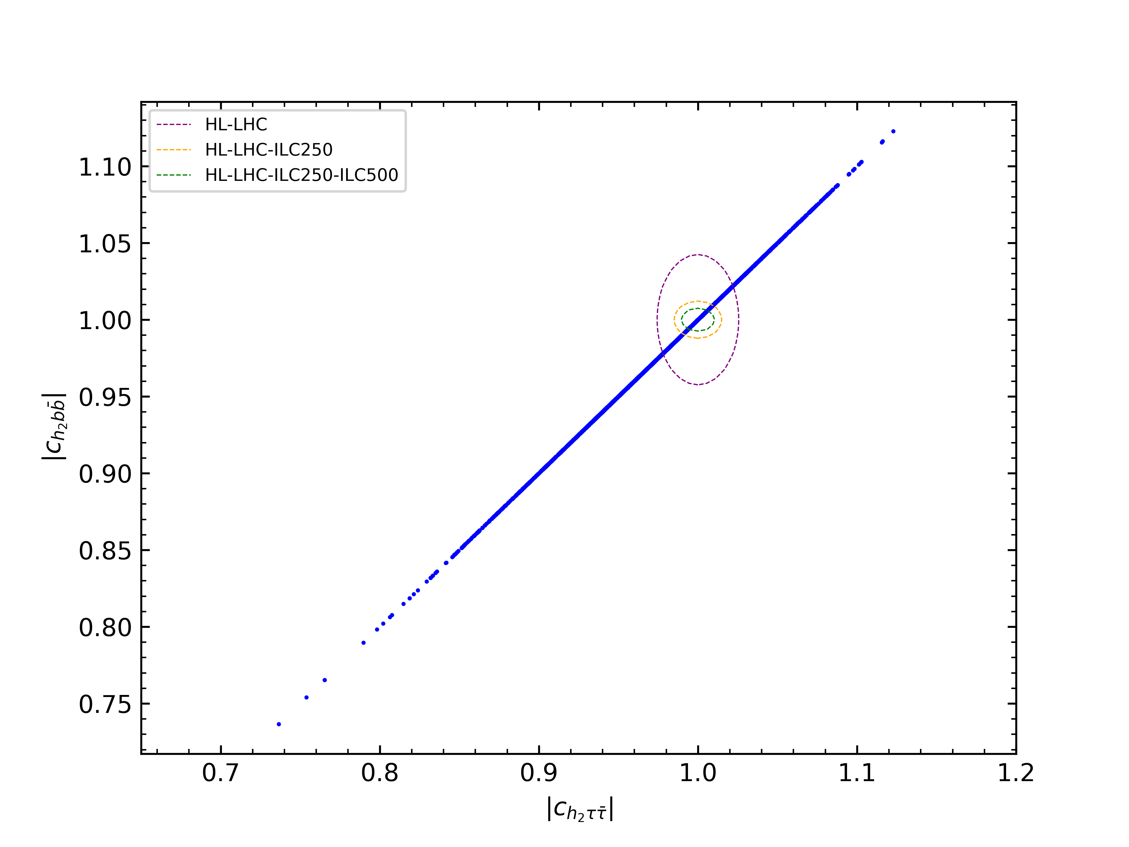
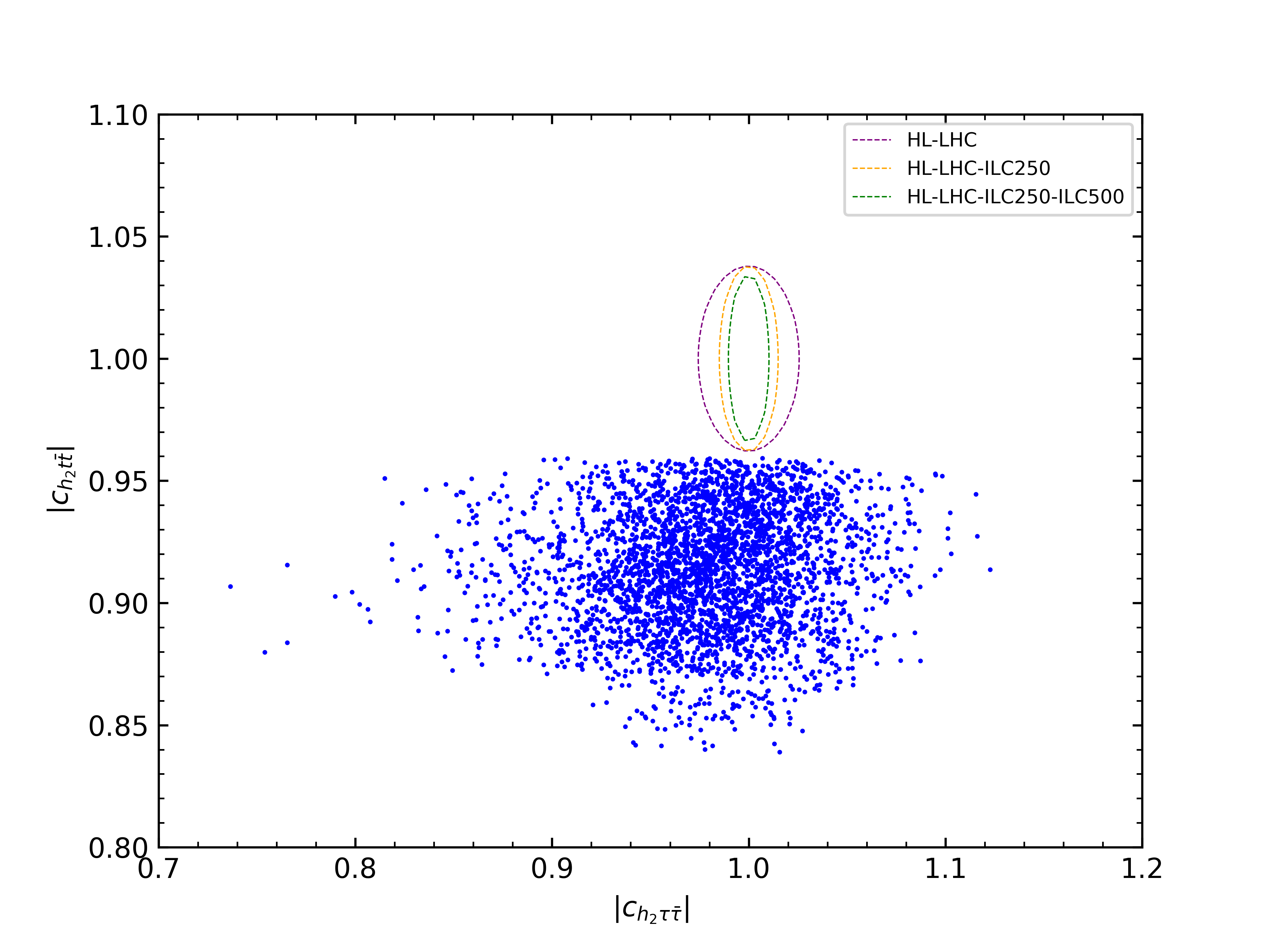
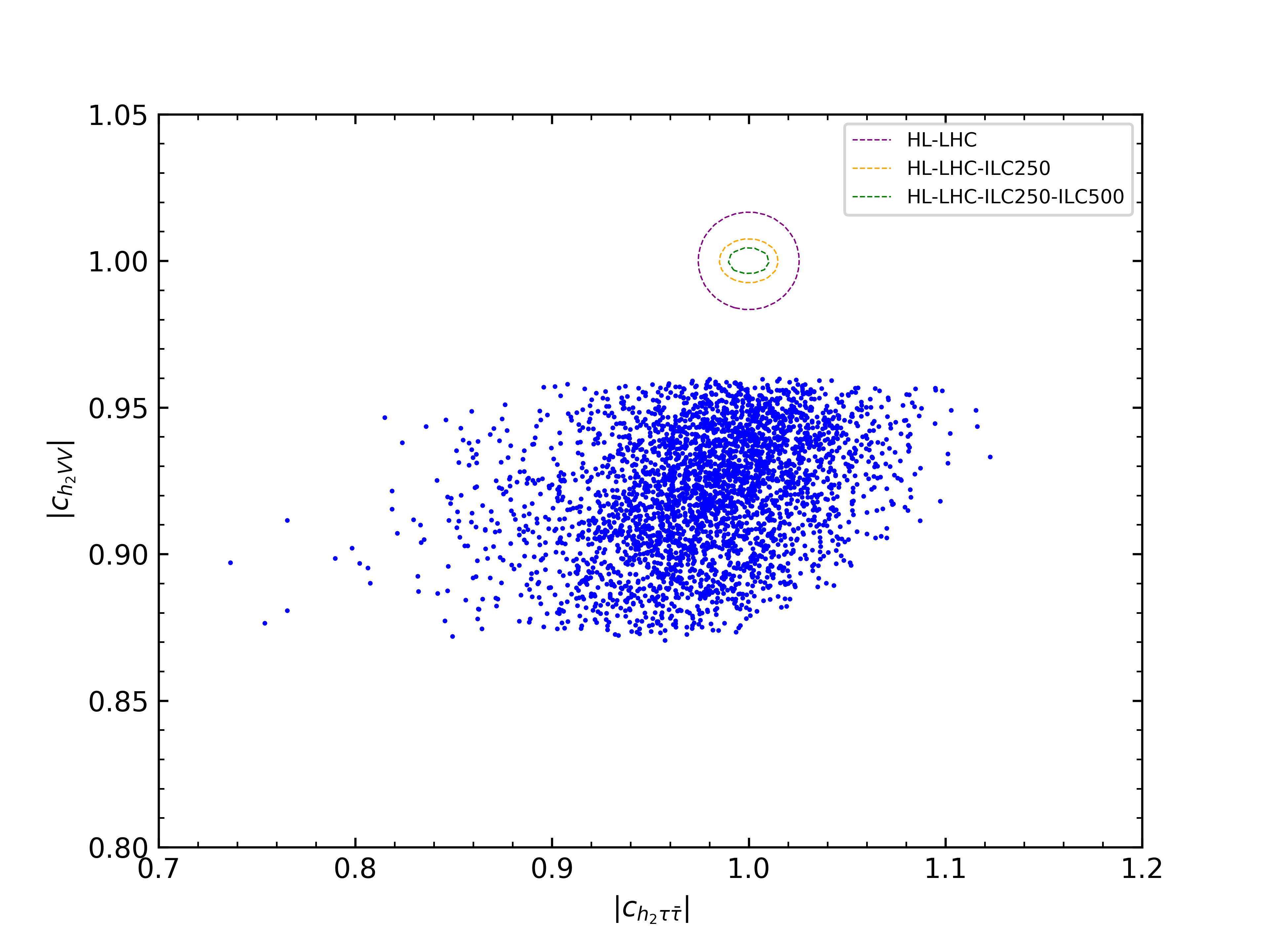
Figure 1: Prospects for the Higgs coupling measurements at the HL-LHC and the ILC (see text). The upper, middle and lower plot show the planes of $|c_{h_{2}\tau\tau}|-|c_{h_{2}t\bar{t}}|$, $|c_{h_{2}\tau\tau}|-|c_{h_{2}b\bar{b}}|$,$|c_{h_{2}\tau\tau}|-|c_{h_{2}VV}|$

In Fig. 1 we plot the coupling modifier of the SM-like Higgs boson $h_{2}$ to $\tau$-leptons, $c_{h_{2}\tau\tau}$ on the horizontal axis against the coupling coefficient to $b$-quarks, $c_{h_{2}b\bar{b}}$ (top), to $t$-quarks, $c_{h_{2}t\bar{t}}$ (middle) and to the massive SM gauge bosons, $c_{h_{2}VV}$ (bottom). These points passed all the experimental and theoretical constraints and have $\chi^{2}_{\text{CMS-LEP}}\leq 2.3$. We include several future precisions for the coupling measurements. It should be noted that they are centered around the SM predictions to show the potential to discriminate the SM from the 2HDMS. The magenta ellipse in each plot shows the expected precision of the measurement of the coupling coefficients at the $1\,\sigma$-level at the HL-LHC from Ref. [50]. The current uncertainties and the HL-LHC analysis are based on the coupling modifier, or $\kappa$-framework. These modifiers are then constrained using a global fit to projected HL-LHC data assuming no deviation from the SM prediction will be found. We use the uncertainties given under the assumptions that no decay of the SM-like Higgs boson to BSM particles is present, and that current systematic uncertainties will be reduced in addition to the reduction of statistical uncertainties due to the increased statistics. The green and the orange ellipses show the corresponding expected uncertainties when the HL-LHC results are combined with projected data from the ILC after the $250\,\,\mathrm{GeV}$ phase and the $500\,\,\mathrm{GeV}$ phase, respectively, taken from Ref. [49]. Their analysis is based on a pure effective field theory calculation, supplemented by further assumptions to facilitate the combination with the HL-LHC projections in the $\kappa$-framework. In particular, in the effective field theory approach the vector boson couplings can be modified beyond a simple rescaling. This possibility was excluded by recasting the fit setting two parameters related to the couplings to the $Z$-boson and the $W$-boson to zero (details can be found in Ref. [49]).

The future precision in the Higgs coupling measurement to quarks can be summarized as follows. The uncertainty of the coupling to $b$-quarks will shrink below $4\%$ at the HL-LHC and below $1\%$ at the ILC. The coupling to $\tau$-leptons an uncertainty at the level of $2\%$ is expected at the HL-LHC. Here, the ILC could reduce this uncertainty to below $1\%$. The coupling to $t$-quarks are expected to reduce the uncertainty by roughly a factor of three at the HL-LHC, employing, however, theoretical assumptions. At the ILC the accuracy of these couplings cam be substantially improved to be model-independent.

In the top plot the 2HDMS points lie on a diagonal line, because in type II models the coupling to leptons and to down-type quarks scale identically. This diagonal goes through the SM prediction ($c_{h_{2}\tau\tau}=c_{h_{2}bb}=1$). While current constraints on the SM-like Higgs-boson properties allow for large deviations of the couplings of up to $40\%$, the parameter space of our scans that is still allowed will be significantly reduced by the expected measurements at the HL-LHC and the ILC. The couplings of the $125\,\,\mathrm{GeV}$ Higgs boson to $t$ quarks, shown in the middle plot of Fig. 1, on the other hand show a deviation from the SM prediction for all points. The deviation ranges from $\sim 1.5\,\sigma$ to about $\sim 4\,\sigma$.

Finally, in the lower plot of Fig. 1, where we show the absolute value of the coupling modifier of the SM-like Higgs boson w.r.t. the vector boson couplings $|c_{h_{2}VV}|$, the parameter points of the 2HDMS show a deviation from the SM prediction substantially larger than the projected experimental uncertainty at HL-LHC and ILC. A $2-3\,\sigma$ deviation from the SM prediction is expected with HL-LHC accuracy. At the ILC a deviation of more than $5\,\sigma$ would be visible. Consequently, the 2HDMS explaining the two excesses in the low-mass Higgs boson searches at LEP and CMS at $\sim 96\,\,\mathrm{GeV}$, can be distinguished from the SM by the measurements of the $125\,\,\mathrm{GeV}$ Higgs-boson couplings at the ILC.

5 Conclusions

The possibility of the 2HDMS explaining both the CMS and the LEP excesses at $\sim 96\,\,\mathrm{GeV}$ simultaneously offers interesting prospects to be probed experimentally. Here we have focused on the possibilities to measure the properties of the $125\,\,\mathrm{GeV}$ Higgs boson at future $e^{+}e^{-}$ colliders. Concretely, we used the projected accuracies of the ILC running at $\sqrt{s}=250\,\,\mathrm{GeV}$ and $500\,\,\mathrm{GeV}$, similar results are expected for CLIC, FCC-ee or CEPC. We analyzed such points that are in agreement with all experimental and theoretical constraints and have $\chi^{2}_{\text{CMS-LEP}}\leq 2.3$ (i.e. they accomodate the two excesses at the $1\,\sigma$ level). These points show a deviation from the prediction of the SM Higgs boson that can clearly be detected by the ILC coupling measurements. While part of the 2HDMS spectrum reproduces the SM coupling to $b$ quarks, the coupling to $t$ quarks deviates between $\sim 1.5$ and $\sim 4\,\sigma$ from the SM prediction. By measuring the coupling to the massive SM gauge bosons, a deviation of more than $5\,\sigma$ is expected. Thus, the 2HDMS explaining the excesses in the Higgs boson searches at LEP and CMS at $\sim 96\,\,\mathrm{GeV}$, can clearly be distinguished from the SM at the ILC.

Acknowledgements

We thank T. Biekötter for very constructive discussions on the N2HDM results. The work of S.H. is supported in part by the MEINCOP Spain under contract PID2019-110058GB-C21 and in part by the AEI through the grant IFT Centro de Excelencia Severo Ochoa SEV-2016-0597. C. L., G.M.-P. and S.P.  acknowledge the support by the Deutsche Forschungsgemeinschaft (DFG, German Research Foundation) under Germany’s Excellence Strategy – EXC 2121 “Quantum Universe – 390833306.”

References

- [1] G. Aad et al. [ATLAS Collab.], Phys. Lett. B 716 (2012) 1 [arXiv:1207.7214 [hep-ex]].
- [2] S. Chatrchyan et al. [CMS Collab.], Phys. Lett. B 716 (2012) 30 [arXiv:1207.7235 [hep-ex]].
- [3] G. Aad et al. [ATLAS and CMS Collaborations], JHEP 1608 (2016) 045 [arXiv:1606.02266 [hep-ex]].
- [4] R. Barate et al. [LEP Working Group for Higgs boson searches, ALEPH, DELPHI, L3 and OPAL], Phys. Lett. B 565 (2003), 61-75 [arXiv:hep-ex/0306033 [hep-ex]].
- [5] A. M. Sirunyan et al. [CMS Collaboration], Phys. Lett. B 793 (2019), 320-347 [arXiv:1811.08459 [hep-ex]].
- [6] [CMS Collaboration], CMS-PAS-HIG-14-037.
- [7] S. Heinemeyer and T. Stefaniak, PoS CHARGED2018 (2019), 016 [arXiv:1812.05864 [hep-ph]].
- [8] T. Biekötter, M. Chakraborti and S. Heinemeyer, PoS CORFU2018 (2019), 015 [arXiv:1905.03280 [hep-ph]].
- [9] T. Biekötter, M. Chakraborti and S. Heinemeyer, [arXiv:1910.06858 [hep-ph]].
- [10] T. Biekötter, M. Chakraborti and S. Heinemeyer, [arXiv:2002.06904 [hep-ph]].
- [11] C. Y. Chen, M. Freid and M. Sher, Phys. Rev. D 89 (2014) no.7, 075009 [arXiv:1312.3949 [hep-ph]].
- [12] M. Mühlleitner, M. O. P. Sampaio, R. Santos and J. Wittbrodt, JHEP 03 (2017), 094 [arXiv:1612.01309 [hep-ph]].
- [13] T. Biekötter, S. Heinemeyer and C. Muñoz, Eur. Phys. J. C 78 (2018) no.6, 504 [arXiv:1712.07475 [hep-ph]].
- [14] F. Domingo, S. Heinemeyer, S. Paßehr and G. Weiglein, Eur. Phys. J. C 78 (2018) no.11, 942 [arXiv:1807.06322 [hep-ph]].
- [15] W. G. Hollik, S. Liebler, G. Moortgat-Pick, S. Paßehr and G. Weiglein, Eur. Phys. J. C 79 (2019) no.1, 75 [arXiv:1809.07371 [hep-ph]].
- [16] K. Choi, S. H. Im, K. S. Jeong and C. B. Park, Eur. Phys. J. C 79 (2019) no.11, 956 [arXiv:1906.03389 [hep-ph]].
- [17] T. Biekötter, S. Heinemeyer and C. Muñoz, Eur. Phys. J. C 79 (2019) no.8, 667 [arXiv:1906.06173 [hep-ph]].
- [18] J. Cao, X. Jia, Y. Yue, H. Zhou and P. Zhu, Phys. Rev. D 101 (2020) no.5, 055008 [arXiv:1908.07206 [hep-ph]].
- [19] S. Heinemeyer, Int. J. Mod. Phys. A 33 (2018) no.31, 1844006.
- [20] F. Richard, [arXiv:2001.04770 [hep-ex]].
- [21] S. Heinemeyer, C. Li, F. Lika, G. Moortgat-Pick and S. Paasch, in preparation.
- [22] T. Biekötter, M. Chakraborti and S. Heinemeyer, [arXiv:2003.05422 [hep-ph]].
- [23] Margarete Mühlleitner, Marco O. P. Sampaio, Rui Santos, and Jonas Wittbrodt, 2020 [arXiv:2007.02985 [hep-ph]].
- [24] J. Horejsi and M. Kladiva, Eur. Phys. J. C 46 (2006), 81-91 [arXiv:hep-ph/0510154 [hep-ph]].
- [25] K.G. Klimenko, Theor. Math. Phys. 62, 58-65, (1985) [Teor. Mat.Fiz.62,87(1985)].
- [26] W. G. Hollik, G. Weiglein and J. Wittbrodt, JHEP 03 (2019), 109 [arXiv:1812.04644 [hep-ph]].
- [27] P. M. Ferreira, M. Mühlleitner, R. Santos, G. Weiglein and J. Wittbrodt, JHEP 09 (2019), 006 [arXiv:1905.10234 [hep-ph]].
- [28] J. Wittbrodt, see: https://gitlab.com/jonaswittbrodt/EVADE
- [29] P. Bechtle, S. Heinemeyer, O. Stål, T. Stefaniak and G. Weiglein, Eur. Phys. J. C 74 (2014) no.2, 2711 [arXiv:1305.1933 [hep-ph]].
- [30] P. Bechtle, S. Heinemeyer, O. Stål, T. Stefaniak and G. Weiglein, JHEP 1411 (2014) 039 [arXiv:1403.1582 [hep-ph]].
- [31] P. Bechtle, S. Heinemeyer, T. Klingl, T. Stefaniak, G. Weiglein and J. Wittbrodt, Eur. Phys. J. C 81 (2021) no.2, 145 [arXiv:2012.09197 [hep-ph]].
- [32] P. Bechtle, O. Brein, S. Heinemeyer, G. Weiglein and K. E. Williams, Comput. Phys. Commun. 181 (2010) 138 [arXiv:0811.4169 [hep-ph]].
- [33] P. Bechtle, O. Brein, S. Heinemeyer, G. Weiglein and K. E. Williams, Comput. Phys. Commun. 182 (2011) 2605 [arXiv:1102.1898 [hep-ph]].
- [34] P. Bechtle, O. Brein, S. Heinemeyer, O. Stål, T. Stefaniak, G. Weiglein and K. E. Williams, Eur. Phys. J. C 74 (2014) no.3, 2693 [arXiv:1311.0055 [hep-ph]].
- [35] P. Bechtle, S. Heinemeyer, O. Stål, T. Stefaniak and G. Weiglein, Eur. Phys. J. C 75 (2015) no.9, 421 [arXiv:1507.06706 [hep-ph]].
- [36] P. Bechtle, D. Dercks, S. Heinemeyer, T. Klingl, T. Stefaniak, G. Weiglein and J. Wittbrodt, Eur. Phys. J. C 80 (2020) no.12, 1211 [arXiv:2006.06007 [hep-ph]].
- [37] A. Arbey, F. Mahmoudi, O. Stål and T. Stefaniak, Eur. Phys. J. C 78 (2018) no.3, 182 [arXiv:1706.07414 [hep-ph]].
- [38] J. Haller, A. Hoecker, R. Kogler, K. Mönig, T. Peiffer and J. Stelzer, Eur. Phys. J. C 78 (2018) no.8, 675 [arXiv:1803.01853 [hep-ph]].
- [39] M. E. Peskin and T. Takeuchi, Phys. Rev. Lett. 65 (1990) 964.
- [40] M. E. Peskin and T. Takeuchi, Phys. Rev. D 46 (1992) 381.
- [41] G. Funk, D. O’Neil and R. M. Winters, Int. J. Mod. Phys. A 27 (2012) 1250021 [arXiv:1110.3812 [hep-ph]].
- [42] T. Biekötter, M. Chakraborti and S. Heinemeyer, Eur. Phys. J. C 80 (2020) no.1, 2 [arXiv:1903.11661 [hep-ph]].
- [43] W. Porod and F. Staub, Comput. Phys. Commun. 183 (2012), 2458-2469 [arXiv:1104.1573 [hep-ph]].
- [44] W. Porod, Comput. Phys. Commun. 153 (2003), 275-315 [arXiv:hep-ph/0301101 [hep-ph]].
- [45] P. Drechsel, G. Moortgat-Pick and G. Weiglein, Eur. Phys. J. C 80 (2020) no.10, 922 [arXiv:1801.09662 [hep-ph]].
- [46] [ATLAS Collaboration], ATLAS-CONF-2018-031.
- [47] A. M. Sirunyan et al. [CMS Collaboration], Eur. Phys. J. C 79 (2019) no.5, 421 [arXiv:1809.10733 [hep-ex]].
- [48] S. Dawson et al. [arXiv:1310.8361 [hep-ex]].
- [49] P. Bambade et al., [arXiv:1903.01629 [hep-ex]].
- [50] M. Cepeda et al., CERN Yellow Rep. Monogr. 7 (2019), 221-584 [arXiv:1902.00134 [hep-ph]].