Interplay Between NOMA and GSSK: Detection Strategies and Performance Analysis

Abstract

Non-orthogonal multiple access (NOMA) is a technology enabler for the fifth generation and beyond networks, which has shown a great flexibility such that it can be readily integrated with other wireless technologies. In this paper, we investigate the interplay between NOMA and generalized space shift keying (GSSK) in a hybrid NOMA-GSSK (N-GSSK) network. Specifically, we provide a comprehensive analytical framework and propose a novel suboptimal energy-based maximum likelihood (ML) detector for the N-GSSK scheme. The proposed ML decoder exploits the energy of the received signals in order to estimate the active antenna indices. Its performance is investigated in terms of pairwise error probability, bit error rate union bound, and achievable rate. Finally, we establish the validity of our analysis through Monte-Carlo simulations and demonstrate that N-GSSK outperforms conventional NOMA and GSSK, particularly in terms of spectral efficiency.

I Introduction

The unprecedented growth of mobile data traffic and the massive number of connected devices, due to the emergence of internet of things (IoT), have posed several challenges for the fifth generation and beyond networks, such as high spectral efficiency, massive connectivity, and requirements for low latency. Accordingly, several promising technologies have been proposed to address these stringent requirements, including massive multiple-input multiple-output (MIMO) [1, 2], millimetre wave (mmWave) communications [3, 4, 5, 6], and spatial modulation (SM) techniques [7], which enable information transmission through spatial and signal constellation [8, 9, 10].

As a key enabling technology for the fifth generation and beyond networks networks, non-orthogonal multiple access (NOMA) is envisioned to increase the system throughput and support massive connectivity [2]. It is worth noting that NOMA can be classified into two different approaches: (a) power domain [11], and (b) code domain [12]. In the power domain NOMA, users are assigned different power levels over the same time and frequency resources. On the contrary, in the code domain NOMA, multiplexing is carried out using spreading sequences with low cross-correlation, similar to code division multiple access technology. The basic principle of NOMA is to allow multiple users to share the same frequency and time resources while controlling the level of inter-user interference [11]. Unlike conventional orthogonal multiple access (OMA) techniques, where users in a cell are assigned dedicated communication resources, e.g., time, frequency or code, NOMA employs superposition coding, where multiple users are multiplexed in the power domain at the transmitter side. At the users’ terminals, multi-user detection is realized by successive interference cancellation (SIC). It has been demonstrated in the recent literature that NOMA outperforms OMA in several aspects such as spectral efficiency, which is realized by serving multiple users at the same time and frequency resource block, interference mitigation through SIC, and support for massive connectivity [13]. Furthermore, users in NOMA do not require a prescheduled time slot structure; hence, NOMA offers lower latency. Moreover, NOMA can ensure user-fairness and diverse quality-of-service by employing flexible power control strategies between strong and weak users [11].

On the other hand, SM, which is considered as a promising MIMO technique for the fifth generation and beyond networks wireless networks, has received significant attention in the recent literature. In SM, information bits are divided into blocks, each of which consists of two subblocks. The first subblock maps the information bits to an arbitrary signal constellation, whereas the second subblock determines the index of the transmit antenna to be used for transmission [14]. In order to reduce the system’s complexity, space shift keying (SSK) modulation, which is a variant of spatial modulation, was introduced in [15]. The key idea of SSK is the activation of one antenna at each symbol duration, which cleverly sends source information to a receiver while removing the effects of inter-antenna interference. Since SSK avoids modulation/demodulation of data symbols, the complexity of the system is significantly reduced but at the cost of a reduced spectral efficiency. To address this concern, generalized space shift keying (GSSK) modulation was proposed in [16], [17]. Unlike SSK, GSSK allows for more than one active antenna at each symbol duration, resulting in a better spectral efficiency but at the cost of additional receiver complexity.

The integration of NOMA with other physical layer techniques such as cooperative communication [18, 19, 20, 21, 22] and MIMO[23], has received a significant attention recently. In [22], a new simultaneous wireless information and power transfer NOMA scheme was proposed. NOMA-enabled cognitive radio networks and NOMA in vehicle-to-vehicle massive MIMO channels were investigated in [24] and [25], respectively. The aforementioned studies have focused on the outage and sum rate analysis, and demonstrated that NOMA outperforms other conventional OMA schemes.

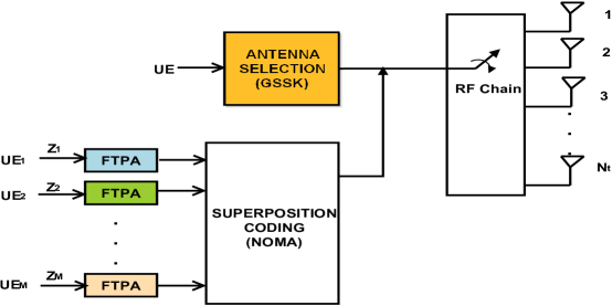
Figure 1: Transmitter model of N-GSSK.

I-A Related Work

Extensive research efforts have been made towards investigating the performance of NOMA from different perspectives, and under various scenarios. Liu et al. [26] studied the performance of a heterogeneous network with coordinated joint transmission-NOMA in order to enhance the performance of the farthest user in a cell. This scheme was shown to significantly enhance the coverage and throughput performances of all users, especially in dense networks. Ali et al. [27] formulated a joint optimization problem for the sum-throughput maximization under several constraints, i.e., transmission power budget, minimum rate requirements, and operational SIC requirements. The work in [28] focused on throughput enhancement. The authors in [29] demonstrated that NOMA requires a longer downlink wireless energy transfer time duration than TDMA, which implies that NOMA is less energy efficient, particularly in those scenarios where energy consumption is of great importance [30]. The authors in [31] investigated a system which incorporates both NOMA and OMA in a unified framework. It was shown that the proposed NOMA-OMA scheme outperforms NOMA- and OMA-only in terms of spectral and energy efficiency trade-off and user fairness. However, it suffers from a level of inter-user interference and relatively high computational complexity.

Figure 2: Receiver model of N-GSSK.

The integration of NOMA with SM has been recently investigated in the literature [7]. In [32], a hybrid detection technique was introduced, which combines NOMA and SM in an uplink transmission scenario. It was shown that the combination of SM and NOMA offers promising spectral efficiency enhancements. Likewise, spectral efficiency analysis was considered in [33, 34] in order to characterize the performance of spatially-modulated NOMA under different transmission scenarios. More recently, the work of [35] proposed a NOMA-SM system in order to quantify the trade-off between spectral efficiency and interference mitigation. User pairing for NOMA-SM was also addressed in [35], where the performance of NOMA-SM was compared with OMA-SM as well as transmit antenna grouping-based SM (TAG-SM). The performance gains of NOMA-SM was further quantified. However, in the aformentioned works, the number of users in a resource block was restricted to two.

The combination of NOMA with SSK was considered in [36] for a three-user scenario, where a cell edge user was served using SSK modulation and the other two users served using NOMA. This work was generalized in [37] by integrating NOMA with GSSK to accommodate more users. It was shown that NOMA-GSSK achieves higher spectral efficiency and lower bit error rate (BER) when compared with conventional GSSK (c-GSSK), conventional NOMA (c-NOMA), and NOMA-SSK systems. This is primarily due to the fact that users are multiplexed in power and spatial domain.

I-B Motivation

To the best of authors’ knowledge, the only existing work that combines NOMA with GSSK systems was reported in [37], which is called here ideal-NOMA-GSSK (iN-GSSK). Although this work is interesting and paves the way for further advancements in this area, it has the following limitations. First, the maximum likelihood (ML) detector at the cell-edge users (GSSK users) is designed under the assumption of perfect knowledge of NOMA signals. Consequently, the introduced detector and the corresponding analysis turned out to be similar to that of c-GSSK. Second, the proposed framework assumes perfect SIC. It also assumes perfect knowledge of active antenna indices at NOMA users. These are clearly unrealistic assumptions, particularly in practical scenarios. Third, the detrimental effect of fading on the performance of both GSSK and NOMA users was not discussed.

In summary, the work in [37] treats NOMA and GSSK users independently and does not provide a holistic view of the practical considerations on the integration of NOMA and GSSK schemes.

I-C Contributions

Motivated by the limitations of iN-GSSK [37] and the lack of a general theoretic framework for NOMA-GSSK (henceforth called N-GSSK), we introduce, in this work, a framework for the design and analysis of N-GSSK over fading channels. In particular, we introduce an analytical framework that investigates the performance of N-GSSK by explicitly multiplexing information in the spatial and power domains. We relax the assumption of perfect knowledge of NOMA signals at GSSK users, and present a novel, energy-based ML detector for GSSK signals. Additionally, we derive expressions for the pairwise error probability (PEP) and bit error rate (BER) union bound of the proposed detector. To summarize, the main contributions of this paper are as follows.

• We propose a novel energy-based ML detection strategy for the detection of GSSK signals, which does not require the knowledge of NOMA signals. We further demonstrate that the performance of N-GSSK users with energy-based ML detection asymptotically converges to that of iN-GSSK.

• We derive a tight approximation for the pairwise error probability (PEP) of GSSK users over Rayleigh fading channels and establish the tightness of the approximation through Monte Carlo simulations and numerical results.

• We derive a novel expression for the overall BER of NOMA users, taking in account the BER of the active antenna index detection.

• We evaluate the spectral efficiency of the proposed N-GSSK with imperfect SIC, and demonstrate that it outperforms the c-GSSK scheme.

I-D Organization

The remainder of this paper is organized as follows. Section II presents the N-GSSK system model . The detection techniques of GSSK and NOMA users are investigated in Section III. The performance analysis in terms of PEP, BER and spectral efficiency for GSSK and NOMA users is presented in Section IV. Section V validates the theoretical analysis through numerical and Monte Carlo simulations results. C oncluding remarks are provided in Section VI.

II System Model

We consider a network with a base station (BS) equipped with $N_{t}$ transmit antennas, serving a group of single antenna-equipped users, denoted by $\text{UE}_{\scriptscriptstyle 0},\text{UE}_{\scriptscriptstyle 1},\text{UE}_{\scriptscriptstyle 2},\ldots,\text{UE}_{\scriptscriptstyle M}$. As illustrated in Fig. 1, the BS generates sequences of independent bits, which are then mapped to constellation points in a GSSK constellation diagram. In GSSK modulation, $n_{t}$ out of $N_{t}$ antennas made active at a given transmission slot. Without loss of generality, we assume that $\text{UE}_{\scriptscriptstyle 0}$ represents the GSSK user, whereas other users are assigned to the NOMA network. Note that the non-zero elements in the GSSK symbols represent the superposition coded symbols of NOMA users.

At the receiving end, $\text{UE}_{\scriptscriptstyle 0}$ employs maximum-likelihood (ML) detection to find the indices of active antennas, and decode the corresponding transmitted symbols, see Fig. 2. Since the information is encoded onto the spatial-constellation diagram, the decoder of $\text{UE}_{\scriptscriptstyle 0}$ searches over all possible active antenna combinations to obtain an estimates of the antenna indices [38]. The rest of the users, i.e., $\text{UE}_{\scriptscriptstyle 1},\text{UE}_{\scriptscriptstyle 2},\ldots,\text{UE}_{\scriptscriptstyle M}$, which are multiplexed in the power domain based on the principle of SC and fractional transmit power allocation (FTPA), employ GSSK detection followed by SIC.

In summary, in the N-GSSK scheme, the information corresponding to the GSSK user is spatially modulated over $n_{t}$ antennas, each of which carry a NOMA signal, which is intended to NOMA users. Hence, by accommodating NOMA users in a GSSK system, the overall spectral efficiency of the considered network is improved.

Let the effective channel gain over $n_{t}$ active transmit antennas at user $\text{UE}_{\scriptscriptstyle 0}$ be denoted by $\left|h_{j,\text{eff}}\right|$. Without loss of generality, let the effective channel gains of NOMA users be sorted in an increasing order, and given as $\left|g_{1,\text{eff}}\right|<\left|g_{2,\text{eff}}\right|<\ldots<\left|g_{M,\text{eff}}\right|$[39]. The signal transmitted from the BS for $M$ NOMA users is given by

$$X=\sum_{m=1}^{M}\sqrt{\alpha_{m}P}\leavevmode\nobreak\ z_{m},$$ (1)

where $P$ is the transmit power, $\alpha_{m}>0$ is the power allocation coefficient, $z_{m}$ is the transmitted symbol corresponding to the $m^{\text{th}}$ NOMA user, and $\sum_{m=1}^{M}\alpha_{m}=1$. Note that the power allocation coefficients are sorted in a descending order. i.e., $\alpha_{1}>\alpha_{2}>\cdots>\alpha_{M}$. We assume the symbol $z_{m}$ is drawn from a constant-modulus constellation, such as phase shift keying (PSK) [40]. As mentioned earlier, the superimposed symbol $X$ is transmitted through a specific combination out of $M_{H}={N_{t}\choose n_{t}}$ different combinations (i.e., possible constellation points), which are selected based on a predefined GSSK antenna mapping rule.

In c-GSSK, a random sequence of independent bits is fed into a GSSK mapper, where groups of bits are mapped to symbols in the spatial constellation diagram, which in turns activates a set of transmit antennas [41]. Typically, each active antenna transmits a constant signal $1/\sqrt{n_{t}}$. However, in the considered N-GSSK system, the symbol $X/\sqrt{(n_{t})}$ is transmitted over $n_{t}$ antennas with a total transmit power of $P$, similar to the generalized spatial modulation (GSM)[42]. In other words, the transmitted signal on the $N_{t}\times 1$ antenna array is given by

$$\left[\frac{X}{\sqrt{n_{t}}}\leavevmode\nobreak\ 0\leavevmode\nobreak\ \cdots\leavevmode\nobreak\ 0\leavevmode\nobreak\ \frac{X}{\sqrt{n_{t}}}\leavevmode\nobreak\ \cdots\leavevmode\nobreak\ 0\right],$$ (2)

where the non-zero elements represent the active antennas $n_{t}$. Clearly, the signal received at the GSSK user is given by [9]

$$y_{0}=\sqrt{\rho^{\prime}}h_{j,\text{eff}}X+w_{0},$$ (3)

where $w_{0}$ is assumed to be a circularly symmetric complex Gaussian (CSCG) random variable with zero mean and variance $\sigma_{n}^{2}$ – denoted by $\mathcal{CN}(0,\sigma_{n}^{2})$ and $h_{j,\text{eff}}=h_{j,1}+h_{j,2}+...+h_{j,n_{t}}$, where $j\in\{1,2,...,M_{H}\}$ denotes the antenna combination for a given GSSK symbol. The fading coefficients $h_{j,i}$ represent the channel gains from the $i^{\rm th}$ active antenna to the GSSK user, where each of which is modeled as complex Gaussian random variable with zeros mean and unit variance, i.e., $\mathcal{CN}(0,1)$.

Without loss of generality, we assume that $\sigma_{n}^{2}=1$. Also, $\rho^{\prime}\triangleq\rho/n_{t}$, where $\rho$ is the average signal-to-noise ratio (SNR). As explained earlier, the GSSK user decodes its transmitted symbols by estimating the antenna indices using an ML decoder. NOMA users, on the other hand, performs GSSK decoding as wel as SIC to decode their own messages. In the considered system model, it is to be noted that although NOMA users receive superimposed signals from multiple antennas, they do not exploit any of the known MIMO-NOMA techniques [43].

III Detection Strategies

In this section, we propose an energy-based ML detector for GSSK detection, which also used for antenna indices estimation required by NOMA users.

III-A Energy-Based ML Detector for the GSSK User

In iN-GSSK, GSSK users are assumed to have perfect knowledge of the NOMA signal $X$. Subsequently, conventional ML decoding is used to estimate the set of active antennas [37]. However, this assumption is unrealistic and impractical. Motivated by this, our proposed decoder first estimates the energy of the received signal as follows:

$$y_{\scriptscriptstyle E}^{\scriptscriptstyle(0)}\triangleq\left|y_{0}\right|^{2}=(\sqrt{\rho^{\prime}}h_{j,\text{eff}}X+w_{0})(\sqrt{\rho^{\prime}}h_{j,\text{eff}}X+w_{0})^{*}$$

$$\leavevmode\nobreak\ \leavevmode\nobreak\ \leavevmode\nobreak\ \leavevmode\nobreak\ \leavevmode\nobreak\ \leavevmode\nobreak\ \leavevmode\nobreak\ \leavevmode\nobreak\ \leavevmode\nobreak\ \leavevmode\nobreak\ \leavevmode\nobreak\ \leavevmode\nobreak\ \leavevmode\nobreak\ =\rho^{\prime}P\left|h_{j,\text{eff}}\right|^{2}+$$

$$\leavevmode\nobreak\ \leavevmode\nobreak\ \leavevmode\nobreak\ \leavevmode\nobreak\ \leavevmode\nobreak\ \leavevmode\nobreak\ \leavevmode\nobreak\ \leavevmode\nobreak\ \leavevmode\nobreak\ \leavevmode\nobreak\ \leavevmode\nobreak\ \leavevmode\nobreak\ \leavevmode\nobreak\ \leavevmode\nobreak\ \leavevmode\nobreak\ \leavevmode\nobreak\ \underbrace{\sqrt{\rho^{\prime}}Xh_{j,\text{eff}}w_{0}^{*}+\sqrt{\rho^{\prime}}X^{*}h_{j,\text{eff}}^{*}w_{0}+|w_{0}|^{2}}_{\text{Interference + Noise}\leavevmode\nobreak\ \triangleq\leavevmode\nobreak\ W_{0}}$$ (4)

$$\leavevmode\nobreak\ \leavevmode\nobreak\ \leavevmode\nobreak\ \leavevmode\nobreak\ \leavevmode\nobreak\ \leavevmode\nobreak\ \leavevmode\nobreak\ \leavevmode\nobreak\ \leavevmode\nobreak\ \leavevmode\nobreak\ \leavevmode\nobreak\ \leavevmode\nobreak\ =\rho^{\prime}P\left|h_{j,\text{eff}}\right|^{2}+W_{0}.$$ (5)

The exact distribution of $W_{0}$ is intractable and difficult to obtain. However, $W_{0}$ in (5) can be approximated as a complex Gaussian random variable with mean $\mu_{I}$ and variance $\sigma_{I}^{2}$, that is, $\mathcal{N}(\mu_{I},\sigma_{I}^{2})$. It can be readily shown that $\mu_{I}=\sigma_{n}^{2}$, and $\sigma_{I}^{2}=\sigma_{n}^{2}[2\rho^{\prime}Pn_{t}+\sigma_{n}^{2}]$. Therefore, the proposed energy-based ML detector at the GSSK user estimates the active antenna indices as follows:

$$\hat{\mathbf{k}}=\underset{k\in\{1,2,...,M_{H}\}}{\arg\min}\left\|y_{\scriptscriptstyle E}^{\scriptscriptstyle(0)}-\rho^{\prime}P\left|h_{k,\text{eff}}\right|^{2}-\mu_{I}\right\|^{2},$$ (6)

where $\hat{\mathbf{k}}$ represents the estimated antenna index vector. It can be readily noticed that the GSSK user does not require the knowledge of the superimposed NOMA signal.

III-B Detection of NOMA Users

As it can be inferred from Fig. 2, GSSK symbols carry both NOMA signals and active antenna indices. Therefore, it is crucial to correctly estimate the set of active antenna indices first in order to reliably decode NOMA signals. Towards this end, NOMA users first perform energy-based GSSK detection, followed by conventional NOMA detection.

The key idea behind NOMA decoding is to employ SIC. In particular, the user with the highest allocated power decodes his own signal by treating interference from other users’ signals as noise. Other users progressively cancel out the decoded signals of lower order users, i.e., users with higher power coefficients, and then decode their own signals while treating signals with lower power values as noise.

The received signal at the $m^{th}$ NOMA user is given by [39]

$$r_{m}=g^{m}_{j,\text{eff}}X+n_{m},\leavevmode\nobreak\ \leavevmode\nobreak\ m=1,2,\ldots,M$$ (7)

where, given the $j^{\rm th}$ set of antenna combination, $g^{m}_{j,\text{eff}}=g^{m}_{j,1}+...+g^{m}_{j,n_{t}}$ denotes the effective channel gain between the BS and the $m^{th}$ user, which is modeled as zero mean complex Gaussian with unit variance and $n_{m}\sim\mathcal{CN}(0,1)$. As noted earlier, the $m^{th}$ user performs SIC by decoding the signals of users with higher power, i.e., $\text{UE}_{\scriptscriptstyle 1},\text{UE}_{\scriptscriptstyle 2},\ldots,\text{UE}_{\scriptscriptstyle m-1}$, while treating the signals of $\text{UE}_{\scriptscriptstyle m+1},\text{UE}_{\scriptscriptstyle m+2},\cdots,\text{UE}_{\scriptscriptstyle M}$, as interference.

IV Performance Analysis

In this section, we present a thorough performance analysis of the detection strategies used by the GSSK and NOMA users, focusing on the error rate analysis and spectral efficiency.

IV-A Bound on BER of the GSSK User

An upper bound on the average BER performance of the GSSK users can be obtained through union bound as [40]

$$P_{\scriptscriptstyle e,GSSK}\leq\frac{1}{M_{H}}\sum_{j=1}^{M_{H}}\sum_{k=1,k\neq j}^{M_{H}}M{(j,k)P(x_{j}\rightarrow x_{k})}$$ (8)

where $M_{H}$ is the set of all possible index sets of active antennas. Note that $b_{H}=\lfloor\log_{2}M_{H}\rfloor$ is the number of bits that can be conveyed by choosing a set of active antennas. Also, $M{(j,k)}$ denotes the number of bits in error between the signals $x_{j}$ and $x_{k}$, and $P(x_{j}\rightarrow x_{k})$ denotes the pairwise error probability (PEP), which represents the probability of erroneously decoding $x_{k}$ when $x_{j}$ was transmitted.

Following the detection strategy proposed in (6), the PEP of the GSSK user conditioned on channel vector can be written as

$$P(x_{j}\rightarrow x_{k}|h_{j,\text{eff}},h_{k,\text{eff}})$$

$$\leavevmode\nobreak\ \leavevmode\nobreak\ =Pr\left(\left|y_{\scriptscriptstyle E}^{\scriptscriptstyle(0)}-\rho^{\prime}P\zeta-\mu_{I}\right|^{2}\leq\left|y_{\scriptscriptstyle E}^{\scriptscriptstyle(0)}-\rho^{\prime}P\xi-\mu_{I}\right|^{2}\right)$$ (9)

$$\leavevmode\nobreak\ \leavevmode\nobreak\ =Pr\left(y_{\scriptscriptstyle E}^{\scriptscriptstyle(0)}>\frac{\rho^{\prime}P}{2}\left[\xi+\zeta\right]+\mu_{I}\right)$$ (10)

where $\xi=\left|h_{j,\text{eff}}\right|^{2}$ and $\zeta=\left|h_{k,\text{eff}}\right|^{2}$. Recalling that $y_{\scriptscriptstyle E}^{\scriptscriptstyle(0)}=\rho^{\prime}P\left|h_{j,\text{eff}}\right|^{2}+W_{j}$, and $W_{j}\sim\mathcal{N}(\sigma_{n}^{2},\sigma_{n}^{2}[2\rho^{\prime}Pn_{t}+\sigma_{n}^{2}])$, (10) can be written as

$$P(x_{j}\rightarrow x_{k}|h_{j,\text{eff}},h_{k,\text{eff}})=Q\left(\frac{\frac{\rho^{\prime}P}{2}d(j,k)}{\sqrt{\sigma_{n}^{2}[2\rho^{\prime}Pn_{t}+\sigma_{n}^{2}]}}\right)$$ (11)

where $d(j,k)\triangleq\left\lvert\xi-\zeta\right\rvert$, and $Q(.)$ is the complementary CDF of a standard Gaussian random variable [40]. The unconditional PEP in (11) can be realized by averaging the conditional PEP over the PDF of $\xi$ and $\zeta$. Noting that $\xi$ and $\xi$ follow the exponential distribution with parameter $\lambda=1/n_{t}$, denoted by $\texttt{Exp}(\lambda)$, the exact PEP of GSSK users can be written as

$$P(x_{j}\rightarrow x_{k})=\int_{0}^{\infty}\int_{0}^{\infty}P(x_{j}\rightarrow x_{k}|h_{j,\text{eff}},h_{k,\text{eff}})\leavevmode\nobreak\$$

$$\leavevmode\nobreak\ \leavevmode\nobreak\ \leavevmode\nobreak\ \leavevmode\nobreak\ \leavevmode\nobreak\ \leavevmode\nobreak\ \leavevmode\nobreak\ \leavevmode\nobreak\ \leavevmode\nobreak\ \leavevmode\nobreak\ \leavevmode\nobreak\ \leavevmode\nobreak\ \leavevmode\nobreak\ \leavevmode\nobreak\ \times f(\xi)f(\zeta)\leavevmode\nobreak\ d\zeta\leavevmode\nobreak\ d\xi,$$ (12)

where $f(\cdot)$ denotes the exponential PDF with parameter $\lambda$. The PEP expression can be further rewritten as

$$P(x_{j}\rightarrow x_{k})=\int_{0}^{\infty}\int_{0}^{\infty}Q\left(\frac{\left|\frac{\rho^{\prime}P\xi}{2}-\frac{\rho^{\prime}P\zeta}{2}\right|}{\sqrt{\sigma_{n}^{2}(2\rho^{\prime}Pn_{t}+\sigma_{n}^{2})}}\right)$$

$$\leavevmode\nobreak\ \leavevmode\nobreak\ \leavevmode\nobreak\ \leavevmode\nobreak\ \leavevmode\nobreak\ \leavevmode\nobreak\ \leavevmode\nobreak\ \leavevmode\nobreak\ \leavevmode\nobreak\ \leavevmode\nobreak\ \leavevmode\nobreak\ \leavevmode\nobreak\ \leavevmode\nobreak\ \leavevmode\nobreak\ \leavevmode\nobreak\ \leavevmode\nobreak\ \leavevmode\nobreak\ \leavevmode\nobreak\ \leavevmode\nobreak\ \leavevmode\nobreak\ \leavevmode\nobreak\ \leavevmode\nobreak\ \leavevmode\nobreak\ \leavevmode\nobreak\ \leavevmode\nobreak\ \leavevmode\nobreak\ \leavevmode\nobreak\ \leavevmode\nobreak\ \leavevmode\nobreak\ \leavevmode\nobreak\ \times\left(\frac{1}{n_{t}}\right)^{2}\exp^{-\frac{(\zeta+\xi)}{n_{t}}}d\xi d\zeta.$$ (13)

The solution to (13) is presented in the following proposition.

Proposition 1.

The PEP of GSSK users is given by (19) on the top of the next page, where $a\triangleq\dfrac{\rho^{\prime}Pn_{t}}{2\sigma_{n}\sqrt{2\rho^{\prime}Pn_{t}+\sigma_{n}^{2}}}$, and $G_{m,n}^{p,q}\left(\cdot\left\lvert\begin{array}[]{c}-\\ -\end{array}\right.\right)$ represents the Meijer G-function.

$$P(x_{j}\rightarrow x_{k})=\dfrac{1}{2}\left[1-\frac{a}{\pi}\left\{\begin{array}[]{c}G_{2,2}^{1,2}\left(2a^{2}\left\lvert\begin{array}[]{c}\frac{1}{2},0;-\\ 0;-\frac{1}{2}\end{array}\right.\right)+\dfrac{1}{4}\sum_{k=0}^{\infty}\dfrac{1}{k!}G_{3,2}^{1,3}\left(\frac{a^{2}}{2}\left\lvert\begin{array}[]{c}\frac{1}{2},-\frac{k}{2},-\frac{1}{2}-\frac{k}{2};-\\ 0;-\frac{1}{2}\end{array}\right.\right)\end{array}\right\}\right]$$ (19)

Proof.

See Appendix. ∎

It is worth noting that the infinite series in (19) converges very fast, and about $20$ terms suffice to obtain an accuracy up to four decimal places. More details are discussed in Sec. V. The PEP expression in (19) constitutes the basic building block for the derivation of the union bound given by (8).

IV-B Bound on BER of NOMA Users

As stated earlier, NOMA users first perform energy-based GSSK detection, followed by conventional NOMA detection. Without loss of generality, we consider the first user as the farthest user. Therefore, the received signal at the first user, conditioned on the $j^{\text{th}}$ set of antenna combinations can be represented as

$$y_{1}=g^{1}_{j,\text{eff}}\left(\sqrt{\alpha_{1}P}z_{1}+\sum_{m=2}^{M}\sqrt{\alpha_{m}P}z_{m}\right)+w_{1}$$ (20)

where $\sum_{m=2}^{M}\sqrt{\alpha_{m}P}z_{m}$ represents the sum of interference terms corresponding to the signals for the other users. Therefore, the conditional PEP for the first user can be represented as [39],

$$P(z_{1}\rightarrow\hat{z}_{1}|g_{1})=$$

$$Q\left(\frac{\sqrt{\alpha_{1}P}g_{1}\left|\delta_{1}\right|^{2}+2g_{1}\text{Re}\left\{\delta_{1}\sum_{j=2}^{M}\sqrt{\alpha_{j}P}z_{j}^{*}\right\}}{\sqrt{2}|\delta_{1}|\sigma_{n}}\right),$$ (21)

where $\delta_{1}=(z_{1}-\hat{z}_{1})$ and $g_{1}=\left\lvert g^{1}_{j,\text{eff}}\right\rvert$. Note that the statistics of $g_{1}$ can be obtained from the order statistics of the Rayleigh distribution. The average PEP over the PDF of $g_{1}$ is given by [39]

$$P(z_{1}\rightarrow\hat{z}_{1})=\frac{1}{2}\left(1-\frac{\nu\sigma_{h}}{\sqrt{2\beta^{2}+\nu^{2}\sigma_{h}^{2}}}\right)$$ (22)

where

$$\nu=\sqrt{\alpha_{1}P}g_{1}\left|\delta_{1}\right|^{2}+2g_{1}\text{Re}\left\{\delta_{1}\sum_{j=2}^{M}\sqrt{\alpha_{j}P}z_{j}^{*}\right\},$$ (23)

$\beta=\sqrt{2}\left|\delta_{1}\right|\sigma_{n}$, and $\sigma_{h}^{2}=\mathbb{E}g_{1}^{2}$. Similarly, the conditional PEP of the $m^{\text{th}}$ user can be evaluated as in [44, Eq. (21)] as

$$P(z_{m}\rightarrow\hat{z}_{m}|g_{m})=Q\left(\frac{g_{m}\eta_{m}}{\sqrt{2}|\delta_{m}|\sigma_{n}}\right),$$ (24)

where $g_{m}=\left\lvert g^{m}_{j,\text{eff}}\right\rvert$ and

$$\eta_{m}=\sqrt{\alpha_{m}P}\left|\delta_{m}\right|^{2}+2\text{Re}\left\{\delta_{m}\sum_{j=m+1}^{M}\sqrt{\alpha_{j}P}\hat{z}_{m}^{*}\right\}$$

$$\leavevmode\nobreak\ \leavevmode\nobreak\ \leavevmode\nobreak\ \leavevmode\nobreak\ \leavevmode\nobreak\ \leavevmode\nobreak\ \leavevmode\nobreak\ \leavevmode\nobreak\ \leavevmode\nobreak\ \leavevmode\nobreak\ \leavevmode\nobreak\ \leavevmode\nobreak\ \leavevmode\nobreak\ \leavevmode\nobreak\ \leavevmode\nobreak\ \leavevmode\nobreak\ \leavevmode\nobreak\ \leavevmode\nobreak\ \leavevmode\nobreak\ \leavevmode\nobreak\ \leavevmode\nobreak\ \leavevmode\nobreak\ \leavevmode\nobreak\ \leavevmode\nobreak\ \leavevmode\nobreak\ +\text{Re}\left\{\delta_{m}\sum_{k=1}^{m-1}\sqrt{\alpha_{k}P}\delta_{k}^{*}\right\},$$

where $\delta_{m}=(z_{m}-\hat{z}_{m})$ and $\delta_{k}=(z_{k}-\hat{z}_{k})$. Following an approach similar to above, the average PEP over the PDF of $g_{m}$ can be written as

$$P(z_{m}\rightarrow\hat{z}_{m})=\frac{M!}{\sigma_{h}^{2}(m-1)!(M-m)!}$$ (25)

$$\leavevmode\nobreak\ \leavevmode\nobreak\ \leavevmode\nobreak\ \leavevmode\nobreak\ \leavevmode\nobreak\ \leavevmode\nobreak\ \leavevmode\nobreak\ \leavevmode\nobreak\ \leavevmode\nobreak\ \leavevmode\nobreak\ \sum_{j=0}^{m-1}\binom{m-1}{j}\frac{(-1)^{2(m-1)-j}}{[M-m+j+1]}$$

$$\leavevmode\nobreak\ \leavevmode\nobreak\ \leavevmode\nobreak\ \leavevmode\nobreak\ \leavevmode\nobreak\ \leavevmode\nobreak\ \leavevmode\nobreak\ \leavevmode\nobreak\ \leavevmode\nobreak\ \leavevmode\nobreak\ \left(1-\frac{\eta_{m}\sigma_{h}}{\sqrt{\eta_{m}^{2}\sigma_{h}^{2}+[M-m+j+1](\sqrt{2}|\delta_{m}|\sigma_{n})^{2}}}\right).$$

Next, the above PEP expression is used to calculate an upper bound on the BER as

$$P_{\scriptscriptstyle e,C-NOMA}^{\scriptscriptstyle(m)}\leq\frac{1}{B}\sum_{\ell=1}^{L}P(z_{\ell}^{(m)})$$

$$\leavevmode\nobreak\ \leavevmode\nobreak\ \leavevmode\nobreak\ \leavevmode\nobreak\ \leavevmode\nobreak\ \leavevmode\nobreak\ \leavevmode\nobreak\ \times\sum_{\ell=1,\leavevmode\nobreak\ z_{\ell}^{(m)}\neq\hat{z}_{\ell}^{(m)}}^{L}q(z_{\ell}^{(m)}\rightarrow\hat{z}_{\ell}^{(m)})P(z_{\ell}^{(m)}\rightarrow\hat{z}_{\ell}^{(m)}),$$ (26)

where $z_{\ell}^{(m)}$ and $\hat{z}_{\ell}^{(m)}$ are the symbols for the $m^{\text{th}}$ user, $L$ is the number of symbols, $B$ is the number of information bits in symbol $z_{\ell}^{(m)}$, $P(z_{\ell}^{(m)})$ is the probability of occurrence of $z_{\ell}^{(m)}$, and $q(z_{\ell}^{(m)}\rightarrow\hat{z}_{\ell}^{(m)})$ is the number of bit errors when $z_{\ell}^{(m)}$ is transmitted and $\hat{z}_{\ell}^{(m)}$ is detected. The overall BER across $M$ NOMA users depends on the BER of the active antenna indices and NOMA detectors, and is given by

$$P_{\scriptscriptstyle e,overall}^{\scriptscriptstyle(NOMA)}\leq(1-P_{\scriptscriptstyle e,GSSK})\sum_{m=1}^{M}P_{\scriptscriptstyle e,C-NOMA}^{\scriptscriptstyle(m)}+P_{\scriptscriptstyle e,GSSK},$$ (27)

and the overall BER for the entire N-GSSK system is given by

$$P_{\scriptscriptstyle e,overall}\leq(1-P_{\scriptscriptstyle e,GSSK})\sum_{m=1}^{M}P_{\scriptscriptstyle e,C-NOMA}^{\scriptscriptstyle(m)}+2P_{\scriptscriptstyle e,GSSK}.$$ (28)

IV-C Sum Rate of N-GSSK

The sum rate of the GSSK user is given by

$$R_{\scriptscriptstyle GSSK}=(1-P_{\scriptscriptstyle e,GSSK})\left\lfloor\log_{2}{N_{t}\choose n_{t}}\right\rfloor.$$ (29)

For NOMA users, the $m^{\text{th}}$ user will detect the $n^{\text{th}}$ users’ message such that $n<m$, by performing SIC. The message from the users $n>m$ will be treated as noise at the $m^{\text{th}}$ user. Accordingly, the average data rate at the $m^{\text{th}}$ user, $m=1,\ldots,M-1$, is given by

$$R_{m}=\int_{0}^{\infty}\log\left(1+\frac{g_{m}^{2}\alpha_{m}P}{g_{m}^{2}\sum_{i=m+1}^{M}\alpha_{i}P+\sigma_{n}^{2}}\right){f}(g_{m})\leavevmode\nobreak\ dg_{m},$$ (30)

where ${f}(g_{m})$ denotes the PDF of $g_{m}$. Similarly, the average rate at the $M^{th}$ user is given by

$$R_{M}=\int_{0}^{\infty}\log\left(1+\frac{g_{M}^{2}\alpha_{M}P}{\sigma_{n}^{2}}\right){f}(g_{M})\leavevmode\nobreak\ dg_{M},$$ (31)

where $g_{M}=\left\lvert g^{M}_{j,\text{eff}}\right\rvert$, and ${f}(g_{M})$ denotes the PDF of $g_{M}$. Therefore, the average sum rate achieved by all $M$ NOMA users is given by

$$R_{\scriptscriptstyle NOMA}=\sum_{m=1}^{M}(1-P_{\scriptscriptstyle e,C-NOMA}^{\scriptscriptstyle(m)})R_{m},$$ (32)

and the total sum rate of N-GSSK system is given by

$$R_{\scriptscriptstyle N-GSSK}=R_{\scriptscriptstyle GSSK}+R_{\scriptscriptstyle NOMA},$$ (33)

which is an improvement over the rate achieved by the c-GSSK system, given in (29). It is worth noting that the computational complexity of the proposed N-GSSK is nearly the same as iN-GSSK, which is discussed in [37].

V Simulations and Numerical Results

In this section, we analyze the performance of the proposed N-GSSK system in terms of BER and spectral efficiency. Without loss of generality, we assume a single GSSK user, i.e., $G=1$ and $M=2,3$ NOMA users. Fig. 3 depicts the union bound performance given by (8) for $N_{t}=8$, $5$, $4$, and $3$, and $n_{t}=2$. The BER bound performance is evaluated using numerical integration, i.e., by numerically integrating (13), and based on the PEP expression derived in (19). It can be easily seen that there is a perfect match between the results of numerical integration and the results based on (19), validating the accuracy of the derived expressions. It should be further emphasized that the infinite series in (19) converges rather fast, where it has been noticed that truncating the series to the first twenty terms yields an accuracy up to four decimal places.

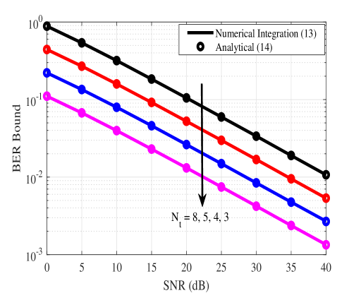
Figure 3: Comparion between the union bound on BER calculated from (8), obtained from simulated PEP from (13), and closed-form PEP (19), for different $N_{t}=8,5,4,3$, with $n_{t}=2$.

Figure 4: Comparison of spectral efficiencies of N-GSSK and iN-GSSK.

The spectral efficiency for the proposed N-GSSK, is compared with that of iN-GSSK in Fig. 4. It is recalled here that in an iN-GSSK system, GSSK users are assumed to have the perfect knowledge of NOMA signals, which is unrealistic, particularly in practical scenarios. Although, at low SNR values, the spectral efficiency of the proposed N-GSSK is lower than that of iN-GSSK, it can be observed that both schemes demonstrate similar performance at moderate-to-high SNR. Note that the performance loss of the N-GSSK is due to the suboptimality of energy-based ML detector. Furthermore, as shown, the spectral efficiency of the N-GSSK increases with increasing $N_{t}$ for a given $n_{t}$.

Figure 5: Comparison of spectral efficiencies of N-GSSK, c-GSSK and c-NOMA for two and three users scenarios, with $N_{t}=5$ and $n_{t}=3$.

The spectral efficiency of N-GSSK, c-GSSK, and c-NOMA with $N_{t}=5$ and $n_{t}=3$ is presented in Fig. 5. The power allocation coefficients are chosen as follows. For the two user scenario, $\alpha_{1}=0.8$, and $\alpha_{2}=0.2$, while for the three user scenario, $\alpha_{1}=0.7$, $\alpha_{2}=0.2$, and $\alpha_{3}=0.1$. It can be observed that N-GSSK yields a better spectral efficiency compared to c-GSSK, which further increases as the number of NOMA users increases. Additionally, the proposed N-GSSK yields a better spectral efficiency compared to c-NOMA, as it exploits the capacity gains due to both spatial and power domain multiplexing.

Figure 6: Comparison of spectral efficiencies of N-GSSK (for $n_{t}$=2) and N-SSK (for $n_{t}=1$) for different $N_{t}$.

Finally, Fig. 6 demonstrate the impact of the number of transmit antennas on the spectral efficiency of N-GSSK. As mentioned earlier, N-SSK is a special case of N-GSSK, where $n_{t}=1$. For illustration purposes, we choose $n_{t}=2$ for N-GSSK. When $N_{t}=2$, the performances of N-GSSK and N-SSK are equal, since the number of possible antenna indices are equal in both cases. As expected, N-GSSK outperforms N-SSK as $N_{t}$ increases.

VI Conclusion

In this paper, we analyzed the spectral efficiency of N-GSSK and proposed a novel, energy-based maximum likelihood detection scheme for N-GSSK. Unlike [37], GSSK users in our setup can estimate active antenna indices without the knowledge of NOMA signals. By transmitting the superimposed NOMA signals and active antenna indices, we demonstrate that the spectral efficiency can be further enhanced. Furthermore, we investigated the performance of the proposed energy-based ML detector through the derivation of closed-form expressions for the pairwise error probability and BER union bound. Monte Carlo simulations and numerical results were presented in order to corroborate the analysis and establish the accuracy of derived expressions. Finally, we demonstrated that the N-GSSK scheme achieves significant spectral efficiency improvement, as opposed to the c-GSSK.

VII Appendix: Proof of Proposition 1

Let us define $x\triangleq\frac{\xi}{n_{t}}$, and $y\triangleq\frac{\zeta}{n_{t}}$ in (13). Therefore

$$P(x_{j}\rightarrow x_{k})=\int_{0}^{\infty}\int_{0}^{\infty}Q\left(a\left|x-y\right|\right)e^{-x}e^{-y}dxdy.$$ (34)

Noting that

$$Q(|z|)=\frac{1}{2}\left[1-\text{erf}\left(\frac{|z|}{\sqrt{2}}\right)\right],$$ (35)

the above integral can be written as

$$P(x_{j}\rightarrow x_{k})=\frac{1}{2}\left[\underset{\triangleq\mathcal{I}_{1}}{\underbrace{\int_{0}^{\infty}e^{-x}dx\int_{0}^{\infty}e^{-y}dy}}\right.$$

$$\leavevmode\nobreak\ \leavevmode\nobreak\ \leavevmode\nobreak\ \leavevmode\nobreak\ \leavevmode\nobreak\ \leavevmode\nobreak\ \leavevmode\nobreak\ \leavevmode\nobreak\ \leavevmode\nobreak\ \leavevmode\nobreak\ \leavevmode\nobreak\ \leavevmode\nobreak\ \leavevmode\nobreak\ \leavevmode\nobreak\ \left.-\underset{\triangleq\mathcal{I}_{2}}{\underbrace{\int_{0}^{\infty}e^{-x}dx\int_{0}^{\infty}\text{erf}\left(\gamma\left|x-y\right|\right)e^{-y}dy}}\right],$$ (36)

where $\gamma=a/\sqrt{2}$. It is easy to see that $\mathcal{I}_{1}=1$. Also,

$$\mathcal{I}_{2}=\frac{1}{\sqrt{\pi}2\pi j}\oint_{\mathcal{C_{\textrm{s}}}}\frac{\Gamma(s)\Gamma\left(\frac{1}{2}-s\right)}{\Gamma\left(\frac{3}{2}-s\right)}\gamma^{-2s+1}ds$$

$$\leavevmode\nobreak\ \leavevmode\nobreak\ \leavevmode\nobreak\ \leavevmode\nobreak\ \leavevmode\nobreak\ \leavevmode\nobreak\ \leavevmode\nobreak\ \leavevmode\nobreak\ \leavevmode\nobreak\ \leavevmode\nobreak\ \leavevmode\nobreak\ \leavevmode\nobreak\ \leavevmode\nobreak\ \leavevmode\nobreak\ \left[\int_{0}^{\infty}e^{-x}dx\int_{0}^{\infty}e^{-y}\left|x-y\right|^{-2s+1}dy\right],$$ (37)

where $\mathcal{C_{\textrm{s}}}$ is an appropriately chosen complex contour, ensuring the convergence of the above Mellin-Barnes integral. Substituting $z=\frac{y}{x}$, and further simplification yields (40).

$$\mathcal{I}_{2}=\frac{1}{2\sqrt{\pi^{3}}j}\oint_{\mathcal{C_{\textrm{s}}}}\frac{\Gamma(s)\Gamma\left(\frac{1}{2}-s\right)}{\Gamma\left(\frac{3}{2}-s\right)}\gamma^{-2s+1}ds\int_{0}^{\infty}x^{-2s+2}e^{-x}dx\int_{0}^{\infty}e^{-zx}\left|1-z\right|^{-2s+1}dz$$

$$\phantom{\mathcal{I}_{2}}=\frac{1}{\sqrt{\pi}}\left[\begin{array}[]{c}\underset{\triangleq\mathcal{I}_{2}^{(1)}}{\underbrace{\frac{1}{2\pi j}\oint_{\mathcal{C_{\textrm{s}}}}\frac{\Gamma(s)\Gamma\left(\frac{1}{2}-s\right)}{\Gamma\left(\frac{3}{2}-s\right)}\gamma^{-2s+1}ds\underset{\triangleq\mathcal{J}_{2}}{\underbrace{\int_{0}^{1}\left(1-z\right)^{-2s+1}\underset{\triangleq\mathcal{J}_{1}}{\underbrace{\int_{0}^{\infty}x^{-2s+2}e^{-x(z+1)}dx}dz}}}}}\\ +\underset{\triangleq\mathcal{I}_{2}^{(2)}}{\underbrace{\frac{1}{2\pi j}\oint_{\mathcal{C_{\textrm{s}}}}\frac{\Gamma(s)\Gamma\left(\frac{1}{2}-s\right)}{\Gamma\left(\frac{3}{2}-s\right)}\gamma^{-2s+1}ds\underset{\triangleq\mathcal{J}_{4}}{\underbrace{\int_{0}^{\infty}x^{-2s+2}e^{-x}dx\underset{\triangleq\mathcal{J}_{3}}{\underbrace{\int_{1}^{\infty}\left(z-1\right)^{-2s+1}e^{-xz}}dz}}}}}\end{array}\right]$$ (40)

Using [45, Eqs. 3.381.4, 3.194.1] for simplification, we get

$$\mathcal{J}_{1}=\frac{\Gamma\left(-2s+3\right)}{(z+1)^{-2s+3}},$$ (41)

$$\mathcal{J}_{2}=\Gamma\left(-2s+3\right)\int_{0}^{1}(z+1)^{2s-3}\left(1-z\right)^{-2s+1}dz$$

$$\phantom{\mathcal{J}_{2}}=2^{2s-3}\Gamma\left(-2s+3\right)\int_{0}^{1}u^{-2s+1}\left(1-\frac{u}{2}\right){}^{2s-3}du$$

$$\phantom{\mathcal{J}_{2}}={\frac{2^{2s-3}\Gamma\left(-2s+3\right)}{-2s+2}}$$

$$\leavevmode\nobreak\ \leavevmode\nobreak\ \leavevmode\nobreak\ \leavevmode\nobreak\ \leavevmode\nobreak\ \leavevmode\nobreak\ \leavevmode\nobreak\ \leavevmode\nobreak\ \leavevmode\nobreak\ \leavevmode\nobreak\ \leavevmode\nobreak\ \times\text{ }_{2}F_{1}\left(-2s+3,-2s+2;-2s+3;\frac{1}{2}\right)$$

$$\phantom{\mathcal{J}_{2}}=2^{2s-3}\Gamma\left(-2s+2\right)\text{ }_{1}F_{0}\left(-2s+2;\cdot;\frac{1}{2}\right),$$ (42)

where ${}_{p}F_{q}(\cdot)$ is the hypergeometric function [45]. Substituting (41) and (42) into (40) and simplifying further gives

$$\mathcal{I}_{2}^{(1)}=\frac{1}{2\pi j}\oint_{\mathcal{C_{\textrm{s}}}}\frac{\Gamma(s)\Gamma\left(\frac{1}{2}-s\right)\Gamma\left(-2s+2\right)2^{2s-3}}{\Gamma\left(\frac{3}{2}-s\right)}$$

$$\leavevmode\nobreak\ \leavevmode\nobreak\ \leavevmode\nobreak\ \leavevmode\nobreak\ \leavevmode\nobreak\ \leavevmode\nobreak\ \leavevmode\nobreak\ \leavevmode\nobreak\ \leavevmode\nobreak\ \leavevmode\nobreak\ \leavevmode\nobreak\ \leavevmode\nobreak\ \leavevmode\nobreak\ \leavevmode\nobreak\ \leavevmode\nobreak\ \leavevmode\nobreak\ \times\gamma^{-2s+1}\text{ }_{1}F_{0}\left(-2s+2;.;\frac{1}{2}\right)ds$$

$$\phantom{\mathcal{I}_{2}^{(1)}}=\frac{\gamma}{4\sqrt{\pi}}\sum_{k=0}^{\infty}\frac{1}{k!}\frac{1}{2\pi j}\times$$

$$\leavevmode\nobreak\ \leavevmode\nobreak\ \oint_{\mathcal{C_{\textrm{s}}}}\frac{\Gamma(s)\Gamma\left(\frac{1}{2}-s\right)\Gamma\left(1+\frac{k}{2}-s\right)\Gamma\left(\frac{3}{2}+\frac{k}{2}-s\right)}{\Gamma\left(\frac{3}{2}-s\right)}\gamma^{-2s}ds$$

$$\phantom{\mathcal{I}_{2}^{(1)}}=\frac{\gamma}{4\sqrt{\pi}}\sum_{k=0}^{\infty}\frac{1}{k!}G_{3,2}^{1,3}\left(\gamma^{2}\left|\begin{array}[]{c}\frac{1}{2},-\frac{k}{2},-\frac{1}{2}-\frac{k}{2};-\\ 0;-\frac{1}{2}\end{array}\right.\right).$$ (45)

Similarly, using [45, Eqs. 3.381.2], it can be shown that

$$\mathcal{J}_{3}=x^{2s-2}e^{-x}\Gamma\left(-2s+2\right),$$ (46)

$$\mathcal{J}_{4}=\frac{\Gamma\left(-2s+2\right)}{2}.$$ (47)

Substituting (46) and (47) into (40) gives

$$\mathcal{I}_{2}^{(2)} =\frac{\gamma}{\sqrt{\pi}}\frac{1}{2\pi j}\oint_{\mathcal{C_{\textrm{s}}}}\Gamma(s)\Gamma\left(\frac{1}{2}-s\right)\Gamma\left(1-s\right)\left(2\gamma\right)^{-2s}ds$$

$$=\frac{\gamma}{\sqrt{\pi}}G_{2,2}^{1,2}\left(\left(2\gamma\right)^{2}\left|\begin{array}[]{c}\frac{1}{2},0;-\\ 0;-\frac{1}{2}\end{array}\right.\right).$$ (50)

Finally, substituting (50) and (45) into (40) and (36), and substituting for $a=\sqrt{2}\gamma$ yields (19).

References

- [1] X. Liu, Y. Liu, X. Wang, and H. Lin, “Highly efficient 3-D resource allocation techniques in 5G for NOMA-enabled massive MIMO and relaying systems,” IEEE J. Sel. Areas Commun., vol. 35, no. 12, pp. 2785–2797, Dec. 2017.
- [2] S. Silva, G. A. A. Baduge, M. Ardakani, and C. Tellambura, “NOMA-aided multi-way massive MIMO relaying,” IEEE Trans. Commun., vol. 68, no. 7, pp. 4050–4062, Jul. 2020.
- [3] W. Shao, S. Zhang, H. Li, N. Zhao, and O. A. Dobre, “Angle-domain NOMA over multicell millimeter wave massive MIMO networks,” IEEE Trans. Commun., vol. 68, no. 4, pp. 2277–2292, Apr. 2020.
- [4] T. S. Rappaport, Y. Xing, G. R. MacCartney, A. F. Molisch, E. Mellios, and J. Zhang, “Overview of millimeter wave communications for fifth-generation (5G) wireless networks—with a focus on propagation models,” IEEE Trans. Antennas Propag., vol. 65, no. 12, pp. 6213–6230, Dec. 2017.
- [5] T. S. Rappaport, S. Sun, R. Mayzus, H. Zhao, Y. Azar, K. Wang, G. N. Wong, J. K. Schulz, M. Samimi, and F. Gutierrez, “Millimeter wave mobile communications for 5G cellular: It will work!” IEEE Access, vol. 1, pp. 335–349, May 2013.
- [6] F. Al-Ogaili and R. M. Shubair, “Millimeter-wave mobile communications for 5G: challenges and opportunities,” in Proc. IEEE International Symposium on Antennas and Propagation (APSURSI), Jun. 2016, pp. 1003–1004.
- [7] D. K. Hendraningrat, G. B. Satrya, and I. N. A. Ramatryana, “Coordinated beamforming for multi-cell non-orthogonal multiple access-based spatial modulation,” IEEE Access, vol. 8, pp. 113 456–113 466, Jun. 2020.
- [8] R. Y. Mesleh, H. Haas, S. Sinanovic, C. W. Ahn, and S. Yun, “Spatial modulation,” IEEE Trans. Veh. Technol., vol. 57, no. 4, pp. 2228–2241, Jul. 2008.
- [9] J. Jeganathan, A. Ghrayeb, L. Szczecinski, and A. Ceron, “Space shift keying modulation for MIMO channels,” IEEE Trans. Wireless Commun., vol. 8, no. 7, pp. 3692–3703, Jul. 2009.
- [10] M. D. Renzo and H. Haas, “Bit error probability of space-shift keying MIMO over multiple-access independent fading channels,” IEEE Trans. Veh. Technol., vol. 60, no. 8, pp. 3694–3711, Oct. 2011.
- [11] S. M. R. Islam, N. Avazov, O. A. Dobre, and K. Kwak, “Power-domain non-orthogonal multiple access (NOMA) in 5G systems: Potentials and challenges,” IEEE Commun. Surveys Tuts., vol. 19, no. 2, pp. 721–742, Secondquarter 2017.
- [12] M. T. P. Le, G. C. Ferrante, G. Caso, L. De Nardis, and M. Di Benedetto, “On information-theoretic limits of code-domain NOMA for 5G,” IET Commun., vol. 12, no. 15, pp. 1864–1871, Sep. 2018.
- [13] D. Wan, M. Wen, F. Ji, H. Yu, and F. Chen, “Non-orthogonal multiple access for cooperative communications: Challenges, opportunities, and trends,” IEEE Wireless Commun., vol. 25, no. 2, pp. 109–117, Apr. 2018.
- [14] J. Jeganathan, A. Ghrayeb, and L. Szczecinski, “Spatial modulation: optimal detection and performance analysis,” IEEE Commun. Lett., vol. 12, no. 8, pp. 545–547, Aug. 2008.
- [15] J. Jeganathan, A. Ghrayeb, L. Szczecinski, and A. Ceron, “Space shift keying modulation for MIMO channels,” IEEE Trans. Wireless Commun., vol. 8, no. 7, pp. 3692–3703, Jul. 2009.
- [16] J. Jeganathan, A. Ghrayeb, and L. Szczecinski, “Generalized space shift keying modulation for MIMO channels,” in Proc. IEEE 19th International Symposium on Personal, Indoor and Mobile Radio Communications, Sep. 2008, pp. 1–5.
- [17] S. Su, W. Chung, and C. Wu, “Exploiting entire GSSK antenna combinations in MIMO systems,” IEEE Commun. Lett., vol. 19, no. 5, pp. 719–722, May 2015.
- [18] J. Kim and I. Lee, “Capacity analysis of cooperative relaying systems using non-orthogonal multiple access,” IEEE Commun. Lett., vol. 19, no. 11, pp. 1949–1952, Nov. 2015.
- [19] Z. Ding, M. Peng, and H. V. Poor, “Cooperative non-orthogonal multiple access in 5G systems,” IEEE Commun. Lett., vol. 19, no. 8, pp. 1462–1465, Aug. 2015.
- [20] F. Kara and H. Kaya, “On the error performance of cooperative-NOMA with statistical CSIT,” IEEE Commun. Lett., vol. 23, no. 1, pp. 128–131, Jan. 2019.
- [21] Z. Ding, H. Dai, and H. V. Poor, “Relay selection for cooperative NOMA,” IEEE Wireless Commun. Lett., vol. 5, no. 4, pp. 416–419, Aug. 2016.
- [22] Y. Liu, Z. Ding, M. Elkashlan, and H. V. Poor, “Cooperative non-orthogonal multiple access with simultaneous wireless information and power transfer,” IEEE J. Sel. Areas Commun., vol. 34, no. 4, pp. 938–953, Apr. 2016.
- [23] Q. Sun, S. Han, C. I, and Z. Pan, “On the ergodic capacity of MIMO NOMA systems,” IEEE Wireless Commun. Lett., vol. 4, no. 4, pp. 405–408, Aug. 2015.
- [24] F. Zhou, Y. Wu, Y. Liang, Z. Li, Y. Wang, and K. Wong, “State of the art, taxonomy, and open issues on cognitive radio networks with NOMA,” IEEE Wireless Commun., vol. 25, no. 2, pp. 100–108, Apr. 2018.
- [25] Y. Chen, L. Wang, Y. Ai, B. Jiao, and L. Hanzo, “Performance analysis of NOMA-SM in vehicle-to-vehicle massive MIMO channels,” IEEE J. Sel. Areas Commun., vol. 35, no. 12, pp. 2653–2666, Dec. 2017.
- [26] C. Liu and D. Liang, “Heterogeneous networks with power-domain NOMA: coverage, throughput, and power allocation analysis,” IEEE Trans. Wireless Commun., vol. 17, no. 5, pp. 3524–3539, May 2018.
- [27] M. S. Ali, H. Tabassum, and E. Hossain, “Dynamic user clustering and power allocation for uplink and downlink non-orthogonal multiple access (NOMA) systems,” IEEE Access, vol. 4, pp. 6325–6343, Aug. 2016.
- [28] H. Liu, Z. Ding, K. J. Kim, K. S. Kwak, and H. V. Poor, “Decode-and-forward relaying for cooperative NOMA systems with direct links,” IEEE Trans. Wireless Commun., vol. 17, no. 12, pp. 8077–8093, Dec. 2018.
- [29] Q. Wu, W. Chen, D. W. K. Ng, and R. Schober, “Spectral and energy-efficient wireless powered IoT networks: NOMA or TDMA?” IEEE Trans. Veh. Technol., vol. 67, no. 7, pp. 6663–6667, Jul. 2018.
- [30] M. Hedayati and I. Kim, “On the performance of NOMA in the two-user SWIPT system,” IEEE Trans. Veh. Technol., vol. 67, no. 11, pp. 11 258–11 263, Nov. 2018.
- [31] Z. Song, Q. Ni, and X. Sun, “Spectrum and energy efficient resource allocation with QoS requirements for hybrid MC-NOMA 5G systems,” IEEE Access, vol. 6, pp. 37 055–37 069, 2018.
- [32] R. F. Siregar, F. W. Murti, and S. Y. Shin, “Combination of spatial modulation and non-orthogonal multiple access using hybrid detection scheme,” in Proc. Ninth International Conference on Ubiquitous and Future Networks (ICUFN), Jul. 2017, pp. 476–481.
- [33] C. Zhong, X. Hu, X. Chen, D. W. K. Ng, and Z. Zhang, “Spatial modulation assisted multi-antenna non-orthogonal multiple access,” IEEE Wireless Communications, vol. 25, no. 2, pp. 61–67, Apr. 2018.
- [34] Q. Li, M. Wen, E. Basar, H. V. Poor, and F. Chen, “Spatial modulation-aided cooperative NOMA: Performance analysis and comparative study,” IEEE J. Sel. Areas Commun., vol. 13, no. 3, pp. 715–728, Jun. 2019.
- [35] X. Zhu, Z. Wang, and J. Cao, “NOMA-based spatial modulation,” IEEE Access, vol. 5, Mar. 2017.
- [36] M. Irfan, B. S. Kim, and S. Y. Shin, “A spectral efficient spatially modulated non-orthogonal multiple access for 5G,” in 2015 International Symposium on Intelligent Signal Processing and Communication Systems (ISPACS), Nov. 2015, pp. 625–628.
- [37] J. W. Kim, S. Y. Shin, and V. C. M. Leung, “Performance enhancement of downlink NOMA by combination with GSSK,” IEEE Commun. Lett., vol. 7, no. 5, pp. 860–863, Oct. 2018.
- [38] K. Ntontin, M. Di Renzo, A. Perez-Neira, and C. Verikoukis, “Adaptive generalized space shift keying (GSSK) modulation for MISO channels: A new method for high diversity and coding gains,” in Proc. IEEE Vehicular Technology Conference (VTC Fall), Sep. 2012, pp. 1–5.
- [39] L. Bariah, S. Muhaidat, and A. Al-Dweik, “Error probability analysis of non-orthogonal multiple access over Nakagami-m fading channels,” IEEE Trans. Commun., vol. 67, no. 2, pp. 1586–1599, Feb. 2019.
- [40] J. Proakis and M. Salehi, Digital Communications, 5th Edition, 5th ed. McGraw-Hill, Nov. 2007.
- [41] S. Su, W. Chung, and C. Wu, “Exploiting entire GSSK antenna combinations in MIMO systems,” IEEE Commun. Lett., vol. 19, no. 5, pp. 719–722, May 2015.
- [42] A. Younis, N. Serafimovski, R. Mesleh, and H. Haas, “Generalised spatial modulation,” in Proc. Conference Record of the Forty Fourth Asilomar Conference on Signals, Systems and Computers, Nov. 2010, pp. 1498–1502.
- [43] M. Zeng, A. Yadav, O. A. Dobre, G. I. Tsiropoulos, and H. V. Poor, “On the sum rate of MIMO-NOMA and MIMO-OMA systems,” IEEE Wireless Commun. Lett., vol. 6, no. 4, pp. 534–537, Aug. 2017.
- [44] L. Bariah, A. Al-Dweik, and S. Muhaidat, “On the performance of non-orthogonal multiple access systems with imperfect successive interference cancellation,” in 2018 IEEE International Conference on Communications Workshops (ICC Workshops), May 2018, pp. 1–6.
- [45] I. Gradshteyn and I. Ryzhik, Tables of Integrals, Series and Products, 7th ed. Academic Press, 2007.