Approximating the Operating Characteristics of Bayesian Uncertainty Directed Trial Designs

Abstract

Bayesian response adaptive clinical trials are currently evaluating experimental therapies for several diseases. Adaptive decisions, such as pre-planned variations of the randomization probabilities, attempt to accelerate the development of new treatments. The design of response adaptive trials, in most cases, requires time consuming simulation studies to describe operating characteristics, such as type I/II error rates, across plausible scenarios. We investigate large sample approximations of pivotal operating characteristics in Bayesian Uncertainty directed trial Designs (BUDs). A BUD trial utilizes an explicit metric $u$ to quantify the information accrued during the study on parameters of interest, for example the treatment effects. The randomization probabilities vary during time to minimize the uncertainty summary $u$ at completion of the study.

We provide an asymptotic analysis (i) of the allocation of patients to treatment arms and (ii) of the randomization probabilities. For BUDs with outcome distributions belonging to the natural exponential family with quadratic variance function, we illustrate the asymptotic normality of the number of patients assigned to each arm and of the randomization probabilities. We use these results to approximate relevant operating characteristics such as the power of the BUD. We evaluate the accuracy of the approximations through simulations under several scenarios for binary, time-to-event and continuous outcome models.

Keywords: Adaptive Designs, Almost Sure Convergence, Bayesian Uncertainty Directed Trial Designs, Central Limit Theorem, Large Sample Approximations of Operating Characteristics, Stochastic Approximation

1 Introduction

Randomized clinical trials (RCTs) are essential to demonstrate the efficacy of novel experimental therapies [14]. The landscape of clinical studies has changed during the last decades, with an increasing number of trials that utilize adaptive designs, in some cases to evaluate several experimental treatments in biomarker-defined subpopulations [3, 33]. Adaptive designs are attractive to reduce the duration of the study and to allocate efficiently limited resources [8]. Most adaptive designs use data generated during the clinical trial for interim decisions [8], for example to vary the randomization probabilities during the study [3, 9, 33, 38] or to discontinue the evaluation of an experimental treatment [33]. In multi-arm studies adaptive randomization algorithms unbalance the randomization probabilities, in most cases, towards the most promising treatments. This can increase power compared to balanced randomization, and it can reduce the overall sample size necessary to test experimental treatments [35]. Adaptive randomization procedures have been developed for several designs, including multi-arm studies [9, 12], platform and basket studies [3, 33, 38].

The decision theoretic paradigm has been used to develop trial designs [7, 10, 16]. The study aims and costs are represented by a utility function $u(\cdot)$ of the data $\Sigma$ generated during the trial and the study design $d$. Using a Bayesian joint model for patient profiles, outcomes and other key variables, candidate designs $d$ can be compared by computing their expected utility $E[u(\Sigma,d)].$ The optimal design maximizes $E[u(\Sigma,d)]$ among all candidate designs. Several approximations of the described optimization have been proposed. For example, [34] discussed Bayesian Uncertainty directed trial Designs (BUDs), a class of approximate decision theoretic designs. The utility function $u$ in BUDs coincides with an information metric. In different words, the goal is to minimize uncertainty at completion of the study. BUDs for dose-finding and basket trials have been discussed in [17] and [31]. Previous work, related to BUDs, proposed information-based sampling schemes [11, 28, 30].

There is a rich literature on large sample analyses of adaptive designs. For instance, [1, 36] studied the behavior of sequential urn schemes. See also [2, 19, 29, 37] for a recent summary on large sample results for urn schemes. The limiting behavior of adaptive biased coin designs have been investigated, among others, by [18, 21] and [22]. Relevant work connecting stochastic approximation with response-adaptive clinical trials include [4] and [25].

In this manuscript we focus on the asymptotic characteristics of BUDs. The design of adaptive clinical trials requires the estimation of pivotal operating characteristics, such as type I and II error rates and the distribution of patients randomized to each treatment arm. In most cases these estimates are based on time consuming Monte Carlo simulations, conducted for different candidate designs and varying key parameters, including sample sizes, enrollment rates, and outcome distributions. Approximations of the operating characteristics, beyond simulations, using asymptotic results, are crucial to compare designs across plausible scenarios.

The need for computationally efficient approximations of design-specific operating characteristics motivates our study. We show the almost sure convergence and asymptotic normality of the relative allocation of patients to treatment arms in BUDs. We first derive analytic results assuming that the treatment-specific outcome distributions belong to natural exponential family [15], and later relax this assumption. In our analysis, we represent BUD randomization procedures as stochastic approximations (SAs). We study the ordinary differential equations associated with the resulting SAs and the stability of the stationary points, following the framework developed in [5] and using results of [24, 25]. We illustrate through examples the accuracy of the asymptotic approximations by comparing asymptotic and Monte-Carlo estimates of operating characteristics of BUDs.
Our asymptotic results allow investigators to quickly approximate the distribution of the number of patients that will be assigned to each arm and the power of BUDs.

2 Trial Design

We consider a clinical study that assigns $n$ patients sequentially to $K$ arms. We use $A_{t}\in\mathcal{A}=\{0,\cdots,K-1\}$ to indicate the assignment of individual $t=1,\cdots,n$ to treatment arm $A_{t}$ and $Y_{t}\in\mathbb{R}$ is the response of individual $t$. We summarize the accumulated data up to enrollment $t$ by $\Sigma_{t}=\{\left(A_{\ell},Y_{\ell}\right);\ell\leq t\}$.

The BUD is defined by first specifying a Bayesian model. Outcomes are conditionally independent $Y_{t}\sim f_{\theta}(Y_{t}|A_{t})$ and $\theta\sim\pi(\theta)$ indicates the prior for the unknown parameter $\theta$. The function $u(\cdot)$ translates the posterior distribution $\pi(\theta|\Sigma_{t})$ into utilities, and we use it to quantify the information $u(\Sigma_{t})$ generated by the experiment up to stage $t$. Large values of $u(\Sigma_{t})$ correspond to low uncertainty levels. The utility $u(\cdot)$ in a BUD is a convex functional of the posterior distribution of $\theta$, for example $u(\Sigma_{t})=-\text{Var}(\theta|\Sigma_{t})$. By Jensen’s inequality, the information, on average, increases with each enrollment,

$$\Delta_{t}(a) :=E\left[u(\Sigma_{t+1})|A_{t+1}=a,\Sigma_{t}\right]-u(\Sigma_{t})\geq 0,$$ (1)

for every $a\in\mathcal{A}$. The myopic and non randomized policy $A_{t+1}=\mathop{\arg\max}_{a\in\mathcal{A}}\Delta_{t}(a),$ which is often inappropriate for clinical experiments [9], is relaxed in BUDs by a randomized version, with randomization probabilities

$$p_{t,a}:=p(A_{t+1}=a\mid\Sigma_{t})\propto\Delta_{t}(a)^{h},$$ (2)

where $h\geq 0$ is a tuning parameter. The randomization probabilities coincide with the myopic policy when $h\rightarrow\infty$, while with $h=0$ the randomization probabilities become identical across arms.

2.1 Outcome distributions within the natural exponential family

We will focus on outcome distributions $f_{\theta}$ in the natural exponential family (NEF) [6],

$$f_{\theta}(y|A_{t}=a)=f_{\psi_{a}}(y)\propto\exp\{y\psi_{a}-b(\psi_{a})\},$$ (3)

where $\psi_{a}\in\mathbb{R}$ is the canonical parameter and $b(\cdot)$ is the cumulant transform. We indicate the mean with $\theta_{a}=E_{\psi}[Y_{t}|A_{t}=a]=b^{\prime}(\psi_{a})$ and we use the equivalent parametrization $f_{\psi_{a}}$ and $f_{\theta_{a}}$ interchangeably. We use independent conjugate prior distributions [15] for $\psi_{a}$,

$$\pi(\psi_{a}\mid n_{0,a},y_{0,a})\propto\exp\{n_{0,a}\tilde{y}_{0,a}\psi_{a}-n_{0,a}b(\psi_{a})\},$$ (4)

with hyper-parameters $n_{0,a}>0$ and $\tilde{y}_{0,a}\in\mathbb{R}$. The posterior distribution for $\psi=(\psi_{0},\cdots,\psi_{K-1})$ is $\pi(\psi\mid\Sigma_{t})=\prod_{a=0}^{K-1}\pi(\psi_{a}\mid\Sigma_{t})$, where $\pi(\psi_{a}\mid\Sigma_{t})$ has the same form as (4) with updated parameters $n_{t,a}=n_{0,a}+t\hat{p}_{t,a}$ and $\tilde{y}_{t,a}=\big{(}n_{0,a}\tilde{y}_{0,a}+\sum_{s=1}^{t}Y_{s}1{(A_{s}=a)}\big{)}\big{/}n_{t,a}$. Here $\hat{p}_{t,a}$ is the proportion of patients assigned to treatment $a$ by time $t$ and $1(A_{s}=a)=1$ if patient $s$ received treatment $a$ and zero otherwise. Let $\sigma_{a}^{2}=\int y^{2}f_{\psi_{a}}(y)dy-\left(\int yf_{\psi_{a}}(y)dy\right)^{2}.$
We consider

$$u(\Sigma_{t})=-\sum_{a=0}^{K-1}\text{Var}(\theta_{a}|\Sigma_{t}),$$ (5)

and the expected information increment is

$$\Delta_{t}(a)=\text{Var}(\theta_{a}\mid\Sigma_{t})-E[\text{Var}(\theta_{a}\mid\Sigma_{t+1})\mid A_{t+1}=a,\Sigma_{t}].$$ (6)

We recall a useful result from the literature on conjugate Bayesian models [6, 15], $\tilde{y}_{t,a}=E(\theta_{a}\mid\Sigma_{t})$. Since $A_{t+1}$ and $\theta_{a}$ are conditionally independent, given $\Sigma_{t}$, the information gain equals

$$\Delta_{t}(a) =\text{Var}(E(\theta_{a}\mid\Sigma_{t+1})\mid A_{t+1}=a,\Sigma_{t})$$

$$=\text{Var}\left(\frac{n_{0,a}+\tilde{y}_{0,a}+\sum_{s=1}^{t+1}Y_{s}1(A_{s}=a)}{n_{0,a}+t\hat{p}_{t,a}+1}\mid A_{t+1}=a,\Sigma_{t}\right)$$

$$=\text{Var}\left(\frac{Y_{t+1}}{n_{0,a}+t\hat{p}_{t,a}+1}\mid A_{t+1}=a,\Sigma_{t}\right),$$

where the first equality follows from the law of total variance. We can therefore write

$$\Delta_{t}(a)=\frac{\sigma_{t,a}^{2}}{(n_{0,a}+t\hat{p}_{t,a}+1)^{2}},$$

where $\sigma_{t,a}^{2}=\text{Var}(Y_{t+1}\mid A_{t+1}=a,\Sigma_{t})$.

3 Asymptotic properties

We discuss asymptotic properties of BUDs with sum of the (negative) posterior variances of $\theta_{a},a=0,\dots,K-1$, as information measure $u(\Sigma_{t})$. In [34] a criterion is given for the allocation proportions to have a limit. Based on this result, we first prove convergence of allocation proportions and randomization probabilities under the assumption that the outcome distributions belong to the natural exponential family. We then investigate the rate of convergence of these quantities in the case $K=2$.

Proposition 1.

Consider a two arm BUD, $K=2$, with outcome distribution belonging to the NEF (3), conjugates prior (4) and information metric $u(\Sigma_{t})$ in (5). Then, as $t\rightarrow\infty,$
(i) the allocation of patients to treatments $a=0,1$ converges almost surely (a.s.),

$$\widehat{p}_{t,a}\longrightarrow\rho_{a}:=\frac{\sigma_{a}^{\frac{2h}{2h+1}}}{\sigma_{0}^{\frac{2h}{2h+1}}+\sigma_{1}^{\frac{2h}{2h+1}}}\,\,\text{a.s. as }\small t\rightarrow\infty$$ (7)

(ii) the randomization probability converges a.s. to the same limit,

$$p_{t,a}\longrightarrow\rho_{a}\,\,\text{a.s. as }\small t\rightarrow\infty.$$ (8)

The proofs of the proposition and of all subsequent results are included in the Supplementary material. The following corollary states the extension of Proposition 1 for multi-arm settings $K>2$.

Corollary 1.

Under the same assumptions of Proposition 1, if $K>2$, then, as $t\rightarrow\infty,$ the allocation of patients to treatments $(\widehat{p}_{t,0},\dots,\widehat{p}_{t,K-1})$ and the randomization probabilities $({p}_{t,0},\dots,{p}_{t,K-1})$ converge a.s. to $(\rho_{0},\dots,\rho_{K-1})$, where for $a\in\{0,\dots,K-1\}$

$$\rho_{a}=\dfrac{\sigma_{a}^{\frac{2h}{2h+1}}}{\sum_{i=0}^{K-1}\sigma_{i}^{\frac{2h}{2h+1}}}.$$ (9)

We recall that the NEFs with quadratic variance function consist of all NEFs such that $\sigma^{2}_{a}=v_{0}+v_{1}\theta_{a}+v_{2}\theta_{a}^{2}$ for some constants $v_{0},v_{1},v_{2}$. In different words, the variance is a polynomial function of order $\leq 2$ of the mean [26]. This class contains models, such as the normal, Poisson, gamma, negative binomial and binomial distributions. We refer to Morris [26, 27] for a detailed study of this class of distributions.

We derive the rate of convergence and show the asymptotic normality of the randomization probabilities $p_{t,a}$ and of the allocation proportions $\widehat{p}_{t,a}$ in BUDs with utility $u(\Sigma_{t})=-\sum_{a=0}^{K-1}\text{Var}(\theta_{a}|\Sigma_{t})$ when $K$ equals $2$ and the model $f_{\theta_{a}}$ belongs to the NEF with quadratic variance. Lemma 1 approximates, for $a\in\{0,1\}$, the variables $\sigma_{t,a}$ and $\tilde{y}_{t+1,a}$ with functions of $(\tilde{y}_{t,a},p_{t,1})$ and $(Y_{t+1},A_{t+1})$. For $a=0,1,$ we use the following notation:

$$\Delta\sigma^{2}_{t,a}=\text{Var}(Y_{t+2}\mid A_{t+2}=a,\Sigma_{t+1})-\text{Var}(Y_{t+1}\mid A_{t+1}=a,\Sigma_{t}),$$

$v(\tilde{y}_{t,a})=\left(v_{0}+v_{1}\tilde{y}_{t,a}+v_{2}\tilde{y}_{t,a}^{2}\right)^{\frac{1}{2}}$, $W_{t}=[p_{t,1},\tilde{y}_{t,1},\tilde{y}_{t,0}]^{\prime}\,$ and $\,k_{a}(W_{t})=\left[1+\left(\dfrac{p_{t,a}}{p_{t,1-a}}\right)^{\frac{1}{2h}}\dfrac{v(\tilde{y}_{t,1-a})}{v(\tilde{y}_{t,a})}\right].$
We also write $X(t)=\mathcal{O}_{P}(t^{-\alpha})$, for $\alpha>0$, if for all $\epsilon>0$ there exist finite $T,M>0$ such that $P(|X(t)|>Mt^{-\alpha})<\epsilon$ for all $t>T.$

Lemma 1.

If the outcome distributions $f_{\psi_{a}},a=0,1$, of the two-arm BUD belong to the NEF with quadratic variance function, then

• $\sigma_{t,a}=v(\tilde{y}_{t,a})+\mathcal{O}_{P}(t^{-1})$

• $\tilde{y}_{t+1,a}=\tilde{y}_{t,a}+(Y_{t+1}-\tilde{y}_{t,a})\dfrac{1(A_{t+1}=a)}{t}k_{a}(W_{t})+\mathcal{O}_{P}(t^{-2})$

• $\Delta\sigma_{t,a}^{2}=(v_{1}+2v_{2}\tilde{y}_{t,a})(Y_{t+1}-\tilde{y}_{t,a})\dfrac{1(A_{t+1}=a)}{t}k_{a}(W_{t})+\mathcal{O}_{P}(t^{-2}).$

In spirit to the previous result, the next Lemma illustrates that $p_{t+1,1}$ can be approximated by a function of $W_{t},Y_{t+1},A_{t+1}$ with an $\mathcal{O}_{P}(t^{-2})$ error term.

Lemma 2.

Let the outcome distributions $f_{\psi_{a}},a=0,1$ of the two-arm BUD belong to the NEF with quadratic variance function. For the randomization probabilities $p_{t,1},t\geq 1$ it holds that

$$p_{t+1,1}=p_{t,1}+hp_{t,1}(1-p_{t,1})\Bigg{\{} \left[\dfrac{(v_{1}+2v_{2}\tilde{y}_{t,1})(Y_{t+1}-\tilde{y}_{t,1})}{v(\tilde{y}_{t,1})^{2}}-2\right]\dfrac{A_{t+1}}{t}k_{1}(W_{t})$$

$$+\! \left[2-\dfrac{(v_{1}+2v_{2}\tilde{y}_{t,0})(Y_{t+1}-\tilde{y}_{t,0})}{v(\tilde{y}_{t,0})^{2}}\right]\dfrac{(1-A_{t+1})}{t}k_{0}(W_{t})\Bigg{\}}+\mathcal{O}_{P}(t^{-2}).$$ (10)

The two Lemmas above suggest how to approximate $\tilde{y}_{t+1,a}-\tilde{y}_{t,a}$ for $a\in\{0,1\}$ and $p_{t+1,1}-p_{t,1}$. For $t\geq 1$, we define the random vector $\tilde{G}_{t+1}=[G_{t+1},G_{t+1,1},G_{t+1,0}]^{\prime}$, whose components are approximations of $t(p_{t+1,1}-p_{t,1})$ and $t(\tilde{y}_{t+1,a}-\tilde{y}_{t,a})$, respectively, where

$$G_{t+1}:=hp_{t,1}(1-p_{t,1})\Bigg{\{} \left[\dfrac{(v_{1}+2v_{2}\tilde{y}_{t,1})(Y_{t+1}-\tilde{y}_{t,1})}{v(\tilde{y}_{t,1})^{2}}-2\right]A_{t+1}k_{1}(W_{t})+$$

$$+\! \left[2-\dfrac{(v_{1}+2v_{2}\tilde{y}_{t,0})(Y_{t+1}-\tilde{y}_{t,0})}{v(\tilde{y}_{t,0})^{2}}\right](1-A_{t+1})k_{0}(W_{t})\Bigg{\}},$$

and $G_{t+1,a}:=1(A_{t+1}=a)(Y_{t+1}-\tilde{y}_{t,a})k_{a}(W_{t})$ for $a=0,1$. By computing the conditional expectations $\tilde{g}(W_{t})=-E_{\psi}(\tilde{G}_{t+1}\mid\Sigma_{t})$ we define the map $\tilde{g}(\cdot)=[g(\cdot),g_{1}(\cdot),g_{0}(\cdot)]^{\prime}$, whose components are

$$g(W_{t}) :=-{2h}\dfrac{v(\tilde{y}_{t,1})}{v(\tilde{y}_{t,0})}\dfrac{(1-p_{t,1})^{\frac{2h+1}{2h}}}{p_{t,1}^{\frac{1-2h}{2h}}}k_{1}(W_{t})^{2}\left(\dfrac{1}{k_{1}(W_{t})}-p_{t,1}\right)-hp_{t,1}(1-p_{t,1})\times$$

$$\left[p_{t,1}\dfrac{(v_{1}+2v_{2}\tilde{y}_{t,1})(b^{\prime}(\psi_{1})-\tilde{y}_{t,1})}{v(\tilde{y}_{t,1})^{2}}k_{1}(W_{t})-(1-p_{t,1})\dfrac{(v_{1}+2v_{2}\tilde{y}_{t,0})(b^{\prime}(\psi_{0})-\tilde{y}_{t,0})}{v(\tilde{y}_{t,0})^{2}}k_{0}(W_{t})\right],$$

$$g_{a}(W_{t}) :=-p_{t,a}(b^{\prime}(\psi_{a})-\tilde{y}_{t,a})k_{a}(W_{t})\quad\text{for }a\in\{0,1\}.$$

In Proposition 2 we rewrite $t(W_{t+1}-W_{t})$ as the sum of (i) a function of $W_{t}$, (ii) a $\Sigma_{t}$ -martingale-difference sequence $\Delta\tilde{M}_{t+1}$ and (iii) a $\Sigma_{t+1}$-measurable sequence of remainder terms. In particular, $\Delta\tilde{M}_{t+1}=[\Delta M_{t+1},\Delta{M}_{t+1,1},\Delta{M}_{t+1,0}]^{\prime}$ is defined by $\tilde{G}_{t+1}+\tilde{g}(W_{t})$.

Proposition 2.

Let the outcome distributions $f_{\psi_{a}},a=0,1$, of the two-arm BUD, with information metric $u(\Sigma_{t})$ in (5), belong to the NEF with quadratic variance function. Then,

$$W_{t+1}=W_{t}-\dfrac{1}{t}\tilde{g}(W_{t})+\dfrac{1}{t}(\Delta\tilde{M}_{t+1}+\tilde{r}_{t+1}),$$ (11)

where the reminder terms $\tilde{r}_{t+1}:=[r_{t+1},r_{t+1,1},r_{t+1,0}]$ are three $\mathcal{O}_{P}(t^{-1})$ sequences.

Using Proposition 2 we use the theory of stochastic approximation [5, 24] to derive the asymptotic distribution of $W_{t}$. Following the stochastic approximation framework, we consider equation (11) together with the ordinary differential equation (ODE)

$$\frac{dW_{t}}{dt}=-\tilde{g}(W_{t}),$$ (12)

where $t\in(0,+\infty)$ denotes continuous time. The ODE has arbitrary initial conditions. Note that if we ignore the residual term $\tilde{r}_{t+1}$, the difference $W_{t+1}-W_{t}$ in (11) is equal to $-\frac{1}{t}\tilde{g}(W_{t})$ plus a $\Sigma_{t}$-martingale-difference sequence. We describe the distribution of $W_{t}$, for large $t$, using on an asymptotic analysis of the ODE (12). By identifying the stationary point $[\rho_{1},b^{\prime}(\psi_{1}),b^{\prime}(\psi_{0})]$ of the ODE, assessing its stability, and using some regularity conditions on $\Delta\tilde{M}_{t+1}$ and $\tilde{r}_{t+1}$, we prove a central limit type result for $W_{t}$. In particular, Theorem 1 indicates the asymptotic normality of the randomization probability $p_{t,1}$.

Theorem 1.

Under the assumptions of Proposition 2, $t^{1/2}(p_{t,1}-\rho_{1})\rightarrow\mathcal{N}\Big{(}0,\dfrac{\Gamma}{1+4h}\Big{)},$ as $t\rightarrow+\infty$, where

$$\Gamma=h^{2}\rho_{1}^{2}(1-\rho_{1})^{2}\left[\dfrac{(v_{1}+2v_{2}b^{\prime}(\psi_{1}))^{2}}{\rho_{1}\sigma_{1}^{2}}+\dfrac{(v_{1}+2v_{2}b^{\prime}(\psi_{0}))^{2}}{(1-\rho_{1})\sigma_{0}^{2}}+\dfrac{4}{\rho_{1}}+\dfrac{4}{1-\rho_{1}}\right].$$ (13)

The following corollary verifies the asymptotic normality of the relative allocation $\hat{p}_{t,1}$ by applying the Delta method and Slutsky’s Theorem.

Corollary 2.

Under the assumptions of Theorem 13, as $t\rightarrow+\infty$,

$$t^{1/2}(\hat{p}_{t,1}-\rho_{1})\longrightarrow\mathcal{N}\Big{(}0,\frac{\Gamma}{4h^{2}(1+4h)}+\dfrac{\rho_{1}(1-\rho_{1})^{2}}{4\sigma_{1}^{2}}(v_{1}+2v_{2}b^{\prime}(\psi_{1}))^{2}+\dfrac{\rho_{1}^{2}(1-\rho_{1})}{4\sigma_{0}^{2}}(v_{1}+2v_{2}b^{\prime}(\psi_{0}))^{2}\Big{)}.$$

4 Applications and examples

We apply the results in the previous section to the design of clinical trials. We consider three common outcomes, binary, time to event and continuous outcomes.

Binary outcomes. For $Y_{t}\in\{0,1\}$, we use the Bernoulli model $f_{\psi_{a}}(1)=1-f_{\psi_{a}}(0)=\theta_{a}$, $\theta_{a}=1/(1+e^{-\psi_{a}})$, and conjugated prior $\theta_{a}\sim\mbox{Beta}(\alpha,\beta).$ The outcome variance $\sigma^{2}_{a}$ in expression (7) is $\theta_{a}(1-\theta_{a})$, and the parameters of the quadratic variance function in (13) are $v_{1}=1$ and $v_{2}=-1$. Therefore, $t^{1/2}(\hat{p}_{t,1}-\rho_{1})$ converges in distribution to a mean zero Gaussian variable with variance

$$\dfrac{\rho_{1}^{2}(1-\rho_{1})^{2}}{4}\left[\left(\dfrac{(1-2\theta_{1})^{2}}{\rho_{1}\sigma_{1}^{2}}+\dfrac{(1-2\theta_{0})^{2}}{(1-\rho_{1})\sigma_{0}^{2}}\right)\left(1+\dfrac{1}{1+4h}\right)+\dfrac{4}{\rho_{1}(1+4h)}+\dfrac{4}{(1-\rho_{1})(1+4h)}\right].$$

The top panel of the second column of Figure 1 shows a trajectory $\hat{p}_{t,1},t=1,\cdots,10,000$ for a single simulated two-arm BUD trial (black curve). The response probabilities $(\theta_{0},\theta_{1})$ are set equal to $0.2$ and $0.4$. We used $\alpha=\beta=2$ and $h=5$. The shaded area shows (point-wise at each $t$) upper and lower 2.5% quantiles of the distribution of $\hat{p}_{t,1}$ across 1,000 simulations. The second row illustrates the distribution of $t^{1/2}(\hat{p}_{t,1}-\rho_{1})$ across 1000 simulations of the two-arm BUD trial. The empirical distribution of $t^{1/2}(\hat{p}_{t,1}-\rho_{1})$ has been smoothed with a kernel density estimator. The panel compares the $\mathcal{N}(0,0.097)$ density (asymptotic approximation) to the empirical distribution of $t^{1/2}(\hat{p}_{t,1}-\rho_{1})$ across simulations, when $t=100,1000$ and $10,000$. The last row compares the empirical distribution distribution of $t^{1/2}(p_{t,1}-\rho_{1})$ to the $\mathcal{N}\Big{(}0,\dfrac{\Gamma}{1+4h}\Big{)}$ density.

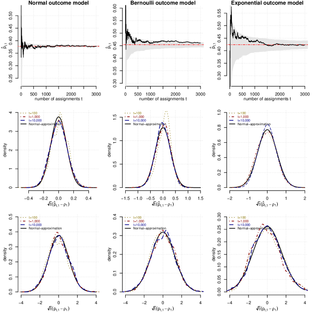
Figure 1: The panels in the first row compare $\hat{p}_{t,1}$ with the limit $\rho_{1}$ (red line) in each of the three examples (binary, continuous and time to event outcomes). The other panels compare asymptotic and empirical distributions of randomization probabilities $p_{t,1}$ and allocation proportions $\hat{p}_{t,1}$. The empirical distributions in each of the three examples (binary, continuous and time to event outcomes) are based on 1000 simulations of the two-arm BUD trial.

Time-to-event outcomes. We consider an exponential model $f_{\psi_{a}}(y)=\exp\{-y\psi_{a}\}\psi_{a},y\geq 0$ with mean $\theta_{0}=1/\psi_{a}$, and we use the conjugated gamma prior $\psi_{a}\sim\mbox{Gamma}(\alpha,\beta)$. The outcome variance $\sigma^{2}_{a}$ in expression (7) is $1/\psi_{a}^{2}$, the parameters of the quadratic variance function in (13) are $(v_{1},v_{2})=(0,1)$ and $h=5$. Therefore, the asymptotic variance of $t^{1/2}(\hat{p}_{t,1}-\rho_{1})$ is

$$\rho_{1}^{2}(1-\rho_{1})^{2}\left(\dfrac{1}{\rho_{1}}+\dfrac{1}{1-\rho_{1}}\right)\left(\dfrac{2}{1+4h}+1\right).$$

The third column of Figure 1 compares the asymptotic and empirical distributions of $t^{1/2}(\hat{p}_{t,1}-\rho_{1})$ and $t^{1/2}(p_{t,1}-\rho_{1})$, based on 1000 simulations of the BUD trial. In this example $(\theta_{0},\theta_{1})=(5,7)$ and $(\alpha,\beta)=(3,3).$

Continuous outcomes. We consider a normal outcome model $\mathcal{N}(\theta_{a},\sigma^{2}_{a})$ with known variance $\sigma^{2}_{a}$. We use a conjugated prior $\theta_{a}{\sim}\mathcal{N}(0,v^{2}_{0,a}).$ In this case $v_{1}=v_{2}=0$, $h=5$, and

$$t^{1/2}(\hat{p}_{t,1}-\rho_{1})\underset{{\small t\rightarrow\infty}}{\longrightarrow}\mathcal{N}(0,\dfrac{\rho_{1}(1-\rho_{1})}{1+4h}).$$ (14)

Column 1 of Figure 1 illustrates the empirical distribution of $t^{1/2}(\hat{p}_{t,1}-\rho_{1})$, $t=100,1000$ or $10000$, and the normal approximation.

Power analysis and sample size selection. We use the results in Section 3 to select the sample size of BUD studies accordingly to the targeted type I and II error rates. We approximate the power function of the BUD under fixed scenarios using Corollary 2.

We assume that the primary aim of the clinical trial is to test the one-sided null hypothesis $H_{0}:\theta_{0,1}=\theta_{0,0}$ against the alternative $H_{1}:\theta_{0,1}>\theta_{0,0}$. We verified (Supplementary material) that, under the sequential BUD design, the maximum-likelihood estimates (MLE) $\widehat{\theta}_{t,a}$ of the unknown true mean response $\theta_{0,a}$ to treatment $a=0,1$ within the NEF of outcome models have the same limiting distribution as the MLE of a study design with fixed arm-specific sample sizes, i.e.

$$t^{1/2}\begin{bmatrix}\hat{\theta}_{t,0}-\theta_{0,0}\vspace{0.15 cm}\\ \hat{\theta}_{t,1}-\theta_{0,1}\end{bmatrix}\underset{{\small t\rightarrow\infty}}{\longrightarrow}\mathcal{N}\left(\bm{0},Diag(\eta_{0,0},\eta_{0,1})\right),$$ (15)

where $\eta_{0,a}:=\left(\rho_{a}I_{\theta_{0,a}}\right)^{-1}$ and $I_{\theta_{0,a}}$ is the Fisher information of $f_{\theta_{0,a}}$.

We use a standard Wald-statistics, $Z_{a}=\dfrac{\sqrt{t}\times(\hat{\theta}_{t,1}-\hat{\theta}_{t,0})}{\sqrt{\widehat{\eta}_{t,a}+\widehat{\eta}_{t,1}}},$ where $\widehat{\eta}_{t,a}=1/(\widehat{\rho}_{a}\times I_{\widehat{\theta}_{t,a}})$, and the MLE $\widehat{\sigma}^{2}_{a}$ for $\widehat{\rho}_{a}=\rho_{a}(\widehat{\sigma}^{2}_{a})$ in (7) to test $H_{0}$. The power function of the BUD design is approximated by $\Phi\Big{(}z_{1-\alpha}-\dfrac{\sqrt{t}(\theta_{0,1}-\theta_{0,0})}{\sqrt{\eta_{0,1}+\eta_{0,0}}}\Big{)}$ where $\Phi(\cdot)$ is the cumulative distribution function of a standard normal random distribution and $\Phi(z_{1-\alpha})=1-\alpha.$ Therefore $\widehat{t}_{1-\alpha,1-\beta}=\dfrac{(z_{1-\alpha}-z_{1-\beta})^{2}(\eta_{0,0}+\eta_{0,1})}{(\theta_{0,1}-\theta_{0,0})^{2}}$ approximates the sample size of the BUD study to achieve a power equal to 1-$\beta$ and type I error rate $\alpha$.

Figure 2 compares, for three BUD designs (binary, time-to-event and continuous outcomes), power estimates based on asymptotic approximations (blue dotted lines) and on Monte Carlo simulations (1000 simulated trials, blue solid lines). The computational time for the simulation-based calculations is orders of magnitude larger than the normal approximation. We also show the empirical estimates of the type I error rates (brown solid lines) for the outlined asymptotic testing procedure with target type I error rate of $\alpha=0.05$ (brown dotted lines). For the normal outcome model, $\sigma^{2}_{0}=1,\sigma_{1}^{2}=3$, and $\theta_{0}=\theta_{1}=0$ (null scenario, brown lines) or $(\theta_{1},\theta_{2})=(0,1)$ (positive treatment effect, blue lines). Similarly, for the Bernoulli and Exponential models the parameter values $\theta$ that defined null (brown lines) and alternative scenarios (blue lines) are indicated in the panels of Fig 2.

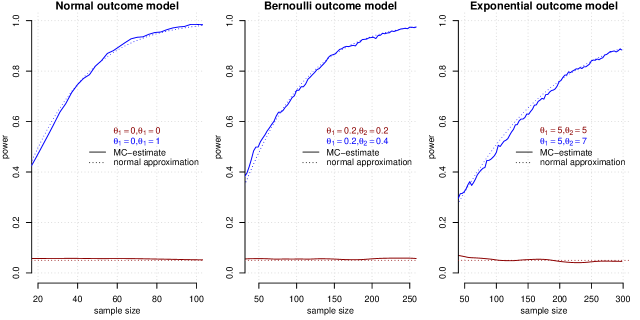
Figure 2: Power (blue lines) and type I error (red lines): comparison of estimates based on asymptotic approximations (dotted lines) and standard Monte Carlo simulations (1000 simulated trials, solid lines), for binary, continuous and time-to-event outcomes.

5 Convergence results beyond the NEF

We extend the almost sure convergence of the allocation proportion and randomization probability of a BUD (Proposition 1) to outcome distributions beyond the NEF. The following Lemma introduces approximations of the information increment (6) of BUDs with utility $u(\Sigma_{t})=-\sum_{a=0}^{1}\text{Var}(\theta_{a}|\Sigma_{t}),$ where $\theta_{a}$ is not required to be the mean of the outcomes as in Section 3. We use $X(t)=o_{P}(a(t))$ to indicate that $X(t)/a(t)$ converges to zero in probability.

Lemma 3.

Consider two-arm BUDs with information metric $u(\Sigma_{t})$ in (5). The parameter space $\Theta\subset\mathbb{R}$ is a bounded open interval, the parameter $\theta_{0,a}$ is an interior point of $\Theta$ for $a\in\{0,1\}$ and the prior is the uniform distribution on $\Theta$. If (i) $\inf_{y,\theta_{a}}f_{\theta_{a}}(y)>0$, (ii) $\sup_{y,\theta_{a}}f_{\theta_{a}}(y)<\infty$, and (iii) $\sup_{y,\theta_{a}}\bigg{|}\dfrac{\partial^{k}f_{\theta_{a}}(y)}{\partial\theta_{a}^{k}}\bigg{|}<\infty$ for $k=1,2,3,$ then

$$\Delta_{t}(a)=I_{\theta_{0,a}}^{-1}\times(t\hat{p}_{t,a})^{-2}+o_{P}((t\hat{p}_{t,a})^{-2}).$$ (16)

The following proposition states that, under the assumptions of Lemma 3, the asymptotic convergence (7) and (8) also hold outside the NEF.

Proposition 3.

Under the assumptions of Lemma 3, it holds that

$$\hat{p}_{t,a}\longrightarrow\rho_{a}:=\frac{I_{\theta_{0,a}}^{-\frac{h}{2h+1}}}{I_{\theta_{0,0}}^{-\frac{h}{2h+1}}+I_{\theta_{0,1}}^{-\frac{h}{2h+1}}}\,\,\text{a.s. as }\small t\rightarrow\infty.$$ (17)

and

$$p_{t,a}\longrightarrow\rho_{a}\,\,\text{a.s. as }\small t\rightarrow\infty.$$ (18)

for $a\in\{0,1\}$.

Note that assumption (i) of Lemma 3 implies that the support of the outcome distribution $f_{\theta_{a}}$ is bounded. The regularity conditions of Lemma 3 can be modified, for example to cover settings where the outcome support is unbounded. A list of alternative assumptions is specified in the Supplementary material.

To illustrate the result we consider as an outcome model $f_{\theta_{a}}$ beyond the NEF the truncated Weibull model $f_{\theta_{a}}(y)=\dfrac{e^{-(yr)^{\theta_{a}}}(ry)^{\theta_{a}-1}r\theta_{a}}{1-e^{-(t_{0}r)^{\theta_{a}}}}$, $y\in(0,t_{0})$, with unknown shape parameter $\theta_{a}$ and known rate $r$ parameter. Panels A and B of Figure 3 show, similar to Figure 1, a trajectory of $p_{t,1}$ (Panel A) and $\hat{p}_{t,1}$ (Panel B) $t=1,2\cdots,6000$ for a single simulated two-arm BUD trial with $r=1,\theta_{0}=1,\theta_{1}=1.5$ (black curve). The shaded area shows (point-wise at each $t$) upper and lower 2.5% quantiles of the empirical distribution of $p_{t,1}$ and $\hat{p}_{t,1}$ across 1,000 simulations. The blue lines indicate the means of $p_{t,1}$ and $\hat{p}_{t,1}$ across these simulations, while the red horizontal lines indicate their limit $\rho_{a}$.

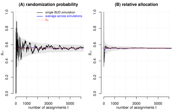
Figure 3: Allocation proportions and randomization probabilities of a two-arm BUD design. The primary outcomes are modeled with a truncated Weibull distribution. The average allocation proportion and randomization probability across 1000 simulations (blue lines) are close to their limit ($t\rightarrow\infty$, red lines).

6 Discussion

Asymptotic analyses of Bayesian adaptive procedures simplify the design of clinical trials and reduce the need for time-consuming simulations to evaluate operating characteristics across potential trial scenarios. We derived asymptotic results for the randomization probabilities and the allocation proportions of BUDs using stochastic approximation techniques. BUD’s randomization procedure was expressed as a sequence of recursive equations which allowed the application of techniques from classical stochastic approximation theory. This allowed us to derive a central limit theorem for the relative allocation of patients to treatments and for the randomization probabilities. Potential applications of stochastic approximation theory in the analysis of trial designs have been previously discussed by [25]. In our work we showed that they allow to evaluate major operating characteristics of BUDs. We considered for example the variability of the allocation proportions during the trials and the power of the BUD design with a fixed sample size under a parameter $\theta$ of interest. The stochastic approximation framework, as we showed in our examples, enables useful approximations of the patients’ assignment variability and other characteristics.

7 Supplementary Material: “Approximating the Operating Characteristics of Bayesian Uncertainty Directed Trial Designs”

Proof.

(Proposition 1) It is enough to prove (7) and (8) for $a=1$. First, define

$$F_{t}=-\hat{p}_{t,1}+\frac{\left(\frac{\sigma_{t,1}^{2}}{(t_{0}+t\hat{p}_{t,1}+1)^{2}}\right)^{h}}{\left(\frac{\sigma_{t,0}^{2}}{(t_{0}+t\hat{p}_{t,0}+1)^{2}}\right)^{h}+\left(\frac{\sigma_{t,1}^{2}}{(t_{0}+t\hat{p}_{t,1}+1)^{2}}\right)^{h}}$$

and

$$\tilde{F}_{t}=-\hat{p}_{t,1}+\frac{\hat{p}_{t,1}^{-2h}\sigma_{1}^{2h}}{\hat{p}_{t,0}^{-2h}\sigma_{0}^{2h}+\hat{p}_{t,1}^{-2h}\sigma_{1}^{2h}}.$$

As a function of $\hat{p}_{t,1}$, $\tilde{F}_{t}$ is strictly decreasing. The unique root of $\tilde{F}_{t}=0$ is

$$\rho_{1}:=\frac{\sigma_{1}^{2h/(2h+1)}}{\sigma_{0}^{2h/(2h+1)}+\sigma_{1}^{2h/(2h+1)}}$$ (19)

Now, we show that $F_{t}-\tilde{F}_{t}$ converges to zero a.s. as $t\rightarrow\infty$. The proof is based on the following elementary facts:

• If $a_{n}$, $b_{n}$, $a_{n}^{\prime}$ and $b_{n}^{\prime}$ are sequences of positive numbers, then

  $$\left|\frac{a_{n}}{a_{n}+b_{n}}-\frac{a_{n}^{\prime}}{a_{n}^{\prime}+b_{n}^{\prime}}\right|\leq\min\left(\left|\frac{a_{n}}{b_{n}}-\frac{a_{n}^{\prime}}{b_{n}^{\prime}}\right|,\left|\frac{b_{n}}{a_{n}}-\frac{b_{n}^{\prime}}{a_{n}^{\prime}}\right|\right)$$

  Indeed

  $$\left|\frac{a_{n}}{a_{n}+b_{n}}-\frac{a_{n}^{\prime}}{a_{n}^{\prime}+b_{n}^{\prime}}\right|=\left|\frac{1}{1+b_{n}/a_{n}}-\frac{1}{1+b_{n}^{\prime}/a_{n}^{\prime}}\right|=\left|\frac{b_{n}^{\prime}/a_{n}^{\prime}-b_{n}/a_{n}}{(1+b_{n}/a_{n})(1+b_{n}^{\prime}/a_{n}^{\prime})}\right|\leq\mid b_{n}^{\prime}/a_{n}^{\prime}-b_{n}/a_{n}\mid$$

  and

  $$\left|\frac{a_{n}}{a_{n}+b_{n}}-\frac{a_{n}^{\prime}}{a_{n}^{\prime}+b_{n}^{\prime}}\right|=\left|1-\frac{a_{n}}{a_{n}+b_{n}}-1+\frac{a_{n}^{\prime}}{a_{n}^{\prime}+b_{n}^{\prime}}\right|=\left|\frac{b_{n}}{a_{n}+b_{n}}-\frac{b_{n}^{\prime}}{a_{n}^{\prime}+b_{n}^{\prime}}\right|$$

• If $a_{n}$, $b_{n}$, $a_{n}^{\prime}$ and $b_{n}^{\prime}$ are bounded sequences of numbers such that $a_{n}-a_{n}^{\prime}\rightarrow 0$ and $b_{n}-b_{n}^{\prime}\rightarrow 0$, then $a_{n}b_{n}-a_{n}^{\prime}b_{n}^{\prime}\rightarrow 0$. Indeed,

  $$\mid a_{n}b_{n}-a_{n}^{\prime}b_{n}^{\prime}\mid\leq\mid a_{n}b_{n}-a_{n}^{\prime}b_{n}+a_{n}^{\prime}b_{n}-a_{n}^{\prime}b_{n}^{\prime}\mid\leq\mid b_{n}\mid\mid a_{n}-a_{n}^{\prime}\mid+\mid a_{n}^{\prime}\mid\mid b_{n}-b_{n}^{\prime}\mid$$

• If $a_{n}$ and $a_{n}^{\prime}$ are bounded sequences such that $a_{n}-a_{n}^{\prime}\rightarrow 0$ and $r$ is a positive real number, then $a_{n}^{r}-a_{n}^{\prime r}\rightarrow 0$. The thesis is obvious if $r=1$. If $r>1$, and $M$ is an upper bound for both sequences, then

  $$\mid a_{n}^{r}-a_{n}^{\prime r}\mid\leq 2rM^{r-1}\mid a_{n}-a_{n}^{\prime}\mid$$

  If $r<1$, then

  $$\mid a_{n}^{r}-a_{n}^{\prime r}\mid\leq\mid a_{n}-a_{n}^{\prime}\mid^{r}$$

Let us now prove that $F_{t}-\tilde{F}_{t}\rightarrow 0$ a.s.
By (a),

$$\mid F_{t}-\tilde{F}_{t}\mid\leq\min\left(\left|\frac{\sigma_{t,0}^{2h}((n_{0,1}+1)/t+\hat{p}_{t,1})^{2h}}{\sigma_{t,1}^{2h}((n_{0,0}+1)/t+\hat{p}_{t,0})^{2h}}-\frac{\sigma_{0}^{2h}\hat{p}_{t,1}^{2h}}{\sigma_{1}^{2h}\hat{p}_{t,0}^{2h}}\right|,\left|\frac{\sigma_{t,1}^{2h}((n_{0,0}+1)/t+\hat{p}_{t,0})^{2h}}{\sigma_{t,0}^{2h}((n_{0,1}+1)/t+\hat{p}_{t,1})^{2h}}-\frac{\sigma_{1}^{2h}\hat{p}_{t,0}^{2h}}{\sigma_{0}^{2h}\hat{p}_{t,1}^{2h}}\right|\right)$$

Hence

$$\mid F_{t}-\tilde{F}_{t}\mid \leq\left|\frac{\sigma_{t,0}^{2h}((n_{0,1}+1)/t+\hat{p}_{t,1})^{2h}}{\sigma_{t,1}^{2h}((n_{0,0}+1)/t+\hat{p}_{t,0})^{2h}}-\frac{\sigma_{0}^{2h}\hat{p}_{t,1}^{2h}}{\sigma_{1}^{2h}\hat{p}_{t,0}^{2h}}\right|1_{(\hat{p}_{t,0}>1/2)}+\left|\frac{\sigma_{t,1}^{2h}((n_{0,0}+1)/t+\hat{p}_{t,0})^{2h}}{\sigma_{t,0}^{2h}((n_{0,1}+1)/t+\hat{p}_{t,1})^{2h}}-\frac{\sigma_{1}^{2h}\hat{p}_{t,0}^{2h}}{\sigma_{0}^{2h}\hat{p}_{t,1}^{2h}}\right|1_{(\hat{p}_{t,0}\leq 1/2)}$$

$$\leq\left|\frac{\sigma_{t,0}^{2h}\sigma_{1}^{2h}((n_{0,1}+1)/t+\hat{p}_{t,1})^{2h}\hat{p}_{t,0}^{2h}-\sigma_{0}^{2h}\sigma_{t,1}^{2h}((n_{0,0}+1)/t+\hat{p}_{t,0})^{2h}\hat{p}_{t,1}^{2h}}{\sigma_{t,1}^{2h}\sigma_{1}^{2h}((n_{0,0}+1)/t+\hat{p}_{t,0})^{2h}\hat{p}_{t,0}^{2h}}\right|1_{(\hat{p}_{t,0}>1/2)}$$

$$+\left|\frac{\sigma_{t,1}^{2h}\sigma_{0}^{2h}((n_{0,0}+1)/t+\hat{p}_{t,0})^{2h}\hat{p}_{t,1}^{2h}-\sigma_{1}^{2h}\sigma_{t,0}^{2h}((n_{0,1}+1)/t+\hat{p}_{t,1})^{2h}\hat{p}_{t,0}^{2h}}{\sigma_{t,0}^{2h}\sigma_{0}^{2h}((n_{0,1}+1)/t+\hat{p}_{t,1})^{2h}\hat{p}_{t,1}^{2h}}\right|1_{(\hat{p}_{t,1}\geq 1/2)}$$

Thus,

$$\mid F_{t}-\tilde{F}_{t}\mid \leq\sigma_{t,1}^{-2h}\sigma_{1}^{-2h}2^{4h}\mid\sigma_{t,0}^{2h}\sigma_{1}^{2h}((n_{0,1}+1)/t+\hat{p}_{t,1})^{2h}\hat{p}_{t,0}^{2h}-\sigma_{0}^{2h}\sigma_{t,1}^{2h}((n_{0,0}+1)/t+\hat{p}_{t,0})^{2h}\hat{p}_{t,1}^{2h}\mid 1_{(\hat{p}_{t,0}>1/2)}$$

$$+\sigma_{t,0}^{-2h}\sigma_{0}^{-2h}2^{4h}\mid\sigma_{t,1}^{2h}\sigma_{0}^{2h}((n_{0,0}+1)/t+\hat{p}_{t,0})^{2h}\hat{p}_{t,1}^{2h}-\sigma_{1}^{2h}\sigma_{t,0}^{2h}((n_{0,1}+1)/t+\hat{p}_{t,1})^{2h}\hat{p}_{t,0}^{2h}\mid 1_{(\hat{p}_{t,1}\geq 1/2)}$$

By (c), for every $a=0,1$,

$$\left(\hat{p}_{t,a}+\frac{n_{0,a}+1}{t}\right)^{2h}-\hat{p}_{t,a}^{2h}\rightarrow 0$$

Now, if $\omega\in(A_{t}=0\;i.o.)\cap(A_{t}=1\;i.o)$, then $\sigma_{t,0}^{2}\rightarrow\sigma_{0}^{2}$ and $\sigma_{t,1}^{2}\rightarrow\sigma_{1}^{2}$ as $t\rightarrow\infty$. By (b), $F_{t}-\tilde{F}_{t}\rightarrow 0$.
On the other hand, if $\omega\in(A_{t}=0\;ult.)$, then for $t$ large enugh, $\sigma_{t,1}\rightarrow\sigma_{1}$, $\sigma_{t,0}\rightarrow\sigma_{T,0}$ for a finite stopping time $T$, $\hat{p}_{t,1}\rightarrow 0$ and $\hat{p}_{t,0}\rightarrow 1$. Thus, $1_{(\hat{p}_{t,1}\geq 1/2)}\rightarrow 0$. Therefore, $F_{t}-\tilde{F}_{t}\rightarrow 0$. Analogously, if $\omega\in(A_{t}=1\;ult.)$, then $F_{t}-\tilde{F}_{t}\rightarrow 0$.
Now, let $c$ be such that $\tilde{F}_{t}<-2c$ if $\hat{p}_{t,1}>\rho_{1}+\epsilon$ and $\tilde{F}_{t}>2c$ if $\hat{p}_{t,1}<\rho_{1}-\epsilon$. Since $F_{t}-\tilde{F}_{t}\rightarrow 0$, there exists a random time $T$ such that $\mid F_{t}-\tilde{F}_{t}\mid<c$ for all $t\geq T$. For every $t\geq T$, $F_{t}<-c$ if $\hat{p}_{t,1}>\rho_{1}+\epsilon$ and $F_{t}>c$ if $\hat{p}_{t,1}<\rho_{1}-\epsilon$. Based on basics of stochastic approximation, it follows that $\hat{p}_{t,1}\rightarrow\rho_{1}$ almost surely. Additionally, by definition of $p_{t,1}$, we have

$$p_{t,1}=\dfrac{1}{1+\left(\dfrac{n_{0,1}+t\hat{p}_{t,1}+1}{n_{0,0}+t(1-\hat{p}_{t,1})+1}\right)^{2h}\dfrac{\sigma_{t,0}^{2h}}{\sigma_{t,1}^{2h}}}.$$ (20)

Hence, applying continuous mapping theorem (Theorem 2.3 of [32]), we have

$$p_{t,1}\underset{{\small t\rightarrow\infty}}{\longrightarrow}\rho_{1}\,\,{\normalsize\text{a.s. }}.$$

∎

Proof.

(Corollary 9) For any pair of arms $(a_{1},a_{2})$, the subsequence of samples assigned to these two arms is equivalent to a two arm BUD design. Therefore, Proposition 1 implies that almost surely

$$\dfrac{\widehat{p}_{t,a_{1}}}{\widehat{p}_{t,a_{1}}+\widehat{p}_{t,a_{2}}}\underset{{\small t\rightarrow\infty}}{\longrightarrow}\rho_{a_{1},a_{2}}:=\frac{\sigma_{a_{1}}^{\frac{2h}{2h+1}}}{\sigma_{a_{1}}^{\frac{2h}{2h+1}}+\sigma_{a_{2}}^{\frac{2h}{2h+1}}}.$$

Then, the allocation proportions $(\widehat{p}_{t,0},\dots,\widehat{p}_{t,K-1})$ converge to a limit $(\rho_{0},\dots,\rho_{K-1})$, which is the unique solution to

$$\sum_{a=0}^{K-1}\rho_{a}=1\;\text{ and }\;\rho_{a_{1}}=\rho_{a_{1},a_{2}}(\rho_{a_{1}}+\rho_{a_{2}})\;\text{ for all }\{a_{1},a_{2}\}\subset\{0,\dots,K-1\}.$$

The solution of the above linear system is given by

$$\rho_{a}=\dfrac{\sigma_{a}^{\frac{2h}{2h+1}}}{\sum_{i=0}^{K-1}\sigma_{i}^{\frac{2h}{2h+1}}}\quad\text{ for }a\in\{0,\dots,K-1\}$$ (21)

Analogously, (21) defines the limit $(\rho_{0},\dots,\rho_{K-1})$ of the randomization probabilities of the BUD in the multi-arm setup. ∎

Proof.

(Lemma 1) We will make use of the following properties of $\mathcal{O}_{P}(\cdot)$:

$$\mathcal{O}_{P}(a)\mathcal{O}_{P}(b) =\mathcal{O}_{P}{(ab)}$$

$$\mathcal{O}_{P}(a)+\mathcal{O}_{P}{(a)} =\mathcal{O}_{P}{(a)}.$$ (22)

Moreover, we will invoke the following properties of the distributions in the natural exponential family (see [15]):

$$E_{\psi_{a}}(Y_{i}) =b^{\prime}(\psi_{a})\quad\forall i=1,\dots,t+1$$

$$\text{Var}_{\psi_{a}}(Y_{i}) =b^{\prime\prime}(\psi_{a})\quad\forall i=1,\dots,t+1$$

$$E(b^{\prime}(\psi_{a})\mid\Sigma_{t}) =\tilde{y}_{t,a}.$$ (23)

From the law of total variance and the characterization of the distributions in the natural exponential family with quadratic variance function, we have

$$\sigma^{2}_{t,a} =E(\text{Var}_{\psi_{a}}(Y_{t+1})\mid\Sigma_{t})+\text{Var}(E_{\psi_{a}}(Y_{t+1})\mid\Sigma_{t})$$

$$=E(v_{0}+v_{1}b^{\prime}(\psi_{a})+v_{2}b^{\prime}(\psi_{a})^{2}\mid\Sigma_{t})+\text{Var}(b^{\prime}(\psi_{a})\mid\Sigma_{t})$$

$$=v_{0}+v_{1}\tilde{y}_{t,a}+(v_{2}+1)E(b^{\prime}(\psi_{a})^{2}\mid\Sigma_{t})-E(b^{\prime}(\psi_{a})\mid\Sigma_{t})^{2}$$

$$=v_{0}+v_{1}\tilde{y}_{t,a}+(v_{2}+1)(E(b^{\prime}(\psi_{a})^{2}\mid\Sigma_{t})-E(b^{\prime}(\psi_{a})\mid\Sigma_{t})^{2})+v_{2}\tilde{y}_{t,a}^{2}$$ (24)

for $a\in\{0,1\}.$ Now, from Theorem 5.3 of Morris [27],

$$E(b^{\prime}(\psi_{a})^{2}\mid\Sigma_{t})-E(b^{\prime}(\psi_{a})\mid\Sigma_{t})^{2}=\dfrac{1}{n_{0,a}+t\hat{p}_{t,a}-v_{2}}(v_{0}+v_{1}\tilde{y}_{t,a}+v_{2}\tilde{y}_{t,a}^{2})$$ (25)

and (24) becomes

$$\sigma^{2}_{t,a}=v_{0}+v_{1}\tilde{y}_{t,a}+v_{2}\tilde{y}_{t,a}^{2}+\mathcal{O}_{P}(t^{-1}).$$ (26)

(26) is a consequence of the convergence of $\hat{p}_{t,a}$, due to (7), and of the properties (22). By taking the square root of (26), (i) follows.
Also, by inverting (20), we obtain

$$\hat{p}_{t,1} =\dfrac{1}{1+\left(\dfrac{p_{t,1}}{1-p_{t,1}}\right)^{\frac{1}{2h}}\dfrac{\sigma_{t,0}}{\sigma_{t,1}}}+\dfrac{1}{t}\dfrac{(n_{0,0}+1)\left(\dfrac{1-p_{t,1}}{p_{t,1}}\right)^{\frac{1}{2h}}\dfrac{\sigma_{t,1}}{\sigma_{t,0}}-(n_{0,1}+1)}{1+\left(\dfrac{1-p_{t,1}}{p_{t,1}}\right)^{\frac{1}{2h}}\dfrac{\sigma_{t,1}}{\sigma_{t,0}}}$$

$$=\dfrac{1}{1+\left(\dfrac{p_{t,1}}{1-p_{t,1}}\right)^{\frac{1}{2h}}\dfrac{\sigma_{t,0}}{\sigma_{t,1}}}+\mathcal{O}_{P}(t^{-1}).$$ (27)

and, therefore,

$$\hat{p}_{t,1}^{-1}=1+\left(\dfrac{p_{t,1}}{1-p_{t,1}}\right)^{\frac{1}{2h}}\dfrac{\sigma_{t,0}}{\sigma_{t,1}}+\mathcal{O}_{P}(t^{-1}).$$ (28)

We have

$$\tilde{y}_{t+1,1} =A_{t+1}\left(\tilde{y}_{t,1}+\dfrac{Y_{t+1}-\tilde{y}_{t,1}}{t\hat{p}_{t,1}+1}\right)+(1-A_{t+1})\tilde{y}_{t,1}$$

$$=\tilde{y}_{t,1}+A_{t+1}\dfrac{Y_{t+1}-\tilde{y}_{t,1}}{t\hat{p}_{t,1}}+\mathcal{O}_{P}(t^{-2})$$ (29)

$$=\tilde{y}_{t,1}+A_{t+1}\dfrac{(Y_{t+1}-\tilde{y}_{t,1})}{t}\left[1+\left(\dfrac{p_{t,1}}{1-p_{t,1}}\right)^{\frac{1}{2h}}\dfrac{\sigma_{t,0}}{\sigma_{t,1}}\right]+\mathcal{O}_{P}(t^{-2})$$ (30)

$$=\tilde{y}_{t,1}+A_{t+1}\dfrac{(Y_{t+1}-\tilde{y}_{t,1})}{t}\left[1+\left(\dfrac{p_{t,1}}{1-p_{t,1}}\right)^{\frac{1}{2h}}\dfrac{v(\tilde{y}_{t,0})}{v(\tilde{y}_{t,1})}\right]+\mathcal{O}_{P}(t^{-2}).$$ (31)

Equation (30) is obtained by plugging (28) into (29), equation (31) is a consequence of (i). So, we can generalize to arm $a\in\{0,1\}$ as follows

$${y}_{t+1,a}=\tilde{y}_{t,a}+1(A_{t+1}=a)\dfrac{(Y_{t+1}-\tilde{y}_{t,a})}{t}\left[1+\left(\dfrac{p_{t,a}}{p_{t,1-a}}\right)^{\frac{1}{2h}}\dfrac{v(\tilde{y}_{t,1-a})}{v(\tilde{y}_{t,a})}\right]+\mathcal{O}_{P}(t^{-2})$$ (32)

and this proves (ii). Finally, by using (ii), we get

$$\Delta\sigma^{2}_{t,1} =v_{0}+v_{1}\tilde{y}_{t+1,1}+v_{2}\tilde{y}_{t+1,1}^{2}-(v_{0}+v_{1}\tilde{y}_{t,1}+v_{2}\tilde{y}_{t,1}^{2})$$

$$=(v_{1}+2v_{2}\tilde{y}_{t,1})A_{t+1}\dfrac{(Y_{t+1}-\tilde{y}_{t,1})}{t}\left[1+\left(\dfrac{p_{t,1}}{1-p_{t,1}}\right)^{\frac{1}{2h}}\dfrac{v(\tilde{y}_{t,0})}{v(\tilde{y}_{t,1})}\right]+\mathcal{O}_{P}(t^{-2})$$ (33)

and, analogously,

$$\Delta\sigma^{2}_{t,0}=(v_{1}+2v_{2}\tilde{y}_{t,0})(1-A_{t+1})\dfrac{(Y_{t+1}-\tilde{y}_{t,0})}{t}\left[1+\left(\dfrac{1-p_{t,1}}{p_{t,1}}\right)^{\frac{1}{2h}}\dfrac{v(\tilde{y}_{t,1})}{v(\tilde{y}_{t,0})}\right]+\mathcal{O}_{P}(t^{-2}).$$ (34)

This completes the proof of (iii).

∎

Proof.

(Lemma 2) Throughout this proof, we consider first-order approximations of $p_{t+1}-p_{t}$. First, by definition of the randomization probabilities of the BUD in terms of the information increments, we have

$$p_{t+1,1}-p_{t,1} =\dfrac{\left[\dfrac{\sigma_{t+1,1}^{2}}{(n_{0,1}+(t+1)\hat{p}_{t+1,1}+1)^{2}}\right]^{h}}{\left[\dfrac{\sigma_{t+1,0}^{2}}{(n_{0,0}+(t+1)\hat{p}_{t+1,0}+1)^{2}}\right]^{h}+\left[\dfrac{\sigma_{t+1,1}^{2}}{(n_{0,1}+(t+1)\hat{p}_{t+1,1}+1)^{2}}\right]^{h}}-$$

$$-\frac{\left[\dfrac{\sigma_{t,1}^{2}}{(n_{0,0}+t\hat{p}_{t,0}+1)^{2}}\right]^{h}}{\left[\dfrac{\sigma_{t,0}^{2}}{(n_{0,0}+t\hat{p}_{t,0}+1)^{2}}\right]^{h}+\left[\dfrac{\sigma_{t,1}^{2}}{(n_{0,1}+t\hat{p}_{t,1}+1)^{2}}\right]^{h}}$$

$$=\dfrac{1}{1+\dfrac{\sigma_{t+1,0}^{2h}}{\sigma_{t+1,1}^{2h}}\left(\dfrac{n_{0,1}+1+t\hat{p}_{t,1}+A_{t+1}}{n_{0,0}+1+t(1-\hat{p}_{t,1})+1-A_{t+1}}\right)^{2h}}-\dfrac{1}{1+\dfrac{\sigma_{t,0}^{2h}}{\sigma_{t,1}^{2h}}\left(\dfrac{n_{0,1}+1+t\hat{p}_{t,1}}{n_{0,0}+1+t(1-\hat{p}_{t,1})}\right)^{2h}}$$ (35)

$$=\dfrac{\dfrac{\sigma_{t,0}^{2h}}{\sigma_{t,1}^{2h}}\left(\dfrac{n_{0,1}+1+t\hat{p}_{t,1}}{n_{0,0}+1+t(1-\hat{p}_{t,1})}\right)^{2h}-\dfrac{\sigma_{t+1,0}^{2h}}{\sigma_{t+1,1}^{2h}}\left(\dfrac{n_{0,1}+1+t\hat{p}_{t,1}+A_{t+1}}{n_{0,0}+1+t(1-\hat{p}_{t,1})+1-A_{t+1}}\right)^{2h}}{\left[1+\dfrac{\sigma_{t,0}^{2h}}{\sigma_{t,1}^{2h}}\left(\dfrac{n_{0,1}+1+t\hat{p}_{t,1}}{n_{0,0}+1+t(1-\hat{p}_{t,1})}\right)^{2h}\right]\left[1+\dfrac{\sigma_{t+1,0}^{2h}}{\sigma_{t+1,1}^{2h}}\left(\dfrac{n_{0,1}+1+t\hat{p}_{t,1}+A_{t+1}}{n_{0,0}+1+t(1-\hat{p}_{t,1})+1-A_{t+1}}\right)^{2h}\right]}$$ (36)

$$=\dfrac{\dfrac{\sigma_{t,0}^{2h}}{\sigma_{t,1}^{2h}}\left(\dfrac{n_{0,1}+1+t\hat{p}_{t,1}}{n_{0,0}+1+t(1-\hat{p}_{t,1})}\right)^{2h}-\dfrac{\sigma_{t+1,0}^{2h}}{\sigma_{t+1,1}^{2h}}\left(\dfrac{n_{0,1}+1+t\hat{p}_{t,1}+A_{t+1}}{n_{0,0}+1+t(1-\hat{p}_{t,1})+1-A_{t+1}}\right)^{2h}}{\left[1+\dfrac{\sigma_{t,0}^{2h}}{\sigma_{t,1}^{2h}}\left(\dfrac{n_{0,1}+1+t\hat{p}_{t,1}}{n_{0,0}+1+t(1-\hat{p}_{t,1})}\right)^{2h}\right]^{2}}\left(1+\mathcal{O}_{P}(t^{-1})\right).$$ (37)

To obtain (37) we have noticed that the two factors of the denominator in the right-hand-side of (36) share the same asymptotic behavior. Thus, we have isolated the principal part of the denominator in (36) and we have identified a remainder term which appears as $\mathcal{O}_{P}(t^{-1})$ since, due to Proposition 1, $\hat{p}_{t,1}$ converges almost surely to a limit which is different from 0 and 1 and $\sigma_{t,a}^{2}$ converges to a finite limit different from 0 almost surely for $a\in\{0,1\}$. Now, we split the right-hand-side of (37) into two parts, referring to the possible assignements of treatment $(t+1)$ and using the fact that $A_{t+1}$ takes value 1 when treatment $(t+1)$ is assigned to arm 1 and 0 otherwise. So, when the response $Y_{t+1}$ comes from arm 1, $\sigma_{t+1,0}^{2}=\sigma_{t,0}^{2}$ and, instead, when the $(t+1)^{th}$ treatment is assigned to arm 0, $\sigma_{t+1,1}^{2}=\sigma_{t,1}^{2}$. We get

$$p_{t+1,1}-p_{t,1}=\left\{A_{t+1}\dfrac{\left[\dfrac{\sigma_{t,0}^{2h}}{\sigma_{t,1}^{2h}}\left(\dfrac{n_{0,1}+1+t\hat{p}_{t,1}}{n_{0,0}+1+t(1-\hat{p}_{t,1})}\right)^{2h}-\dfrac{\sigma_{t,0}^{2h}}{\sigma_{t+1,1}^{2h}}\left(\dfrac{n_{0,1}+1+t\hat{p}_{t,1}+A_{t+1}}{n_{0,0}+1+t(1-\hat{p}_{t,1})}\right)^{2h}\right]}{\left[1+\dfrac{\sigma_{t,0}^{2h}}{\sigma_{t,1}^{2h}}\left(\dfrac{n_{0,1}+1+t\hat{p}_{t,1}}{n_{0,0}+1+t(1-\hat{p}_{t,1})}\right)^{2h}\right]^{2}}+\right.$$

$$\left.+(1-A_{t+1})\dfrac{\left[\dfrac{\sigma_{t,0}^{2h}}{\sigma_{t,1}^{2h}}\left(\dfrac{n_{0,1}+1+t\hat{p}_{t,1}}{n_{0,0}+1+t(1-\hat{p}_{t,1})}\right)^{2h}-\dfrac{\sigma_{t+1,0}^{2h}}{\sigma_{t,1}^{2h}}\left(\dfrac{n_{0,1}+1+t\hat{p}_{t,1}}{n_{0,0}+1+t(1-\hat{p}_{t,1})+1-A_{t+1}}\right)^{2h}\right]}{\left[1+\dfrac{\sigma_{t,0}^{2h}}{\sigma_{t,1}^{2h}}\left(\dfrac{n_{0,1}+1+t\hat{p}_{t,1}}{n_{0,0}+1+t(1-\hat{p}_{t,1})}\right)^{2h}\right]^{2}}\right\}\left(1+\mathcal{O}_{P}(t^{-1})\right).$$ (38)

Second, we invoke the following result, stated as a separate Lemma, whose proof is given subsequently.

Lemma 4 (Supplementary).

Under the assumptions of Lemma 2, we have

$$A_{t+1}\left[\dfrac{\sigma_{t,0}^{2h}}{\sigma_{t,1}^{2h}}\right. \left.\left(\dfrac{n_{0,1}+1+t\hat{p}_{t,1}}{n_{0,0}+1+t(1-\hat{p}_{t,1})}\right)^{2h}-\dfrac{\sigma_{t,0}^{2h}}{\sigma_{t+1,1}^{2h}}\left(\dfrac{n_{0,1}+1+t\hat{p}_{t,1}+A_{t+1}}{n_{0,0}+1+t(1-\hat{p}_{t,1})}\right)^{2h}\right]$$

$$=A_{t+1}h\dfrac{\sigma_{t,0}^{2h}\hat{p}_{t,1}^{2h}}{\sigma_{t,1}^{2h}(1-\hat{p}_{t,1})^{2h}}\left[\frac{\Delta\sigma_{t,1}^{2}}{\sigma_{t,1}^{2}}-\frac{2}{t\hat{p}_{t,1}}\right]+\mathcal{O}_{P}(t^{-2})$$ (39)

and

$$(1-A_{t+1}) \left[\dfrac{\sigma_{t,0}^{2h}}{\sigma_{t,1}^{2h}}\left(\dfrac{n_{0,1}+1+t\hat{p}_{t,1}}{n_{0,0}+1+t(1-\hat{p}_{t,1})}\right)^{2h}-\dfrac{\sigma_{t+1,0}^{2h}}{\sigma_{t,1}^{2h}}\left(\dfrac{n_{0,1}+1+t\hat{p}_{t,1}}{n_{0,0}+1+t(1-\hat{p}_{t,1})+1-A_{t+1}}\right)^{2h}\right]$$

$$=(1-A_{t+1})\dfrac{\hat{p}_{t,1}^{2h}\sigma_{t,0}^{2h}}{\sigma_{t,1}^{2h}(1-\hat{p}_{t,1})^{2h}}h\left[-\frac{\Delta\sigma_{t,0}^{2}}{\sigma_{t,0}^{2}}+\frac{2}{t(1-\hat{p}_{t,1})}\right]+\mathcal{O}_{P}(t^{-2}).$$ (40)

Thus, we replace the numerators of the two addenda in (38) with the right-hand-side of equations (39) and (40) and we write

$$p_{t+1,1}-p_{t,1} =\dfrac{h\dfrac{\hat{p}_{t,1}^{2h}\sigma_{t,0}^{2h}}{\sigma_{t,1}^{2h}(1-\hat{p}_{t,1})^{2h}}}{\left[1+\dfrac{\sigma_{t,0}^{2h}}{\sigma_{t,1}^{2h}}\left(\dfrac{n_{0,1}+1+t\hat{p}_{t,1}}{n_{0,0}+1+t(1-\hat{p}_{t,1})}\right)^{2h}\right]^{2}}\left[A_{t+1}\left(\dfrac{\Delta\sigma_{t,1}^{2}}{\sigma_{t,1}^{2}}-\dfrac{2}{t\hat{p}_{t,1}}\right)+\right.$$

$$\left.+(1-A_{t+1})\left(-\frac{\Delta\sigma_{t,0}^{2}}{\sigma_{t,0}^{2}}+\dfrac{2}{t(1-\hat{p}_{t,1})}\right)+\mathcal{O}_{P}(t^{-2})\right]\left(1+\mathcal{O}_{P}(t^{-1})\right).$$ (41)

Third, retaining the dominant part of the denominator in equation (41), it follows that

$$p_{t+1,1}-p_{t,1} =\dfrac{h\dfrac{\hat{p}_{t,1}^{2h}\sigma_{t,0}^{2h}}{\sigma_{t,1}^{2h}(1-\hat{p}_{t,1})^{2h}}}{\left(1+\dfrac{\sigma_{t,0}^{2h}}{\sigma_{t,1}^{2h}}\left(\dfrac{\hat{p}_{t,1}}{1-\hat{p}_{t,1}}\right)^{2h}\right)^{2}}\left[A_{t+1}\left(\dfrac{\Delta\sigma_{t,1}^{2}}{\sigma_{t,1}^{2}}-\dfrac{2}{t\hat{p}_{t,1}}\right)\right.+$$

$$\left.+(1-A_{t+1})\left(-\frac{\Delta\sigma_{t,0}^{2}}{\sigma_{t,0}^{2}}+\dfrac{2}{t(1-\hat{p}_{t,1})}\right)+\mathcal{O}_{P}(t^{-2})\right]\left(1+\mathcal{O}_{P}(t^{-1})\right).$$ (42)

Next, noting that

$$\left(\dfrac{1-p_{t,1}}{p_{t,1}}\right)^{\frac{1}{2h}}\dfrac{\sigma_{t,1}}{\sigma_{t,0}}=\dfrac{n_{0,1}+1+t\hat{p}_{t,1}}{n_{0,0}+1+t(1-\hat{p}_{t,1})},$$ (43)

it holds that

$$\left(\dfrac{1-p_{t,1}}{p_{t,1}}\right)^{\frac{1}{2h}}\dfrac{\sigma_{t,1}}{\sigma_{t,0}} =\dfrac{\hat{p}_{t,1}}{1-\hat{p}_{t,1}}+\dfrac{n_{0,1}+1}{n_{0,0}+1+t(1-\hat{p}_{t,1})}-\dfrac{\hat{p}_{t,1}(n_{0,0}+1)}{(t(1-\hat{p}_{t,1})+n_{0,0}+1)(1-\hat{p}_{t,1})}$$

$$=\dfrac{\hat{p}_{t,1}}{1-\hat{p}_{t,1}}+\mathcal{O}_{P}(t^{-1})$$ (44)

and, thus,

$$\left(\dfrac{\hat{p}_{t,1}}{1-\hat{p}_{t,1}}\right)^{2h} =\left[\left(\dfrac{1-p_{t,1}}{p_{t,1}}\right)^{\frac{1}{2h}}\dfrac{\sigma_{t,1}}{\sigma_{t,0}}+\mathcal{O}_{P}(t^{-1})\right]^{2h}$$

$$=\dfrac{1-p_{t,1}}{p_{t,1}}\dfrac{\sigma_{t,1}^{2h}}{\sigma_{t,0}^{2h}}+\mathcal{O}_{P}(t^{-1}).$$ (45)

Plugging (45) and (27) into (42) yield to

$$p_{t+1,1}-p_{t,1} =\left(hp_{t,1}(1-p_{t,1})+\mathcal{O}_{P}(t^{-1})\right)\left\{A_{t+1}\left[\frac{\Delta\sigma_{t,1}^{2}}{\sigma_{t,1}^{2}}-\dfrac{2}{t}\left(\left(\dfrac{p_{t,1}}{1-p_{t,1}}\right)^{\frac{1}{2h}}\dfrac{\sigma_{t,0}}{\sigma_{t,1}}+1\right)\right]\right.$$

$$\left.+(1-A_{t+1})\left[-\frac{\Delta\sigma_{t,0}^{2}}{\sigma_{t,0}^{2}}+\dfrac{2}{t}\left(\left(\dfrac{1-p_{t,1}}{p_{t,1}}\right)^{\frac{1}{2h}}\dfrac{\sigma_{t,1}}{\sigma_{t,0}}+1\right)\right]+\mathcal{O}_{P}(t^{-2})\right\}\left(1+\mathcal{O}_{P}(t^{-1})\right).$$ (46)

To obtain equation (46) we have noticed that

$$\dfrac{h\dfrac{\hat{p}_{t,1}^{2h}\sigma_{t,0}^{2h}}{\sigma_{t,1}^{2h}(1-\hat{p}_{t,1})^{2h}}}{\left(1+\dfrac{\hat{p}_{t,1}^{2h}\sigma_{t,0}^{2h}}{\sigma_{t,1}^{2h}(1-\hat{p}_{t,1})^{2h}}\right)^{2}}=hp_{t,1}(1-p_{t,1})+\mathcal{O}_{P}(t^{-1}),$$

$$\hat{p}_{t,1}^{-1}=1+\left(\dfrac{p_{t,1}}{1-p_{t,1}}\right)^{\frac{1}{2h}}\dfrac{\sigma_{t,0}}{\sigma_{t,1}}+\mathcal{O}_{P}(t^{-1}),$$ (47)

$$(1-\hat{p}_{t,1})^{-1}=1+\left(\dfrac{1-p_{t,1}}{p_{t,1}}\right)^{\frac{1}{2h}}\dfrac{\sigma_{t,1}}{\sigma_{t,0}}+\mathcal{O}_{P}(t^{-1}).$$ (48)

Indeed, by properties (22), (46) becomes

$$p_{t+1,1}-p_{t,1} =hp_{t,1}(1-p_{t,1})\left\{A_{t+1}\left[\frac{\Delta\sigma_{t,1}^{2}}{\sigma_{t,1}^{2}}-\dfrac{2}{t}\left(\left(\dfrac{p_{t,1}}{1-p_{t,1}}\right)^{\frac{1}{2h}}\dfrac{\sigma_{t,0}}{\sigma_{t,1}}+1\right)\right]\right.$$

$$\left.+(1-A_{t+1})\left[-\frac{\Delta\sigma_{t,0}^{2}}{\sigma_{t,0}^{2}}+\dfrac{2}{t}\left(\left(\dfrac{1-p_{t,1}}{p_{t,1}}\right)^{\frac{1}{2h}}\dfrac{\sigma_{t,1}}{\sigma_{t,0}}+1\right)\right]\right\}+\mathcal{O}_{P}(t^{-2})$$

$$=hp_{t,1}(1-p_{t,1})\left\{\left[\frac{\Delta\sigma_{t,1}^{2}}{\sigma_{t,1}^{2}}-\dfrac{2A_{t+1}}{t}\left(\left(\dfrac{p_{t,1}}{1-p_{t,1}}\right)^{\frac{1}{2h}}\dfrac{\sigma_{t,0}}{\sigma_{t,1}}+1\right)\right]\right.$$

$$\left.+\left[\dfrac{2(1-A_{t+1})}{t}\left(\left(\dfrac{1-p_{t,1}}{p_{t,1}}\right)^{\frac{1}{2h}}\dfrac{\sigma_{t,1}}{\sigma_{t,0}}+1\right)-\frac{\Delta\sigma_{t,0}^{2}}{\sigma_{t,0}^{2}}\right]\right\}+\mathcal{O}_{P}(t^{-2})$$ (49)

$$=hp_{t,1}(1-p_{t,1})\left\{\left[\frac{\Delta\sigma_{t,1}^{2}}{\sigma_{t,1}^{2}}-\dfrac{2A_{t+1}}{t}\left(\left(\dfrac{p_{t,1}}{1-p_{t,1}}\right)^{\frac{1}{2h}}\dfrac{v(\tilde{y}_{t,0})}{v(\tilde{y}_{t,1})}+1\right)\right]\right.$$

$$\left.+\left[\dfrac{2(1-A_{t+1})}{t}\left(\left(\dfrac{1-p_{t,1}}{p_{t,1}}\right)^{\frac{1}{2h}}\dfrac{v(\tilde{y}_{t,1})}{v(\tilde{y}_{t,0})}+1\right)-\frac{\Delta\sigma_{t,0}^{2}}{\sigma_{t,0}^{2}}\right]\right\}+\mathcal{O}_{P}(t^{-2}),$$ (50)

where (49) follows from the fact that $A_{t+1}\Delta\sigma_{t,1}^{2}=\Delta\sigma_{t,1}^{2}$ and $(1-A_{t+1})\Delta\sigma_{t,0}^{2}=\Delta\sigma_{t,0}^{2}$ and (50) is a consequence of (i) of Lemma 1.
Finally, the statement of Lemma 2 is obtained by plugging the expression for $\sigma^{2}_{t,1},\Delta\sigma^{2}_{t,1},\sigma^{2}_{t,0}$ and $\Delta\sigma^{2}_{t,0}$ given in Lemma 1 into (50) and by invoking properties (22).

∎

Proof.

(Lemma 4 - Supplementary) We have

$$A_{t+1}\left[\dfrac{\sigma_{t,0}^{2h}}{\sigma_{t,1}^{2h}}\right. \left.\left(\dfrac{n_{0,1}+1+t\hat{p}_{t,1}}{n_{0,0}+1+t(1-\hat{p}_{t,1})}\right)^{2h}-\dfrac{\sigma_{t,0}^{2h}}{\sigma_{t+1,1}^{2h}}\left(\dfrac{n_{0,1}+1+t\hat{p}_{t,1}+A_{t+1}}{n_{0,0}+1+t(1-\hat{p}_{t,1})}\right)^{2h}\right]$$

$$=A_{t+1}\dfrac{\sigma_{t,0}^{2h}}{(n_{0,0}+1+t(1-\hat{p}_{t,1}))^{2h}}\left[\dfrac{\left(n_{0,1}+1+t\hat{p}_{t,1}\right)^{2h}}{\sigma_{t,1}^{2h}}-\dfrac{\left(n_{0,1}+1+t\hat{p}_{t,1}+1\right)^{2h}}{\sigma_{t+1,1}^{2h}}\right]$$

$$=A_{t+1}\dfrac{\sigma_{t,0}^{2h}t^{2h}\hat{p}_{t,1}^{2h}}{(n_{0,0}+1+t(1-\hat{p}_{t,1}))^{2h}}\left[\dfrac{\left(1+\frac{n_{0,1}+1}{t\hat{p}_{t,1}}\right)^{2h}}{\sigma_{t,1}^{2h}}-\dfrac{\left(1+\frac{n_{0,1}+2}{t\hat{p}_{t,1}}\right)^{2h}}{\sigma_{t+1,1}^{2h}}\right]$$ (51)

$$=A_{t+1}\dfrac{\sigma_{t,0}^{2h}\hat{p}_{t,1}^{2h}}{(1-\hat{p}_{t,1})^{2h}}\left[\dfrac{\left(1+\frac{n_{0,1}+1}{t\hat{p}_{t,1}}\right)^{2h}}{\sigma_{t,1}^{2h}}-\dfrac{\left(1+\frac{n_{0,1}+2}{t\hat{p}_{t,1}}\right)^{2h}}{\sigma_{t+1,1}^{2h}}\right]\left(1+\mathcal{O}_{P}(t^{-1})\right)$$ (52)

$$=A_{t+1}\dfrac{\sigma_{t,0}^{2h}\hat{p}_{t,1}^{2h}}{(1-\hat{p}_{t,1})^{2h}}\left[\dfrac{\sigma_{t+1,1}^{2h}-\sigma_{t,1}^{2h}+2h\frac{n_{0,1}+1}{t\hat{p}_{t,1}}\sigma_{t+1,1}^{2h}-2h\frac{n_{0,1}+2}{t\hat{p}_{t,1}}\sigma_{t,1}^{2h}}{\sigma_{t,1}^{2h}\sigma_{t+1,1}^{2h}}+\mathcal{O}_{P}(t^{-2})\right]\left(1+\mathcal{O}_{P}(t^{-1})\right)$$ (53)

$$=A_{t+1}\dfrac{\sigma_{t,0}^{2h}\hat{p}_{t,1}^{2h}}{\sigma_{t+1,1}^{2h}\sigma_{t,1}^{2h}(1-\hat{p}_{t,1})^{2h}}\left[\left(1+2h\frac{n_{0,1}+1}{t\hat{p}_{t,1}}\right)\left(\sigma_{t+1,1}^{2h}-\sigma_{t,1}^{2h}\right)-\frac{2h}{t\hat{p}_{t,1}}\sigma_{t,1}^{2h}+\mathcal{O}_{P}(t^{-2})\right]\left(1+\mathcal{O}_{P}(t^{-1})\right)$$ (54)

$$=A_{t+1}\dfrac{\sigma_{t,0}^{2h}\hat{p}_{t,1}^{2h}}{\sigma_{t+1,1}^{2h}\sigma_{t,1}^{2h}(1-\hat{p}_{t,1})^{2h}}\left[\left(\sigma_{t+1,1}^{2h}-\sigma_{t,1}^{2h}\right)-\frac{2h}{t\hat{p}_{t,1}}\sigma_{t,1}^{2h}\right]+\mathcal{O}_{P}(t^{-2})$$ (55)

$$=A_{t+1}\dfrac{\sigma_{t,0}^{2h}\hat{p}_{t,1}^{2h}}{\sigma_{t+1,1}^{2h}\sigma_{t,1}^{2h}(1-\hat{p}_{t,1})^{2h}}\left[\left(\sigma_{t,1}^{2}+\Delta\sigma_{t,1}^{2}\right)^{h}-\sigma_{t,1}^{2h}-\frac{2h}{t\hat{p}_{t,1}}\sigma_{t,1}^{2h}\right]+\mathcal{O}_{P}(t^{-2})$$ (56)

$$=A_{t+1}\dfrac{\sigma_{t,0}^{2h}\hat{p}_{t,1}^{2h}}{\sigma_{t+1,1}^{2h}(1-\hat{p}_{t,1})^{2h}}\left[\left(1+\frac{\Delta\sigma_{t,1}^{2}}{\sigma_{t,1}^{2}}\right)^{h}-1-\frac{2h}{t\hat{p}_{t,1}}\right]+\mathcal{O}_{P}(t^{-2})$$ (57)

$$=A_{t+1}h\dfrac{\sigma_{t,0}^{2h}\hat{p}_{t,1}^{2h}}{\sigma_{t,1}^{2h}(1-\hat{p}_{t,1})^{2h}}\left[\frac{\Delta\sigma_{t,1}^{2}}{\sigma_{t,1}^{2}}-\frac{2}{t\hat{p}_{t,1}}\right]+\mathcal{O}_{P}(t^{-2}).$$ (58)

The first equality is obtained leveraging the fact that the left-hand-side doesn’t vanishes only when $A_{t+1}=1$. In (51) we collect the term $t^{2h}\hat{p}_{t,1}^{2h}$ and we retain the dominant part to obtain (52). The remainder term appears as $\mathcal{O}_{P}(t^{-1})$ since $\sigma_{t,a}^{2}$ converges to a finite limit different from 0 almost surely for $a\in\{0,1\}$ and, due to Proposition 1, $\hat{p}_{t,1}$ and $(1-\hat{p}_{t,1})$ converge almost surely to a limit which is different from 0: indeed, we can bound $(1-\hat{p}_{t,1})$ in a compact set which doesn’t contain 0 with arbitrarily high probability. The terms $\left(1+\frac{n_{0,1}+1}{t\hat{p}_{t,1}}\right)^{2h}$ and $\left(1+\frac{n_{0,1}+2}{t\hat{p}_{t,1}}\right)^{2h}$ in the left-hand-side of equation (52) can be approximated by Tailor expansion:

$$\left(1+\frac{n_{0,1}+1}{t\hat{p}_{t,1}}\right)^{2h}=1+2h\frac{n_{0,1}+1}{t\hat{p}_{t,1}}+\mathcal{O}_{P}(t^{-2})$$

and

$$\left(1+\frac{n_{0,1}+2}{t\hat{p}_{t,1}}\right)^{2h}=1+2h\frac{n_{0,1}+2}{t\hat{p}_{t,1}}+\mathcal{O}_{P}(t^{-2}).$$

Therefore (52) equals (53). The $\mathcal{O}_{P}(t^{-2})$ in (54) is justified by invoking Lemma 1 and noting that $\Delta\sigma^{2}_{t,a}=\mathcal{O}_{P}(t^{-1})$ for $a\in\{0,1\}$. The term $2h\frac{n_{0,1}+1}{t\hat{p}_{t,1}}\left(\sigma_{t+1,1}^{2h}-\sigma_{t,1}^{2h}\right)$ in (54) enters the remainder term in (55). In (56) we have rewritten $\sigma_{t+1,1}^{2}$ as $\sigma_{t,1}^{2}+\Delta\sigma_{t,1}^{2}$. The equality in (57) follows from a Taylor expansion of $\left(1+\frac{\Delta\sigma_{t,1}^{2}}{\sigma_{t,1}^{2}}\right)^{h}$ .
With similar arguments we can prove (40). We have

$$(1-A_{t+1}) \left[\dfrac{\sigma_{t,0}^{2h}}{\sigma_{t,1}^{2h}}\left(\dfrac{n_{0,1}+1+t\hat{p}_{t,1}}{n_{0,0}+1+t(1-\hat{p}_{t,1})}\right)^{2h}-\dfrac{\sigma_{t+1,0}^{2h}}{\sigma_{t,1}^{2h}}\left(\dfrac{n_{0,1}+1+t\hat{p}_{t,1}}{n_{0,0}+1+t(1-\hat{p}_{t,1})+1-A_{t+1}}\right)^{2h}\right]$$

$$=(1-A_{t+1})\dfrac{(n_{0,1}+1+t\hat{p}_{t,1})^{2h}}{\sigma_{t,1}^{2h}}\left[\dfrac{\sigma_{t,0}^{2h}}{\left(n_{0,0}+1+t(1-\hat{p}_{t,1})\right)^{2h}}-\dfrac{\sigma_{t+1,0}^{2h}}{\left(n_{0,0}+1+t(1-\hat{p}_{t,1})+1\right)^{2h}}\right]$$

$$=(1-A_{t+1})\dfrac{(n_{0,1}+1+t\hat{p}_{t,1})^{2h}}{\sigma_{t,1}^{2h}t^{2h}(1-\hat{p}_{t,1})^{2h}}\left[\dfrac{\sigma_{t,0}^{2h}}{\left(1+\frac{n_{0,0}+1}{t(1-\hat{p}_{t,1})}\right)^{2h}}-\dfrac{\sigma_{t+1,0}^{2h}}{\left(1+\frac{n_{0,0}+2}{t(1-\hat{p}_{t,1})}\right)^{2h}}\right]$$

$$=(1-A_{t+1})\dfrac{\hat{p}_{t,1}^{2h}}{\sigma_{t,1}^{2h}(1-\hat{p}_{t,1})^{2h}}\left[\dfrac{\sigma_{t,0}^{2h}}{\left(1+\frac{n_{0,0}+1}{t(1-\hat{p}_{t,1})}\right)^{2h}}-\dfrac{\sigma_{t+1,0}^{2h}}{\left(1+\frac{n_{0,0}+2}{t(1-\hat{p}_{t,1})}\right)^{2h}}\right]\left(1+\mathcal{O}_{P}(t^{-1})\right)$$

$$=(1-A_{t+1})\dfrac{\hat{p}_{t,1}^{2h}}{\sigma_{t,1}^{2h}(1-\hat{p}_{t,1})^{2h}}\left[\left(\sigma_{t,0}^{2h}-\sigma_{t+1,0}^{2h}\right)+\frac{2h(n_{0,0}+2)}{t(1-\hat{p}_{t,1})}\sigma_{t,0}^{2h}-\right.$$

$$\left.-\frac{2h(n_{0,0}+1)}{t(1-\hat{p}_{t,1})}\sigma_{t+1,0}^{2h}+\mathcal{O}_{P}(t^{-2})\right]\left(1+\mathcal{O}_{P}(t^{-1})\right)$$

$$=(1-A_{t+1})\dfrac{\hat{p}_{t,1}^{2h}}{\sigma_{t,1}^{2h}(1-\hat{p}_{t,1})^{2h}}\left[\left(\sigma_{t,0}^{2h}-\sigma_{t+1,0}^{2h}\right)+\frac{2h}{t(1-\hat{p}_{t,1})}\sigma_{t,0}^{2h}\right]+\mathcal{O}_{P}(t^{-2})$$

$$=(1-A_{t+1})\dfrac{\hat{p}_{t,1}^{2h}\sigma_{t,0}^{2h}}{\sigma_{t,1}^{2h}(1-\hat{p}_{t,1})^{2h}}h\left[-\frac{\Delta\sigma_{t,0}^{2}}{\sigma_{t,0}^{2}}+\frac{2}{t(1-\hat{p}_{t,1})}\right]+\mathcal{O}_{P}(t^{-2}).$$ (59)

This concludes the proof of this auxiliary Lemma. ∎

Proof.

(Proposition 2) In Lemma 2 we have simplified the expression for $p_{t+1,1}-p_{t,1}$, highlighting its principal part. Inspired by this result, we verify that the updating rule for the randomization probabilities of a BUD can be written as a stochastic approximation of the following form

$$p_{t+1,1} =p_{t,1}+\dfrac{1}{t}({G}_{t+1}+{r}_{t+1})$$

$$=p_{t,1}-\dfrac{1}{t}{g}(p_{t,1},\tilde{y}_{t,1},\tilde{y}_{t,0})+\dfrac{1}{t}(\Delta{M}_{t+1}+{r}_{t+1}),$$ (60)

for a specific process ${G}_{t+1}$, where $g(p_{t,1},\tilde{y}_{t,1},\tilde{y}_{t,0})=-E_{\psi}\left(G_{t+1}\mid\Sigma_{t}\right)$, ${r}_{t+1}=\mathcal{O}_{P}(t^{-1})$ and $\Delta{M}_{t+1}$ is a $\Sigma_{t}$-martingale difference sequence. So, Lemma 2 suggests us to define $G_{t+1}$, as well as in the main text, as

$$G_{t+1}:= hp_{t,1}(1-p_{t,1})\left\{\left[\dfrac{(v_{1}+2v_{2}\tilde{y}_{t,1})(Y_{t+1}-\tilde{y}_{t,1})}{v(\tilde{y}_{t,1})^{2}}-2\right]A_{t+1}\left[1+\left(\dfrac{p_{t,1}}{1-p_{t,1}}\right)^{\frac{1}{2h}}\dfrac{v(\tilde{y}_{t,0})}{v(\tilde{y}_{t,1})}\right]\right.$$

$$\left.+\left[2-\dfrac{(v_{1}+2v_{2}\tilde{y}_{t,0})(Y_{t+1}-\tilde{y}_{t,0})}{v(\tilde{y}_{t,0})^{2}}\right](1-A_{t+1})\left[1+\left(\dfrac{1-p_{t,1}}{p_{t,1}}\right)^{\frac{1}{2h}}\dfrac{v(\tilde{y}_{t,1})}{v(\tilde{y}_{t,0})}\right]\right\}.$$ (61)

With this definition of $G_{t+1}$, the randomization probabilities of a BUD meet the above properties of the stochastic approximation (60).
Now, $g(p_{t,1},\tilde{y}_{t,1},\tilde{y}_{t,0})=-E_{\psi}\left(G_{t+1}\mid\Sigma_{t}\right)$ implies that

$$g(p_{t,1},\tilde{y}_{t,1},\tilde{y}_{t,0}) =-hp_{t,1}(1-p_{t,1})\left\{-2p_{t,1}\left[1+\left(\dfrac{p_{t,1}}{1-p_{t,1}}\right)^{1/(2h)}\dfrac{v(\tilde{y}_{t,0})}{v(\tilde{y}_{t,1})}\right]+\right.$$

$$\left.\quad+2(1-p_{t,1})\left[1+\left(\dfrac{1-p_{t,1}}{p_{t,1}}\right)^{1/(2h)}\dfrac{v(\tilde{y}_{t,1})}{v(\tilde{y}_{t,0})}\right]\right\}-$$

$$-hp_{t,1}(1-p_{t,1})\left\{p_{t,1}\dfrac{(v_{1}+2v_{2}\tilde{y}_{t,1})(b^{\prime}(\psi_{1})-\tilde{y}_{t,1})}{v(\tilde{y}_{t,1})^{2}}\left[1+\left(\dfrac{p_{t,1}}{1-p_{t,1}}\right)^{\frac{1}{2h}}\dfrac{v(\tilde{y}_{t,0})}{v(\tilde{y}_{t,1})}\right]-\right.$$ (62)

$$-\left.(1-p_{t,1})\dfrac{(v_{1}+2v_{2}\tilde{y}_{t,0})(b^{\prime}(\psi_{0})-\tilde{y}_{t,0})}{v(\tilde{y}_{t,0})^{2}}\left[1+\left(\dfrac{1-p_{t,1}}{p_{t,1}}\right)^{\frac{1}{2h}}\dfrac{v(\tilde{y}_{t,1})}{v(\tilde{y}_{t,0})}\right]\right\}.$$ (63)

Rearranging the right-hand-side of (63), it follows that

$$g(p_{t,1},\tilde{y}_{t,1},\tilde{y}_{t,0}) =-{2h}\dfrac{v(\tilde{y}_{t,1})}{v(\tilde{y}_{t,0})}(1-p_{t,1})^{\frac{2h+1}{2h}}p_{t,1}^{\frac{2h-1}{2h}}\left[1+\left(\dfrac{p_{t,1}}{1-p_{t,1}}\right)^{\frac{1}{2h}}\frac{v(\tilde{y}_{t,0})}{v(\tilde{y}_{t,1})}\right]^{2}\left[\dfrac{1}{1+\left(\dfrac{p_{t,1}}{1-p_{t,1}}\right)^{\frac{1}{2h}}\dfrac{v(\tilde{y}_{t,0})}{v(\tilde{y}_{t,1})}}-p_{t,1}\right]-$$ (64)

$$-hp_{t,1}(1-p_{t,1})\left\{p_{t,1}\dfrac{(v_{1}+2v_{2}\tilde{y}_{t,1})(b^{\prime}(\psi_{1})-\tilde{y}_{t,1})}{v(\tilde{y}_{t,1})^{2}}\left[1+\left(\dfrac{p_{t,1}}{1-p_{t,1}}\right)^{\frac{1}{2h}}\dfrac{v(\tilde{y}_{t,0})}{v(\tilde{y}_{t,1})}\right]-\right.$$ (65)

$$-\left.(1-p_{t,1})\dfrac{(v_{1}+2v_{2}\tilde{y}_{t,0})(b^{\prime}(\psi_{0})-\tilde{y}_{t,0})}{v(\tilde{y}_{t,0})^{2}}\left[1+\left(\dfrac{1-p_{t,1}}{p_{t,1}}\right)^{\frac{1}{2h}}\dfrac{v(\tilde{y}_{t,1})}{v(\tilde{y}_{t,0})}\right]\right\}.$$ (66)

Nonetheless, $\Delta{M}_{t+1}$, defined as

$$\Delta{M}_{t+1}:={G}_{t+1}+g(p_{t,1},\tilde{y}_{t,1},\tilde{y}_{t,0}),$$ (67)

is a $\Sigma_{t}$- martingale difference sequence, since, by construction, its expectation with respect to $\Sigma_{t}$ is zero. Additionally, $t^{-1}r_{t+1}$, defined as $(p_{t+1,1}-p_{t,1})-t^{-1}G_{t+1}$, determined from (10) and (61), is $\mathcal{O}_{P}(t^{-2})$, due to Lemma 2. Indeed, $r_{t+1}=\mathcal{O}_{P}(t^{-1})$ .
Analogously, we derive the stochastic approximation for $\tilde{y}_{t+1,a}$ for $a\in\{0,1\}$: equation (ii) of Lemma 1 suggests us to define, as in the main text,

$$G_{t+1,a}:=1(A_{t+1}=a)(Y_{t+1}-\tilde{y}_{t,a})\left[1+\left(\dfrac{p_{t,a}}{p_{t,1-a}}\right)^{\frac{1}{2h}}\dfrac{v(\tilde{y}_{t,1-a})}{v(\tilde{y}_{t,a})}\right]$$ (68)

and

$$g_{a}(p_{t,1},\tilde{y}_{t,1},\tilde{y}_{t,0}):=-E_{\psi}(G_{t+1,a}\mid\Sigma_{t})=-p_{t,a}(b^{\prime}(\psi_{a})-\tilde{y}_{t,a})\dfrac{v(\tilde{y}_{t,1-a})}{v(\tilde{y}_{t,a})},$$

so that $\tilde{y}_{t+1,a}$ satisfies the following recursive rule

$$\tilde{y}_{t+1,a} =\tilde{y}_{t,a}+\dfrac{1}{t}({G}_{t+1,a}+{r}_{t+1,a})$$

$$=\tilde{y}_{t,a}-\dfrac{1}{t}{g}_{a}(p_{t,1},\tilde{y}_{t,1},\tilde{y}_{t,0})+\dfrac{1}{t}(\Delta{M}_{t+1,a}+{r}_{t+1,a}),$$ (69)

where $\Delta{M}_{t+1,a}=G_{t+1,a}+g_{a}(p_{t,1},\tilde{y}_{t,1},\tilde{y}_{t,0})$ is a $\Sigma_{t}$-martingale difference sequence and $r_{t+1,a}$, defined as $t(\tilde{y}_{t+1,a}-\tilde{y}_{t,a})-G_{t+1,a}$ from (32) and (68), is $\mathcal{O}_{P}(t^{-1})$.
Indeed, joining the above results, we get the stochastic approximation for the vector $[p_{t,1},\tilde{y}_{t,1},\tilde{y}_{t,0}]^{\prime}$ as stated in Proposition 2.

∎

Proof.

(Theorem 13) The ordinary differential equation associated to the stochastic approximation of Proposition 2 has the following form

$$\left\{\begin{matrix}\frac{dp}{dt}=-g(p,\tilde{y}_{1},\tilde{y}_{0})\\ \frac{d\tilde{y}_{1}}{dt}=-g_{1}(p,\tilde{y}_{1},\tilde{y}_{0})\\ \frac{d\tilde{y}_{0}}{dt}=-g_{0}(p,\tilde{y}_{1},\tilde{y}_{0})\\ \end{matrix}\right.$$ (70)

with initial condition

$$\left\{\begin{matrix}p(0)=p_{0}\\ \tilde{y}_{1}(0)=\tilde{y}_{01}\\ \tilde{y}_{0}(0)=\tilde{y}_{00}\\ \end{matrix}\right.,$$ (71)

where $[p_{0},\tilde{y}_{01},\tilde{y}_{00}]\in(0,1)\times\mathbb{R}^{2}$ and $\tilde{g}=[g,g_{1},g_{0}]^{\prime}$ is defined in the main text. Refer to [5] and [24] for a presentation of the mathematical results and theory on stochastic approximation. We prove that

• the point $[\rho_{1},b^{\prime}(\psi_{1}),b^{\prime}(\psi_{0})]$ is a stationary point of the ordinary differential equation (70);

• $\tilde{g}$ is differentiable and the minimum eigenvalue of $D\tilde{g}(\rho_{1},b^{\prime}(\psi_{1}),b^{\prime}(\psi_{0}))$ is $>\dfrac{1}{2}$;

• $E_{\psi}(\Delta\tilde{M}_{t+1}\Delta\tilde{M}_{t+1}^{\prime}\mid\Sigma_{t})$ converges a.s. to a symmetric and definite positive matrix $\tilde{\Gamma}$ and, in particular, $\text{Var}_{\psi}({G}_{t+1}\mid\Sigma_{t})=E_{\psi}(\Delta M_{t+1}^{2}\mid\Sigma_{t})\underset{{\small t\rightarrow\infty}}{\longrightarrow}\Gamma=\tilde{\Gamma}_{1,1}{\normalsize\text{ a.s.}}$;

• for some $\delta>0$, $\underset{t}{\sup}\,E_{\psi}\left(\|\Delta\tilde{M}_{t+1}\|^{2+\delta}\mid\Sigma_{t}\right)<\infty$;

• for an $\epsilon>0$, $(t+1)E_{\psi}\left(\|\tilde{r}_{t+1}\|^{2}\mathbf{1}_{\{\|[p_{t,1},\tilde{y}_{t,1},\tilde{y}_{t,0}]-[\rho_{1},b^{\prime}(\psi_{1}),b^{\prime}(\psi_{0})]\|<\epsilon\}}\right)\underset{{\small t\rightarrow\infty}}{\longrightarrow}0.$

Thus, from Theorem A.2 on asymptotics of stochastic approximation by Laruelle and Pagès in [25] (see also Theorem 3 at page 110 in [5]), we can conclude that

$$t^{1/2}\begin{bmatrix}p_{t,1}-\rho_{1}\\ \tilde{y}_{t,1}-b^{\prime}(\psi_{1})\\ \tilde{y}_{t,0}-b^{\prime}(\psi_{0})\end{bmatrix}\underset{{\small t\rightarrow\infty}}{\longrightarrow}\mathcal{N}(0,\tilde{\Sigma})$$ (72)

where

$$\tilde{\Sigma}:=\int_{0}^{\infty}\left(e^{-(D\tilde{g}(\rho_{1},b^{\prime}(\psi_{1}),b^{\prime}(\psi_{0}))-\frac{I_{3}}{2})u}\right)^{\prime}\tilde{\Gamma}e^{-(D\tilde{g}(\rho_{1},b^{\prime}(\psi_{1}),b^{\prime}(\psi_{0}))-\frac{I_{3}}{2})u}\text{d}u.$$ (73)

In the following steps we verify that A1)-A5) are satisfied by the stochastic approximation of Proposition 2 and we compute the asymptotic variance of $p_{t,1}$.

STEP 1: Assumptions A1)-A2), ODE, stationarity and stability
The unique stationary point of the ODE (70) is $[\rho_{1},b^{\prime}(\psi_{1}),b^{\prime}(\psi_{0})]$, since

$$\tilde{g}(p_{t,1},\tilde{y}_{t,1},\tilde{y}_{t,0})=0\quad{\normalsize\text{if and only if}}\quad[p_{t,1},\tilde{y}_{t,1},\tilde{y}_{t,0}]=[\rho_{1},b^{\prime}(\psi_{1}),b^{\prime}(\psi_{0})].$$ (74)

Moreover, standard computations show that the differential of $\tilde{g}$ evaluated at the equilibrium point takes value

$$D\tilde{g}(\rho_{1},b^{\prime}(\psi_{1}),b^{\prime}(\psi_{0}))=\begin{bmatrix}1+2h&0&0\\ 0&1&0\\ 0&0&1\end{bmatrix}.$$ (75)

Thus the minimum eigenvalue of $D\tilde{g}(\rho_{1},b^{\prime}(\psi_{1}),b^{\prime}(\psi_{0}))$ is $1>\dfrac{1}{2}$.

STEP 2: Assumption A3), finiteness of the limiting variance
In order to prove that the matrix $\tilde{\Gamma}={\small\lim}_{t\to\infty}E_{\psi}(\Delta\tilde{M}_{t+1}\Delta\tilde{M}_{t+1}^{\prime}\mid\Sigma_{t})$ is positive definite it is sufficient to show that the diagonal elements of the matrix obtained by the triangularization of $\tilde{\Gamma}$ are positive. In fact, by Sylvester’s criterion, $\tilde{\Gamma}$ is positive definite if and only if all the $k^{th}$ leading principal minor of the matrix are positive for $k=1,2,3$. Now, by using elementary row operations, the matrix can be reduced to an upper triangular matrix and, since the $k^{th}$ leading principal minor of a triangular matrix is the product of its diagonal elements up to row $k$, Sylvester’s criterion is equivalent to checking whether its diagonal elements are all positive.
The components of the matrix $\tilde{\Gamma}$ can be determined combining the explicit expression of the conditional expectation of the pairwise products of the components of $\Delta\tilde{M}_{t+1}$, expressed in terms of the explicit expressions of $\tilde{G}_{t+1}$ and $\tilde{g}$, and the following remarks:
a) $E_{\psi_{1}}(A_{t+1}(Y_{t+1}-\tilde{y}_{t,1})\mid\Sigma_{t})\underset{{\small t\rightarrow\infty}}{\longrightarrow}0$ and $E_{\psi_{0}}((1-A_{t+1})(Y_{t+1}-\tilde{y}_{t,0})\mid\Sigma_{t})\underset{{\small t\rightarrow\infty}}{\longrightarrow}0$ since $\tilde{y}_{t,a}=\dfrac{\sum_{s=1}^{t}Y_{s}1(A_{s}=a)}{t\hat{p}_{t,a}}+\mathcal{O}_{P}(t^{-1})$ for $a\in\{0,1\}$ and the law of large numbers can be applied to the outcomes of the two arms;
b) $E_{\psi_{1}}(b^{\prime}(\psi_{1})-\tilde{y}_{t,1}\mid\Sigma_{t})\underset{{\small t\rightarrow\infty}}{\longrightarrow}0$ and $E_{\psi_{0}}(b^{\prime}(\psi_{0})-\tilde{y}_{t,0}\mid\Sigma_{t})\underset{{\small t\rightarrow\infty}}{\longrightarrow}0$ due to a similar reasoning as above;
c) the conditional expectation of products containing $A_{t+1}$ and $(1-A_{t+1})$ as factors vanishes;
d) $p_{t,1},\tilde{y}_{t,1},\tilde{y}_{t,0}$ converge.
Thus,

$$\tilde{\Gamma}_{1,1} =\Gamma=\lim_{t\rightarrow\infty}\text{Var}_{\psi}(G_{t+1}\mid\Sigma_{t})$$

$$=h^{2}\rho_{1}^{2}(1-\rho_{1})^{2}\left[\dfrac{(v_{1}+2v_{2}b^{\prime}(\psi_{1}))^{2}}{\rho_{1}\sigma_{1}^{2}}+\dfrac{(v_{1}+2v_{2}b^{\prime}(\psi_{0}))^{2}}{(1-\rho_{1})\sigma_{0}^{2}}+\dfrac{4}{\rho_{1}}+\dfrac{4}{1-\rho_{1}}\right],$$ (76)

$$\tilde{\Gamma}_{2,2} =\lim_{t\rightarrow\infty}\text{Var}_{\psi}(G_{t+1,1}\mid\Sigma_{t})$$

$$=\dfrac{\sigma_{1}^{2}}{\rho_{1}},$$ (77)

$$\tilde{\Gamma}_{3,3} =\lim_{t\rightarrow\infty}\text{Var}_{\psi}(G_{t+1,0}\mid\Sigma_{t})$$

$$=\dfrac{\sigma_{0}^{2}}{1-\rho_{1}},$$ (78)

$$\tilde{\Gamma}_{1,2} =\tilde{\Gamma}_{2,1}=\lim_{t\rightarrow\infty}\text{Var}_{\psi}(\Delta M_{t+1}\Delta M_{t+1,1}\mid\Sigma_{t})$$

$$=h(1-\rho_{1})(v_{1}+2v_{2}b^{\prime}(\psi_{1})),$$

$$\tilde{\Gamma}_{1,3} =\tilde{\Gamma}_{3,1}=\lim_{t\rightarrow\infty}\text{Var}_{\psi}(\Delta M_{t+1}\Delta M_{t+1,0}\mid\Sigma_{t})$$

$$=h\rho_{1}(v_{1}+2v_{2}b^{\prime}(\psi_{0})),$$

$$\tilde{\Gamma}_{2,3} =\tilde{\Gamma}_{3,2}=\lim_{t\rightarrow\infty}\text{Var}_{\psi}(\Delta M_{t+1,1}\Delta M_{t+1,0}\mid\Sigma_{t})$$

$$=0.$$ (79)

To triangularize $\tilde{\Gamma}$, it is sufficient to substitute the first row by a linear combination of the second and third rows, so that the elements (1,2) and (1,3) of the matrix vanish. In particular the entry $(1,1)$ becomes

$$\tilde{\Gamma}_{3,3}(\tilde{\Gamma}_{2,2}\tilde{\Gamma}_{1,1}-\tilde{\Gamma}_{1,2}^{2})-\tilde{\Gamma}_{1,3}^{2}\tilde{\Gamma}_{2,2} =4h^{2}\sigma_{0}^{2}\sigma_{1}^{2}$$

$$>0.$$ (80)

Since the above inequality holds and $\tilde{\Gamma}_{2,2}>0,\tilde{\Gamma}_{3,3}>0$, we can conclude that the matrix $\tilde{\Gamma}$ is positive definite.

STEP 3: Assumption A4), finiteness of $(2+\delta)^{th}$-moment
To prove A4) it is sufficient to prove the finiteness of ${\small\underset{t}{\sup}}\;E_{\psi}(\Delta M_{t+1}^{2+\delta}\mid\Sigma_{t}),{\small\underset{t}{\sup}}\;E_{\psi}(\Delta M_{t+1,1}^{2+\delta}\mid\Sigma_{t})$ and ${\small\underset{t}{\sup}}\;E_{\psi}(\Delta M_{t+1,0}^{2+\delta}\mid\Sigma_{t})$ separately. But this follows from the convergence of $[p_{t,1},\tilde{y}_{t,1},\tilde{y}_{t,0}]$ and the finiteness of the moments of distributions in the natural exponential family with quadratic variance function.

STEP 4: Assumption A5), remainder term
Assumption A5) is a consequence of the construction of the remainder term $\tilde{r}_{t+1}$.
Recall that $r_{t+1},r_{t+1,1}$ and $r_{t+1,0}$ are $\mathcal{O}_{P}(t^{-1})$ as stated in Proposition 2 and they have been obtained by isolating the dominant terms in the expression for $t(p_{t+1,1}-p_{t,1}),t(\tilde{y}_{t,1}-b^{\prime}(\psi_{1})),t(\tilde{y}_{t,0}-b^{\prime}(\psi_{0}))$ and subtracting the components of $\tilde{G}_{t+1}$, respectively.
Thus, if $\|[p_{t,1},\tilde{y}_{t,1},\tilde{y}_{t,0}]-[\rho_{1},b^{\prime}(\psi_{1}),b^{\prime}(\psi_{0})]\|<\epsilon$ for some $\epsilon>0$, then also $\mid\sigma_{t,1}^{2}-\sigma^{2}_{1}\mid<\delta_{1}$, $\mid\sigma_{t,0}^{2}-\sigma^{2}_{0}\mid<\delta_{2}$ for some $\delta_{1},\delta_{2}$ and $\hat{p}_{t,1}\in K$, where $K$ is a compact subset of $(0,1)$, since it can be computed as in (27). Under this conditions, for $\forall w$, $t^{2}\|\tilde{r}_{t+1}\|^{2}$ is, by construction, an algebraic function of random variables that have small variability around their limits, which are different from zero and are finite, and, therefore, it is bounded. This implies that

$$(t+1)E_{\psi}\left(\|\tilde{r}_{t+1}\|^{2}\mathbf{1}_{\{\|[p_{t,1},\tilde{y}_{t,1},\tilde{y}_{t,0}]-[\rho_{1},b^{\prime}(\psi_{1}),b^{\prime}(\psi_{0})]\|<\epsilon\}}\right)\underset{{\small t\rightarrow\infty}}{\longrightarrow}0.$$ (81)

STEP 5: SA theorem
From the above steps, we have shown that Theorem A.2 on asymptotics of stochastic approximation by Laruelle and Pagès in [25] holds: it follows that

$$t^{1/2}(p_{t,1}-\rho_{1})\underset{{\small t\rightarrow\infty}}{\longrightarrow}\mathcal{N}(0,\Sigma),$$

where $\Sigma$ is the entry $(1,1)$ of the matrix $\tilde{\Sigma}$, defined in (73). Thus, we have

$$\tilde{\Sigma}=\int_{0}^{\infty}\sum_{k=0}^{\infty}\frac{1}{k!}\left(\left(-D\tilde{g}(\rho_{1},b^{\prime}(\psi_{1}),b^{\prime}(\psi_{0}))+\frac{I_{3}}{2}\right)^{k}\right)^{\prime}u^{k}\tilde{\Gamma}\sum_{j=0}^{\infty}\frac{1}{j!}\left(-D\tilde{g}(\rho_{1},b^{\prime}(\psi_{1}),b^{\prime}(\psi_{0}))+\frac{I_{3}}{2}\right)^{j}u^{j}\text{d}u.$$ (82)

and, due to the diagonal structure of the matrix $D\tilde{g}(\rho_{1},b^{\prime}(\psi_{1}),b^{\prime}(\psi_{0}))$ computed in (75), we write

$$\Sigma =\int_{0}^{\infty}\sum_{k,j=0}^{\infty}\frac{1}{k!}\left(-\frac{1}{2}-2h\right)^{k}\Gamma\frac{1}{j!}\left(-\frac{1}{2}-2h\right)^{j}u^{k+j}\text{d}u$$

$$=\int_{0}^{\infty}{e^{2(-\frac{1}{2}-2h)u}\Gamma\text{d}u}$$

$$=\dfrac{\Gamma}{1+4h},$$

where $\Gamma$ has been computed in (76). With similar reasoning as above, we obtain the multivariate Central Limit type result (72) for $[p_{t,1},\tilde{y}_{t,1},\tilde{y}_{t,0}]^{\prime}$ , where the asymptotic variance-covariance matrix given in (73) becomes

$$\tilde{\Sigma}=\begin{bmatrix}\dfrac{\Gamma}{1+4h}&0&0\\ 0&\dfrac{\sigma_{1}^{2}}{\rho_{1}}&0\\ 0&0&\dfrac{\sigma_{0}^{2}}{1-\rho_{1}}\end{bmatrix}.$$ (83)

This completes the proof.

∎

Proof.

(Corollary 2) First, by inverting the definitory equation

$$p_{t,1}=\dfrac{1}{1+\dfrac{\sigma_{t,0}^{2h}}{\sigma_{t,1}^{2h}}\left(\dfrac{t_{0,1}+1+t\hat{p}_{t,1}}{t_{0,0}+1+t(1-\hat{p}_{t,1})}\right)^{2h}},$$ (84)

and by (i) of Lemma 1, we have

$$\hat{p}_{t,1}=\dfrac{1}{1+\left(\dfrac{p_{t,1}}{1-p_{t,1}}\right)^{\frac{1}{2h}}\dfrac{v(\tilde{y}_{t,0})}{v(\tilde{y}_{t,1})}}+\mathcal{O}_{P}(t^{-1}).$$ (85)

Second, starting from the asymptotic result (72) with (83), we can apply a multivariate Delta Method and Slutsky Theorem (see 5.5.17 and 5.5.24 of [13]) to deduce the asymptotic normality of the allocation proportion of a BUD. In particular, we use the principal part of (85), that is the function $f(p_{t,1},\tilde{y}_{t,1},\tilde{y}_{t,0})=\dfrac{1}{1+\left(\dfrac{p_{t,1}}{1-p_{t,1}}\right)^{\frac{1}{2h}}\dfrac{v(\tilde{y}_{t,0})}{v(\tilde{y}_{t,1})}}$, to conclude that

$$t^{1/2}(f(p_{t,1},\tilde{y}_{t,1},\tilde{y}_{t,0})-f(\rho_{1},b^{\prime}(\psi_{1}),b^{\prime}(\psi_{0})))\underset{{\small t\rightarrow\infty}}{\longrightarrow}\mathcal{N}(0,\nabla f(\rho_{1},b^{\prime}(\psi_{1}),b^{\prime}(\psi_{0}))^{\prime}\tilde{\Sigma}\nabla f(\rho_{1},b^{\prime}(\psi_{1}),b^{\prime}(\psi_{0}))),$$

where $\tilde{\Sigma}$ is the diagonal matrix given in (83). Standard calculations show that $f(\rho_{1},b^{\prime}(\psi_{1}),b^{\prime}(\psi_{0})))=\rho_{1}$ and that

$$\nabla f(\rho_{1},b^{\prime}(\psi_{1}),b^{\prime}(\psi_{0}))^{\prime}=\left[\dfrac{1}{2h},\dfrac{\rho_{1}(1-\rho_{1})}{2\sigma_{1}^{2}}(v_{1}+2v_{2}b^{\prime}(\psi_{1})),-\dfrac{\rho_{1}(1-\rho_{1})}{2\sigma_{0}^{2}}(v_{1}+2v_{2}b^{\prime}(\psi_{0}))\right].$$

Thus, the asymptotic variance of the allocation proportion $\hat{p}_{t,1}$ is equal to

$$\dfrac{\Gamma}{4h^{2}(1+4h)}+\dfrac{\rho_{1}(1-\rho_{1})^{2}}{4\sigma_{1}^{2}}(v_{1}+2v_{2}b^{\prime}(\psi_{1}))^{2}+\dfrac{\rho_{1}^{2}(1-\rho_{1})}{4\sigma_{0}^{2}}(v_{1}+2v_{2}b^{\prime}(\psi_{0}))^{2},$$

that can be re-written as

$$\dfrac{\rho_{1}^{2}(1-\rho_{1})^{2}}{4}\left[\left(\dfrac{(v_{1}+2v_{2}b^{\prime}(\psi_{1}))^{2}}{\rho_{1}\sigma_{1}^{2}}+\dfrac{(v_{1}+2v_{2}b^{\prime}(\psi_{0}))^{2}}{(1-\rho_{1})\sigma_{0}^{2}}\right)\left(1+\dfrac{1}{1+4h}\right)+\dfrac{4}{\rho_{1}(1+4h)}+\dfrac{4}{(1-\rho_{1})(1+4h)}\right].$$

∎

Behavior of the MLE of $\theta_{a}$
The maximum-likelihood estimates (MLE) $\widehat{\theta}_{t,a}$ of the unknown true mean response to treatment $a=0,1$ within the NEF of outcome models, under the sequential BUD design, have the same limiting distribution as the MLE of a study design with fixed sample size. Whilst we are considering a response-adaptive procedure, a version of the central limit theorem for the MLE arising in the classical setting of independent and identically distributed random variables is preserved. For the proof of this result we refer to [20] that presents and proves it in a more general framework (see Theorem 3.1).

Regularity conditions (Lemma 3)
In this section, we provide a less stringent set of conditions under which the approximation of the information gain (16) holds. For simplicity, we consider observations $Y_{1},\dots,Y_{n}$ from a single arm. Let us denote by $\mathcal{F}_{n}$ the sigma algebra generated by them.
Assume that the parameter space $\Theta\subset\mathbb{R}$ is a bounded open interval, that the true value of the parameter $\theta_{0}$ is an interior point of $\Theta$ and that the prior is the uniform distribution on $\Theta$. Let $f(y,\theta)$ and $l(y,\theta)$ denote the density function and the log-likelihood of the observations, respectively. Denote by

$$\dot{f}(y,\theta)=\frac{\partial}{\partial\theta}f(y,\theta),\quad\ddot{f}(y,\theta)=\frac{\partial^{2}}{\partial\theta^{2}}f(y,\theta)$$

and by $\hat{\theta}_{n}$ the MLE based on a sample of size $n$. Also, let

$$f(y,\theta,\rho)=\sup_{|\theta-\theta^{\prime}|\leq\rho}f(y,\theta^{\prime}),\quad\quad Q(y,r)=\sup_{|\theta|>r}f(y,\theta)$$

for $\rho,r>0$.
We require regularity conditions of Johnson in [23] to hold:
a) $f$ is three times continuously differentiable with respect to $\theta$.
b) For every $\theta\in\bar{\Theta}$ and $\rho,r>0$, $f(y,\theta,\rho)$ and $Q(y,r)$ are measurable functions of $y$ and that, for sufficiently small $\rho$ and sufficiently large $r$,

$$E_{\theta_{0}}\left[\log f(Y,\theta,\rho)\right]^{+}<\infty,\quad\quad E_{\theta_{0}}\left[\log Q(Y,r)\right]^{+}<\infty.$$

c) There exists $G_{k}$ for $k=1,2$ satisfying $\mid\frac{\partial^{k}}{\partial\theta^{k}}l(y,\theta)\mid\leq G_{k}(y)$ for $\theta$ in a neighborhood of $\theta_{0}$ and $E_{\theta_{0}}G_{k}(Y)<\infty.$
In addition to assumptions a)-c) we assume that the following conditions are satisfied:
d) There exists $G_{3}$ such that $\sup_{|\theta-\hat{\theta}_{n}|<\delta}|\frac{\partial^{3}}{\partial\theta^{3}}l(y,\theta)|\leq G_{3}(y)$ and $E_{\theta_{0}}G_{3}(Y)<\infty.$
e) For some $\delta>0$

$$\int\sup_{|\theta-\hat{\theta}_{n}|<\delta}|\ddot{f}(y,\theta)|dy=O_{P}(1),$$ (86)

$$\int\sup_{|\theta-\hat{\theta}_{n}|<\delta}|\ddot{f}(y,\theta)|\frac{|\dot{f}(y,\hat{\theta}_{n})|}{f(y,\hat{\theta}_{n})}dy=O_{P}(1),$$ (87)

$$\int\sup_{|\theta-\hat{\theta}_{n}|<\delta}\frac{\ddot{f}(y,\theta)^{2}}{f(y,\hat{\theta}_{n})}dy=O_{P}(1),$$ (88)

$$\int\sup_{|\theta_{1}-\hat{\theta}_{n}|<\delta,|\theta_{2}-\hat{\theta}_{n}|<\delta}\frac{|\dot{f}(y,\theta_{1})|}{f(y,\theta_{2})}f(y,\hat{\theta}_{n})dy=O_{P}(1),$$ (89)

$$\int\sup_{|\theta_{1}-\hat{\theta}_{n}|<\delta,|\theta_{2}-\hat{\theta}_{n}|<\delta,|\theta_{3}-\hat{\theta}_{n}|<\delta}\frac{\dot{f}(y,\theta_{1})^{2}|\dot{f}(y,\theta_{2})|}{f(y,\theta_{3})f(y,\hat{\theta}_{n})}dy=O_{P}(1).$$ (90)

Additional Lemma (complementary to the proof of Lemma 3)

Lemma 5 (Supplementary).

Let $Y_{1},Y_{2},\dots$ be a sequence of random variables satisfying the regularity conditions of the previous section. For every $n$, let $\mathcal{F}_{n}$ the sigma algebra generated by $Y_{1},\dots,Y_{n}$. Then, $\Delta_{n}:=\text{Var}(\theta\mid\mathcal{F}_{n})-E(\text{Var}(\theta\mid\mathcal{F}_{n+1})\mid\mathcal{F}_{n})=I_{\theta_{0}}^{-1}n^{-2}+o_{P}(n^{-2})$.

Before proving Lemma 5 (Supplementary), let us introduce some further notation and preliminary results.
First, notice that, for every $\theta$,

$$\int\dot{f}(y,\theta)dy=0.$$ (91)

Let

$$a_{k,n}(\theta)=\frac{1}{n}\sum_{i=1}^{n}\frac{\partial^{k}}{\partial\theta^{k}}\log f(Y_{i},\theta).$$

By definition $a_{1,n}(\hat{\theta}_{n})=0$. Moreover

$$a_{2,n}(\hat{\theta}_{n})\rightarrow-I_{\theta_{0}}\quad a.s.$$

as $n\rightarrow\infty$, where $I_{\theta}=E_{\theta}(\frac{\partial}{\partial\theta}\log f(Y,\theta))^{2}=-E_{\theta}(\frac{\partial^{2}}{\partial\theta^{2}}\log f(Y,\theta))).$ Also,

$$\prod_{i=1}^{n}\frac{f(Y_{i},\hat{\theta}_{n}+\phi)}{f(Y_{i},\hat{\theta}_{n})}=\exp(\frac{1}{2}na_{2,n}(\hat{\theta}_{n})\phi^{2}+\frac{1}{6}na_{3,n}(\theta^{*}_{n})\phi^{3}),$$

for some $\theta^{*}_{n}=\theta^{*}_{n}(\phi)$ that satisfies $|\theta^{*}_{n}-\hat{\theta}_{n}|<\phi$.
By the change of variable $u=\sqrt{n}\phi$, we obtain

$$\prod_{i=1}^{n}\frac{f(Y_{i},\hat{\theta}_{n}+u/\sqrt{n})}{f(Y_{i},\hat{\theta}_{n})}=\exp(a_{2,n}(\hat{\theta}_{n})u^{2}/2+a_{3,n}(\theta^{*}_{n})u^{3}/(6\sqrt{n})),$$

for some $\theta^{*}_{n}=\theta^{*}_{n}(u)$ that satisfies $|\theta^{*}_{n}-\hat{\theta}_{n}|<u/\sqrt{n}$.
Let $C_{n}(u)=a_{2,n}(\hat{\theta}_{n})u^{2}/2+a_{3,n}(\theta^{*}_{n})u^{3}/(6\sqrt{n})$, then

$$\prod_{i=1}^{n}\frac{f(Y_{i},\hat{\theta}_{n}+u/\sqrt{n})}{f(Y_{i},\hat{\theta}_{n})}=e^{C_{n}(u)}.$$ (92)

By Lemma 2.2, Lemma 2.3 and (2.5) in [23] there exist $\epsilon,\delta$ and $N_{0}$ such that, $P$-a.s.,

$$\prod_{i=1}^{n}\frac{f(Y_{i},\hat{\theta}_{n}+\phi)}{f(Y_{i},\hat{\theta}_{n})}\leq\exp(-\phi^{2}/12)\quad\mbox{ for }|\phi|\leq\delta\mbox{ and }n\geq N_{0}$$ (93)

and

$$\prod_{i=1}^{n}\frac{f(Y_{i},\hat{\theta}_{n}+\phi)}{f(Y_{i},\hat{\theta}_{n})}\leq\exp(-n\epsilon)\quad\mbox{ for }|\phi|>\delta\mbox{ and }n\geq N_{0}.$$ (94)

By the change of variable $u=\sqrt{n}\phi$, we obtain

$$\prod_{i=1}^{n}\frac{f(Y_{i},\hat{\theta}_{n}+u/\sqrt{n})}{f(Y_{i},\hat{\theta}_{n})}\leq\exp(-u^{2}/(12n))\quad\mbox{ for }|u|\leq\delta\sqrt{n}\mbox{ and }n\geq N_{0}\quad\text{a.s.}$$ (95)

and

$$\prod_{i=1}^{n}\frac{f(Y_{i},\hat{\theta}_{n}+u/\sqrt{n})}{f(Y_{i},\hat{\theta}_{n})}\leq\exp(-n\epsilon)\quad\mbox{ for }|u|>\delta\sqrt{n}\mbox{ and }n\geq N_{0}\quad\text{a.s.}.$$ (96)

The first inequality can be rewritten as

$$e^{C_{n}(u)}\leq\exp(-u^{2}/(12n))\quad\mbox{ for }|u|\leq\delta\sqrt{n}\mbox{ and }n\geq N_{0}\quad\text{a.s.}.$$ (97)

Proof.

(Lemma 5 - Supplementary) First, in STEP 1, we show that

$$\Delta_{n}=\frac{1}{\int\prod_{i=1}^{n}\frac{f(Y_{i},\hat{\theta}_{n}+\phi)}{f(Y_{i},\hat{\theta}_{n})}d\phi}\left(\int\frac{\left(\int\phi f(y,\hat{\theta}_{n}+\phi)\prod_{i=1}^{n}\frac{f(Y_{i},\hat{\theta}_{n}+\phi)}{f(Y_{i},\hat{\theta}_{n})}d\phi\right)^{2}}{\int f(y,\hat{\theta}_{n}+\phi)\prod_{i=1}^{n}\frac{f(Y_{i},\hat{\theta}_{n}+\phi)}{f(Y_{i},\hat{\theta}_{n})}d\phi}dy-\frac{\left(\int\phi\prod_{i=1}^{n}\frac{f(Y_{i},\hat{\theta}_{n}+\phi)}{f(Y_{i},\hat{\theta}_{n})}d\phi\right)^{2}}{\int\prod_{i=1}^{n}\frac{f(Y_{i},\hat{\theta}_{n}+\phi)}{f(Y_{i},\hat{\theta}_{n})}d\phi}\right).$$

Then, we provide a useful approximation of $\Delta_{n}$: let $\delta$ be defined such that inequalities (95) and (96) hold, and let

$$\tilde{\Delta}_{n}=\frac{1}{\int_{-\delta}^{\delta}\prod_{i=1}^{n}\frac{f(Y_{i},\hat{\theta}_{n}+\phi)}{f(Y_{i},\hat{\theta}_{n})}d\phi}\left(\int\frac{\left(\int_{-\delta}^{\delta}\phi f(y,\hat{\theta}_{n}+\phi)\prod_{i=1}^{n}\frac{f(Y_{i},\hat{\theta}_{n}+\phi)}{f(Y_{i},\hat{\theta}_{n})}d\phi\right)^{2}}{\int_{-\delta}^{\delta}f(y,\hat{\theta}_{n}+\phi)\prod_{i=1}^{n}\frac{f(Y_{i},\hat{\theta}_{n}+\phi)}{f(Y_{i},\hat{\theta}_{n})}d\phi}dy-\frac{\left(\int_{-\delta}^{\delta}\phi\prod_{i=1}^{n}\frac{f(Y_{i},\hat{\theta}_{n}+\phi)}{f(Y_{i},\hat{\theta}_{n})}d\phi\right)^{2}}{\int_{-\delta}^{\delta}\prod_{i=1}^{n}\frac{f(Y_{i},\hat{\theta}_{n}+\phi)}{f(Y_{i},\hat{\theta}_{n})}d\phi}\right).$$

The proof proceeds by proving in STEP 2 that $\tilde{\Delta}_{n}=I_{\theta_{0}}^{-1}n^{-2}+o_{P}(n^{-2})$ and then in STEP 3 that

$$\Delta_{n}=\tilde{\Delta}_{n}+o_{P}(n^{-2}).$$ (98)

By extending the above approximation of the information increment to the two arm setting, we conclude the proof of Lemma 5 (Supplementary).

STEP 1: Expression of $\Delta_{n}$
Since

$$\text{Var}(\theta\mid\mathcal{F}_{n+1})=E(\theta^{2}\mid\mathcal{F}_{n+1})-E(\theta\mid\mathcal{F}_{n+1})^{2},$$

then

$$E(\text{Var}(\theta\mid\mathcal{F}_{n+1})\mid\mathcal{F}_{n})=E(\theta^{2}\mid\mathcal{F}_{n})-E(E(\theta\mid\mathcal{F}_{n+1})^{2}\mid\mathcal{F}_{n}).$$

Thus,

$$\Delta_{n} =E(E(\theta\mid\mathcal{F}_{n+1})^{2}\mid\mathcal{F}_{n})-E(\theta\mid\mathcal{F}_{n})^{2}$$

$$=E(E(\theta-\hat{\theta}_{n}\mid\mathcal{F}_{n+1})^{2}\mid\mathcal{F}_{n})-E(\theta-\hat{\theta}_{n}\mid\mathcal{F}_{n})^{2}.$$

It holds

$$\Delta_{n} =\int\frac{\left(\int\phi f(y,\hat{\theta}_{n}+\phi)\prod_{i=1}^{n}\frac{f(Y_{i},\hat{\theta}_{n}+\phi)}{f(Y_{i},\hat{\theta}_{n})}d\phi\right)^{2}}{\left(\int f(y,\hat{\theta}_{n}+\phi)\prod_{i=1}^{n}\frac{f(Y_{i},\hat{\theta}_{n}+\phi)}{f(Y_{i},\hat{\theta}_{n})}d\phi\right)^{2}}\frac{\int f(y,\hat{\theta}_{n}+\phi)\prod_{i=1}^{n}\frac{f(Y_{i},\hat{\theta}_{n}+\phi)}{f(Y_{i},\hat{\theta}_{n})}d\phi}{\int\prod_{i=1}^{n}\frac{f(Y_{i},\hat{\theta}_{n}+\phi)}{f(Y_{i},\hat{\theta}_{n})}d\phi}dy-$$

$$-\frac{\left(\int\phi\prod_{i=1}^{n}\frac{f(Y_{i},\hat{\theta}_{n}+\phi)}{f(Y_{i},\hat{\theta}_{n})}d\phi\right)^{2}}{\left(\int\prod_{i=1}^{n}\frac{f(Y_{i},\hat{\theta}_{n}+\phi)}{f(Y_{i},\hat{\theta}_{n})}d\phi\right)^{2}}$$

$$=\int\frac{\left(\int\phi f(y,\hat{\theta}_{n}+\phi)\prod_{i=1}^{n}\frac{f(Y_{i},\hat{\theta}_{n}+\phi)}{f(Y_{i},\hat{\theta}_{n})}d\phi\right)^{2}}{\int f(y,\hat{\theta}_{n}+\phi)\prod_{i=1}^{n}\frac{f(Y_{i},\hat{\theta}_{n}+\phi)}{f(Y_{i},\hat{\theta}_{n})}d\phi\int\prod_{i=1}^{n}\frac{f(Y_{i},\hat{\theta}_{n}+\phi)}{f(Y_{i},\hat{\theta}_{n})}d\phi}dy-\frac{\left(\int\phi\prod_{i=1}^{n}\frac{f(Y_{i},\hat{\theta}_{n}+\phi)}{f(Y_{i},\hat{\theta}_{n})}d\phi\right)^{2}}{\left(\int\prod_{i=1}^{n}\frac{f(Y_{i},\hat{\theta}_{n}+\phi)}{f(Y_{i},\hat{\theta}_{n})}d\phi\right)^{2}}$$

$$=\frac{1}{\int\prod_{i=1}^{n}\frac{f(Y_{i},\hat{\theta}_{n}+\phi)}{f(Y_{i},\hat{\theta}_{n})}d\phi}\left(\int\frac{\left(\int\phi f(y,\hat{\theta}_{n}+\phi)\prod_{i=1}^{n}\frac{f(Y_{i},\hat{\theta}_{n}+\phi)}{f(Y_{i},\hat{\theta}_{n})}d\phi\right)^{2}}{\int f(y,\hat{\theta}_{n}+\phi)\prod_{i=1}^{n}\frac{f(Y_{i},\hat{\theta}_{n}+\phi)}{f(Y_{i},\hat{\theta}_{n})}d\phi}dy-\frac{\left(\int\phi\prod_{i=1}^{n}\frac{f(Y_{i},\hat{\theta}_{n}+\phi)}{f(Y_{i},\hat{\theta}_{n})}d\phi\right)^{2}}{\int\prod_{i=1}^{n}\frac{f(Y_{i},\hat{\theta}_{n}+\phi)}{f(Y_{i},\hat{\theta}_{n})}d\phi}\right)$$

STEP 2: $\tilde{\Delta}_{n}=I_{\theta_{0}}^{-1}n^{-2}+o_{P}(n^{-2})$
We have

$$\tilde{\Delta}_{n} =\frac{1}{\int_{-\delta}^{\delta}\prod_{i=1}^{n}\frac{f(Y_{i},\hat{\theta}_{n}+\phi)}{f(Y_{i},\hat{\theta}_{n})}d\phi}\left(\int\frac{\left(\int_{-\delta}^{\delta}\phi f(y,\hat{\theta}_{n}+\phi)\prod_{i=1}^{n}\frac{f(Y_{i},\hat{\theta}_{n}+\phi)}{f(Y_{i},\hat{\theta}_{n})}d\phi\right)^{2}}{\int_{-\delta}^{\delta}f(y,\hat{\theta}_{n}+\phi)\prod_{i=1}^{n}\frac{f(Y_{i},\hat{\theta}_{n}+\phi)}{f(Y_{i},\hat{\theta}_{n})}d\phi}dy-\frac{\left(\int_{-\delta}^{\delta}\phi\prod_{i=1}^{n}\frac{f(Y_{i},\hat{\theta}_{n}+\phi)}{f(Y_{i},\hat{\theta}_{n})}d\phi\right)^{2}}{\int_{-\delta}^{\delta}\prod_{i=1}^{n}\frac{f(Y_{i},\hat{\theta}_{n}+\phi)}{f(Y_{i},\hat{\theta}_{n})}d\phi}\right)$$ (99)

$$=\frac{1}{n}\frac{1}{\int_{-\delta\sqrt{n}}^{\delta\sqrt{n}}e^{C_{n}(u)}du}\left(\int\frac{\left(\int_{-\sqrt{n}\delta}^{\sqrt{n}\delta}uf(y,\hat{\theta}_{n}+u/\sqrt{n})e^{C_{n}(u)}du\right)^{2}}{\int_{-\sqrt{n}\delta}^{\sqrt{n}\delta}f(y,\hat{\theta}_{n}+u/\sqrt{n})e^{C_{n}(u)}du}dy-\frac{\left(\int_{-\sqrt{n}\delta}^{\sqrt{n}\delta}ue^{C_{n}(u)}du\right)^{2}}{\int_{-\sqrt{n}\delta}^{\sqrt{n}\delta}e^{C_{n}(u)}du}\right),$$ (100)

where (99) is the definition of $\tilde{\Delta}_{n}$ and (100) is a consequence of the change of variable $u=\sqrt{n}\phi$ and (92). Thus,

$$\tilde{\Delta}_{n} =\frac{1}{n}\frac{1}{\int_{-\delta\sqrt{n}}^{\delta\sqrt{n}}e^{C_{n}(u)}du}\left(\int\frac{\left(\int_{-\sqrt{n}\delta}^{\sqrt{n}\delta}uf(y,\hat{\theta}_{n}+u/\sqrt{n})e^{C_{n}(u)}du\right)^{2}}{\int_{-\sqrt{n}\delta}^{\sqrt{n}\delta}f(y,\hat{\theta}_{n}+u/\sqrt{n})e^{C_{n}(u)}du}dy-\frac{\left(\int_{-\sqrt{n}\delta}^{\sqrt{n}\delta}uf(y,\hat{\theta}_{n})e^{C_{n}(u)}du\right)^{2}}{\int_{-\sqrt{n}\delta}^{\sqrt{n}\delta}f(y,\hat{\theta}_{n})e^{C_{n}(u)}du}\right)$$

$$=\frac{1}{n}\frac{1}{\int_{-\delta\sqrt{n}}^{\delta\sqrt{n}}e^{C_{n}(u)}du}\int\left(\frac{{A_{n}^{\prime}(y)}^{2}}{B_{n}^{\prime}(y)}-\frac{A_{n}(y)^{2}}{B_{n}(y)}\right)dy.$$ (101)

where

$$A_{n}^{\prime}(y)=\int_{-\sqrt{n}\delta}^{\sqrt{n}\delta}uf(y,\hat{\theta}_{n}+u/\sqrt{n})e^{C_{n}(u)}du$$

$$B_{n}^{\prime}(y)=\int_{-\sqrt{n}\delta}^{\sqrt{n}\delta}f(y,\hat{\theta}_{n}+u/\sqrt{n})e^{C_{n}(u)}du$$

$$A_{n}(y)=\int_{-\sqrt{n}\delta}^{\sqrt{n}\delta}uf(y,\hat{\theta}_{n})e^{C_{n}(u)}du$$

$$B_{n}(y)=\int_{-\sqrt{n}\delta}^{\sqrt{n}\delta}f(y,\hat{\theta}_{n})e^{C_{n}(u)}du$$

Therefore, we can rewrite (101) as follows

$$\tilde{\Delta}_{n} =\frac{1}{n}\left(\frac{1}{\int_{-\delta\sqrt{n}}^{\delta\sqrt{n}}e^{C_{n}(u)}du}\right)^{2}\left[2\int\frac{A_{n}(y)(A_{n}^{\prime}(y)-A_{n}(y))}{f(y,\hat{\theta}_{n})}dy+\int\frac{(A_{n}^{\prime}(y)-A_{n}(y))^{2}}{f(y,\hat{\theta}_{n})}dy-\right.$$

$$\left.-\int\frac{{A_{n}^{\prime}(y)}^{2}}{B_{n}^{\prime}(y)}\frac{B_{n}^{\prime}(y)-B_{n}(y)}{f(y,\hat{\theta}_{n})}dy\right]$$

We will show that $\tilde{\Delta}_{n}=I_{\theta_{0}}^{-1}n^{-2}+o_{P}(n^{-2}),$ by showing that:

1.

$\int\frac{A_{n}(y)(A_{n}^{\prime}(y)-A_{n}(y))}{f(y,\hat{\theta}_{n})}dy=o_{P}(\frac{1}{n})$

2.

$\int\frac{(A^{\prime}_{n}(y)-A_{n}(y))^{2}}{f(y,\hat{\theta}_{n})}dy=\frac{1}{n}2\pi I_{\theta_{0}}^{-2.}+o_{P}(\frac{1}{n})$

3.

$\int\frac{{A^{\prime}(y)}^{2}}{B^{\prime}(y)}\frac{B(y)-B^{\prime}(y)}{f(y,\hat{\theta}_{n})}dy=o_{P}(\frac{1}{n})$.

4.

$\int_{-\sqrt{n}\delta}^{\sqrt{n}\delta}e^{C_{n}(u)}du=(2\pi)^{1/2}I_{\theta_{0}}^{-1/2}+o_{P}(1)$

1. Let us show that $\int\frac{A_{n}(y)(A_{n}^{\prime}(y)-A_{n}(y))}{f(y,\hat{\theta}_{n})}dy=o_{P}(\frac{1}{n})$.
There exists $\theta^{(1)}_{n}$ such that $|\theta_{n}^{(1)}-\hat{\theta}_{n}|<\delta$ and

$$\int\frac{A_{n}(y)(A_{n}^{\prime}(y)-A_{n}(y))}{f(y,\hat{\theta}_{n})}dy =\int\left(\int_{-\sqrt{n}\delta}^{\sqrt{n}\delta}ue^{C_{n}(u)}du\int_{-\sqrt{n}\delta}^{\sqrt{n}\delta}u\left(\dot{f}(y,\hat{\theta}_{n})\frac{u}{\sqrt{n}}+\ddot{f}(y,\theta^{(1)}_{n})\frac{u^{2}}{n}\right)e^{C_{n}(u)}du\right)dy$$

$$=\int_{-\sqrt{n}\delta}^{\sqrt{n}\delta}ue^{C_{n}(u)}du\int\int_{-\sqrt{n}\delta}^{\sqrt{n}\delta}\ddot{f}(y,{\theta}^{(1)}_{n})\frac{u^{3}}{n}e^{C_{n}(u)}dudy$$ (102)

$$\leq\frac{1}{n}\sup_{\theta}\int|\ddot{f}(y,{\theta})|dy\;\int_{-\sqrt{n}\delta}^{\sqrt{n}\delta}ue^{C_{n}(u)}du\int_{-\sqrt{n}\delta}^{\sqrt{n}\delta}u^{3}e^{C_{n}(u)}du,$$ (103)

where in (102) we have used (91) and the fact that $\int u^{2}e^{C_{n}(u)}du<\infty$. Furthermore,

$$\int_{-\sqrt{n}\delta}^{\sqrt{n}\delta}ue^{C_{n}(u)}du =\int_{-\sqrt{n}\delta}^{\sqrt{n}\delta}ue^{a_{2,n}(\hat{\theta}_{n})u^{2}/2+a_{3,n}(\theta^{*}_{n})u^{3}/(6\sqrt{n})}du$$

$$=\int_{-\sqrt{n}\delta}^{\sqrt{n}\delta}ue^{a_{2,n}(\hat{\theta}_{n})u^{2}/2}\left(1+(e^{a_{3,n}(\theta^{*}_{n})u^{3}/(6\sqrt{n})}-1)\right)du$$

$$=\int_{-\sqrt{n}\delta}^{\sqrt{n}\delta}ue^{a_{2,n}(\hat{\theta}_{n})u^{2}/2}(e^{a_{3,n}(\theta^{*}_{n})u^{3}/(6\sqrt{n})}-1)du$$

$$\leq\int_{-\sqrt{n}\delta}^{\sqrt{n}\delta}\frac{u^{4}}{6\sqrt{n}}|a_{3,n}(\theta^{*}_{n})|e^{a_{2,n}(\hat{\theta}_{n})u^{2}/2+a_{3,n}(\theta^{*}_{n})u^{3}/(6\sqrt{n})}du$$ (104)

$$\leq\frac{1}{\sqrt{n}}\int_{-\sqrt{n}\delta}^{\sqrt{n}\delta}\frac{u^{4}}{6}|a_{3,n}(\theta^{*}_{n})|e^{C_{n}(u)}du$$

$$\leq\left(\frac{1}{n}\sum_{i=1}^{n}G_{3}(Y_{i})\right)\frac{1}{\sqrt{n}}\int_{-\sqrt{n}\delta}^{\sqrt{n}\delta}\frac{u^{4}}{6}e^{C_{n}(u)}du$$

$$=O_{P}(\frac{1}{\sqrt{n}}),$$ (105)

where (104) follows from $e^{x}-1\leq xe^{x}$ for any $x\in\mathbb{R}$ and equation (105) is a consequence of assumption d), equation (97) and dominated convergence theorem. On the other hand, by (97),

$$\int_{-\sqrt{n}\delta}^{\sqrt{n}\delta}|u|^{3}e^{C_{n}(u)}du<\infty.$$ (106)

Thus, combining (103) and (106) with (86), we get

$$\int\frac{A_{n}(y)(A_{n}^{\prime}(y)-A_{n}(y))}{f(y,\hat{\theta}_{n})}dy=O_{P}(\frac{1}{n\sqrt{n}})$$

2. Let us show that $\int\frac{(A^{\prime}_{n}(y)-A_{n}(y))^{2}}{f(y,\hat{\theta}_{n})}dy=\frac{1}{n}2\pi I_{\theta_{0}}^{-2}+o_{P}(\frac{1}{n})$.
There exists $\theta^{(2)}_{n}$ such that $|\theta^{(2)}_{n}-\hat{\theta}_{n}|<\delta$ and

$$\int\frac{(A^{\prime}_{n}(y)-A_{n}(y))^{2}}{f(y,\hat{\theta}_{n})}dx =\int\left(\int_{-\sqrt{n}\delta}^{\sqrt{n}\delta}u\left(\dot{f}(y,\hat{\theta}_{n})\frac{u}{\sqrt{n}}+\ddot{f}(y,\theta^{(2)}_{n})\frac{u^{2}}{2n}\right)e^{C_{n}(u)}du\right)^{2}\frac{1}{f(y,\hat{\theta}_{n})}dy$$

$$=\frac{1}{n}\int\frac{\dot{f}(y,\hat{\theta}_{n})^{2}}{f(y,\hat{\theta}_{n})^{2}}f(y,\hat{\theta}_{n})dy\left(\int_{-\sqrt{n}\delta}^{\sqrt{n}\delta}u^{2}e^{C_{n}(u)}du\right)^{2}$$

$$+\frac{1}{4n^{2}}\int\left(\int_{-\sqrt{n}\delta}^{\sqrt{n}\delta}\ddot{f}(\theta^{(2)}_{n})u^{3}e^{C_{n}(u)}du\right)^{2}\frac{1}{f(y,\hat{\theta}_{n})}du+R_{n}$$

with

$$|R_{n}| \leq\frac{1}{n\sqrt{n}}\int\sup_{|\theta-\hat{\theta}_{n}|<\delta}|\ddot{f}(y,\theta)|\frac{|\dot{f}(y,\hat{\theta}_{n})|}{f(y,\hat{\theta}_{n})}dy\left(\int_{-\sqrt{n}\delta}^{\sqrt{n}\delta}u^{4}e^{C_{n}(u)}du\right)^{2}$$

$$=O_{P}(\frac{1}{n\sqrt{n}}),$$

by (87) and (97).
On the other hand,

$$\frac{1}{n}\int\frac{\dot{f}(y,\hat{\theta}_{n})^{2}}{f(y,\hat{\theta}_{n})^{2}}f(y,\hat{\theta}_{n})dy\left(\int_{-\sqrt{n}\delta}^{\sqrt{n}\delta}u^{2}e^{C_{n}(u)du}\right)^{2}\sim\frac{1}{n}E_{\hat{\theta}_{n}}\left(\frac{\dot{f}(Y,\hat{\theta}_{n})^{2}}{f(Y,\hat{\theta}_{n})^{2}}\right)I_{\theta_{0}}^{-2}\frac{2\pi}{I_{\theta_{0}}}\sim\frac{1}{n}2\pi I_{\theta_{0}}^{-2}.$$

Furthermore,

$$\frac{1}{n^{2}}\int\left(\int_{-\sqrt{n}\delta}^{\sqrt{n}\delta}\ddot{f}(\theta^{(2)}_{n})u^{3}e^{C_{n}(u)}du\right)^{2}\frac{1}{f(y,\hat{\theta}_{n})}dy \leq\frac{1}{n^{2}}\left(\int_{-\sqrt{n}\delta}^{\sqrt{n}\delta}u^{3}e^{C_{n}(u)}du\right)^{2}\int\sup_{|\theta-\hat{\theta}_{n}|<\delta}\ddot{f}(x,\theta)^{2}\frac{1}{f(y,\hat{\theta}_{n})}dy$$

$$=o_{P}(\frac{1}{n}),$$

where last equality follows from (88).

3. Let us show that $\int\frac{{A^{\prime}(y)}^{2}}{B^{\prime}(y)}\frac{B(y)-B^{\prime}(y)}{f(y,\hat{\theta}_{n})}dy=o_{P}(\frac{1}{n})$.
There exist $\theta^{(3)}_{n}$ and $\theta^{(4)}_{n}$ such that $|\theta^{(3)}_{n}-\hat{\theta}_{n}|<\delta$, $|\theta^{(4)}_{n}-\hat{\theta}_{n}|<\delta$ and

$$\int \frac{{A^{\prime}(y)}^{2}}{B^{\prime}(y)}\frac{B^{\prime}(y)-B(y)}{f(y,\hat{\theta}_{n})}dy=\int\frac{\left(\int_{-\sqrt{n}\delta}^{\sqrt{n}\delta}uf(y,\hat{\theta}_{n}+\frac{u}{\sqrt{n}})e^{C_{n}(u)}du\right)^{2}}{\int_{-\sqrt{n}\delta}^{\sqrt{n}\delta}f(y,\hat{\theta}_{n}+\frac{u}{\sqrt{n}})e^{C_{n}(u)}du}\frac{\left(\int_{-\sqrt{n}\delta}^{\sqrt{n}\delta}f(y,\hat{\theta}_{n}+\frac{u}{\sqrt{n}})-f(y,\hat{\theta}_{n})\right)e^{C_{n}(u)}du}{f(y,\hat{\theta}_{n})}dy$$

$$=\int\frac{\left(f(y,\hat{\theta}_{n})\int_{-\sqrt{n}\delta}^{\sqrt{n}\delta}ue^{C_{n}(u)}du+\int_{-\sqrt{n}\delta}^{\sqrt{n}\delta}\dot{f}(y,\theta^{(3)}_{n})\frac{u^{2}}{\sqrt{n}}e^{C_{n}(u)}du\right)^{2}}{\int_{-\sqrt{n}\delta}^{\sqrt{n}\delta}e^{C_{n}(u)}f(y,\hat{\theta}_{n}+\frac{u}{\sqrt{n}})du}\frac{\int_{-\sqrt{n}\delta}^{\sqrt{n}\delta}\dot{f}(y,\theta^{(4)}_{n})\frac{u}{\sqrt{n}}e^{C_{n}(u)}du}{f(y,\hat{\theta}_{n})}dy$$

$$\leq 4\int\frac{f(y,\hat{\theta}_{n})^{2}\left(\int_{-\sqrt{n}\delta}^{\sqrt{n}\delta}ue^{C_{n}(u)}du\right)^{2}+\left(\int_{-\sqrt{n}\delta}^{\sqrt{n}\delta}\dot{f}(y,\theta^{(3)}_{n})\frac{u^{2}}{\sqrt{n}}e^{C_{n}(u)}du\right)^{2}}{\int_{-\sqrt{n}\delta}^{\sqrt{n}\delta}e^{C_{n}(u)}f(y,\hat{\theta}_{n}+\frac{u}{\sqrt{n}})du}\frac{\int_{-\sqrt{n}\delta}^{\sqrt{n}\delta}\dot{f}(y,\theta^{(4)}_{n})\frac{u}{\sqrt{n}}e^{C_{n}(u)}du}{f(y,\hat{\theta}_{n})}dy$$ (107)

$$\leq 4\left(\int_{-\sqrt{n}\delta}^{\sqrt{n}\delta}ue^{C_{n}(u)}du\right)^{2}\int\frac{\int_{-\sqrt{n}\delta}^{\sqrt{n}\delta}\dot{f}(y,\theta^{(4)}_{n})\frac{u}{\sqrt{n}}e^{C_{n}(u)}du}{\int_{-\sqrt{n}\delta}^{\sqrt{n}\delta}e^{C_{n}(u)}f(y,\hat{\theta}_{n}+\frac{u}{\sqrt{n}})du}f(y,\hat{\theta}_{n})dy$$

$$+4\int\frac{\left(\int_{-\sqrt{n}\delta}^{\sqrt{n}\delta}\dot{f}(y,\theta^{(3)}_{n})\frac{u^{2}}{\sqrt{n}}e^{C_{n}(u)}du\right)^{2}\int_{-\sqrt{n}\delta}^{\sqrt{n}\delta}\dot{f}(y,\theta^{(4)}_{n})\frac{u}{\sqrt{n}}e^{C_{n}(u)}du}{f(y,\hat{\theta}_{n})\int_{-\sqrt{n}\delta}^{\sqrt{n}\delta}e^{C_{n}(u)}f(y,\hat{\theta}_{n}+\frac{u}{\sqrt{n}})du}dy$$

$$\leq 4\frac{1}{\sqrt{n}}\frac{\left(\int_{-\sqrt{n}\delta}^{\sqrt{n}\delta}ue^{C_{n}(u)}du\right)^{3}}{\int_{-\sqrt{n}\delta}^{\sqrt{n}\delta}e^{C_{n}(u)}du}\int\sup_{|\theta_{1}-\hat{\theta}_{n}|<\delta,|\theta_{2}-\hat{\theta}_{n}|<\delta}\frac{|\dot{f}(y,\theta_{1})|}{f(y,\theta_{2})}f(y,\hat{\theta}_{n})dy$$

$$+4\frac{1}{n\sqrt{n}}\frac{\left(\int_{-\sqrt{n}\delta}^{\sqrt{n}\delta}u^{2}e^{C_{n}(u)}du\right)^{2}\int_{-\sqrt{n}\delta}^{\sqrt{n}\delta}ue^{C_{n}(u)}du}{\int_{-\sqrt{n}\delta}^{\sqrt{n}\delta}e^{C_{n}(u)}du}\int\sup_{|\theta_{1}-\hat{\theta}_{n}|<\delta,|\theta_{2}-\hat{\theta}_{n}|<\delta,|\theta_{3}-\hat{\theta}_{n}|<\delta}\frac{\dot{f}(y,\theta_{1})^{2}|\dot{f}(y,\theta_{2})|}{f(y,\theta_{3})f(y,\hat{\theta}_{n})}dy$$

$$=\frac{1}{n^{2}}O_{P}(1)\left(\int\sup_{|\theta_{1}-\hat{\theta}_{n}|<\delta,|\theta_{2}-\hat{\theta}_{n}|<\delta}\frac{|\dot{f}(y,\theta_{1})|}{f(y,\theta_{2})}f(y,\hat{\theta}_{n})dy\right.$$

$$\left.\quad\quad\quad+\int\sup_{|\theta_{1}-\hat{\theta}_{n}|<\delta,|\theta_{2}-\hat{\theta}_{n}|<\delta,|\theta_{3}-\hat{\theta}_{n}|<\delta}\frac{\dot{f}(y,\theta_{1})^{2}|\dot{f}(y,\theta_{2})|}{f(y,\theta_{3})f(y,\hat{\theta}_{n})}dy\right)$$ (108)

$$=o_{P}(\frac{1}{n}),$$ (109)

where in (107) we have used $(a+b)^{2}\leq 4(a^{2}+b^{2})$ and in (108) we have invoked (97) and (105). Equation (109) follows from (89) and (90).

4. Let us show that $\int_{-\sqrt{n}\delta}^{\sqrt{n}\delta}e^{C_{n}(u)}du\rightarrow(2\pi)^{1/2}I_{\theta_{0}}^{-1/2}$.
We have, for $\mid\theta_{n}^{*}-\hat{\theta}_{n}\mid<\delta$,

$$\int_{-\sqrt{n}\delta}^{\sqrt{n}\delta}e^{C_{n}(u)}du =\int_{-\sqrt{n}\delta}^{\sqrt{n}\delta}e^{a_{2,n}(\hat{\theta}_{n})u^{2}/2+a_{3,n}(\theta_{n}^{*})u^{3}/(6\sqrt{n})}du$$

$$=\int_{-\sqrt{n}\delta}^{\sqrt{n}\delta}e^{a_{2,n}(\hat{\theta}_{n})}du+\tilde{R}_{n}$$

with

$$\mid\tilde{R}_{n}\mid \leq\int_{-\sqrt{n}\delta}^{\sqrt{n}\delta}e^{a_{2,n}(\hat{\theta}_{n})}\left(e^{a_{3,n}(\theta_{n}^{*})u^{3}/(6\sqrt{n})}-1\right)du$$

$$\leq\int_{-\sqrt{n}\delta}^{\sqrt{n}\delta}e^{a_{2,n}(\hat{\theta}_{n})}a_{3,n}(\theta_{n}^{*})\frac{u^{3}}{6\sqrt{n}}e^{a_{3,n}(\theta_{n}^{*})u^{3}/(6\sqrt{n})}du$$

$$\leq\frac{1}{\sqrt{n}}\mid\frac{1}{n}\sum_{i=1}^{n}G_{3}(Y_{i})\mid\int_{-\sqrt{n}\delta}^{\sqrt{n}\delta}u^{3}e^{C_{n}(u)}du$$

$$=o_{P}(1).$$

Since

$$e^{a_{2,n}(\hat{\theta}_{n})u^{2}/2}\rightarrow e^{-I_{\theta_{0}}u^{2}/2}\quad\text{a.s.}$$

then

$$\int_{-\sqrt{n}\delta}^{\sqrt{n}\delta}e^{C_{n}(u)}du=(2\pi)^{1/2}I_{\theta_{0}}^{-1/2}+o_{P}(1).$$

STEP 3: Asymptotic behavior of $\Delta_{n}-\tilde{\Delta}_{n}$
Let us show that $\Delta_{n}-\tilde{\Delta}_{n}=o_{P}(\frac{1}{n^{2}})$.
It holds that

$$\Delta_{n} -\tilde{\Delta}_{n}=\frac{1}{\int\prod_{i=1}^{n}\frac{f(Y_{i},\hat{\theta}_{n}+\phi)}{f(Y_{i},\hat{\theta}_{n})}d\phi}\left[\int\frac{\left(\int\phi f(y,\hat{\theta}_{n}+\phi)\prod_{i=1}^{n}\frac{f(Y_{i},\hat{\theta}_{n}+\phi)}{f(Y_{i},\hat{\theta}_{n})}d\phi\right)^{2}}{\int f(y,\hat{\theta}_{n}+\phi)\prod_{i=1}^{n}\frac{f(Y_{i},\hat{\theta}_{n}+\phi)}{f(Y_{i},\hat{\theta}_{n})}d\phi}dy-\frac{\left(\int\phi\prod_{i=1}^{n}\frac{f(Y_{i},\hat{\theta}_{n}+\phi)}{f(Y_{i},\hat{\theta}_{n})}d\phi\right)^{2}}{\int\prod_{i=1}^{n}\frac{f(Y_{i},\hat{\theta}_{n}+\phi)}{f(Y_{i},\hat{\theta}_{n})}d\phi}\right]$$

$$-\frac{1}{\int_{-\delta}^{\delta}\prod_{i=1}^{n}\frac{f(Y_{i},\hat{\theta}_{n}+\phi)}{f(Y_{i},\hat{\theta}_{n})}d\phi}\left[\int\frac{\left(\int_{-\delta}^{\delta}\phi f(y,\hat{\theta}_{n}+\phi)\prod_{i=1}^{n}\frac{f(Y_{i},\hat{\theta}_{n}+\phi)}{f(Y_{i},\hat{\theta}_{n})}d\phi\right)^{2}}{\int_{-\delta}^{\delta}f(y,\hat{\theta}_{n}+\phi)\prod_{i=1}^{n}\frac{f(Y_{i},\hat{\theta}_{n}+\phi)}{f(Y_{i},\hat{\theta}_{n})}d\phi}dy-\frac{\left(\int_{-\delta}^{\delta}\phi\prod_{i=1}^{n}\frac{f(Y_{i},\hat{\theta}_{n}+\phi)}{f(Y_{i},\hat{\theta}_{n})}d\phi\right)^{2}}{\int_{-\delta}^{\delta}\prod_{i=1}^{n}\frac{f(Y_{i},\hat{\theta}_{n}+\phi)}{f(Y_{i},\hat{\theta}_{n})}d\phi}\right]$$

$$\leq\frac{\int_{[-\delta,\delta]^{c}}\prod_{i=1}^{n}\frac{f(Y_{i},\hat{\theta}_{n}+\phi)}{f(Y_{i},\hat{\theta}_{n})}d\phi}{\int\prod_{i=1}^{n}\frac{f(Y_{i},\hat{\theta}_{n}+\phi)}{f(Y_{i},\hat{\theta}_{n})}d\phi}|\tilde{\Delta}_{n}|+\frac{1}{\int\prod_{i=1}^{n}\frac{f(Y_{i},\hat{\theta}_{n}+\phi)}{f(Y_{i},\hat{\theta}_{n})}d\phi}\left[\left|\int\frac{\left(\int\phi f(y,\hat{\theta}_{n}+\phi)\prod_{i=1}^{n}\frac{f(Y_{i},\hat{\theta}_{n}+\phi)}{f(Y_{i},\hat{\theta}_{n})}d\phi\right)^{2}}{\int f(y,\hat{\theta}_{n}+\phi)\prod_{i=1}^{n}\frac{f(Y_{i},\hat{\theta}_{n}+\phi)}{f(Y_{i},\hat{\theta}_{n})}d\phi}dy-\right.\right.$$

$$-\left.\left.\int\frac{\left(\int_{-\delta}^{\delta}\phi f(y,\hat{\theta}_{n}+\phi)\prod_{i=1}^{n}\frac{f(Y_{i},\hat{\theta}_{n}+\phi)}{f(Y_{i},\hat{\theta}_{n})}d\phi\right)^{2}}{\int_{-\delta}^{\delta}f(y,\hat{\theta}_{n}+\phi)\prod_{i=1}^{n}\frac{f(Y_{i},\hat{\theta}_{n}+\phi)}{f(Y_{i},\hat{\theta}_{n})}d\phi}dy\right|+\left|\frac{\left(\int\phi\prod_{i=1}^{n}\frac{f(Y_{i},\hat{\theta}_{n}+\phi)}{f(Y_{i},\hat{\theta}_{n})}d\phi\right)^{2}}{\int\prod_{i=1}^{n}\frac{f(Y_{i},\hat{\theta}_{n}+\phi)}{f(Y_{i},\hat{\theta}_{n})}d\phi}\right.\right.-$$

$$\left.\left.-\frac{\left(\int_{-\delta}^{\delta}\phi\prod_{i=1}^{n}\frac{f(Y_{i},\hat{\theta}_{n}+\phi)}{f(Y_{i},\hat{\theta}_{n})}d\phi\right)^{2}}{\int_{-\delta}^{\delta}\prod_{i=1}^{n}\frac{f(Y_{i},\hat{\theta}_{n}+\phi)}{f(Y_{i},\hat{\theta}_{n})}d\phi}\right|\right].$$

By STEP 2

$$\int_{[-\delta,\delta]}\prod_{i=1}^{n}\frac{f(Y_{i},\hat{\theta}_{n}+\phi)}{f(Y_{i},\hat{\theta}_{n})}d\phi=\frac{1}{\sqrt{n}}\int_{-\sqrt{n}\delta}^{\sqrt{n}\delta}e^{C_{n}(u)}du=\frac{1}{\sqrt{n}}(2\pi)^{1/2}I_{\theta_{0}}^{-1/2}+o_{P}(\frac{1}{\sqrt{n}}).$$

On the other hand, by (94),

$$\int_{[-\delta,\delta]^{c}}\prod_{i=1}^{n}\frac{f(Y_{i},\hat{\theta}_{n}+\phi)}{f(Y_{i},\hat{\theta}_{n})}d\phi\leq C^{\prime}e^{-n\epsilon}.$$

Thus,

$$\int\prod_{i=1}^{n}\frac{f(Y_{i},\hat{\theta}_{n}+\phi)}{f(Y_{i},\hat{\theta}_{n})}d\phi=C\frac{1}{\sqrt{n}}+o_{P}(\frac{1}{\sqrt{n}})$$

and

$$\frac{\int_{[-\delta,\delta]^{c}}\prod_{i=1}^{n}\frac{f(Y_{i},\hat{\theta}_{n}+\phi)}{f(Y_{i},\hat{\theta}_{n})}d\phi}{\int\prod_{i=1}^{n}\frac{f(Y_{i},\hat{\theta}_{n}+\phi)}{f(Y_{i},\hat{\theta}_{n})}d\phi}|\tilde{\Delta}_{n}|=o_{P}(\frac{1}{n^{2}}).$$

Moreover,

$$\left|\int\frac{\left(\int\phi f(y,\hat{\theta}_{n}+\phi)\prod_{i=1}^{n}\frac{f(Y_{i},\hat{\theta}_{n}+\phi)}{f(Y_{i},\hat{\theta}_{n})}d\phi\right)^{2}}{\int f(y,\hat{\theta}_{n}+\phi)\prod_{i=1}^{n}\frac{f(Y_{i},\hat{\theta}_{n}+\phi)}{f(Y_{i},\hat{\theta}_{n})}d\phi}dy-\int\frac{\left(\int_{-\delta}^{\delta}\phi f(y,\hat{\theta}_{n}+\phi)\prod_{i=1}^{n}\frac{f(Y_{i},\hat{\theta}_{n}+\phi)}{f(Y_{i},\hat{\theta}_{n})}d\phi\right)^{2}}{\int_{-\delta}^{\delta}f(y,\hat{\theta}_{n}+\phi)\prod_{i=1}^{n}\frac{f(Y_{i},\hat{\theta}_{n}+\phi)}{f(Y_{i},\hat{\theta}_{n})}d\phi}dy\right|$$

$$\leq\left|\int\frac{\left(\int\phi f(y,\hat{\theta}_{n}+\phi)\prod_{i=1}^{n}\frac{f(Y_{i},\hat{\theta}_{n}+\phi)}{f(Y_{i},\hat{\theta}_{n})}d\phi\right)^{2}-\left(\int_{-\delta}^{\delta}\phi f(y,\hat{\theta}_{n}+\phi)\prod_{i=1}^{n}\frac{f(Y_{i},\hat{\theta}_{n}+\phi)}{f(Y_{i},\hat{\theta}_{n})}d\phi\right)^{2}}{\int f(y,\hat{\theta}_{n}+\phi)\prod_{i=1}^{n}\frac{f(Y_{i},\hat{\theta}_{n}+\phi)}{f(Y_{i},\hat{\theta}_{n})}d\phi}dy\right|+$$

$$+\int\left(\frac{\int_{-\delta}^{\delta}\phi f(y,\hat{\theta}_{n}+\phi)\prod_{i=1}^{n}\frac{f(Y_{i},\hat{\theta}_{n}+\phi)}{f(Y_{i},\hat{\theta}_{n})}d\phi}{\int_{-\delta}^{\delta}f(y,\hat{\theta}_{n}+\phi)\prod_{i=1}^{n}\frac{f(Y_{i},\hat{\theta}_{n}+\phi)}{f(Y_{i},\hat{\theta}_{n})}d\phi}\right)^{2}\int_{[-\delta,\delta]^{c}}f(y,\hat{\theta}_{n}+\phi)\prod_{i=1}^{n}\frac{f(Y_{i},\hat{\theta}_{n}+\phi)}{f(Y_{i},\hat{\theta}_{n})}d\phi dy$$

$$\leq 2\int\frac{\int|\phi|f(y,\hat{\theta}_{n}+\phi)\prod_{i=1}^{n}\frac{f(Y_{i},\hat{\theta}_{n}+\phi)}{f(Y_{i},\hat{\theta}_{n})}d\phi}{\int f(y,\hat{\theta}_{n}+\phi)\prod_{i=1}^{n}\frac{f(Y_{i},\hat{\theta}_{n}+\phi)}{f(Y_{i},\hat{\theta}_{n})}d\phi}\int_{[-\delta,\delta]^{c}}\phi f(y,\hat{\theta}_{n}+\phi)\prod_{i=1}^{n}\frac{f(Y_{i},\hat{\theta}_{n}+\phi)}{f(Y_{i},\hat{\theta}_{n})}d\phi dy+$$

$$+\int\left(\frac{\int_{-\delta}^{\delta}\phi f(y,\hat{\theta}_{n}+\phi)\prod_{i=1}^{n}\frac{f(Y_{i},\hat{\theta}_{n}+\phi)}{f(Y_{i},\hat{\theta}_{n})}d\phi}{\int_{-\delta}^{\delta}f(y,\hat{\theta}_{n}+\phi)\prod_{i=1}^{n}\frac{f(Y_{i},\hat{\theta}_{n}+\phi)}{f(Y_{i},\hat{\theta}_{n})}d\phi}\right)^{2}\int_{[-\delta,\delta]^{c}}f(y,\hat{\theta}_{n}+\phi)\prod_{i=1}^{n}\frac{f(Y_{i},\hat{\theta}_{n}+\phi)}{f(Y_{i},\hat{\theta}_{n})}d\phi dy$$

$$\leq C^{\prime\prime}e^{-n\epsilon},$$

where last inequality comes from (94). Analogously,

$$\left|\frac{\left(\int\phi\prod_{i=1}^{n}\frac{f(Y_{i},\hat{\theta}_{n}+\phi)}{f(Y_{i},\hat{\theta}_{n})}d\phi\right)^{2}}{\int\prod_{i=1}^{n}\frac{f(Y_{i},\hat{\theta}_{n}+\phi)}{f(Y_{i},\hat{\theta}_{n})}d\phi}-\frac{\left(\int_{-\delta}^{\delta}\phi\prod_{i=1}^{n}\frac{f(Y_{i},\hat{\theta}_{n}+\phi)}{f(Y_{i},\hat{\theta}_{n})}d\phi\right)^{2}}{\int_{-\delta}^{\delta}\prod_{i=1}^{n}\frac{f(Y_{i},\hat{\theta}_{n}+\phi)}{f(Y_{i},\hat{\theta}_{n})}d\phi}\right|$$

$$\leq\left|\frac{\left(\int\phi\prod_{i=1}^{n}\frac{f(Y_{i},\hat{\theta}_{n}+\phi)}{f(Y_{i},\hat{\theta}_{n})}d\phi\right)^{2}-\left(\int_{-\delta}^{\delta}\phi\prod_{i=1}^{n}\frac{f(Y_{i},\hat{\theta}_{n}+\phi)}{f(Y_{i},\hat{\theta}_{n})}d\phi\right)^{2}}{\int\prod_{i=1}^{n}\frac{f(Y_{i},\hat{\theta}_{n}+\phi)}{f(Y_{i},\hat{\theta}_{n})}d\phi}\right|+$$

$$+\left(\frac{\int_{-\delta}^{\delta}\phi\prod_{i=1}^{n}\frac{f(Y_{i},\hat{\theta}_{n}+\phi)}{f(Y_{i},\hat{\theta}_{n})}d\phi}{\int_{-\delta}^{\delta}\prod_{i=1}^{n}\frac{f(Y_{i},\hat{\theta}_{n}+\phi)}{f(Y_{i},\hat{\theta}_{n})}d\phi}\right)^{2}\int_{[-\delta,\delta]^{c}}\prod_{i=1}^{n}\frac{f(Y_{i},\hat{\theta}_{n}+\phi)}{f(Y_{i},\hat{\theta}_{n})}d\phi$$

$$\leq 2\frac{\int|\phi|\prod_{i=1}^{n}\frac{f(Y_{i},\hat{\theta}_{n}+\phi)}{f(Y_{i},\hat{\theta}_{n})}d\phi}{\int\prod_{i=1}^{n}\frac{f(Y_{i},\hat{\theta}_{n}+\phi)}{f(Y_{i},\hat{\theta}_{n})}d\phi}\int_{[-\delta,\delta]^{c}}\phi\prod_{i=1}^{n}\frac{f(Y_{i},\hat{\theta}_{n}+\phi)}{f(Y_{i},\hat{\theta}_{n})}d\phi+$$

$$+\int\left(\frac{\int_{-\delta}^{\delta}\phi\prod_{i=1}^{n}\frac{f(Y_{i},\hat{\theta}_{n}+\phi)}{f(Y_{i},\hat{\theta}_{n})}d\phi}{\int_{-\delta}^{\delta}\prod_{i=1}^{n}\frac{f(Y_{i},\hat{\theta}_{n}+\phi)}{f(Y_{i},\hat{\theta}_{n})}d\phi}\right)^{2}\int_{[-\delta,\delta]^{c}}\prod_{i=1}^{n}\frac{f(Y_{i},\hat{\theta}_{n}+\phi)}{f(Y_{i},\hat{\theta}_{n})}d\phi$$

$$\leq C^{\prime\prime\prime}e^{-n\epsilon}.$$

This concludes the proof of STEP 3 and, thus, of Lemma 5 (Supplementary).

∎

Proof.

(Lemma 3) Assumptions of Lemma 3 imply regularity conditions (a)-(e) given above. The result follows from Lemma 5 (Supplementary). ∎

Proof.

(Proposition 3) It is enough to prove the results for $a=1$. For two-arm BUDs we have

$$\Delta_{t}(a)=\text{Var}(\theta_{a}\mid\Sigma_{t})-E(\text{Var}(\theta_{a}\mid\Sigma_{t+1})\mid A_{t+1}=a,\Sigma_{t})$$

for $a\in\{0,1\}$. Define

$$F_{t}=-\hat{p}_{t,1}+\frac{\Delta_{t}(1)^{h}}{\Delta_{t}(1)^{h}+\Delta_{t}(0)^{h}}$$

and

$$\tilde{F}_{t}=-\hat{p}_{t,1}+\frac{I_{\theta_{0,1}}^{-h}\left(t\hat{p}_{t,1}\right)^{-2h}}{I_{\theta_{0,1}}^{-h}\left(t\hat{p}_{t,1}\right)^{-2h}+I_{\theta_{0,0}}^{-h}\left(t(1-\hat{p}_{t,1})\right)^{-2h}}.$$

As a function of $\hat{p}_{t,1}$, $\tilde{F}_{t}$ is strictly decreasing. The unique root of $\tilde{F}_{t}=0$ is

$$\rho_{1}:=\frac{I_{\theta_{0,1}}^{-\frac{h}{2h+1}}}{I_{\theta_{0,0}}^{-\frac{h}{2h+1}}+I_{\theta_{0,1}}^{-\frac{h}{2h+1}}}.$$ (110)

Now, we show that $F_{t}-\tilde{F}_{t}$ converges to zero a.s. as $t\rightarrow\infty$. Recall that if $a_{n}$, $b_{n}$, $a_{n}^{\prime}$ and $b_{n}^{\prime}$ are sequences of positive numbers, then

$$\left|\frac{a_{n}}{a_{n}+b_{n}}-\frac{a_{n}^{\prime}}{a_{n}^{\prime}+b_{n}^{\prime}}\right|\leq\min\left(\left|\frac{a_{n}}{b_{n}}-\frac{a_{n}^{\prime}}{b_{n}^{\prime}}\right|,\left|\frac{b_{n}}{a_{n}}-\frac{b_{n}^{\prime}}{a_{n}^{\prime}}\right|\right).$$

Thus, we get

$$\mid F_{t}-\tilde{F}_{t}\mid\leq\min\left(\left|\frac{\Delta_{t}(1)^{h}}{\Delta_{t}(0)^{h}}-\frac{I_{\theta_{0,1}}^{-h}\left(t\hat{p}_{t,1}\right)^{-2h}}{I_{\theta_{0,0}}^{-h}\left(t(1-\hat{p}_{t,1})\right)^{-2h}}\right|,\left|\frac{\Delta_{t}(0)^{h}}{\Delta_{t}(1)^{h}}-\frac{I_{\theta_{0,0}}^{-h}\left(t(1-\hat{p}_{t,1})\right)^{-2h}}{I_{\theta_{0,1}}^{-h}\left(t\hat{p}_{t,1}\right)^{-2h}}\right|\right).$$

Hence

$$\mid F_{t}-\tilde{F}_{t}\mid\leq \min\left(\left|\frac{\Delta_{t}(1)^{h}I_{\theta_{0,0}}^{-h}\left(t(1-\hat{p}_{t,1})\right)^{-2h}-\Delta_{t}(0)^{h}I_{\theta_{0,1}}^{-h}\left(t\hat{p}_{t,1}\right)^{-2h}}{\Delta_{t}(0)^{h}I_{\theta_{0,0}}^{-h}\left(t(1-\hat{p}_{t,1})\right)^{-2h}}\right|,\right.$$

$$\quad\quad\left.\left|\frac{\Delta_{t}(0)^{h}I_{\theta_{0,1}}^{-h}\left(t\hat{p}_{t,1}\right)^{-2h}-\Delta_{t}(1)^{h}I_{\theta_{0,0}}^{-h}\left(t(1-\hat{p}_{t,1})\right)^{-2h}}{\Delta_{t}(1)^{h}I_{\theta_{0,1}}^{-h}\left(t\hat{p}_{t,1}\right)^{-2h}}\right|\right).$$ (111)

Additionally, by Lemma 3, for every $a=0,1$, we have $\Delta_{t}(a)=I_{\theta_{0,a}}^{-1}(t\hat{p}_{t,a})^{-2}+o_{P}((t\hat{p}_{t,a})^{-2})$

and, indeed, by properties of $o_{P}(\cdot)$,

$$\Delta_{t}(a)^{h}=I_{\theta_{0,a}}^{-h}(t\hat{p}_{t,a})^{-2h}+o_{P}((t\hat{p}_{t,a})^{-2h}).$$ (112)

Thus, plugging (112) into the right-hand side of (111), we conclude that $F_{t}-\tilde{F}_{t}\rightarrow 0$. Now, let $c$ be such that $\tilde{F}_{t}<-2c$ if $\hat{p}_{t,1}>\rho_{1}+\epsilon$ and $\tilde{F}_{t}>2c$ if $\hat{p}_{t,1}<\rho_{1}-\epsilon$. Since $F_{t}-\tilde{F}_{t}\rightarrow 0$, there exists a random time $T$ such that $\mid F_{t}-\tilde{F}_{t}\mid<c$ for all $t\geq T$. For every $t\geq T$, $F_{t}<-c$ if $\hat{p}_{t,1}>\rho_{1}+\epsilon$ and $F_{t}>c$ if $\hat{p}_{t,1}<\rho_{1}-\epsilon$. Based on basics of stochastic approximation theory, it follows that $\hat{p}_{t,1}\rightarrow\rho_{1}$ almost surely. Additionally, by definition of $p_{t,1}$, equation (112) and properties of $o_{P}(\cdot)$, we have

$$p_{t,1}=\frac{I_{\theta_{0,1}}^{-h}\left(t\hat{p}_{t,1}\right)^{-2h}}{I_{\theta_{0,1}}^{-h}\left(t\hat{p}_{t,1}\right)^{-2h}+I_{\theta_{0,0}}^{-h}\left(t(1-\hat{p}_{t,1})\right)^{-2h}}+o_{P}(1).$$ (113)

Therefore, applying continuous mapping theorem, we have

$$p_{t,1}\underset{{\small t\rightarrow\infty}}{\longrightarrow}\rho_{1}\,\,{\normalsize\text{a.s. }}.$$

∎

References

• [1] Zhi-Dong Bai and Feifang Hu. Asymptotic theorems for urn models with nonhomogeneous generating matrices. Stochastic Processes and Their Applications, 80(1):87–101, 1999.
• [2] Zhi-Dong Bai and Feifang Hu. Asymptotics in randomized urn models. The Annals of Applied Probability, 15(1B):914–940, 2005.
• [3] Anna Barker, Caroline Sigman, GΒ Kelloff, NΒ Hylton, DAΒ Berry, and LΒ Esserman. I-spy 2: an adaptive breast cancer trial design in the setting of neoadjuvant chemotherapy. Clinical Pharmacology & Therapeutics, 86(1):97–100, 2009.
• [4] Jay Bartroff, TzeΒ Leung Lai, etΒ al. Approximate dynamic programming and its applications to the design of phase i cancer trials. Statistical Science, 25(2):245–257, 2010.
• [5] Albert Benveniste, Michel MΓ©tivier, and Pierre Priouret. Adaptive algorithms and stochastic approximations, volumeΒ 22. Springer Science & Business Media, 2012.
• [6] José M Bernardo and AdrianΒ FM Smith. Bayesian theory, volume 405. John Wiley & Sons, 2009.
• [7] DonaldΒ A Berry. Modified two-armed bandit strategies for certain clinical trials. Journal of the American Statistical Association, 73(362):339–345, 1978.
• [8] DonaldΒ A Berry. Bayesian statistics and the efficiency and ethics of clinical trials. Statistical Science, 19(1):175–187, 2004.
• [9] DonaldΒ A Berry and StephenΒ G Eick. Adaptive assignment versus balanced randomization in clinical trials: a decision analysis. Statistics in medicine, 14(3):231–246, 1995.
• [10] DonaldΒ A Berry and Bert Fristedt. Bandit problems: sequential allocation of experiments (monographs on statistics and applied probability). London: Chapman and Hall, 5:71–87, 1985.
• [11] DonaldΒ A Berry, Peter Mueller, AndyΒ P Grieve, Michael Smith, Tom Parke, Richard Blazek, Neil Mitchard, and Michael Krams. Adaptive bayesian designs for dose-ranging drug trials. In Case studies in Bayesian statistics, pages 99–181. Springer, 2002.
• [12] ScottΒ M Berry, BradleyΒ P Carlin, JΒ Jack Lee, and Peter Muller. Bayesian adaptive methods for clinical trials. CRC press, 2010.
• [13] George Casella and RogerΒ L Berger. Statistical inference, volumeΒ 2. Duxbury Pacific Grove, CA, 2002.
• [14] MedicalΒ Research Council etΒ al. Streptomycin treatment of pulmonary tuberculosis. British Medical Journal, 2:769–782, 1948.
• [15] Persi Diaconis and Donald Ylvisaker. Conjugate priors for exponential families. The Annals of Statistics, 7(2):269–281, 1979.
• [16] Meichun Ding, GaryΒ L Rosner, and Peter MΓΌller. Bayesian optimal design for phase ii screening trials. Biometrics, 64(3):886–894, 2008.
• [17] Ilaria Domenicano, Steffen Ventz, Matteo Cellamare, R.Β Mak, and Lorenzo Trippa. Bayesian uncertainty-directed dose finding designs. Journal of the Royal Statistical Society: Series C (Applied Statistics), 68(5):1393–1410, 2019.
• [18] JeffreyΒ R Eisele and MichaelΒ B Woodroofe. Central limit theorems for doubly adaptive biased coin designs. The Annals of Statistics, 23(1):234–254, 1995.
• [19] Andrea Ghiglietti, AnandΒ N Vidyashankar, WilliamΒ F Rosenberger, etΒ al. Central limit theorem for an adaptive randomly reinforced urn model. The Annals of Applied Probability, 27(5):2956–3003, 2017.
• [20] Feifang Hu and WilliamΒ F Rosenberger. The theory of response-adaptive randomization in clinical trials, volume 525. John Wiley & Sons, 2006.
• [21] Feifang Hu and Li-Xin Zhang. Asymptotic properties of doubly adaptive biased coin designs for multitreatment clinical trials. The Annals of Statistics, 32(1):268–301, 2004.
• [22] Feifang Hu, Li-Xin Zhang, and Xuming He. Efficient randomized-adaptive designs. The Annals of Statistics, 37(5A):2543–2560, 2009.
• [23] RichardΒ A Johnson. Asymptotic expansions associated with posterior distributions. The Annals of Mathematical Statistics, 41(3):851–864, 1970.
• [24] Harold Kushner and GΒ George Yin. Stochastic approximation and recursive algorithms and applications, volumeΒ 35. Springer Science & Business Media, 2003.
• [25] Sophie Laruelle and Gilles PagΓ¨s. Randomized urn models revisited using stochastic approximation. The Annals of Applied Probability, 23(4):1409–1436, 2013.
• [26] CarlΒ N Morris. Natural exponential families with quadratic variance functions. The Annals of Statistics, 10(1):65–80, 1982.
• [27] CarlΒ N Morris. Natural exponential families with quadratic variance functions: Statistical theory. The Annals of Statistics, 11(2):515–529, 1983.
• [28] Peter MΓΌller, DonΒ A Berry, AndrewΒ P Grieve, and Michael Krams. A bayesian decision-theoretic dose-finding trial. Decision analysis, 3(4):197–207, 2006.
• [29] WilliamΒ F Rosenberger. Randomized urn models and sequential design. Sequential Analysis, 21(1-2):1–28, 2002.
• [30] Daniel Russo and Benjamin VanΒ Roy. Learning to optimize via information-directed sampling. Operations Research, 66(1):230–252, 2017.
• [31] Lorenzo Trippa and BrianΒ Michael Alexander. Bayesian baskets: a novel design for biomarker-based clinical trials. Journal of Clinical Oncology, 2016.
• [32] AΒ W VanΒ der Vaart. Asymptotic statistics, volumeΒ 3. Cambridge University Press, 2000.
• [33] Steffen Ventz, WilliamΒ T Barry, Giovanni Parmigiani, and Lorenzo Trippa. Bayesian response-adaptive designs for basket trials. Biometrics, 73(3):905–915, 2017.
• [34] Steffen Ventz, Matteo Cellamare, Sergio Bacallado, and Lorenzo Trippa. Bayesian uncertainty directed trial designs. Journal of the American Statistical Association, 114(527):962–974, 2018.
• [35] JamesΒ MS Wason and Lorenzo Trippa. A comparison of bayesian adaptive randomization and multi-stage designs for multi-arm clinical trials. Statistics in medicine, 33(13):2206–2221, 2014.
• [36] LΒ J Wei. The generalized polya’s urn design for sequential medical trials. The Annals of Statistics, 7(2):291–296, 1979.
• [37] Li-Xin Zhang. Central limit theorems of a recursive stochastic algorithm with applications to adaptive designs. The Annals of Applied Probability, 26(6):3630–3658, 2016.
• [38] Xian Zhou, Suyu Liu, EdwardΒ S Kim, RoyΒ S Herbst, and JΒ Jack Lee. Bayesian adaptive design for targeted therapy development in lung cancer - a step toward personalized medicine. Clinical Trials, 5(3):181–193, 2008.