Human-centric Relation Segmentation: Dataset and Solution

Abstract

Vision and language understanding techniques have achieved remarkable progress, but currently it is still difficult to well handle problems involving very fine-grained details. For example, when the robot is told to “bring me the book in the girl’s left hand”, most existing methods would fail if the girl holds one book respectively in her left and right hand. In this work, we introduce a new task named human-centric relation segmentation (HRS), as a fine-grained case of HOI-det. HRS aims to predict the relations between the human and surrounding entities and identify the relation-correlated human parts, which are represented as pixel-level masks. For the above exemplar case, our HRS task produces results in the form of relation triplets $\langle$girl [left hand], hold, book$\rangle$ and exacts segmentation masks of the book, with which the robot can easily accomplish the grabbing task. Correspondingly, we collect a new Person In Context (PIC) dataset for this new task, which contains $17,122$ high-resolution images and densely annotated entity segmentation and relations, including $141$ object categories, $23$ relation categories and $25$ semantic human parts. We also propose a Simultaneous Matching and Segmentation (SMS) framework as a solution to the HRS task. It contains three parallel branches for entity segmentation, subject object matching and human parsing respectively. Specifically, the entity segmentation branch obtains entity masks by dynamically-generated conditional convolutions; the subject object matching branch detects the existence of any relations, links the corresponding subjects and objects by displacement estimation and classifies the interacted human parts; and the human parsing branch generates the pixelwise human part labels. Outputs of the three branches are fused to produce the final HRS results. Extensive experiments on PIC and V-COCO datasets show that the proposed SMS method outperforms baselines with the 36 FPS inference speed. Notably, SMS outperforms the best performing baseline $m$-KERN with only $17.6\%$ time cost. The dataset and code will be released at http://picdataset.com/challenge/index/.

1 Introduction

Recently, great progress has been made in the vision & language understanding areas such as embodied AI [1, 2, 3, 4], referring expression/segmentation [5, 6, 7], visual question answering [8, 9] and text guided image editing [10], etc. However in some scenarios involving understanding very fine-grained details, existing algorithms often give unsatisfactory results and human part level relation segmentation is required. For example, in a remote embodied visual referring expression task [4], given the image in Figure 1a and the instruction “pass me the plate the waiter holds in his left arm”, existing algorithms would fail to distinguish the two plates held by the waiter. For such a case, we argue that inferring the part level relation triplet $\langle$human_1 [left arm], hold, plate_2$\rangle$ (shown in Figure 1d) is very helpful for identifying which plate is the target one, and moreover, the segmentation mask of the plate also need be estimated to facilitate the robot grabbing. For another example, in the text guided image editing task [10], given the text instruction “erase the plate held by the man’s right arm”, not only the fine-grained relation $\langle$human_2 [right arm], hold, plate_1$\rangle$ but also the precise pixel-level mask of the plate is needed.

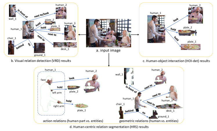
Figure 1: Comparison of the proposed HRS task with VRD and HOI-det.

Targeted at problems that require fine-grained details, we propose a new task — human-centric relation segmentation (HRS), which is a fine-grained case of human-object interaction detection (HOI-det). HRS aims to predict the relations between human and its surrounding entities and identify the relation-correlated human parts, which are represented as pixel-level masks. In this paper, we use entity to include thing and stuff.

This new HRS task is partially related to Visual Relation Detection (VRD) [11, 12, 13, 14, 15] which aims at understanding the relations between entities in the image, and HOI-det [16, 17] which tries to estimate the relations between human and surrounding objects. An illustration of VRD, HOI-det and HRS is shown in Figure 1. Given an input image in Figure 1a, VRD generates several $\langle$subject, relation, object$\rangle$ triplets, such as $\langle$human_1, next to, desk_1$\rangle$, as shown in Figure 1b, while HOI-det outputs $\langle$human, action, object$\rangle$ triplets like $\langle$human_1, hold, plate_1$\rangle$, which focuses on the relations between human and objects it interacts with, as shown in Figure 1c. Both VRD and HOI-det adopt bounding boxes to represent the subject and object regarding a certain relation. By contrast, our HRS task adopts pixel-level masks to represent both subject and object, and divides relations into two different types, as shown in Figure 1d. The first type of relation is called action relation defined between specific human parts and the corresponding entity, e.g. $\langle$human_1 [right arm], hold, plate_1$\rangle$. The subjects corresponding to such relations are human parts correlated to action rather than the whole human body. The other type is geometric relation defined between human and the corresponding entity that describes relative positions, like $\langle$human_1, behind, chair_1$\rangle$.

TABLE I: Comparison of VRD, HOI-det and HRS. Notations “part”,“geo” and “seg” denote “human part”, “geometric” and “segmentation” respectively.

Task	Subject	Relation	Object	Representation
VRD	entity	action+geo	entity	box
HOI-det	human	action	thing	box
HRS	human+part	action+geo	entity	seg

Compared with VRD and HOI-det, HRS can capture not only the relative position information, but also the detailed action information. Through the classification of interacted human parts , HRS can distinguish $\langle$human [left arm], throw, ball$\rangle$ and $\langle$human [both arms], throw, ball$\rangle$. The HRS adopts the more expressive mask representation rather than bounding boxes, which can describe exact entity shapes and contain little background area and thus is fairly beneficial to downstream tasks. Also, the masks are more suitable for representing stuff, such as sky or ocean, which has no fixed shape and is often non-convex. A summary of comparisons among VRD, HOI-det and the proposed HRS is given in Table I.

Since existing datasets either have no part level relation annotations or no mask segment annotations, we collect and annotate a large high-resolution dataset, called Person in Context (PIC), to facilitate research on the new HRS task. The PIC dataset contains $17,122$ images with both segmentation and relation labels. For segmentation, we densely label $141$ kinds of thing and stuff entities. We also label $25$ human parts and $16$ human key points. For relation, we label $14$ action relations and $9$ geometric relations.

In addition, we propose a Simultaneous Matching and Segmentation (SMS) framework to solve the new HRS task, with compact structure and simple design. SMS contains three parallel branches. 1) An entity segmentation branch segments entities in the image by identifying their centers and corresponding masks. To detect the entity centers, we estimate entity center heatmaps whose highest responses correspond to the locations and categories of the entity centers. To generate the masks, we produce mask kernels and mask features in parallel. Depending on the location of the detected entity center, a specific location-aware mask kernel is dynamically generated and convoluted with the mask feature to generate the mask of the entity. 2) A subject object matching branch pairs the human with its interacted entities and identifies their relations. Concretely, we detect the relation point (the middle point of the subject and object), and also estimate the displacements between each relation point and the subject/object as well as classify the human parts involved in the interaction. The subject and object linked by the same relation point are paired and form a triplet. 3) A human parsing branch produces semantic human parsing. The results produced by these three branches are fused to generate the final HRS result. SMS is able to achieve $36$ FPS for $512\times 512$ sized images in the $\text{Recall}@25$ setting. In addition, we extensively benchmark the dataset with the baselines modified from state-of-the-art VRD and HOI-det methods.

Our contributions can be summarized as follows. 1) We propose a new human-centric relation segmentation task, which can benefit a lot of cognitive-like tasks. HRS is a fine-grained case of HOI-det. 2) We collect, annotate and release a large high-resolution Person in Context (PIC) dataset for facilitating exploring the task. 3) we propose an one-stage Simultaneous Matching and Segmentation (SMS) framework, which integrates the entity segmentation and human-centric relation prediction in an unified model, achieving competitive performance at real time inference speed. Both the PIC dataset and the proposed SMS method will be released at http://picdataset.com/challenge/index/.

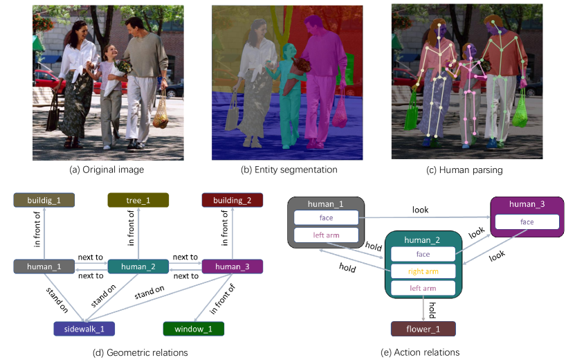
Figure 2: An example of the PIC dataset. For an image (a), both the entity segmentation (b) and human parsing (c) are labelled. We also label geometric and action relations. In the geometric relation graph (d), the nodes are entity instances of (b) while the edges are spatial relations. In the action relation graph, there are two kinds of nodes. The non-human nodes are also entity instances of (b) while the human nodes contain the interacted human parts in (c) which make the action.

2 Related Work

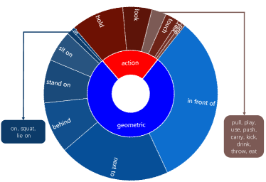
Figure 3: Distribution of action and geometric relations.

2.1 VRD and HOI-det

VRD aims to detect the relation triplets composed of subject, relationship and object in the input image. Most existing VRD methods follow a two-step pipeline including object detection and relation estimation. Existing research mostly focuses on the second step. Lu et al. proposed a two-way framework that finetunes the likelihood of a predicted relationship using language priors from semantic word embeddings [18]. Xu et al. introduced a method to pass message between objects and relations to improve triplet predictions [19, 12, 20]. Zhang et al. attempted to learn the relation in a low-dimensional space [13]. Recently, the graph convolution [21] is used to gather the information from different nodes [14].

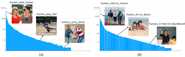
Figure 4: (a) Distribution of action triplets and (b) distribution of geometric triplets.

HOI-det as a special case of the VRD task, aims to detect the action relations with subjects specified to be “human”. HOI-det needs to estimate the bounding boxes of human and object as well as their relations, e.g., actions and geometric relations. Most previous methods follow a two-stage pipeline, first detecting all candidate subjects and objects and then predicting their interactions. Pang et al. proposed a contextual attention framework to exploit the rich context information that is crucial for HOI prediction [22]. GPNN uses a message passing mechanism to reason upon graph structured information [23]. Feng et al. proposed a turbo learning method which views human pose and HOI as complementary information to each other and optimize both tasks in an iterative manner [24]. Our proposed HRS explores the geometric relations and action relations between humans and entities. Moreover, it requires fine-grained classification on the human parts that make the actions. We propose a one-stage method that contains parallel branches, the intermediate results of which can be fused to form HRS results.

Both [25] and our method detect the relations by combining relation point detection and interaction grouping. Compared with traditional HOI-det methods, both [25] and our method directly detect relation from the whole feature map, thus utilizing richer context and reducing the computational cost that originally scales quadratically with the number of entities. The differences between [25] and our method lie in the following aspects. ($i$) The two methods are designed for different tasks.  [25] tackles HOI-det, while we tackle HRS which provides fine-grained understanding of human and the surrounding environment. ($ii$)  [25] adopts an extra and independent detector to detect the entities, while our method integrates entity segmentation into the unified SMS framework. Thus our method is more compact and fast during inference. ($iii$) Both methods contain similar keypoint-based relation point detection modules. But their object/entity detection modules are different. Specifically, [25] adopts anchor-based Faster R-CNN [26] as the object detector, which is inconsistent with the keypoint-based relation point detection module. But in our method, the entity detection is conducted in a keypoint-based manner. Thus both our entity detection module and relation point detection module are keypoint-based and thus consistent, which enables the latter to benefit from the former. ($iv$)  [25] defines the interaction point as the midpoint between the bounding box center of subject and object, while our method defines the relation point as the midpoint between the mass center of subject and object segments, which is tailored for our relation segmentation task.

2.2 Instance Segmentation and Relation Segmentation

Instance segmentation aims to detect the instances in the image and represent them by pixel-level masks. We follow the instance segmentation methods to obtain the masks for subjects and objects of detected relations. Instance segmentation methods can be roughly divided into two kinds. First, detection-based methods achieve successful segmentation relying on the object proposals [27, 27, 28]. Li et al. proposed a FCN that adopts position-sensitive score maps to detect and segment objects simultaneously [29]. Mask R-CNN [30] is built on the Faster R-CNN and uses an additional mask branch to generate object masks. Chen et al. introduced a cascade architecture to interweave detection and segmentation, and progressively refine both results [31]. Fu et al. built an instance segmentation model on single-shot detectors, retaining fast inference speed and showing competitive accuracy [32]. Second, detection-free methods where the instance masks do not rely on the pre-detected bounding boxes are also very popular. For example, some metric learning based methods [33, 34, 35] learn an embedding for each pixel and cluster the pixels that are close in the embedding space to generate instance masks. Recently, Polarmask [36] represents the instance masks by discrete contour points and directly regresses the contour points. SOLO [37] assigns instance masks to specific instance categories according to locations and scales, converting instance masks prediction to a simpler classification problem. SOLOv2 [38] learns adaptive mask kernels and mask features to generate the mask for each instance conditioned on the instance location. Our method follows the SOLOv2 mechanism to get the mask of both human and surrounding entities (thing and stuff) to achieve accuracy-speed trade-off.

[39] proposes a multi-stage network which progressively refines the instance segmentation and relation prediction according to the output of its previous stage. The differences between [39] and our method is that they build the instance localization network and an interaction recognition network work in a cascade manner. More specifically, an instance localization network first generates human and object proposals, and then an instance recognition network identifies the action for each human-object pair. Thus their method suffers from large computational cost and prediction latency. To the contrary, our method establishes a simultaneous matching and segmentation framework, where both the entities and their relations are estimated by keypoints heatmap in the one-stage model with much less complexity.

2.3 Human Parsing

In HRS setting, the subject of one action relation is set as the relation-correlated human parts. Thus HRS requires human part segments which can be obtained through human parsing. Human parsing has received increasing interest over recent years [40, 41, 42]. Liang et al. introduced a large-scale dataset LIP and proposed a self-supervised structure-sensitive learning approach [43]. Gong et al. collected a multi-human parsing dataset and proposed a detection-free model [44]. Zhao et al. presented a fine-grained multi-human parsing dataset MHPv2 and proposed a nested adversarial network model [45]. In our HRS task, we estimate the actions between human parts and surrounding entities

face	hair	coat	uppercloth	left_arm
right_arm	pants	left_leg	right_leg	skin
beard	headwear	jewelry	dress	skirt
left_shoe	right_shoe	bag	tie	hat
scarf	sunglasses	gloves	socks	belt

(a) 25 Human parsing labels.

head_top	upper_neck	thorax	left_shoulder
right_shoulder	left_elbow	right_elbow	left_wrist
right_wrist	pelvis	left_hip	right_hip
left_knee	right_knee	left_ankle	right_ankle

(b) 16 Human pose labels.

TABLE II: Human parsing and pose labels.

3 Person In Context Dataset

In this section, we introduce the collected PIC dataset for the HRS task. We have spent nearly three years to continuously refine the dataset. Notably, we organized ECCV 2018 the 1st PIC workshop/challenge and ICCV 2019 the 2nd PIC workshop/challenge, which attracted worldwide competitors. The feedbacks from the participants have also been explored to help refine the dataset. In this paper we provide the latest version (a.k.a PIC 3.0) which is different from that used in ECCV 18 and ICCV 19 challenges. In future, we will keep refining it by collecting more images with strict copyright verification and labeling more diverse relations.

3.1 Data Collection

The data collection is done with three steps.

1. Data crawling: PIC contains both indoor and outdoor images, which are crawled from Flickr website with copyrights. Query words for retrieving indoor pictures include cook, party, drink, watch tv, eat, etc., and those for outdoor ones include play ball, run, ride, outing, picnic, etc. In this way, the collected data enjoy great diversities in terms of scenario, appearance, viewpoint, light condition and occlusion.

2. Data filtering: We filter out the images with low resolution or without human. Then we calculate the distributions of the relations. We note that the relation distribution shows a long tail.

3. Data balancing: We recollect the data for relations with lower frequency to balance the data distribution. Therefore, the long tail effect is alleviated to some extent.

TABLE III: Comparison with existing datasets.

Dataset	Stuff	Segmentation	Relation	Human part	Human Pose	Average resolution
Visual Gennome[11]	✓	$\checkmark$	✓	$\times$	$\checkmark$	413*500
VRD[18]	✓	$\times$	✓	$\times$	$\times$	764*950
VCOCO [16]	$\times$	$\checkmark$	✓	$\times$	$\checkmark$	481*578
HICO-DET [17]	$\times$	$\times$	✓	$\times$	$\times$	497*593
PIC	✓	✓	✓	✓	✓	1427*1882

3.2 Data Annotation

We sequentially label the entity segmentation and relations. For “human” entities, we densely annotate the human part segments and human keypoints. Two kinds of relations (action and geometric relations) are annotated between humans and surrounding entities. The detailed annotation procedure is as follows:

Entity segmentation: We first annotate $141$ kinds of things and stuff in the images. The entity categories cover a wide range of indoor and outdoor scenes, including office, restaurant, seaside, snowfield, etc. For each entity falling into predefined categories, we label it with its class and pixel-level mask segment. The disconnected regions of stuff are viewed as different entities. Some examples are shown in Figure 2b.

Human parts & human keypoints: Human part segments and human keypoints are annotated for all the “human” entities. Our dataset also provides human keypoints annotation in order to facilitate the follow-up study. As shown in Table II(a) and Table II(b), we annotate $25$ different human parts inspired by ATR dataset [41]. As shown in Table II(b), we annotate $16$ different human keypoints following the definition of [45, 46]. Some human pose and parsing examples are shown in Figure 2c.

Relation: We annotate relations between the annotated “human” entities and their surrounding entities. We define 14 kinds of geometric relations and 9 kinds of action relations which are common in daily expressions.

Geometric relations are defined upon the human and surrounding context. Some examples are shown in Figure 2d, such as $\langle$human_2, next to, human_3$\rangle$ and $\langle$human_2, in front of, tree_1$\rangle$.

Action relations are defined between the human part and the interacted entities. Some action relations are shown in Figure 2e, like $\langle$human_2 [left arm], hold, flower_1$\rangle$ and $\langle$human_1 [left arm], hold, human_2$\rangle$, etc.

Note that there may exist multiple relations between different human parts and an object. For example, $\langle$human [face], look at, ball$\rangle$, $\langle$human [left arm], hold, ball$\rangle$ and $\langle$human [right arm], hold, ball$\rangle$ may co-exist. Moreover, there may even exist multiple relations between one human part and one object. For example, $\langle$human [left arm], hold, phone$\rangle$ and $\langle$human [left arm], use, phone$\rangle$ may co-exist. Besides, geometric relations are not exclusive either. For example, $\langle$human_1, next to, human_2$\rangle$ and $\langle$human_1, in front of, human_2$\rangle$ may co-exist.

3.3 Dataset Statistics

The PIC dataset contains $17,122$ images with $141$ categories of entity segments, $23$ kinds of relations between human and entities. Each human is annotated with $25$ different human parts and $16$ human keypoints. PIC contains $8.1$ entities (including $3.8$ human entities) and $10.4$ relations per image on average.

The distribution of entities is shown in Figure 5. The most frequent is “human”. The “ground” also occurs frequently. On the contrary, “surfboard” and “ice” rarely occur. The distribution of relations is shown in Figure 3 and 4. The geometric relations are more frequent, and both geometric and action relations have long-tailed distributions.

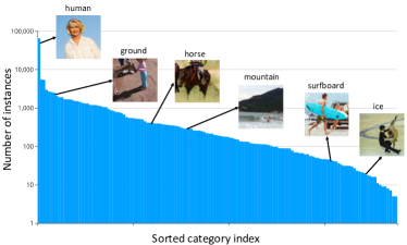
Figure 5: Distribution of things and stuff.

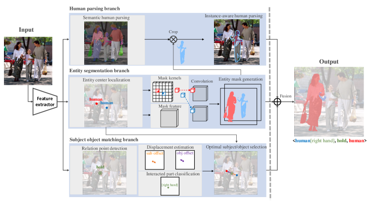
Figure 6: Framework of the proposed SMS. It is composed of a feature extractor and three parallel branches. The entity segmentation branch detects entities centers and describes them by masks. The subject object matching branch pairs the corresponding subjects and objects and identifies their relations. The human parsing branch segments the semantic human parts. All these intermediate results are fused to generate the HRS results.

PIC is split into $12,339$, $1,916$ and $2,867$ images for train, val and test set respectively. Some examples of our extensively annotated PIC dataset are shown in Figure 2.

3.4 Comparisons with Existing Datasets

As shown in Table III, we compare our PIC dataset with several other popular datasets. Similar with VRD datasets like Visual Genome [11] and VRD [18], PIC labels the relations among things and stuff. Comparatively, the HOI-det datasets like VCOCO [16] and HICO-DET [17] only label the relations between human and things. In addition, PIC has per-pixel masks to describe the entities more precisely, especially when the subjects or objects belong to stuff type. V-COCO and Visual Genome also contain mask annotations brought from the original COCO dataset, but mask annotations in PIC have higher quality and better boundary consistency. PIC also labels human poses and human parsing to facilitate the detailed inference of interacted human parts. Moreover, PIC is a high-resolution dataset with its average resolution significantly larger than other existing datasets, supporting fine-grained recognition of human and its context.

4 Our method

4.1 Overview

We propose a single-stage Simultaneous Matching and Segmentation (SMS) method to solve the HRS task. The framework is shown in Figure 6. It contains a feature extractor and three parallel branches including the entity segmentation branch, the subject object matching branch and the human parsing branch. Given an input image $I\in\mathbb{R}^{H^{0}\times W^{0}\times 3}$, the extracted feature is $F\in\mathbb{R}^{H\times W\times d}$, where $\left({H,W}\right)=\left({H^{0}/s},{W^{0}/s}\right)$ and $s$ is the output stride. If not specified, the coordinates in the remaining of this paper are relative to the $H\times W$ feature size.

The entity segmentation branch detects the entities in the image and describes them with the pixel-level masks. The subject object matching branch detects the existence of any relations and locates the corresponding subjects and objects. For geometric relations, the subject are human instances, while for action relations, the subjects are further defined as interacted human parts. The human parsing branch decomposes humans into several semantic human parts, serving for interacted parts localization regarding the action relations. Afterwards, the intermediate results are fused to produce the HRS results. Next, we will describe our framework in detail.

4.2 Entity Segmentation Branch

To output the pixel-wise masks for the entities (subjects and objects), SMS contains an entity segmentation branch with an entity center localization module and an entity mask generation module.

Entity center localization: We detect the center coordinates $\left(x,y\right)\in\mathbb{R}^{2}$ and its class label $c$ for each entity. Since directly detecting the center point is difficult, we follow the key-point estimation methods [47] to splat a point into a heatmap with a Gaussian kernel. As shown in Figure 6, given an input image $I$, the entity center heatmap ${Y}\in\mathbb{R}^{H\times W\times C_{ent}}$ is estimated, where $C_{ent}$ is the number of entity categories including “human” and other $C_{ent}-1$ entity categories. If the center of an entity belonging to the $c^{th}$ category is located at $\left(x^{0},y^{0}\right)$ in the input image $I$, then the entity center heatmap ${Y}$ will have a high response value at $\left({x,y,c}\right)$, where $\left({x,y}\right)=\left(\left\lfloor{x^{0}/s}\right\rfloor,\left\lfloor{y^{0}/s}\right\rfloor\right)$.

To balance the positive and negative points, we use focal loss [48, 49] on the center heatmap. Given the ground truth heatmap $\hat{Y}$ and the predicted heatmap $Y$, the mask center localization loss $L_{ent}$ is defined as

$${L_{ent}=-\frac{1}{N^{pos}}\sum\limits_{xyc}\begin{cases}\left(1-{Y}_{xyc}\right)^{\alpha}{\log\left({Y}_{xyc}\right)}\;&\text{if}~{}\hat{Y}_{xyc}=1,\\[8.53581pt] \begin{gathered}({1-\hat{Y}_{xyc}})^{\beta}\left(Y_{xyc}\right)^{\alpha}\\ {\log\left({1-{Y}_{xyc}}\right)}\end{gathered}&\text{otherwise}.\end{cases}}$$ (1)

In Equation (1), $N^{pos}$ is the number of ground truth entities. The hyper-parameters $\alpha$ and $\beta$ are set to $2$ and $4$.

Entity mask generation: Inspired by SOLOv2 [38], we adopt a location-aware entity mask generation method that firstly learns mask kernels and mask features in parallel, and then applies $1\times 1$ location-aware convolution kernel on the mask features to produce the mask. More concretely, the mask kernels are of the size $M_{kernel}\in\mathbb{R}^{S\times S\times D}$, where the input image is divided into $S\times S$ grids and each grid cell stands for a unique location-aware convolution kernel. If the mask center of an entity falls into one grid cell at $(i,j)$, its corresponding location-aware mask kernel ${M^{i,j}_{kernel}}\in\mathbb{R}^{1\times 1\times D}$ is selected from $M_{kernel}$. Then ${M^{i,j}_{kernel}}$ is convolved with the mask feature $M_{feat}\in\mathbb{R}^{H\times W\times D}$ to generate the entity mask $m_{i,j}\in\mathbb{R}^{H\times W}$.

The loss function of entity mask generation is

$$L_{mask}=\frac{1}{N^{pos}}{\sum\limits_{(i,j)\in S^{pos}}{d_{mask}\left(m_{i,j},\hat{m}_{i,j}\right)}},$$ (2)

where $N^{pos}$ is the number of ground truth entities and $S^{pos}$ is the set of center coordinates of ground truth entities. $m_{i,j}$ and $\hat{m}_{i,j}$ are the predicted mask and ground truth mask. $d_{mask}\left(\cdot\right)$ can be any type of segmentation loss function. Here Dice Loss is chosen.

4.3 Subject Object Matching Branch

Suppose $M$ entities are segmented. There exist $M(M-1)$ kinds of possible combinations. Traditional VRD methods traverse all combinations, which is quite time consuming.

In order to pair the related subject and object, we introduce a relation point $\left({x_{r},y_{r}}\right)=\left(\left\lfloor\frac{x_{s}+x_{o}}{2}\right\rfloor,\left\lfloor\frac{y_{s}+y_{o}}{2}\right\rfloor\right)$, which is the midpoint of the corresponding subject center $\left({x_{s},y_{s}}\right)$ and object center $\left({x_{o},y_{o}}\right)$. Moreover, we estimate the displacement between the relation point $\left({x_{r},y_{r}}\right)$ and subject center $\left({x_{s},y_{s}}\right)$, denoted as $\left({d_{r}^{sx},d_{r}^{sy}}\right)$. Thus the matched subject is supposed to be around $\left({x_{r}+d_{r}^{sx},y_{r}+d_{r}^{sy}}\right)$. Similarity, we can estimate the displacement between the relation point and object center, denoted as $\left({d_{r}^{ox},d_{r}^{oy}}\right)$. Thus the matched object is supposed to be around $\left({x_{r}+d_{r}^{ox},y_{r}+d_{r}^{oy}}\right)$. Thus the relation point serves as the route to match the corresponding subject $\left({x_{r}+d_{r}^{sx},y_{r}+d_{r}^{sy}}\right)$ and object $\left({x_{r}+d_{r}^{ox},y_{r}+d_{r}^{oy}}\right)$. Next, we will elaborate how to detect the relation point and estimate the two displacements.

Relation point detection: we define the relation point as the middle of subject and object centers. Thanks to the large respective field of the network, the relation point is able to capture sufficient relation detection information. The relation point is detected in a similar way with the above mentioned entity center localization. As shown in Figure 6, a relation point heatmap $P\in\mathbb{R}^{H\times W\times C_{rel}}$ is generated, where $C_{rel}$ is the number of relation categories including action relations like “hold” and geometric relations like “in front of”. The responses around $\left(x_{r},y_{r},c\right)$ in $P$ will be high, where $c$ is the corresponding relation category.

Displacements estimation: In addition, for each relation $r$, we estimate the displacement from the relation point to the corresponding subject/object center, which is denoted as $\left({d_{r}^{sx},d_{r}^{sy}}\right)$ and $\left({d_{r}^{ox},d_{r}^{oy}}\right)$ respectively. Specifically, the model outputs two displacement offset maps $D_{s}$ and $D_{o}\in\mathbb{R}^{H\times W\times 2}$.

The relation point detection loss $L_{rel}$ is similar with $L_{ent}$ while the subject/object displacement estimation loss $L_{disp}$ is defined as

$$L_{disp}=\frac{1}{N^{r}}\!\sum\limits_{r\in S^{rel}}( |{d_{r}^{sx}-{\hat{d}}_{r}^{sx}}|+|{d_{r}^{sy}-{\hat{d}}_{r}^{sy}}|$$ (3)

$$+|{d_{r}^{ox}-{\hat{d}}_{r}^{ox}}|+|{d_{r}^{oy}-{\hat{d}}_{r}^{oy}}|),$$

where $N^{r}$ is the number of ground truth relations and $S^{rel}$ is the set of ground truth relations.

Interacted part classification: When the relation is an action relation, the subject of the triplet is further refined as the human parts making the action. For example, $\langle$human, hold, cup$\rangle$ can be further refined as $\langle$human [left arm], hold, cup$\rangle$ and $\langle$human, stand on, grass$\rangle$ can be further refined to $\langle$human [right shoe], stand on, grass$\rangle$. To this end, we output the probability of each human part participating in the action. It is treated as a multi-label classification task. For every relation point $\left({x_{r},y_{r}}\right)$, the branch produces a multi-hot classification result $s_{r}\in\mathbb{R}^{C_{part}}$, where $C_{part}$ is the number of human part categories.

The loss function of interacted part classification is defined as

$$L_{part}=\frac{1}{N^{r}}{\sum\limits_{r\in S^{rel}}{BCEloss\left(s_{r},\hat{s}_{r}\right)}},$$ (4)

where $N^{r}$ is the number of relation categories and $\hat{s}_{r}$ is the groundtruth part classification label. Note that we use BCEloss loss here because multiple parts may relate to the same object. For instance, both left arm and right arm may hold the cup.

4.4 Human Parsing Branch

To generate the segmentation mask for each human part, e.g. left leg, right arm, we generate human parsing results $P_{sem}\in\mathbb{R}^{H\times W\times C_{part}}$, where $C_{part}$ is the number of human part categories. The human parsing loss function $L_{human}$ is defined as

$$L_{human}=L_{ce}+L_{iou},$$ (5)

where $L_{ce}$ is the cross entropy loss widely used in semantic segmentation and $L_{iou}$ is the Lovasz loss [50] directly optimizing the intersection over union. Then, the subject segmentation result is used to crop on the human parsing result $P_{sem}$ to get the instance-specific human part segments.

4.5 Loss and Inference

The total loss of our SMS method is the weighted sum of the above mentioned losses:

$$L\!=\!L_{ent}+L_{rel}+\lambda_{1}L_{mask}+\lambda_{2}L_{disp}+\lambda_{3}L_{part}+\lambda_{4}L_{human},$$ (6)

where $\lambda_{1}$, $\lambda_{2}$, $\lambda_{3}$ and $\lambda_{4}$ are weights to balance the loss.

During inference, firstly we pick top$K_{s}$, top$K_{o}$ and top$K_{r}$ local maximum activation for subject center, object center and relation point respectively, where $K_{s}$, $K_{o}$ and $K_{r}$ are hyperparameters and set empirically. Each detected relation point finds its subject and object through an optimal subject/object selection process by Equation (7). During the process, the estimated subject center of a relation $r$ is obtained by summing the entity center localization results and displacements estimation results $\left(x_{r}\!+\!d_{r}^{sx},y_{r}\!+\!d_{r}^{sy}\right)$. Then the optimal subject $\left({x_{r}^{s},y_{r}^{s}}\right)$ is selected from all the detected subjects $S^{sub}$ according to the distances from their centers to the estimated subject center.

$$\left({x_{r}^{s},y_{r}^{s}}\right)=\!\underset{(x,y,c)\in S^{\mathit{sub}}}{argmin}\frac{1}{Y_{x,y,c}}\!\left|\left(x,y\right)\!-\!\left(x_{r}\!+\!d_{r}^{sx},y_{r}\!+\!d_{r}^{sy}\right)\right|,$$ (7)

where $S^{sub}$ is the set of detected subject center points and ${Y_{x,y,c}}$ is the value at $(x,y,z)$ in the entity center heatmap $Y$. The optimal object $\left({x_{r}^{o},y_{r}^{o}}\right)$ is selected in the same way. After localizing the subject and object, their mask kernels are selected according to the grid $(i,j)\in{S\times S}$ which $\left({x_{r}^{s},y_{r}^{s}}\right)$ and $\left({x_{r}^{o},y_{r}^{o}}\right)$ fall in. Then the subject mask $m_{sub}$ and object mask $m_{obj}$ are produced by applying the dynamically selected mask kernels on the mask feature.

For action relation triplets, the results are in the form of $\langle$human [part], action, entity$\rangle$. Specifically, we get human part classification results $s_{r}$ to identify the interacted part. Then, the interacted human part segments are generated by fusing the subject masks $m_{sub}$, semantic human parsing result $P_{sem}$ and part classification results $s_{r}$.

5 Experiments

We first compare the proposed SMS with baselines in HRS task over the PIC dataset. To further show its generalization ability, we also evaluate SMS in the Relation Segmentation (RS) task on both PIC and V-COCO datasets [16].

	Relation	RS(%)				HRS(%)
Method	Backbone	mR@$25$	mR@$50$	mR@$100$	AR	mR@$25$	mR@$50$	mR@$100$	AR	Running Time
$m$-MOTIFS[12]	VGG-16	19.89	27.90	32.78	26.86	12.62	18.01	21.43	17.36	107 ms+163ms
$m$-MOTIFS*	ResNet-50	21.36	28.57	33.54	27.82	13.90	19.10	22.67	18.56	109 ms+163ms
$m$-KERN[51]	VGG-16	21.27	29.30	34.55	28.37	13.98	19.41	22.97	18.79	149 ms+163ms
$m$-KERN*	ResNet-50	22.32	29.65	34.76	28.91	14.14	19.37	23.31	18.97	159 ms+163ms
$m$-PMFNet[52]	ResNet-50	23.01	27.85	29.50	26.79	14.90	17.74	18.87	17.17	63 ms+163ms
SMS	ResNet-50	24.42	30.52	34.96	29.97	15.81	19.42	22.45	19.23	28 ms
SMS	DLA-34	25.25	30.01	34.97	30.08	16.35	19.45	23.38	19.73	31 ms
SMS-L	ResNet-50	26.58	32.8	37.21	32.21	17.63	21.53	24.90	21.35	81 ms

TABLE IV: Comparisons on PIC test set.

Method	$AP_{role}$(%)
$m$-MOTIFS[12]	40.74
$m$-KERN[51]	41.31
$m$-PMFNet[52]	43.13
SMS	44.13

TABLE V: Comparison on VCOCO test set.

5.1 Implementation Details

We use DLA-34 network [53] and ResNet-50 [54] as our backbones to show the generalization of the proposed SMS framework. We modify the light-weight DLA network to contain a progressive refinement architecture following CenterNet [49]. We use ResNet with FPN architecture [55] to enable multi-scale predictions. The FPN layers are fused to generate single scale features according to [56]. The parameters of the backbone are initialized from the pretrained weights on ImageNet dataset [57]. All the parallel branches except the mask generation branch share the same architecture, which is composed of two (three in the relation point detection branch) $3\times 3$ convolutional layers followed by RELU and one $1\times 1$ convolutional head for prediction. In the entity segmentation branch, the heads of mask kernels and mask feature are both composed of two $3\times 3$ and one $1\times 1$ convolutional layer followed by group normalization and RELU, where the first convolution layer is CoordConv [38]. If not specified, these branches are initialized randomly and trained from scratch.

By widening and deepening three parallel branches of SMS, we obtain a larger model denoted as SMS-L. SMS-L shares the same feature extraction backbone as SMS. The difference is that SMS-L contains more parameters and thus introduces more computational cost to each parallel branch. More spcifically, for SMS-L, we stack 5 more convolutional layers followed by group normalization and ReLU before entity segmentation branch, subject object matching branch and human parsing branch respectively, with progressive summation operation for feature fusion. The numbers of convolutional layers in entity segmentation branch, subject object matching branch and human parsing branch are set to 3, 3 and 5 respectively. We also expand the feature channel in the three parallel heads from 128 to 384.

For the PIC dataset, we train for $140$ epochs with Adam [58]. The initial learning rate is 3e-4, and batch size is $60$. For the V-COCO dataset, we also train for $140$ epochs. The initial learning rate is 4e-4, and batch size is $40$. For both datasets, the learning rate is divided by $10$ at $90^{th}$ and $110^{th}$ epoch respectively. The loss weights $\lambda_{1}$, $\lambda_{2}$, $\lambda_{3}$ and $\lambda_{4}$ are set to $3$, $1$, $20$ and $5$ respectively in experiments.

The speed of our SMS model is evaluated on a single RTX $2080$Ti GPU, with Pytorch $1.1$ and CUDA $10.2$. When evaluating the inference speed, we only calculate the running time of the models and ignore the time consumption of the result saving process.

5.2 Baselines

We design several baselines for both RS and HRS tasks.

For the RS task, we modify the state-of-the-art VRD methods MOTIFS[12], KERN[51] and HOI-det method PMFNet[52] to produce the entity segmentation results. These methods rely on a strong object detector Faster R-CNN [59] to generate object candidates and then infer their relations, which follow a two-stage pipeline. These modified RS baselines are denoted as $m$-VRD, $m$-MOTIFS and $m$-PMFNet respectively. More specifically, we replace the Faster R-CNN in these methods with Mask R-CNN [30] with ResNet-50 backbone to generate entity masks. The $m$-PMFNet does not use human pose features for fair comparison.

For the HRS task, to produce human part level segmentation, a human parsing head is attached to the Mask R-CNN to output instance-level human parsing results. To identify which is the interacted part, several additional fully connected layers are added in parallel with the original relation prediction head. The human parsing results, interacted part classification results, together with the relation prediction results are merged to form the final HRS results.

5.3 Evaluation Metric

The widely used average precision metric is not suitable for PIC on account of some potential relations not annotated which may cause a lot of misclassified “false positive” samples. We use mean $\text{Recall}@K$ (abbr. mR) rather than $\text{Recall}@K$ to evaluate both RS and HRS following [15], considering the reporting bias as discussed in [60].

For RS and HRS, a predicted relation triplet is regarded as a True Positive (TP) sample if it matches with any ground truth relation triplet in following respects: 1) the subject, object and relation categories are both consistent with the ground truths, and 2) the IoU between predicted truth subject mask and ground subject mask is above a threshold $\tau_{iou}$, and the same case for the object.

Mean Recall@$K$ is the mean of Recall@$K$ per relation category. The most $K$ confident relation triplets are used for evaluation. We calculate mR@$K$ as

$$\normalsize\text{mR}@K\!=\!\frac{1}{\left|S^{\tau}\right|}\sum\limits_{\tau_{iou}\!\in S^{\tau}}\frac{1}{C}\sum\limits_{c\in[1...C]}\Big{(}{\sum\limits_{p\in P_{c}}\mathbbm{1}_{\{p~{}\text{is TP}\}}}\Big{)}/\left|G_{c}\right|,$$ (8)

where $\left|\cdot\right|$ is the cardinality of a set, $S^{\tau}\!=\!\{0.25,0.5,0.75\}$ and $\tau_{iou}$ is the IoU threshold for assigning predicted subjects and objects to ground truth, $C$ is the number of relation categories, $P_{c}$ is the set of predicted triplets belonging to relation type $c$ and $\sum\limits_{c}\left|P_{c}\right|\leq K$, $G_{c}$ is the set of ground truth triplets belonging to the relation type $c$.

The corresponding response values in the heatmap are the confidences of detected entities and relationships. Confidence of a relation triplet is calculated by multiplying the confidences of subject, object and relationship. To comprehensively evaluate the method, we also adopt AR which is the mean of mR@$25$, mR@$50$ and mR@$100$.

5.4 Experiments on PIC Dataset

We evaluate performance on both RS and HRS tasks. Different from VRD, RS uses pixel-level masks to represent entities rather than bounding boxes. The quantitative results are shown in Table IV. In their original papers, MOTIFS [12] and KERN [51] use VGG-16 as the feature extractor backbone. For fair comparison, we re-implement these two baselines using more powerful ResNet-50, which are denoted as $m$-MOTIFS* and $m$-KERN*. For the RS task, SMS-L achieves the best performance of $32.21$% AR in RS, which is $3.3$% higher than $m$-KERN* and $4.39$% higher than $m$-MOTIFS*. Moreover, the improvements over baselines are consistent in all evaluation metrics from $\text{mR}@25$ to $\text{mR}@100$. For the HRS task, SMS-L also achieves the best accuracy of $21.35$% AR, which is $2.38$% higher than $m$-KERN* and $2.79$% higher than $m$-MOTIFS*. It indicates that SMS-L is able to recognize humans, objects and their relations at a finer level. Moreover, SMS-L outperforms SMS at the cost of inference latency.

We have implemented SMS with DLA-34 and ResNet-50 to show its generalization ability. For $m$-MOTIFS* and $m$-KERN*, the results with ResNet-50 are better than VGG-16. For SMS, ResNet-50 can produce faster inference but slightly lower performance than DLA-34. With both backbones, SMS achieve higher AR than all baselines in both RS and HRS settings. It shows that SMS is a general framework and not limited to a specific backbone.

Moreover, we evaluate the inference speed using the $\text{mR}@25$ setting in HRS. Specifically, the hyper parameters $K_{s}$, $K_{o}$ and $K_{r}$ are set to $25$, $10$ and $30$ respectively. The running time does not include the time consumption of data reading and result saving. Note that the running time of baselines include two parts. For example, the running time of $m$-PMFNet is composed of relation prediction time (63ms) and instance segmentation time (163ms). SMS reaches $32$ FPS (with DLA-34) and $36$ FPS (with ResNet-50) and is the only method achieving real-time inference speed. ResNet-50 is slightly faster than DLA-34, but the AR is slightly lower. The results show that the single-stage architecture of SMS achieves better speed-accuracy trade off than the two-stage baselines.

Table VI shows the results of geometric and action relations. The performance of SMS-L exceeds the baselines significantly in terms of both geometric and action relations. Especially for action relations, our method performs much better than the baselines. The reason lies in that we predict relations directly from the whole feature map, reducing the error introduced by imperfect detection results and retaining more context beneficial for action relation prediction. In sum, our method performs the best for both geometric and action relations, in both RS and HRS tasks with much less inference time.

.

TABLE VI: Performance on geometric (Geo) and action (Act) relations with ResNet-50 backbone.

	RS			HRS
Method	Geo	Act	Mean	Geo	Act	Mean
$m$-MOTIFS*[12]	32.84	24.35	28.60	32.64	8.67	20.75
$m$-KERN*[51]	32.68	26.17	29.43	32.68	8.78	20.73
$m$-PMFNet[52]	26.89	26.72	26.81	26.89	10.43	18.66
SMS-L	33.68	31.19	32.44	33.68	12.82	23.25

We define the categories of relationships which appear less than $800$ times in our dataset as the rare relations. Table VII shows the comparison on rare and non-rare relations. It can be seen that our larger model SMS-L achieves best performance on both rare relations and non-rare relations.

TABLE VII: Performance on rare and non-rare relations with ResNet-50 backbone.

	RS			HRS
Method	Rare	Non-Rare	Mean	Rare	Non-Rare	Mean
$m$-MOTIFS*[12]	17.30	35.11	26.20	7.56	26.17	16.87
$m$-KERN*[51]	19.44	35.12	27.28	7.43	25.86	16.65
$m$-PMFNet[52]	21.05	31.07	26.06	11.62	21.00	16.31
SMS-L	22.61	38.86	30.73	13.96	26.47	20.22

5.5 Experiments on V-COCO Dataset

The large-scale HOI-det dataset V-COCO [16] is annotated on a subset of COCO. V-COCO treats the objects associated with actions as different semantic roles including a direct object or an instrument object. For V-COCO, evaluation is conducted on these two types of roles separately. We extend V-COCO annotations with the original COCO annotations to generate RS annotations by simply replacing the bounding box annotations with mask annotations. Because V-COCO does not contain human parsing and interacted parts annotations, we do not evaluate the performance of HRS in this experiment. We modify the standard evaluation metric $AP_{role}$ proposed for V-COCO benchmark to evaluate the RS results. An estimated RS result is treated as true positive if both the predicted subject mask and object mask have IoU over $0.5$ with any ground truth subject mask and the corresponding ground truth object mask given the action category.

We evaluate SMS on the customized V-COCO dataset with the baselines. Table V reports the performances on the test set. Slightly different from Table IV, the performance of HOI-det method $m$-PMFNet is better than the VRD method $m$-KERN here. The observation accords with the intuition since KERN is designed for VRD and PMFNet for HOI-det. Table V shows SMS is able to achieve $44.13\%$ $AP_{role}$ with a performance gain of $1.00$% $AP_{role}$ over $m$-PMFNet and $2.82\%$ over $m$-KERN. The improvements show the effectiveness and generalization ability of SMS.

5.6 Ablation Studies

Here we evaluate different components of SMS on PIC test set. According to Table IV, DLA-34 achieves higher performance than ResNet-50. Thus we use DLA-34 backbone for the ablation studies. If not specified, all the results are evaluated in terms of the AR metric.

5.6.1 Feature Extractor

We use ResNet [54] and DLA network [53] as the feature extraction backbones. Both backbones can generate multi-level features of different scales. We further explore how SMS works with the largest single level feature map or multi-level feature fusion. To fuse multi-level features, we put the multi-level features through a series of convolution layers and upsample layers, and then fuse them with summation (for ResNet) or concatenation (for DLA network) [56].

As shown in Table IV, SMS with ResNet achieves higher inference speed while SMS with DLA achieves higher accuracy. The DLA is slightly slower than ResNet. This is because to enlarge the receptive field for the light-weight DLA network, we induce Deformale ConvNets [61] in the DLA architecture following [49]. Moreover, SMS with both backbones outperforms baselines with real-time inference speed, revealing the generalization of the proposed framework. From Table VIII, we can see multi-level features fusion also brings some performance gains for both backbones in both tasks.

Feature Extractors		RS(%)	HRS(%)
DLA-34 single-level		29.87	19.73
+multi-level feature fusion		30.08	19.73
ResNet-50 single-level		29.00	19.08
+ multi-level feature fusion		29.97	19.23

TABLE VIII: Comparisons of different feature extractors.

5.6.2 Entity Segmentation Branch

To validate the generalization ability of SMS, we replace the entity segmentation branch with two one-stage instance segmentation methods including PolarMask [62] and SOLO [37]. PolarMask [62] tackles the mask generation problem as the contour estimation problem and regresses contour polygons from the instance center. SOLO [37] learns the spatial-sensitive instance features and predicts the pixel-level masks for each instance conditioned on their locations. SMS adopts the SOLOv2 [38] to segment the entity. We only use the largest single-level feature map as the feature extractor.

Table IX demonstrates that SMS can generalize to different mask generation methods. In detail, SMS with PolarMask underperforms the other two models. It is mainly because PolarMask approximately represents the mask of the entity by polygons which have a fixed number of vertices (typically $36$). The approximate representations have a limited expressive ability especially when describing stuff classes. Actually, it is in agreement with our claim that box-like representation is not able to accurately describe the entity shape, which is exactly the motivation of our introducing the relation segmentation task. Moreover, the experiment results indicate the SMS framework is very flexible and its performance can be further boosted along with the latest developments of segmentation methods.

Segmentation Method		RS(%)	HRS(%)
PolarMask [62]		19.88	13.75
SOLO [37]		27.66	18.11
SMS		29.87	19.73

TABLE IX: Comparisons of different mask generation methods.

5.6.3 Subject Object Matching Branch

We study the effectiveness of displacement estimation and interacted part classification in SMS.

Displacement estimation: As introduced in Section 4.3, we estimate a subject offset $\left({d_{r}^{sx},d_{r}^{sy}}\right)$ and an object offset $\left({d_{r}^{ox},d_{r}^{oy}}\right)$ for the relation point $\left({x_{r},y_{r}}\right)$. Another strategy is to estimate the object offset with the negative of subject offset $\left({d_{r}^{ox},d_{r}^{oy}}\right)=-\left({d_{r}^{sx},d_{r}^{sy}}\right)$. As shown in Table X, if estimating the subject offset only, the performance is nearly the same as estimating both subject and object offsets ($29.87\%$ vs $29.71\%$ in RS task and $19.74\%$ vs $19.65\%$ in HRS task). It shows that SMS is able to accurately estimate the relation point which is the midpoint of the related subject and object pair. Therefore there is no obvious differences between estimating two offsets and estimating subject offset only.

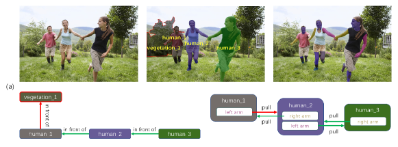
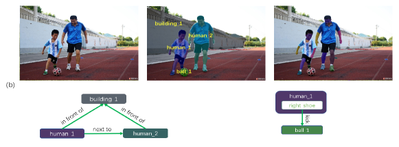
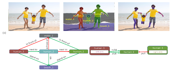
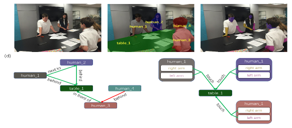
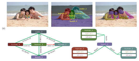
Figure 7: Visualization of HRS results on PIC test set. For each image, only $25$ most confident relation triplets are shown. In each result set, the upper row shows the original image, entity segmentation masks and interacted human part segments. The lower row are the geometric and action relation graph. In both graphs, green and red arrows stand for true positives and false negatives. Nodes with red border are ground truth masks not matched by the entities in the top 25 relations.

Displacement Estimation Method		RS(%)	HRS(%)
subject offset + object offset		29.87	19.73
subject offset only		29.71	19.65

TABLE X: Comparisons of different displacement estimation strategies.

Interacted part classification: SMS also estimates the interacted part for each relation point. We compare with three other straightforward statistic-based baselines including “Sample by distribution”, “Most frequent” and “Nearest Part”. In detail, we first calculate the frequencies/distribution of each interacted part category given the action relations. For example, “left arm” co-exists more frequently with the action “hold” than “left shoe”. “Sample by distribution” means sampling the interacted part category according to their distribution conditioned on the estimated action. “Most frequent” means directly selecting the most frequent interacted part category conditioned on the estimated action. “Nearest Part” determines the interaction body part according to their distance to the interaction point.

We evaluate the three interacted parts classification methods and the results are shown in Table XI. AR is evaluated only for action relations and geometric relations are ignored. The results show that “Sample by distribution” and “Most frequent” are able to correctly predict the interacted human parts to some extent because of the data bias. However, our SMS outperforms “Sample by distribution”, “Most frequent” and “Nearest Part” by $2.64$%, $1.56$% and $3.14$% respectively. It shows that the BCEloss in Equation 4 applied on the relation point can guide our model to distinguish interacted parts. The average recall of “Nearest Part” is $9.08\%$. This inferior performance may result from the diversity of the action appearance and the error of human parsing prediction.

Classification Method	HRS(%)
Sample by distribution	9.58
Most frequent	10.66
Nearest part	9.08
SMS	12.22

TABLE XI: Comparison of different interacted part classification methods in HRS task. Evaluation is conducted on action relations only.

5.7 Qualitative Analysis

Five HRS results on PIC dataset are shown in Figure 7. We choose the top $25$ highest score relations for each example image. Each result set contains five elements, including the original image, entity segmentation masks, interacted human part segments, the geometric and action relation graph. The green and red arrows in both relation graphs stand for true positives and false negatives relations respectively. The nodes with non-red border represent entities among the predicted top 25 triplets which have IoU over 0.5 with ground truth masks, while the nodes with red border represent ground truth not matched with any entities in the top 25 predicted triplets.

In Figure 7a, SMS can correctly estimate fine-grained human-centric relations, such as $\langle$human_2 [right arm], pull, human_1$\rangle$ and $\langle$human_2 [left arm], pull, human_3$\rangle$. Notably, SMS can correctly estimate the relative depth with respect to the camera, such as $\langle$human 3, in front of, human 2$\rangle$ and $\langle$human 2, in front of, human 1$\rangle$. The ground truth relation $\langle$human_1 [left arm], pull, human_2$\rangle$ is with low confidence and thus excluded from the top 25 relations. In Figure 7b, SMS can predict the geometric relations that human_1 and human_2 are next to each other and in front of building_1. Moreover, $\langle$human_1 [right shoe], kick, ball$\rangle$ is accurately predicted. Additionally, the human arms, legs and shoes are well segmented. In Figure 7c, the geometric graph contains the true positives including $\langle$human_1, next to, human_2$\rangle$, $\langle$human_1, stand on, beach_1$\rangle$. Note that our method can estimate two action relations between a human part and another entity, such as $\langle$human_1 [left arm], hold, human_2$\rangle$ and $\langle$human_1 [left arm], pull, human_2$\rangle$. In Figure 7d, due to occlusion by human_3, human_4 is not detected. We can handle cases where two human parts of a person interact with another entity. For example, we correctly predict $\langle$human_1 [right arm], touch, table_1$\rangle$ and $\langle$human_1 [left arm], touch, table_1$\rangle$ simultaneously. Another example is, we also successfully estimate both hands of human_2 touching table_1. In Figure 7e, the stuff categories such as “water” and “beach” are accurately segmented. By referring to the geometric graph including $\langle$human_2, in front of, water_1$\rangle$, $\langle$human_2, lie on, beach_1$\rangle$ and $\langle$human_1, next to, human_2$\rangle$, we can infer the relative position of human_2 in the image. The estimated action graph is very accurate, including $\langle$human_1 [right arm], touch, beach_1$\rangle$ and $\langle$human_1 [left arm], touch, beach_1$\rangle$ etc. In sum, the results show that SMS can well infer relations between human and surrounding entities, including things and stuff. Moreover, The interacted human parts can be accurately located. In addition, our method can describe entities by accurate segmentation masks.

6 Conclusion

In this work, we introduce the new HRS task, as a fine-grained case of HOI-det. HRS focuses on the relations between humans and surrounding entities including things and stuff, and utilizes the masks to represent subjects and objects. We also propose a new PIC dataset, which is a large scale HRS dataset with rich annotations including entity segmentation, relation and human parsing. Moreover, PIC is a high-resolution dataset which contains images several times larger than popular VRD and HOI-det datasets. We organized ECCV 2018 the 1st PIC challenge and ICCV 2019 the 2nd PIC challenge using the initial versions of the PIC dataset. The challenges attracted many participating teams around the world. By integrating the feedbacks from these teams, we refined the PIC dataset to contribute the latest version in this paper. We also propose the SMS method to solve the HRS problem. SMS is able to generate segmentation results and relation detection results simultaneously and output the HRS results in one pass. Experiments on PIC and V-COCO datasets show that SMS is more efficient and effective than multiple two stage baselines. Dataset and code will be released. In further we will explore whether the HRS results can assist other high-level cognitive-like tasks, such as visual question answering and embodied AI. Moreover, we also plan to explore the video HRS problem which outputs the human entities relations and their spatial-temporal segmentation masks.

References

- [1] Abhishek Kadian*, Joanne Truong*, A. Gokaslan, A. Clegg, E. Wijmans, S. Lee, M. Savva, S. Chernova, and D. Batra, “Are We Making Real Progress in Simulated Environments? Measuring the Sim2Real Gap in Embodied Visual Navigation,” in arXiv:1912.06321, 2019.
- [2] A. Das, S. Datta, G. Gkioxari, S. Lee, D. Parikh, and D. Batra, “Embodied question answering,” in Proceedings of the IEEE Conference on Computer Vision and Pattern Recognition Workshops, 2018, pp. 2054–2063.
- [3] P. Anderson, Q. Wu, D. Teney, J. Bruce, M. Johnson, N. Sünderhauf, I. Reid, S. Gould, and A. van den Hengel, “Vision-and-language navigation: Interpreting visually-grounded navigation instructions in real environments,” in Proceedings of the IEEE Conference on Computer Vision and Pattern Recognition, 2018, pp. 3674–3683.
- [4] Y. Qi, Q. Wu, P. Anderson, X. Wang, W. Y. Wang, C. Shen, and A. v. d. Hengel, “Reverie: Remote embodied visual referring expression in real indoor environments,” in Proceedings of the IEEE/CVF Conference on Computer Vision and Pattern Recognition, 2020, pp. 9982–9991.
- [5] J. Lu, D. Batra, D. Parikh, and S. Lee, “Vilbert: Pretraining task-agnostic visiolinguistic representations for vision-and-language tasks,” in Advances in Neural Information Processing Systems, 2019, pp. 13–23.
- [6] Y.-C. Chen, L. Li, L. Yu, A. E. Kholy, F. Ahmed, Z. Gan, Y. Cheng, and J. Liu, “Uniter: Learning universal image-text representations,” arXiv preprint arXiv:1909.11740, 2019.
- [7] W. Su, X. Zhu, Y. Cao, B. Li, L. Lu, F. Wei, and J. Dai, “Vl-bert: Pre-training of generic visual-linguistic representations,” arXiv preprint arXiv:1908.08530, 2019.
- [8] S. Antol, A. Agrawal, J. Lu, M. Mitchell, D. Batra, C. Lawrence Zitnick, and D. Parikh, “Vqa: Visual question answering,” in Proceedings of the IEEE international conference on computer vision, 2015, pp. 2425–2433.
- [9] P. Anderson, X. He, C. Buehler, D. Teney, M. Johnson, S. Gould, and L. Zhang, “Bottom-up and top-down attention for image captioning and visual question answering,” in Proceedings of the IEEE conference on computer vision and pattern recognition, 2018, pp. 6077–6086.
- [10] B. Li, X. Qi, T. Lukasiewicz, and P. H. Torr, “Manigan: Text-guided image manipulation,” arXiv preprint arXiv:1912.06203, 2019.
- [11] R. Krishna, Y. Zhu, O. Groth, J. Johnson, K. Hata, J. Kravitz, S. Chen, Y. Kalantidis, L.-J. Li, D. A. Shamma et al., “Visual genome: Connecting language and vision using crowdsourced dense image annotations,” International Journal of Computer Vision, vol. 123, no. 1, pp. 32–73, 2017.
- [12] R. Zellers, M. Yatskar, S. Thomson, and Y. Choi, “Neural motifs: Scene graph parsing with global context,” in Proceedings of the IEEE Conference on Computer Vision and Pattern Recognition, 2018, pp. 5831–5840.
- [13] H. Zhang, Z. Kyaw, S.-F. Chang, and T.-S. Chua, “Visual translation embedding network for visual relation detection,” in Proceedings of the IEEE conference on computer vision and pattern recognition, 2017, pp. 5532–5540.
- [14] J. Yang, J. Lu, S. Lee, D. Batra, and D. Parikh, “Graph r-cnn for scene graph generation,” in Proceedings of the European conference on computer vision, 2018, pp. 670–685.
- [15] K. Tang, Y. Niu, J. Huang, J. Shi, and H. Zhang, “Unbiased scene graph generation from biased training,” arXiv preprint arXiv:2002.11949, 2020.
- [16] S. Gupta and J. Malik, “Visual semantic role labeling,” arXiv preprint arXiv:1505.04474, 2015.
- [17] Y.-W. Chao, Y. Liu, X. Liu, H. Zeng, and J. Deng, “Learning to detect human-object interactions,” in 2018 ieee winter conference on applications of computer vision. IEEE, 2018, pp. 381–389.
- [18] C. Lu, R. Krishna, M. Bernstein, and L. Fei-Fei, “Visual relationship detection with language priors,” in European Conference on Computer Vision. Springer, 2016, pp. 852–869.
- [19] D. Xu, Y. Zhu, C. B. Choy, and L. Fei-Fei, “Scene graph generation by iterative message passing,” in Proceedings of the IEEE Conference on Computer Vision and Pattern Recognition, vol. 2, 2017.
- [20] Y. Li, W. Ouyang, X. Wang, and X. Tang, “Vip-cnn: Visual phrase guided convolutional neural network,” in Proceedings of the IEEE Conference on Computer Vision and Pattern Recognition, 2017, pp. 1347–1356.
- [21] T. N. Kipf and M. Welling, “Semi-supervised classification with graph convolutional networks,” arXiv preprint arXiv:1609.02907, 2016.
- [22] T. Wang, R. M. Anwer, M. H. Khan, F. S. Khan, Y. Pang, L. Shao, and J. Laaksonen, “Deep contextual attention for human-object interaction detection,” in Proceedings of the IEEE International Conference on Computer Vision, 2019, pp. 5694–5702.
- [23] S. Qi, W. Wang, B. Jia, J. Shen, and S.-C. Zhu, “Learning human-object interactions by graph parsing neural networks,” in Proceedings of the European Conference on Computer Vision, 2018, pp. 401–417.
- [24] W. Feng, W. Liu, T. Li, J. Peng, C. Qian, and X. Hu, “Turbo learning framework for human-object interactions recognition and human pose estimation,” in Proceedings of the AAAI Conference on Artificial Intelligence, vol. 33, 2019, pp. 898–905.
- [25] T. Wang, T. Yang, M. Danelljan, F. S. Khan, X. Zhang, and J. Sun, “Learning human-object interaction detection using interaction points,” in Proceedings of the IEEE/CVF Conference on Computer Vision and Pattern Recognition, 2020, pp. 4116–4125.
- [26] S. Ren, K. He, R. Girshick, and J. Sun, “Faster r-cnn: Towards real-time object detection with region proposal networks,” IEEE transactions on pattern analysis and machine intelligence, vol. 39, no. 6, pp. 1137–1149, 2016.
- [27] J. Dai, K. He, and J. Sun, “Instance-aware semantic segmentation via multi-task network cascades,” in Proceedings of the IEEE Conference on Computer Vision and Pattern Recognition, 2016, pp. 3150–3158.
- [28] S. Liu, L. Qi, H. Qin, J. Shi, and J. Jia, “Path aggregation network for instance segmentation,” in Proceedings of the IEEE Conference on Computer Vision and Pattern Recognition, 2018, pp. 8759–8768.
- [29] Y. Li, H. Qi, J. Dai, X. Ji, and Y. Wei, “Fully convolutional instance-aware semantic segmentation,” in Proceedings of the IEEE Conference on Computer Vision and Pattern Recognition, 2017, pp. 2359–2367.
- [30] K. He, G. Gkioxari, P. Dollár, and R. Girshick, “Mask r-cnn,” in Proceedings of the IEEE international conference on computer vision, 2017, pp. 2961–2969.
- [31] K. Chen, J. Pang, J. Wang, Y. Xiong, X. Li, S. Sun, W. Feng, Z. Liu, J. Shi, W. Ouyang et al., “Hybrid task cascade for instance segmentation,” in Proceedings of the IEEE conference on computer vision and pattern recognition, 2019, pp. 4974–4983.
- [32] C.-Y. Fu, M. Shvets, and A. C. Berg, “Retinamask: Learning to predict masks improves state-of-the-art single-shot detection for free,” arXiv preprint arXiv:1901.03353, 2019.
- [33] A. Newell, Z. Huang, and J. Deng, “Associative embedding: End-to-end learning for joint detection and grouping,” in Advances in neural information processing systems, 2017, pp. 2277–2287.
- [34] A. Fathi, Z. Wojna, V. Rathod, P. Wang, H. O. Song, S. Guadarrama, and K. P. Murphy, “Semantic instance segmentation via deep metric learning,” arXiv preprint arXiv:1703.10277, 2017.
- [35] D. Neven, B. D. Brabandere, M. Proesmans, and L. V. Gool, “Instance segmentation by jointly optimizing spatial embeddings and clustering bandwidth,” in Proceedings of the IEEE Conference on Computer Vision and Pattern Recognition, 2019, pp. 8837–8845.
- [36] E. Xie, P. Sun, X. Song, W. Wang, X. Liu, D. Liang, C. Shen, and P. Luo, “Polarmask: Single shot instance segmentation with polar representation,” arXiv preprint arXiv:1909.13226, 2019.
- [37] X. Wang, T. Kong, C. Shen, Y. Jiang, and L. Li, “Solo: Segmenting objects by locations,” arXiv preprint arXiv:1912.04488, 2019.
- [38] X. Wang, R. Zhang, T. Kong, L. Li, and C. Shen, “Solov2: Dynamic, faster and stronger,” arXiv preprint arXiv:2003.10152, 2020.
- [39] T. Zhou, W. Wang, S. Qi, H. Ling, and J. Shen, “Cascaded human-object interaction recognition,” in Proceedings of the IEEE/CVF Conference on Computer Vision and Pattern Recognition, 2020, pp. 4263–4272.
- [40] X. Chen, R. Mottaghi, X. Liu, S. Fidler, R. Urtasun, and A. Yuille, “Detect what you can: Detecting and representing objects using holistic models and body parts,” in Proceedings of the IEEE Conference on Computer Vision and Pattern Recognition, 2014, pp. 1971–1978.
- [41] X. Liang, S. Liu, X. Shen, J. Yang, L. Liu, J. Dong, L. Lin, and S. Yan, “Deep human parsing with active template regression,” IEEE transactions on pattern analysis and machine intelligence, vol. 37, no. 12, pp. 2402–2414, 2015.
- [42] X. Liang, C. Xu, X. Shen, J. Yang, S. Liu, J. Tang, L. Lin, and S. Yan, “Human parsing with contextualized convolutional neural network,” in Proceedings of the IEEE international conference on computer vision, 2015, pp. 1386–1394.
- [43] X. Liang, K. Gong, X. Shen, and L. Lin, “Look into person: Joint body parsing & pose estimation network and a new benchmark,” IEEE transactions on pattern analysis and machine intelligence, vol. 41, no. 4, pp. 871–885, 2018.
- [44] K. Gong, X. Liang, Y. Li, Y. Chen, M. Yang, and L. Lin, “Instance-level human parsing via part grouping network,” in Proceedings of the European Conference on Computer Vision, 2018, pp. 770–785.
- [45] J. Zhao, J. Li, Y. Cheng, T. Sim, S. Yan, and J. Feng, “Understanding humans in crowded scenes: Deep nested adversarial learning and a new benchmark for multi-human parsing,” in Proceedings of the 26th ACM international conference on Multimedia, 2018, pp. 792–800.
- [46] J. Li, J. Zhao, Y. Wei, C. Lang, Y. Li, T. Sim, S. Yan, and J. Feng, “Multiple-human parsing in the wild,” arXiv preprint arXiv:1705.07206, 2017.
- [47] A. Newell, K. Yang, and J. Deng, “Stacked hourglass networks for human pose estimation,” in European conference on computer vision. Springer, 2016, pp. 483–499.
- [48] H. Law and J. Deng, “Cornernet: Detecting objects as paired keypoints,” in Proceedings of the European Conference on Computer Vision, 2018, pp. 734–750.
- [49] X. Zhou, D. Wang, and P. Krähenbühl, “Objects as points,” arXiv preprint arXiv:1904.07850, 2019.
- [50] M. Berman, A. Rannen Triki, and M. B. Blaschko, “The lovász-softmax loss: a tractable surrogate for the optimization of the intersection-over-union measure in neural networks,” in Proceedings of the IEEE Conference on Computer Vision and Pattern Recognition, 2018, pp. 4413–4421.
- [51] T. Chen, W. Yu, R. Chen, and L. Lin, “Knowledge-embedded routing network for scene graph generation,” in Proceedings of the IEEE Conference on Computer Vision and Pattern Recognition, 2019, pp. 6163–6171.
- [52] B. Wan, D. Zhou, Y. Liu, R. Li, and X. He, “Pose-aware multi-level feature network for human object interaction detection,” in Proceedings of the IEEE International Conference on Computer Vision, 2019, pp. 9469–9478.
- [53] F. Yu, D. Wang, E. Shelhamer, and T. Darrell, “Deep layer aggregation,” in Proceedings of the IEEE conference on computer vision and pattern recognition, 2018, pp. 2403–2412.
- [54] K. He, X. Zhang, S. Ren, and J. Sun, “Deep residual learning for image recognition,” in Proceedings of the IEEE conference on computer vision and pattern recognition, 2016, pp. 770–778.
- [55] T.-Y. Lin, P. Dollár, R. Girshick, K. He, B. Hariharan, and S. Belongie, “Feature pyramid networks for object detection,” in Proceedings of the IEEE conference on computer vision and pattern recognition, 2017, pp. 2117–2125.
- [56] A. Kirillov, R. Girshick, K. He, and P. Dollár, “Panoptic feature pyramid networks,” in Proceedings of the IEEE Conference on Computer Vision and Pattern Recognition, 2019, pp. 6399–6408.
- [57] J. Deng, W. Dong, R. Socher, L.-J. Li, K. Li, and L. Fei-Fei, “Imagenet: A large-scale hierarchical image database,” in 2009 IEEE conference on computer vision and pattern recognition. Ieee, 2009, pp. 248–255.
- [58] D. P. Kingma and J. Ba, “Adam: A method for stochastic optimization,” arXiv preprint arXiv:1412.6980, 2014.
- [59] S. Ren, K. He, R. Girshick, and J. Sun, “Faster r-cnn: Towards real-time object detection with region proposal networks,” in Advances in neural information processing systems, 2015, pp. 91–99.
- [60] I. Misra, C. Lawrence Zitnick, M. Mitchell, and R. Girshick, “Seeing through the human reporting bias: Visual classifiers from noisy human-centric labels,” in Proceedings of the IEEE Conference on Computer Vision and Pattern Recognition, 2016, pp. 2930–2939.
- [61] X. Zhu, H. Hu, S. Lin, and J. Dai, “Deformable convnets v2: More deformable, better results,” in Proceedings of the IEEE Conference on Computer Vision and Pattern Recognition, 2019, pp. 9308–9316.
- [62] E. Xie, P. Sun, X. Song, W. Wang, X. Liu, D. Liang, C. Shen, and P. Luo, “Polarmask: Single shot instance segmentation with polar representation,” in Proceedings of the IEEE/CVF Conference on Computer Vision and Pattern Recognition, 2020, pp. 12 193–12 202.