Partition Function Estimation: A Quantitative Study

Abstract

Probabilistic graphical models have emerged as a powerful modeling tool for several real-world scenarios where one needs to reason under uncertainty. A graphical model’s partition function is a central quantity of interest, and its computation is key to several probabilistic reasoning tasks. Given the #P-hardness of computing the partition function, several techniques have been proposed over the years with varying guarantees on the quality of estimates and their runtime behavior. This paper seeks to present a survey of 18 techniques and a rigorous empirical study of their behavior across an extensive set of benchmarks. Our empirical study draws up a surprising observation: exact techniques are as efficient as the approximate ones, and therefore, we conclude with an optimistic view of opportunities for the design of approximate techniques with enhanced scalability. Motivated by the observation of an order of magnitude difference between the Virtual Best Solver and the best performing tool, we envision an exciting line of research focused on the development of portfolio solvers.

1 Introduction

Probabilistic graphical models are ubiquitously employed to capture probabilistic distributions over complex structures and therefore find applications in a wide variety of domains Darwiche (2009); Koller and Friedman (2009); Murphy (2012). For instance, image segmentation and recognition can be modeled into a statistical inference problem Fan and Fan (2008). In computational protein design, by modeling force fields of a protein and another target molecule as Markov Random Fields and computing partition function for the molecules in bound and unbound states, their affinity can be estimated Viricel et al. (2016).

Given a probabilistic graphical model where the nodes correspond to variables of interest, one of the fundamental problems is computing the normalization constant or the partition function. Calculation of the partition function is computationally intractable owing to the need for summation over possibly exponentially many terms. Formally, the seminal work of Roth (1996) established that the problem of computation of partition function is #P-hard. Since the partition function plays a crucial role in probabilistic reasoning, the development of algorithmic techniques for calculating the partition function has witnessed a sustained interest from practitioners over the years McCallum et al. (2009); Molkaraie and Loeliger (2012); Gillespie (2013); Ma et al. (2013); Waldorp and Marsman (2019).

The algorithms can be broadly classified into three categories based on the quality of computed estimates:

1. Exact Pearl (1986); Lauritzen and Spiegelhalter (1988); Pearl (1988); Horvitz et al. (1989); Jensen et al. (1990); Mateescu and Dechter (1990); Darwiche (1995); Dechter (1996, 1999); Darwiche (2001b); Chavira et al. (2004); Darwiche (2004); Mateescu and Dechter (2005); Darwiche (2011); Lagniez and Marquis (2017)

2. Approximate Jerrum and Sinclair (1993); Darwiche (1995); Gogate and Dechter (2005); Georgiev et al. (2012); Ermon et al. (2013a, b); Kuck et al. (2018); Lee et al. (2019); Kuck et al. (2019); Sharma et al. (2019)

3. Guarantee-less Pearl (1982); Yedidia et al. (2000); Minka (2001); Dechter et al. (2002); Wiegerinck and Heskes (2003); Qi and Minka (2004); Eaton and Ghahramani (2009); Liu and Ihler (2011); Kuck et al. (2020)

While the exact techniques return an accurate result, the approximate methods typically provide $(\varepsilon,\delta)$ guarantees such that the returned estimate is within $\varepsilon$ factor of the true value with confidence of at least $1-\delta$. Finally, the guarantee-less methods return estimates without any accuracy or confidence guarantees. Another classification of the algorithmic techniques can be achieved based on the usage of underlying core technical ideas:

1. Message passing Pearl (1982); Yedidia et al. (2000); Minka (2001); Wainwright et al. (2001); Dechter et al. (2002); Wiegerinck and Heskes (2003); Qi and Minka (2004); Eaton and Ghahramani (2009)

2. Variable elimination Dechter (1996, 1999); Liu and Ihler (2011); Peyrard et al. (2019); Lee et al. (2019)

3. Model counting Darwiche (2001a); Chavira et al. (2004); Chavira and Darwiche (2007); Darwiche (2011); Ermon et al. (2013a, b); Viricel et al. (2016); Lagniez and Marquis (2017); Grover et al. (2018); Shu et al. (2018); Sharma et al. (2019); de Colnet and Meel (2019); Wu et al. (2019); Lagniez and Marquis (2019); Shu et al. (2019); Wu et al. (2020); Agrawal et al. (2020); Meel and Akshay (2020); Soos et al. (2020); Zeng et al. (2020); Dudek et al. (2020)

4. Sampling Henrion (1988); Shachter and Peot (1989); Doucet et al. (2000); Winkler (2002); Gogate and Dechter (2005); Ermon et al. (2011); Gogate and Dechter (2011); Ma et al. (2013); Liu et al. (2015); Lou et al. (2017); Broka et al. (2018); Saeedi et al. (2017); Cundy and Ermon (2020); Pabbaraju et al. (2020).

Given the plethora of techniques, their relative performance may not always be apparent to a practitioner. It may contribute to the non-usage of the state-of-the-art method, thereby limiting the potential offered by probabilistic graphical models. In particular, we draw inspiration from a related sub-field of automated reasoning: SAT solving, where a detailed evaluation of SAT solvers offered by SAT competition informs the practitioners of the state-of-the-art Heule et al. (2019). An essential step in this direction was taken by the organization of the six UAI Inference challenges from 2008 to 2016 . While these challenges have highlighted the strengths and weaknesses of the different techniques, a large selection of algorithmic techniques has not been evaluated owing to a lack of submissions of the corresponding tools to these competitions.

This survey paper presents a rigorous empirical study spanning 18 techniques proposed by the broader UAI community over an extensive set of benchmarks. To the best of our knowledge, this is the most comprehensive empirical study to understand the behavior of different techniques for computation of partition function/normalization constant. Given that computation of the partition function is a functional problem, we design a new metric to enable runtime comparison of different techniques for problems where the ground truth is unknown. To judge long-running or non-terminating algorithms fairly, we use a two-step timeout that allows them to provide sub-optimal answers. Our proposed metric, TAP score, captures both the time taken by a method and its computation accuracy relative to other techniques on a unified numeric scale.

Our empirical study throws up several surprising observations: the weighted counting-based technique, Ace Chavira and Darwiche (2005) solves the largest number of problems closely followed by loopy and fractional belief propagation. While Ace falls in the category of exact methods, several of the approximate and guarantee-less techniques, surprisingly, perform poorly compared to the exact techniques. Given the #P-hardness of computing the partition function, the relatively weak performance of approximate techniques should be viewed as an opportunity for future research. Furthermore, we observe that for every problem, at least one method was able to solve in less than 20 seconds with a 32-factor accuracy. Such an observation in the context of SAT solving led to an exciting series of works on the design of portfolio solvers Hutter et al. (2007); Xu et al. (2008) and we envision development of such solvers in the context of partition function.

The remainder of this paper is organized as follows. In Section 2, we introduce the preliminaries while Section 3 surveys different techniques for partition function estimation. In Section 4, we describe the objectives of our experimental evaluations, the setup, and the benchmarks used. We present our experimental findings in Section 5. The paper is concluded in Section 6.

2 Preliminaries

A graphical model consists of variables and factors. We represent sets in bold, and their elements in regular typeface.

Let $\textbf{X}=\{x_{1},x_{2},...,x_{n}\}$ be the set of discrete random variables. Let us consider a family $\mathbf{S}\subseteq 2^{\mathbf{X}}$. For each $\mathbf{x}\in\mathbf{S}$, we use $f_{\mathbf{x}}$ to denote a factor, which is a function defined over $\mathbf{x}$. $f_{\mathbf{x}}$ returns a non-negative real value for each assignment $\sigma(\mathbf{x})$ where each variable in $\mathbf{x}$ is assigned a value from its domain. In other words, if $\mathbf{D}_{\mathbf{x}}$ denotes the cross product of domains of all variables in $\mathbf{x}$, then $f_{\mathbf{x}}:\mathbf{D}_{\mathbf{x}}\rightarrow\mathbb{R}^{+}$

The probability distribution is often represented as a bipartite graph, called a factor graph $G=(\mathbf{X}\cup\mathbf{S},\mathbf{E})$, where $(x_{i},\mathbf{x})\in\mathbf{E}$ iff $x_{i}\in\mathbf{x}$.

The probability distribution encoded by the factor graph is $\mathbb{P}\left(\sigma(\mathbf{X})\right)=\dfrac{1}{Z}\prod\limits_{\mathbf{x}\in\mathbf{S}}f_{\mathbf{x}}\left(\sigma(\mathbf{x})\right)$, where the normalization constant, denoted by $Z$ and also called partition function, is defined as

$$Z:=\sum\limits_{\sigma(\mathbf{X})}\prod\limits_{\mathbf{x}\in\mathbf{S}}f_{\mathbf{x}}\left(\sigma(\mathbf{x})\right)$$

We focus on techniques for the computation of $Z$.

3 Overview of Algorithms

We provide an overview of the central ideas behind the algorithms we have included in this study. The algorithms can be broadly classified into four categories based on their fundamental approach:

3.1 Message Passing-based Techniques

Message Passing algorithms involve sending messages between objects that could be variable nodes, factor nodes, or clusters of variables, depending on the algorithm. Eventually, some or all the objects inspect the incoming messages to compute a belief about what their state should be. These beliefs are used to calculate the value of $Z$.

Loopy Belief Propagation was first proposed by Pearl (1982) for exact inference on tree-structured graphical models Kschischang et al. (2001). The sum-product variant of LBP is used for computing the partition function. For general models, the algorithm’s convergence is not guaranteed, and the beliefs computed upon convergence may differ from the true marginals. The point of convergence corresponds to a local minimum of Bethe free energy.

Conditioned Belief Propagation

Conditioned Belief Propagation is a modification of LBP. Initially, Conditioned BP chooses a variable $x$ and a state $X$ and performs Back Belief Propagation (back-propagation applied to Loopy BP) with $x$ clamped to $X$ (i.e., conditioned on $x=X$), and also with the negation of this condition. The process is done recursively up to a fixed number of levels. The resulting approximate marginals are combined using estimates of the partition sum Eaton and Ghahramani (2009).

Fractional Belief Propagation modifies LBP by associating each factor with a weight. If each factor $f$ has weight $w_{f}$, then the algorithms minimize the $\alpha$-divergence Amari et al. (2001) with $\alpha=1/w_{f}$ for that factor Wiegerinck and Heskes (2003). Setting all the weights to 1 reduces FBP to Loopy Belief Propagation.

Generalized Belief Propagation modifies LBP so that messages are passed from a group of nodes to another group of nodes Yedidia et al. (2000). Intuitively, the messages transferred by this approach are more informative, thus improving inference. The convergence points of GBP are equivalent to the minima of the Kikuchi free energy.

Edge Deletion Belief Propagation is an anytime algorithm that starts with a tree-structured approximation corresponding to loopy BP, and incrementally improves it by recovering deleted edges Choi and Darwiche (2006).

HAK Algorithm Whenever Generalised BP Yedidia et al. (2000) reaches a fixed point, it is known that the fixed point corresponds to the extrema of the Kikuchi free energy. However, generalized BP does not always converge. The HAK algorithm solves this typically non-convex constrained minimization problem through a sequence of convex constrained minimizations of upper bounds on the Kikuchi free energy Heskes et al. (2003).

Join Tree partitions the graph into clusters of variables such that the interactions among clusters possess a tree structure, i.e., a cluster will only be directly influenced by its neighbors in the tree. Message passing is performed on this tree to compute the partition function. $Z$ can be exactly computed if the local (cluster-level) problems can be solved in the given time and memory limits. The running time is exponential in the size of the largest cluster Lauritzen and Spiegelhalter (1988); Jensen et al. (1990).

Tree Expectation Propagation represents factors with tree approximations using the expectation propagation framework, as opposed to LBP that represents each factor with a product of single node messages. The algorithm is a generalization of LBP since if the tree distribution approximation of factors has no edges, the results are identical to LBP Qi and Minka (2004).

3.2 Variable Elimination-based Techniques

Variable Elimination algorithms involve eliminating an object (such as a variable or a cluster of variables) to yield a new problem that does not involve the eliminated object Zhang and Poole (1994). The smaller problem is solved by repeating the elimination process or other methods such as message passing.

Bucket Elimination partitions the factors into buckets, such that each bucket is associated with a single variable. Given a variable ordering, the bucket associated with a variable $x$ does not contain factors that are a function of variables higher than $x$ in the ordering. Subsequently, the buckets are processed from last to first. When the bucket of variable $x$ is processed, an elimination procedure is performed over its functions, yielding a new function $f$ that does not mention $x$, and $f$ is placed in a lower bucket. The algorithm performs exact inference, and the time and space complexity are exponential in the problem’s induced width Dechter (1996).

Weighted Mini Bucket Elimination is a generalization of Mini-Bucket Elimination, which is a modification of Bucket Elimination and performs approximate inference. It partitions the factors in a bucket into several mini-buckets such that at most $iBound$ variables are allowed in a mini-bucket. The accuracy and complexity increase as $iBound$ increases.

Weighted Mini Bucket Elimination associates a weight with each mini-bucket and achieves a tighter upper bound on the partition function based on Holder’s inequality Liu and Ihler (2011).

3.3 Model Counting-based Techniques

Partition function computation can be reduced to one of the weighted model counting Darwiche (2002). A factor graph is first encoded into a CNF formula $\varphi$, with an associated weight function $W$ assigning weights to literals such that the weight of an assignment is the product of the weight of its literals. Given $\varphi$ and $W$, computing the partition function reduces to computing the sum of weights of satisfying assignments of $\varphi$, also known as weighted model counting Chavira and Darwiche (2008).

Weighted Integral by Sums and Hashing(WISH) reduces the problem into a small number of optimization queries subject to parity constraints used as hash functions. It computes a constant-factor approximation of partition function with high probability Ermon et al. (2013a, b).

d-DNNF based tools reduce weighted CNFs to a deterministic Decomposable Negation Normal Form (d-DNNF), which supports weighted model counting in time linear in the size of the compiled form Darwiche and Marquis (2002).

Ace Chavira and Darwiche (2007) extracts an Arithmetic Circuit from the compiled d-DNNF, which is used to compute the partition function. miniC2D Oztok and Darwiche (2015) is a Sentential Decision Diagram (SDD) compiler, where SDDs are less succinct and more tractable subsets of d-DNNFs Darwiche (2011).

GANAK uses 2-universal hashing-based probabilistic component caching along with the dynamic decomposition-based search method of sharpSAT Thurley (2006) to provide probabilistic exact counting guarantees Sharma et al. (2019).

WeightCount converts weighted CNFs to unweighted Chakraborty et al. (2015), and ApproxMC Soos and Meel (2019) is used as the model counter.

3.4 Sampling-based Techniques

Sampling-based methods choose a limited number of configurations from the sample space of all possible assignments to the variables. The partition function is estimated based on the behavior of the model on these assignments.

SampleSearch augments importance sampling with a systematic constraint-satisfaction search, guaranteeing that all the generated samples have non-zero weight. When a sample is supposed to be rejected, the algorithm continues instead with a systematic search until a non-zero weight sample is generated Gogate and Dechter (2011).

Dynamic Importance Sampling interleaves importance sampling with the best first search, which is used to refine the proposal distribution of successive samples. Since the samples are drawn from a sequence of different proposals, a weighted average estimator is used that upweights higher-quality samples Lou et al. (2017).

FocusedFlatSAT is an MCMC technique based on the flat histogram method. FocusedFlatSAT proposes two modifications to the flat histogram method: energy saturation that allows the Markov chain to visit fewer energy levels, and focused-random walk that reduces the number of null moves in the Markov chain Ermon et al. (2011).

Method Name	Problem Classes
	Relation- al (354)	Prome- das (65)	BN (60)	Ising (52)	Segment (50)	ObjDetect (35)	Protein (29)	Misc (27)	Total (672)
Ace	354	65	60	51	50	0	16	15	611
Fractional Belief Propagation (FBP)	293	65	58	41	48	32	29	9	575
Loopy Belief Propagation (BP)	292	65	58	41	46	32	29	10	573
Generalized Belief Propagation (GBP)	281	65	36	47	40	34	29	9	541
Edge Deletion Belief Propagation (EDBP)	245	42	56	50	49	35	28	23	528
GANAK	353	58	53	4	0	0	7	14	489
Double Loop Generalised BP (HAK)	199	65	58	43	43	35	29	14	486
Tree Expectation Propagation (TREEEP)	101	65	58	50	48	35	29	15	401
SampleSearch	89	56	33	52	37	35	29	25	356
Bucket Elimination (BE)	98	32	15	52	50	35	29	22	333
Conditioned Belief Propagation (CBP)	109	32	21	41	50	35	29	8	325
Join Tree (JT)	98	32	15	52	50	19	26	21	313
Dynamic Importance Sampling (DIS)	24	65	25	52	50	35	29	27	307
Weighted Mini Bucket Elimination (WMB)	68	13	17	50	50	20	28	12	258
miniC2D	187	1	30	31	0	0	0	1	250
WeightCount	93	0	27	0	0	0	0	0	120
WISH	0	0	0	9	0	0	0	0	9
FocusedFlatSAT	6	0	0	0	0	0	0	0	6

Table 1: $\#$Problems solved with 32-factor accuracy

Problem	#bench-	$|\mathbf{X}|$	$|\mathbf{S}|$	Avg. var.	Avg. factor
class	marks			cardinality	scope size
Relational	354	13457	14012	2.0	2.64
Promedas	65	639	646	2.0	2.15
BN	60	613	658	2.46	2.8
Ising	52	93	270	2.0	1.67
Segment	50	229	851	2.0	1.73
ObjDetect	35	60	200	17.14	1.7
Protein	29	43	115	15.81	1.58
Misc	27	276	483	2.35	2.03

Table 2: Variation in graphical model parameters over benchmarks for which $\hat{Z}$ is available. Entries in the last 4 columns are medians over the entire class

4 Experimental Methodology

We designed our experiments to rank the algorithms that compute partition function according to their performance on a benchmark suite. A similar exercise is carried out every year where SAT solvers are compared and ranked on the basis of speed and number of problems solved. However, the task of ranking partition function solvers is complicated by the following three factors:

1. For a majority of the problems in the benchmark suite, the ground truth is unknown.

2. Unlike SAT, which is a decision problem, partition function problem is functional, i.e., its output is a real value.

3. Some solvers gradually converge to increasingly accurate answers but do not terminate within the given time.

4.1 Benchmarking

As the ground truth computation for large instances is intractable, we used the conjectured value of $Z$, denoted by $\hat{Z}$, as the baseline which was computed as follows:

1. If either Ace or the Join Tree algorithm could compute $Z$ for a benchmark, it was taken as true $Z$. For these benchmarks, $\hat{Z}=Z$.

2. For all such benchmarks where $\hat{Z}=Z$, if an algorithm either (a) returns an accurate answer or (b) no answer at all, we called the algorithm reliable.

3. For the benchmarks where an accurate answer was not known, if one or more reliable algorithms gave an answer, their median was used as $\hat{Z}$.

By this approach, we could construct a reliable dataset of 672 problems.

4.2 Timeout

Since many algorithms do not terminate on various benchmarks, we set a timeout of 10000 seconds for each algorithm. In many cases, even though an algorithm does not return an answer before timeout, it can give a reasonably close estimate of its final output based on the computations performed before timeout. To extract the outputs based on incomplete execution, we divided the timeout into two parts:

1. Soft Timeout: Once the soft timeout is reached, the algorithm is allowed to finish incomplete iteration, compile metadata, perform cleanups, and give an output based on incomplete execution. We set this time to 9500 seconds.

2. Hard Timeout: On reaching the hard timeout, the algorithm is terminated, and is said to have timed-out without solving the problem. We set this time to 500 seconds after the soft timeout.

4.3 Comparing Functional Algorithms

The algorithms vary widely in terms of the guarantees offered and the resources required. We designed a scoring function to evaluate them on a single scale for a fair comparison amongst all of them. The metric is an extension of the PAR-2 scoring system employed in the SAT competition.

The TAP score or the Time Accuracy Penalty score system gives a performance score for a particular solver on one benchmark. We define the TAP score as follows:

$$\text{{TAP}}(t,\mathcal{R})=\begin{cases}2\mathcal{T}\hfill\hfill\mathrm{hard\;timeout/error/memout}\\ t+\mathcal{T}\times\mathcal{R}/{32}\hfill\hfill\mathrm{\mathcal{R}<32}\\ 2\mathcal{T}-(\mathcal{T}-t)\times\exp(32-\mathcal{R})\hfill\;\;\;\;\;\;\hfill\mathrm{\mathcal{R}\geq 32}\end{cases}$$

where $\mathcal{T}=10000$ seconds is the hard timeout,
$t<\mathcal{T}$ is the time taken to solve the problem, and
$\mathcal{R}=\mathrm{max}\left(Z_{ret}/\hat{Z},\hat{Z}/Z_{ret}\right)$ is the relative error in the returned value of partition function $Z_{ret}$ with respect to $\hat{Z}$.

Proposition 1.

The TAP score is continuous over the domain of $t$ and $\mathcal{R}$, where $t<10000$ seconds and $\mathcal{R}\geq 1$.

The score averaged over a set of benchmarks is called the mean TAP score and is a measure of the overall performance of an algorithm on the set. It considers the number of problems solved, the speed and the accuracy to give a single score to the solver. For two solvers, the solver with a lower mean TAP score is the better performer. Figure 1 shows the variation in TAP score with $\mathcal{R}$ for a constant $t$.

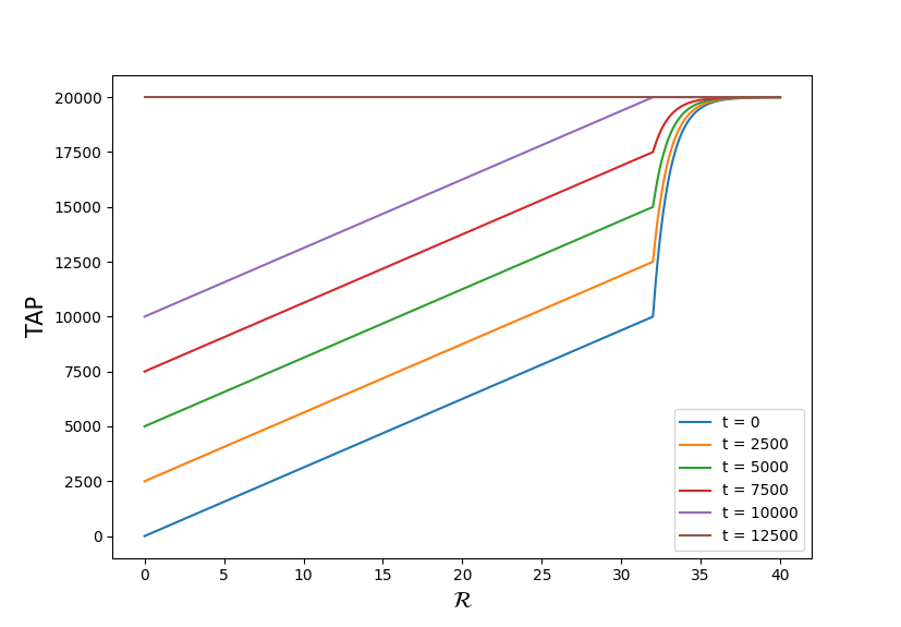
Figure 1: Variation in TAP with $\mathcal{R}$ for constant t (best viewed in color)

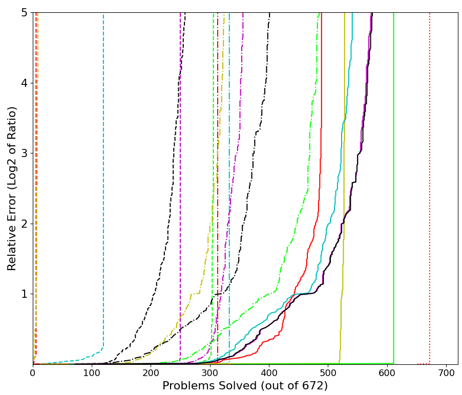
(a) Relative error

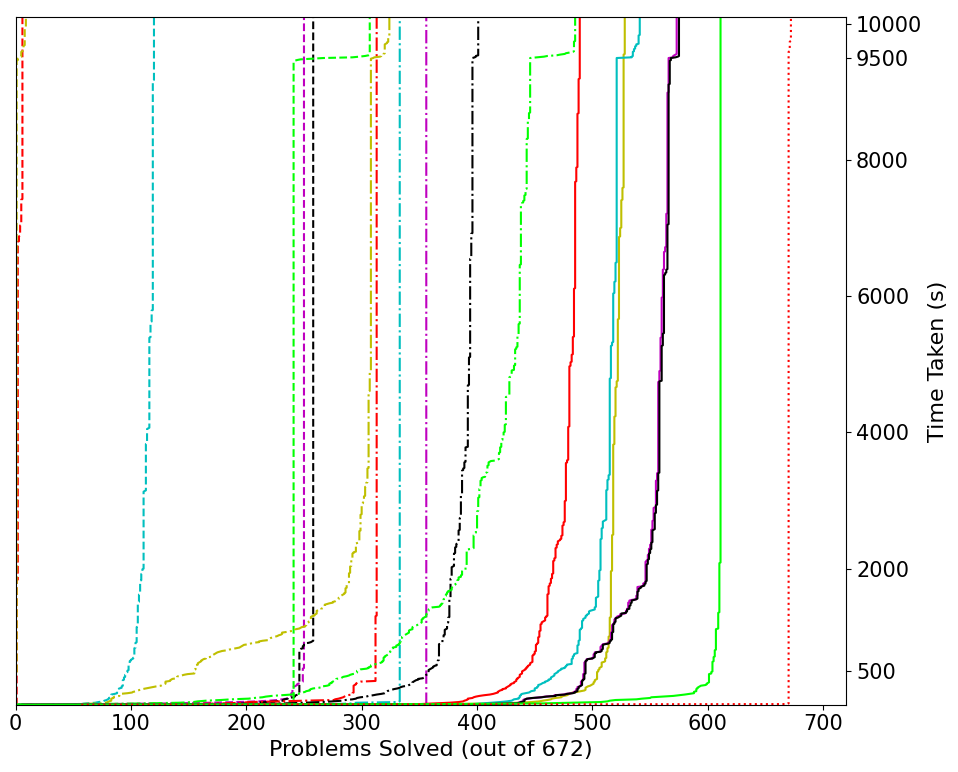
(b) Time taken

Figure 2: Cactus plots (best viewed in color)

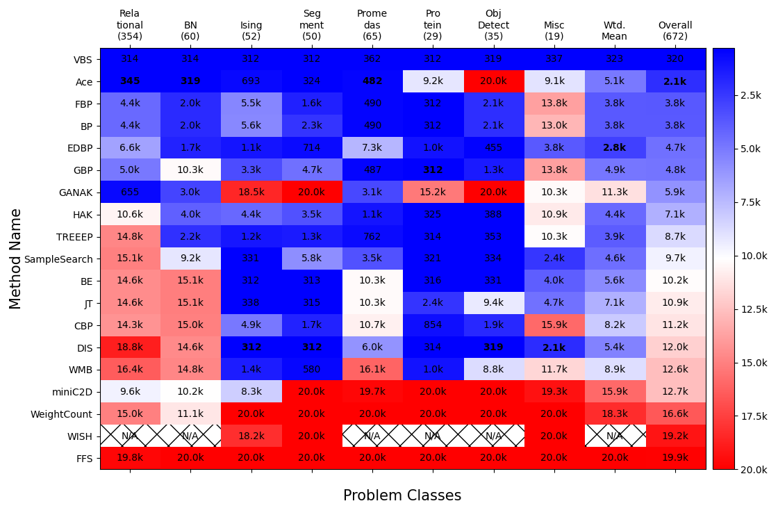
Figure 3: TAP score heatmap - method $\times$ problem class

5 Experimental Evaluation

The experimental evaluation was conducted on a supercomputing cluster provided by NSCC, Singapore. Each experiment consisted of running a tool on a particular benchmark on a 2.60GHz core with a memory limit of 4 GB. The objective of our experimental evaluation was to measure empirical performance of techniques along the Benchmarks Solved, Runtime Variation, Accuracy and TAP score.

5.1 Benchmarks

Table 2 presents a characterization of the graphical models employed in the evaluation on the number of variables ($|\mathbf{X}|$), the number of factors ($|\mathbf{S}|$), the cardinality of variables, and the scope size of factors. The evidences (if any) were incorporated into the model itself by adding one factor per evidence. This step is necessary for a fair comparison with methods that use .cnf since they do not take evidence as a separate parameter.

Different implementations and libraries accepted graphical models in different formats: Merlin, DIS, SampleSearch, Ace and WISH used the .uai format; libDAI used .fg files obtained using a converter in libDAI; WeightCount, miniC2D and GANAK used weighted .cnf files obtained using a utility in Ace’s implementation; FocusedFlatSAT used unweighted .cnf files.

5.2 Reliable Algorithms

To obtain $\hat{Z}$ for 672 benchmarks as described in Section 4, the reliable algorithms chosen were Bucket Elimination and miniC2D.

$Z$ computed by Ace and Junction Tree algorithm agree with each other in all the cases when they both return an answer, i.e. the log₂ of their outputs are identical upto three decimal places. To verify the robustness of computing $\hat{Z}$ using reliable algorithms, we focus on the benchmarks where we can calculate both the true $Z$ and the median of the outputs of reliable algorithms. For such benchmarks, the log₂ of two values are identical upto three decimal places in $99.3\%$ cases. This implies that by computing $\hat{Z}$ using the approach defined in 4.1, the dataset can be extended effectively and reliably.

5.3 Implementation Details

The implementations of all Message Passing Algorithms except Iterative Join Graph Propagation and Edge Deletion Belief Propagation are taken from libDAI Mooij (2010). The library Merlin implements Bucket Elimination and Weighted Mini Bucket Elimination Marinescu (2019). The tolerance was set to $0.001$ in libDAI and Merlin wherever applicable, which is a measure of how small the updates can be in successive iterations, after which the algorithm is said to have converged. For the rest of the methods, implementations provided by respective authors have been used. The available implementation of WISH supports the computation of $Z$ over factor graphs containing unary/binary variables and factors only.

5.4 Results

We include the results of a Virtual Best Solver (VBS) in our comparisons. A VBS is a hypothetical solver that performs as well as the best performing method for each benchmark.

5.4.1 Benchmarks Solved

Table 1 describes the number of problems solved within a 32-factor accuracy. Abbreviations for the methods are mentioned in parentheses that are also used in the results below. To handle cases when a particular algorithm returns a highly inaccurate estimate of $Z$ before the timeout, we consider a problem solved by a particular algorithm only if the value returned is different from the $\hat{Z}$ by a factor of at most 32.

Ace solves the maximum number of problems, followed by Loopy and Fractional Belief Propagations. In problem classes with larger variable cardinality, BP and FBP solve more problems than Ace. Other methods that exactly compute the partition function solve significantly fewer problems as compared to Ace.

5.4.2 Accuracy

Figure 2(a) shows the cactus plot comparing relative errors of algorithms. A curve passing through $(x,y)$ implies that the corresponding method could solve $x$ problems with a relative error of less than $2^{y}$. The curves of the reliable algorithms, as defined in Section 4, are vertical lines as expected, and its X-intercept is a measure of the number of problems solved.

On the other hand, BP and its variants have curves that advance relatively smoothly. This is because these methods cannot provide guarantees for graphical models that do not have a tree-like structure. It should be noted that Ace not only returns the exact values of the partition function but also solves the maximum number of benchmarks amongst all algorithms under a 32-factor accuracy restriction.

From the VBS graph, it can be inferred that every problem in the set of benchmarks can be solved with a relative error of less than $2^{0.01}$ by at least one of the methods.

5.4.3 Runtime Variation

Figure 2(b) shows the cactus plot comparing the time taken by different methods. If a curve passes through $(x,y)$, it implies that the corresponding method could solve $x$ problems with a 32-factor accuracy in not more than $y$ time. The break in the curves at 9500 seconds is due to the soft timeout, and the problems solved after that point have returned an answer within 32-factor accuracy based on incomplete execution.

Vertical curves, such as those of SampleSearch and Bucket Elimination, indicate that these methods either return an answer in a short time or do not return an answer at all for most benchmarks. According to the VBS data, all problems can be solved with a 32-factor accuracy in $<$20 seconds by at least one method. Furthermore, For 670 out of 672 problems, there exists at least one method that can solve the given problem with relative error less than $2^{0.01}$ in time less than 500 seconds.

5.4.4 TAP Score

We plot a heatmap of the TAP score of the algorithms over problem classes in Figure 3. ‘Wtd. Mean’ assigns equal weight to each problem class despite its size, whereas ‘Overall’ takes the average of TAP score over all the problems. If method $m$ has the lowest TAP score for a problem class $c$, it is indicated in bold on the heatmap. If this minimum TAP score is comparable to the corresponding score for VBS, it implies that method $m$ performs better than its counterparts on most problems in class $c$. For instance, in ObjDetect class, DIS has a performance comparable to the Virtual Best Solver.

Despite the lack of formal guarantees, Belief Propagation and its variants have a low overall TAP score, and a relatively consistent performance across all classes. Thus, BP is the best candidate to perform inference on an assorted dataset if formal guarantees are unnecessary. Among the exact methods, Ace performs significantly better than others, and it should be preferred for exact inference.

GANAK, a counting-based method performs well on Relational, Promedas, and BN problems that have a higher factor scope size on an average. However, its TAP scores on the classes with a lower factor scope size such as Ising, Segment, ObjDetect, and Protein is high, signaling a poor performance. The opposite is valid for a subset of methods that do not use model counting, i.e., they perform well on classes with a smaller factor scope size. The methods that show such behavior are JT, BE, and DIS.

5.5 Limitations and Threats to Validity

The widespread applications of the partition function estimation problem have prompted the development of a substantial number of algorithms and their modifications that employ various input formats and implementation methods. The sheer diversity makes it impossible to conduct an exhaustive, impartial study of all the available approaches.

To name a few, the K* method Lilien et al. (2005), the A* algorithm Leach and Lemon (1998), and a method using randomly perturbed MAP solvers Hazan and Jaakkola (2012) have not been compared due to the unavailability of a suitable implementation. Also, of note are the recently proposed techniques for weighted model counting that have shown to perform well in the model counting competition Fichte et al. (2020). Likewise, benchmarks that could not be converted into compatible formats were not included in the study.

6 Concluding Remarks and Outlook

Several observations are in order based on the extensive empirical study: First, observe that the VBS has a mean TAP score an order of magnitude lower than the best solver. Such an observation in the context of SAT solving led to an exciting series of works on the design of portfolio solvers Hutter et al. (2007); Xu et al. (2008). In this context, it is worth highlighting that for every problem, at least one method was able to solve in less than 20 seconds with a 32-factor accuracy. Also, for every benchmark, there existed a technique that could compute an answer with a relative error less than $2^{0.01}$ in $<$500 seconds.

Secondly, model counting-based exact techniques are as competitive as techniques without guarantees on the quality of estimates. Coupled with the surprisingly weak performance of approximate techniques, we believe that there is an exciting opportunity for the development of techniques that scale better than exact techniques.

Finally, the notion of TAP score introduced in this paper allows us to compare approximate techniques by considering both the estimate quality and the runtime performance. We have made the empirical data public, and we invite the community to perform a detailed analysis of the behavior of techniques in the context of structural parameters such as treewidth, the community structure of incidence and primal graphs, and the like.

References

- Agrawal et al. [2020] D. Agrawal, Bhavishya, and K. S. Meel. On the sparsity of xors in approximate model counting. In SAT, 2020.
- Amari et al. [2001] S. Amari, S. Ikeda, and H. Shimokawa. Information geometry of -projection in mean field approximation. Advanced Mean Field Methods - Theory and Practice, 2001.
- Broka et al. [2018] Filjor Broka, Rina Dechter, Alexander Ihler, and Kalev Kask. Abstraction sampling in graphical models. In UAI, 2018.
- Chakraborty et al. [2015] S. Chakraborty, D. Fried, K. S. Meel, and M. Y. Vardi. From weighted to unweighted model counting. In IJCAI, 2015.
- Chavira and Darwiche [2005] M. Chavira and A. Darwiche. Compiling bayesian networks with local structure. In IJCAI, 2005.
- Chavira and Darwiche [2007] M. Chavira and A. Darwiche. Compiling bayesian networks using variable elimination. In IJCAI, 2007.
- Chavira and Darwiche [2008] M. Chavira and A. Darwiche. On probabilistic inference by weighted model counting. Artificial Intelligence, 2008.
- Chavira et al. [2004] M. Chavira, A. Darwiche, and M. Jaeger. Compiling relational bayesian networks for exact inference. International Journal of Approximate Reasoning, 2004.
- Choi and Darwiche [2006] A. Choi and A. Darwiche. An edge deletion semantics for belief propagation and its practical impact onapproximation quality. In AAAI, 2006.
- Cundy and Ermon [2020] C. Cundy and S. Ermon. Flexible approximate inference via stratified normalizing flows. In UAI, 2020.
- Darwiche and Marquis [2002] Adnan Darwiche and Pierre Marquis. A knowledge compilation map. Journal of Artificial Intelligence Research, 2002.
- Darwiche [1995] A. Darwiche. Conditioning algorithms for exact and approximate inference in causal networks. In UAI, 1995.
- Darwiche [2001a] A. Darwiche. On the tractable counting of theory models and its application to truth maintenance and belief revision. JANCL, 2001.
- Darwiche [2001b] A. Darwiche. Recursive conditioning. Artificial Intelligence, 2001.
- Darwiche [2002] A. Darwiche. A logical approach to factoring belief networks. KR, 2002.
- Darwiche [2004] A. Darwiche. New advances in compiling CNF into decomposable negation normal form. In ECAI, 2004.
- Darwiche [2009] A. Darwiche. Modeling and reasoning with bayesian networks, 2009.
- Darwiche [2011] A. Darwiche. SDD: A new canonical representation of propositional knowledge bases. In IJCAI, 2011.
- de Colnet and Meel [2019] A. de Colnet and K. S. Meel. Dual hashing-based algorithms for discrete integration. In CP, 2019.
- Dechter et al. [2002] R. Dechter, K. Kask, and R. Mateescu. Iterative join-graph propagation. In UAI, 2002.
- Dechter [1996] R. Dechter. Bucket elimination: A unifying framework for probabilistic inference. In UAI, 1996.
- Dechter [1999] R. Dechter. Bucket elimination: A unifying framework for reasoning, 1999.
- Doucet et al. [2000] A. Doucet, N. de Freitas, K. P. Murphy, and S. J. Russell. Rao-blackwellised particle filtering for dynamic bayesian networks. In UAI, 2000.
- Dudek et al. [2020] J. M. Dudek, D. Fried, and K. S. Meel. Taming discrete integration via the boon of dimensionality. In NeurIPS, 2020.
- Eaton and Ghahramani [2009] F. Eaton and Z. Ghahramani. Choosing a variable to clamp. In AISTATS, 2009.
- Ermon et al. [2011] S. Ermon, C. Gomes, A. Sabharwal, and B. Selman. Accelerated adaptive markov chain for partition function computation. In NIPS, 2011.
- Ermon et al. [2013a] S. Ermon, C. Gomes, A. Sabharwal, and B. Selman. Optimization with parity constraints: From binary codes to discrete integration. In UAI, 2013.
- Ermon et al. [2013b] S. Ermon, C. Gomes, A. Sabharwal, and B. Selman. Taming the curse of dimensionality: Discrete integration by hashing and optimization. In ICML, 2013.
- Fan and Fan [2008] X. Fan and G. Fan. Graphical models for joint segmentation and recognition of license plate characters. IEEE Signal Processing Letters, 2008.
- Fichte et al. [2020] Johannes K Fichte, Markus Hecher, and Florim Hamiti. The model counting competition 2020. arXiv preprint arXiv:2012.01323, 2020.
- Georgiev et al. [2012] I. Georgiev, R. H. Lilien, and B. R. Donald. The minimized dead-end elimination criterion and its application to protein redesign in a hybrid scoring and search algorithm for computing partition functions over molecular ensembles. Journal of Computational Chemistry, 2012.
- Gillespie [2013] D. Gillespie. Computing the partition function, ensemble averages, and density of states for lattice spin systems by sampling the mean. Journal of Computational Physics, 2013.
- Gogate and Dechter [2005] V. Gogate and R. Dechter. Approximate inference algorithms for hybrid bayesian networks with discrete constraints. In UAI, 2005.
- Gogate and Dechter [2011] V. Gogate and R. Dechter. Samplesearch: Importance sampling in presence of determinism. Artificial Intelligence, 2011.
- Grover et al. [2018] Aditya Grover, Tudor Achim, and Stefano Ermon. Streamlining variational inference for constraint satisfaction problems. In NeurIPS, 2018.
- Hazan and Jaakkola [2012] T. Hazan and T. Jaakkola. On the partition function and random maximum a-posteriori perturbations. In ICML, 2012.
- Henrion [1988] M. Henrion. Propagating uncertainty in bayesian networks by probalistic logic sampling. In UAI, 1988.
- Heskes et al. [2003] T. Heskes, C. A. Albers, and H. J. Kappen. Approximate inference and constrained optimization. In UAI, 2003.
- Heule et al. [2019] Marijn JH Heule, Matti Jarvisalo, and Martin Suda. Sat competition 2018. Journal on Satisfiability, Boolean Modeling and Computation, 2019.
- Horvitz et al. [1989] E. J. Horvitz, H. J. Suermondt, and G. Cooper. Bounded conditioning: Flexible inference for decisions under scarce resources. In UAI, 1989.
- Hutter et al. [2007] Frank Hutter, Holger H. Hoos, and Thomas Stutzle. Automatic algorithm configuration based on local search. In AAAI, 2007.
- Jensen et al. [1990] F. V. Jensen, S. L. Lauritzen, and K. G. Olesen. Bayesian updating in causal probabilistic networks by local computation. Computational Statistics Quarterly, 1990.
- Jerrum and Sinclair [1993] M. Jerrum and A. Sinclair. Polynomial-time approximation algorithms for the ising model. SIAM Journal on Computing, 1993.
- Koller and Friedman [2009] D. Koller and N. Friedman. Probabilistic graphical models: Principles and techniques, 2009.
- Kschischang et al. [2001] F. Kschischang, B. Frey, and H. A. Loeliger. Factor graphs and the sum-product algorithm. IEEE TIT, 2001.
- Kuck et al. [2018] J. Kuck, A. Sabharwal, and S. Ermon. Approximate inference via weighted rademacher complexity. In AAAI, 2018.
- Kuck et al. [2019] J. Kuck, T. Dao, S. Zhao, B. Bartan, A. Sabharwal, and S. Ermon. Adaptive hashing for model counting. In UAI, 2019.
- Kuck et al. [2020] Jonathan Kuck, Shuvam Chakraborty, Hao Tang, Rachel Luo, Jiaming Song, Ashish Sabharwal, and Stefano Ermon. Belief propagation neural networks. In NeurIPS, 2020.
- Lagniez and Marquis [2017] J. Lagniez and P. Marquis. An improved decision-DNNF compiler. In IJCAI, 2017.
- Lagniez and Marquis [2019] Jean-Marie Lagniez and Pierre Marquis. A recursive algorithm for projected model counting. In AAAI, 2019.
- Lauritzen and Spiegelhalter [1988] S. L. Lauritzen and D. J. Spiegelhalter. Local computation with probabilities on graphical structures and their application to expert systems. Journal of the Royal Statistical Society, Series B, 1988.
- Leach and Lemon [1998] A. Leach and A. Lemon. Exploring the Conformational Space of Protein Side Chains Using Dead-end Elimination and the A* Algorithm. Proteins, 1998.
- Lee et al. [2019] J. Lee, R. Marinescu, A. Ihler, and R. Dechter. A weighted mini-bucket bound for solving influence diagrams. In UAI, 2019.
- Lilien et al. [2005] R. Lilien, B. Stevens, A. Anderson, and BR Donald. A novel ensemble-based scoring and search algorithm for protein redesign, and its application to modify the substrate specificity of the gramicidin synthetase a phenylalanine adenylation enzyme. Journal of Computational Biology, 2005.
- Liu and Ihler [2011] Q. Liu and A. T. Ihler. Bounding the partition function using Holder’s inequality. In ICML, 2011.
- Liu et al. [2015] Qiang Liu, Jian Peng, Alexander Ihler, and John Fisher III. Estimating the partition function by discriminance sampling. In UAI, 2015.
- Lou et al. [2017] Q. Lou, R. Dechter, and A. Ihler. Dynamic importance sampling for anytime bounds of the partition function. In NIPS, 2017.
- Ma et al. [2013] Jianzhu Ma, Jian Peng, Sheng Wang, and Jinbo Xu. Estimating the partition function of graphical models using langevin importance sampling. In AISTATS, 2013.
- Marinescu [2019] R. Marinescu. Merlin: An extensible C++ library for probabilistic inference over graphical models, 2019.
- Mateescu and Dechter [1990] R. Mateescu and R. Dechter. Axioms for probability and belief-function propagation. In UAI, 1990.
- Mateescu and Dechter [2005] R. Mateescu and R. Dechter. And/or cutset conditioning. In IJCAI, 2005.
- McCallum et al. [2009] A. McCallum, K. Schultz, and S. Singh. FACTORIE: Probabilistic programming via imperatively defined factor graphs. In NIPS, 2009.
- Meel and Akshay [2020] K. S. Meel and S. Akshay. Sparse hashing for scalable approximate model counting: Theory and practice. In LICS, 2020.
- Minka [2001] P. Minka. A family of algorithms for approximate bayesian inference, PhD Thesis, MIT Cambridge, 2001.
- Molkaraie and Loeliger [2012] M. Molkaraie and H. A. Loeliger. Monte carlo algorithms for the partition function and information rates of two-dimensional channels. IEEE TIT, 2012.
- Mooij [2010] J. M. Mooij. libDAI: A free and open source C++ library for discrete approximate inference in graphical models. Journal of Machine Learning Research, 2010.
- Murphy [2012] K. P. Murphy. Machine learning: a probabilistic perspective, 2012.
- Oztok and Darwiche [2015] U. Oztok and A. Darwiche. A top-down compiler for sentential decision diagrams. In IJCAI, 2015.
- Pabbaraju et al. [2020] C. Pabbaraju, P. Wang, and J. Z. Kolter. Efficient semidefinite-programming based inference for binary and multi class mrfs. In NeurIPS, 2020.
- Pearl [1982] J. Pearl. Reverend Bayes on Inference Engines: A Distributed Hierarchical Approach. In AAAI, 1982.
- Pearl [1986] J. Pearl. A constraint-propagation approach to probabilistic reasoning. In UAI, 1986.
- Pearl [1988] J. Pearl. Probabilistic Reasoning in Intelligent Systems: Networks of Plausible Inference. 1988.
- Peyrard et al. [2019] N. Peyrard, M.-J. Cros, S. de Givry, A. Franc, S. Robin, R. Sabbadin, T. Schiex, and M. Vignes. Exact or approximate inference in graphical models: why the choice is dictated by the treewidth, and how variable elimination can be exploited. ANZJS, 2019.
- Qi and Minka [2004] Y. Qi and T. Minka. Tree-structured approximations by expectation propagation. In NIPS, 2004.
- Roth [1996] D. Roth. On the hardness of approximate reasoning. Artificial Intelligence, 1996.
- Saeedi et al. [2017] Ardavan Saeedi, Tejas D Kulkarni, Vikash K Mansinghka, and Samuel J Gershman. Variational particle approximations. JMLR, 2017.
- Shachter and Peot [1989] R. Shachter and M. Peot. Simulation approaches to general probabilistic inference on belief networks. In UAI, 1989.
- Sharma et al. [2019] S. Sharma, S. Roy, M. Soos, and K. S. Meel. GANAK: A scalable probabilistic exact model counter. In IJCAI, 2019.
- Shu et al. [2018] Rui Shu, Hung Bui, Shengjia Zhao, Mykel Kochenderfer, and Stefano Ermon. Amortized inference regularization. In NeurIPS, 2018.
- Shu et al. [2019] Rui Shu, Hung Bui, Jay Whang, and Stefano Ermon. Training variational autoencoders with buffered stochastic variational inference. In AISTATS, 2019.
- Soos and Meel [2019] M. Soos and K. S. Meel. Bird: Engineering an efficient CNF-XOR SAT solver and its applications to approximate model counting. In AAAI, 2019.
- Soos et al. [2020] M. Soos, S. Gocht, and K. S. Meel. Tinted, detached, and lazy cnf-xor solving and its applications to counting and sampling. In CAV, 2020.
- Thurley [2006] M. Thurley. sharpSAT - counting models with advanced component caching and implicit bcp. In SAT, 2006.
- Viricel et al. [2016] C. Viricel, D. Simonichi, S. Barbe, and T. Schiex. Guaranteed weighted counting for affinity computation: Beyond determinism and structure. In CP, 2016.
- Wainwright et al. [2001] M. J. Wainwright, T. Jaakkola, and A. S. Willsky. Tree-based reparameterization for approximate inference on loopy graphs. In NIPS, 2001.
- Waldorp and Marsman [2019] Lourens Waldorp and Maarten Marsman. Intervention in undirected ising graphs and the partition function. forthcoming, 2019.
- Wiegerinck and Heskes [2003] W. Wiegerinck and T. Heskes. Fractional belief propagation. In NIPS, 2003.
- Winkler [2002] G. Winkler. Image Analysis, Random Fields and Markov Chain Monte Carlo Methods: A Mathematical Introduction. 2002.
- Wu et al. [2019] Mike Wu, Noah Goodman, and Stefano Ermon. Differentiable antithetic sampling for variance reduction in stochastic variational inference. In AISTATS, 2019.
- Wu et al. [2020] Mike Wu, Kristy Choi, Noah Goodman, and Stefano Ermon. Meta-amortized variational inference and learning. In AAAI, 2020.
- Xu et al. [2008] Lin Xu, Frank Hutter, Holger H. Hoos, and Kevin Leyton-Brown. Satzilla: Portfolio-based algorithm selection for SAT. Journal of Artificial Intelligence Research, 2008.
- Yedidia et al. [2000] J. S. Yedidia, W. T. Freeman, and Y. Weiss. Generalized belief propagation. In NIPS, 2000.
- Zeng et al. [2020] Z. Zeng, P. Morettin, F. Yan, A. Vergari, and G. Van den Broeck. Probabilistic inference with algebraic constraints: Theoretical limits and practical approximations. In NeurIPS, 2020.
- Zhang and Poole [1994] N. L. Zhang and D. Poole. A simple approach to bayesian network computations. In UAI, 1994.