Partial synchronization in the Kuramoto model with attractive and repulsive interactions via the Bellerophon state

Abstract

We study two groups of nonidentical Kuramoto oscillators with differing frequency distributions. Coupling between the groups is repulsive, while coupling between oscillators of the same group is attractive. This asymmetry of interactions leads to an interesting synchronization behavior. For small coupling strength, the mean-fields of both groups resemble a more weakly coupled Kuramoto model. After increasing the coupling strength beyond a threshold, they reach the Bellerophon state of multiple clusters of averagely entrained oscillators. A further increase in the coupling strength then asymptotically transitions from the Bellerophon state to a single synchronized cluster. During this transition, the order parameters of both groups increase and resemble an equally strongly coupled Kuramoto model. Our analysis is based on the Ott-Antonsen mean-field theory.

I Introduction

Synchronization describes the emergence of a common mode in a system of interacting units. It has been observed in many different contexts, such as power grids Motter et al. (2013), neuronal populations Uhlhaas (2009), or the synchronization of pedestrians on a bridge Strogatz et al. (2005). One of the most popular models in the study of synchronization is the Kuramoto model Kuramoto (1984); Acebrón et al. (2005); Pikovsky and Rosenblum (2015). It is widely used for its description of the transition to synchronization and its analytical solvability Watanabe and Strogatz (1993, 1994); Ott and Antonsen (2008, 2009); Mihara and Medrano-T (2019). In the model, only attractive pairwise interactions are considered. However, there exist many systems that contain both attractive and repulsive interactions Peyrache et al. (2012).

A method to model these mixed-interaction systems is the splitting of the oscillator population into two groups. In a conformists-contrarian model, the conformists interact attractively with all oscillators, and the contrarians repulsively Hong and Strogatz (2011a, b); Hong (2014); Qiu et al. (2016). One possible state in such a system with non-identical oscillators is the Bellerophon state Qiu et al. (2016). In this state, clusters exist, where oscillators share the same average frequency but not the same phase or instantaneous frequencies. The clusters have a constant difference in their average frequency, yielding a step-like picture. Oscillators between the clusters behave quasiperiodically.

Each oscillator in such a model of conformists and contrarians has one type of interaction. Another possibility is to differentiate between groups in a model with attractive and repulsive interactions Montbrió, Kurths, and Blasius (2004); Sheeba et al. (2008); Anderson et al. (2012); Hong and Strogatz (2012); Laing (2012); Lohe (2014); Sonnenschein et al. (2015); Pietras, Deschle, and Daffertshofer (2016); Kotwal, Jiang, and Abrams (2017); Achterhof and Meylahn (2021a, b). Typically in this case, each oscillator acts attractively on all oscillators of the same group and repulsively on oscillators of the other group. This model is a very simplified representation of a two-party dynamic, where people in the same party try to agree but at the same time distance themselves from the other party.

This paper considers such a model with attractive and repulsive interaction with independent frequency distributions of the oscillators. For small coupling strength, the macroscopic dynamics of each group resemble the ones of a Kuramoto model with a weaker coupling. The macroscopic frequencies of both groups are entrained, and there exists one entrained cluster. An increase in the coupling strength destroys the entrainment, and the oscillators begin to form loose clusters with a constant average frequency, separated by quasiperiodic ones; they reach a Bellerophon state. A further increase in the coupling strength leads to a jump in the synchronization of each group and an entrainment of both groups’ macroscopic dynamics. The entrained clusters then still exist but start to collapse and approach one big entrained cluster, like the one expected for the Kuramoto model without groups. The observed Bellerophon state is very susceptible to changes in the frequency distribution.

The paper is organized as follows. First, the model is introduced. The solution for the mean-field in the thermodynamic limit is then found with the Ott-Antonsen Ansatz. Using the Ott-Antonsen equations, the mean-field dynamics are investigated for increasing coupling strength, and the behavior is compared to the Kuramoto model. Finally, the findings are summarized.

II The model

The standard Kuramoto model Kuramoto (1984); Acebrón et al. (2005) only considers a single group of nonidentical oscillators. To describe a system of $M$ interacting groups, the M-Kuramoto model Qiu et al. (2016); Maistrenko, Penkovsky, and Rosenblum (2014) is needed. It is defined as

$$\dot{\theta}^{\sigma}_{j}=\omega^{\sigma}_{j}+\sum_{\sigma^{\prime}=1}^{M}\frac{K_{\sigma\sigma^{\prime}}}{N}\sum_{k=1}^{N_{\sigma^{\prime}}}\sin(\theta^{\sigma^{\prime}}_{k}-\theta^{\sigma}_{j})\;.$$ (1)

Here $\omega^{\sigma}_{j}$ is the natural frequency of the $j$th oscillator in group $\sigma$ and $K_{\sigma\sigma^{\prime}}$ is the coupling strength between groups $\sigma$ and $\sigma^{\prime}$. Every group consists of $N_{\sigma}$ oscillators with a total system size of $N=\sum_{\sigma^{\prime}}N_{\sigma^{\prime}}$. In a simple model with attractive and repulsive interactions, there are only two groups. To further simplify this, we consider equal intra-coupling and inter-coupling $K_{\sigma\sigma^{\prime}}=2K$ if $\sigma=\sigma^{\prime}$ and $K_{\sigma\sigma^{\prime}}=-2K$ else, respectively, and equally sized groups $N_{1}=N_{2}$. For the sake of analytical tractability, the oscillators’ natural frequencies are chosen from a Lorentzian distribution $g(\omega)$

$$g(\omega)=\frac{1}{\pi\gamma\left[1+\left(\frac{\omega-\bar{w}}{\gamma}\right)^{2}\right]}\;,$$ (2)

where both groups have different centers $\bar{w}$ and widths $\gamma$. By rotating the reference frame, the first group can be centered at $\bar{\omega}_{1}=0$, and by scaling of the time, the width of the first group can be set to $\gamma_{1}=0.1$. Without loss of generality, the first group is always chosen to be the narrower one, i.e., $\gamma_{2}\geq 0.1$. This model can also be represented as a single group but with a bimodal frequency distribution and one additional bifurcation parameter Pietras, Deschle, and Daffertshofer (2016).

Introducing the mean field for each group $Z_{\sigma}=R_{\sigma}e^{i\Theta_{\sigma}}=(1/N_{\sigma})\sum_{k}e^{i\theta^{\sigma}_{k}}$ and renaming $\theta^{1}_{j}=\varphi_{j}$ and $\theta^{2}_{j}=\psi_{j}$ yields the system

$$\dot{\varphi}_{j}= \omega_{1,j}+KR_{1}\sin(\Theta_{1}-\varphi_{j})-KR_{2}\sin(\Theta_{2}-\varphi_{j})\;,$$ (3)

$$\dot{\psi}_{j}= \omega_{2,j}-KR_{1}\sin(\Theta_{1}-\psi_{j})+KR_{2}\sin(\Theta_{2}-\psi_{j})\;.$$

Note that $K=K_{\sigma\sigma^{\prime}}/2$, so the coupling strength of each group is halved compared to the M-Kuramoto model. From there, the forcing $H$ for each group can be determined to be

$$H_{\sigma}=h_{\sigma}e^{i\Phi_{\sigma}}=K(Z_{\sigma}-Z_{\sigma^{\prime}})\;,$$ (4)

where $\sigma^{\prime}$ denotes the other group. Both forcings are connected via $H_{2}=-H_{1}$, so their magnitudes are identical, $h_{1}=h_{2}=h$, and they are just shifted by a phase $\Phi_{1}=\Phi=\Phi_{2}-\pi$. The forced equations for the oscillators are then

$$\dot{\varphi}_{j}= \omega_{1,j}+\mbox{Im}\left[H_{1}e^{-i\varphi_{j}}\right]=\omega_{1,j}+h\sin(\Phi-\varphi_{j})\;,$$ (5)

$$\dot{\psi}_{j}= \omega_{2,j}+\mbox{Im}\left[H_{2}e^{-i\psi_{j}}\right]=\omega_{2,j}+h\sin(\Phi-\psi_{j}+\pi)\;.$$

II.1 Thermodynamic limit

Systems consisting of the imaginary part of a forcing, like Eqs. (5) separately, have an analytical description of their mean-field in the thermodynamic limit. The mean-field evolution is found with the Ott-Antonsen (OA) Ansatz Ott and Antonsen (2008, 2009); Pikovsky and Rosenblum (2008) and in the case of a Lorentzian distribution of the frequencies $\omega$ the mean-field dynamics in the OA Ansatz are  Pazó and Gallego (2020)

$$\dot{Z}=(-\gamma+i\bar{\omega})Z+\frac{1}{2}(H-H^{*}Z^{2})\;,$$ (6)

with $H^{*}$ being the complex conjugate of $H$. By using the definition of the forcing in Eq. (4) this becomes

$$\dot{Z}_{\sigma}=(-\gamma_{\sigma}+i\bar{\omega}_{\sigma})Z_{\sigma}+\frac{K}{2}(Z_{\sigma}(1-R_{\sigma}^{2}+Z^{*}_{\sigma^{\prime}}Z_{\sigma})-Z_{\sigma^{\prime}})\;.$$ (7)

Calculating the derivative of the mean-field $\dot{Z}_{\sigma}=\dot{R}_{\sigma}e^{i\Theta_{\sigma}}+iR_{\sigma}\dot{\Theta}_{\sigma}e^{i\Theta_{\sigma}}$, multiplying Eq. (7) by $e^{-i\Theta_{\sigma}}$ and splitting the real and imaginary part yields the dynamics of the order parameter and the phase of the mean-field as

$$\dot{R}_{\sigma}= -\gamma_{\sigma}R_{\sigma}+\frac{K}{2}(1-R_{\sigma}^{2})(R_{\sigma}-R_{\sigma^{\prime}}\cos(\Theta_{\sigma}-\Theta_{\sigma^{\prime}}))\;,$$ (8)

$$\dot{\Theta}_{\sigma}= \bar{\omega}_{\sigma}+\frac{K}{2}\frac{R_{\sigma^{\prime}}}{R_{\sigma}}(1+R_{\sigma}^{2})\sin(\Theta_{\sigma}-\Theta_{\sigma^{\prime}})\;.$$

Both equations only depend on the difference between the mean-field phases, as expected in a rotational invariant system. The 4-dimensional system (order parameter and mean-field phase of each group) can then be reduced to a 3-dimensional system of the order parameters and the phase difference $\Theta=\Theta_{1}-\Theta_{2}$ to

$$\dot{R}_{1}= -\gamma_{1}R_{1}+\frac{K}{2}(1-R_{1}^{2})(R_{1}-R_{2}\cos\Theta)\;,$$ (9)

$$\dot{R}_{2}= -\gamma_{2}R_{2}+\frac{K}{2}(1-R_{2}^{2})(R_{2}-R_{1}\cos\Theta)\;,$$

$$\dot{\Theta}= -\bar{\omega}_{2}+\frac{K}{2}\sin\Theta\frac{R_{1}^{2}(R_{2}^{2}+1)+R_{2}^{2}(R_{1}^{2}+1)}{R_{1}R_{2}}\;.$$

Indicator oscillators can be used to study the system in the thermodynamic limit. They are coupled to the OA mean-fields from Eqs. (8) but do not create a mean-field themselves. From Eqs. (5), the same forcing acts on both groups, so their dynamics will be equal for the same $\omega_{j}$ up to the phase shift. The dynamics of a single indicator oscillator depends only on the oscillator’s frequency, not on the group it belongs to. To discern the phases of indicator oscillators, they are marked as $\theta^{\prime}_{j}$ with their natural frequencies $\omega^{\prime}_{j}$. They follow the equations (we choose to consider them as part of group 2)

$$\dot{\theta}^{\prime}_{j}=\omega^{\prime}_{j}-KR_{1}\sin(\Theta_{1}-\theta^{\prime}_{j})+KR_{2}\sin(\Theta_{2}-\theta^{\prime}_{j})\;.$$ (10)

The $R_{1,2}$ and $\Theta_{1,2}$ are calculated from Eq. (8), and the $\omega^{\prime}$ are chosen uniformly. This method makes it possible to calculate the observed frequencies $\dot{\theta}^{\prime}$ and the phase distribution in the thermodynamic limit numerically.

III Small coupling strength

In the Kuramoto model, i.e., Eq. (1) with $M=1$, the critical coupling for the emergence of a nonzero order parameter and the function $\hat{R}(\hat{K})$ is known analytically in the case of a Lorentzian distribution of the phases Acebrón et al. (2005). The critical coupling for the transition from incoherence to partial synchrony is

$$\hat{K}_{c}=2\hat{\gamma}\;,$$ (11)

and the order parameter

$$\hat{R}=\sqrt{1-\frac{\hat{K_{c}}}{\hat{K}}}\;.$$ (12)

The hat notation ,$\hat{K}$, marks the quantities of the Kuramoto model.

In the considered model with $M=2$, if both groups are identical, then the critical coupling strength of each group corresponds to the Kuramoto model’s one Anderson et al. (2012). To compare the nontrivial order parameter between the Kuramoto model in Eq. (12) and the model with attractive and repulsive interactions in Eq. (7), the coupling constants have to be scaled, as $K_{\sigma\sigma^{\prime}}=2K$ was chosen and in the case of the Kuramoto model $K_{\sigma\sigma^{\prime}}=\hat{K}$, so $\hat{K}=2K$. A comparable critical coupling $K_{c}$ for the contrarian model would then correspond to $K_{c}=2\gamma=4\hat{\gamma}$, i.e., $\gamma=2\hat{\gamma}$. The order parameter will have the same form, as $K_{c}/K$ from Eq. (12) only depends on $K_{c}$.

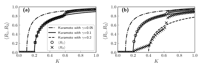
Figure 1: Average order parameters of group 1 $\langle R_{1}\rangle$ as circles and group 2 $\langle R_{2}\rangle$ as crosses. The solid (dashed, dash-dotted) black line shows the average order parameter in a Kuramoto model with $\gamma=0.1$ ($\gamma=0.2$, $\gamma=0.05$). In (a) $\gamma_{2}=0.1$, so both distributions have the same width but different centers, and in (b) $\gamma_{2}=0.2$. The width is $\bar{\omega}_{2}=1$ in both cases.

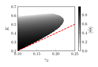
Figure 2: The difference in average frequencies of the mean fields $\langle\dot{\Theta}\rangle$ for $\bar{\omega}_{2}=1$. The red dashed line is the critical coupling of a Kuramoto model with the same width of the frequency distribution $\hat{\gamma}=\gamma$ as the second group in Eq. (11). The critical coupling for group 1 is $K=0.2$, below this the system is incoherent ($R_{1}=R_{2}=0$). For any scaling of $\bar{\omega}_{2}$, this image looks identical, if $K$ and $\gamma_{2}$ scaled with the same factor (only the absolute values of the frequency difference change).

For small coupling strength, both groups are incoherent. In Fig. 1, it is shown that the critical coupling strength for the first group corresponds to $K_{c,1}=0.2$, the same as in a Kuramoto model with $\hat{\gamma}_{1}=\gamma_{1}=0.1$, not the expected $\hat{\gamma}_{1}=\gamma_{1}/2$. The effective coupling strength is only half as strong as in the Kuramoto model. For $K\lessapprox 0.6$, the first group follows the relation in Eq. (12) with $K_{c,1}=0.2$ very well, regardless of $\gamma_{2}$, as can be observed from Fig. 1(a) and (b), when $\gamma_{2}$ changes from $0.1$ to $0.2$. The second group behaves somewhat differently. Its critical coupling follows a perturbed form of $K_{c,2}=2\gamma_{2}$, half as strong as in the Kuramoto model. For $K_{c,1}<K\lessapprox K_{c,2}$ this group is not incoherent but becomes forced by group 1, as shown in Fig. 1(b).

Similar to the Kuramoto model, there exists a cluster of averagely entrained oscillators, centered around $\omega_{j}=0$  with a small shift in the direction of $\bar{\omega}_{2}$. They are entrained to the mean-field of group 1, and, as before, the observed frequency only depends on the oscillator’s natural frequency $\omega_{j}$, not on the group it belongs to . The difference in the groups’ mean-field frequencies can be seen in Fig. 2. The mean-fields are entrained in their average and instantaneous frequency since group 1 forces the, not yet self-synchronized, group 2.

IV Moderate coupling strength

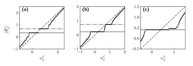
Figure 3: The average observed frequencies of indicator oscillators from Eqs. (8) and (10). The solid (dash-dotted) gray line marks the average mean field frequency $\langle\dot{\Theta}_{1}\rangle$ ($\langle\dot{\Theta}_{2}\rangle$) and the dashed gray line the identity function $\langle\dot{\theta}^{\prime}_{j}\rangle=\omega^{\prime}_{j}$. For all three subfigures $\bar{\omega}_{2}=1$. In (a) $\gamma_{2}=0.1$, $K=0.56$ and identical order parameters $R_{1}=R_{2}$, in (b) $\gamma_{2}=0.2$, $K=0.56$ and $R_{1}\neq R_{2}$, and in (c) $\gamma=0.2$, $K=0.63$ and $R_{1}\neq R_{2}$ but the mean field frequencies are entrained.

With the increase of the coupling strength to $K>K_{c,2}$, new clusters begin to form. These new clusters lead to a stronger synchronization of group 2, and its order parameter better follows the relation Eq. (12) but is smaller than expected, as group 1 perturbs it. The clusters are coherent regions in $\omega$ with a common average frequency, as shown in Fig. 3. Oscillators between the clusters behave quasiperiodically. The entrained clusters decrease in size the further they are from the mean of the two distributions $\bar{\omega}_{2}/2$ , and the two biggest clusters lock to the average frequency of the mean fields (if they are non-entrained). Such a state has been observed in a conformists-contrarian model with a common distribution of frequencies in Ref. Qiu et al. (2016) where they called it the Bellerophon state, noting the difference to the chimera state. There they determined the entrainment frequencies to be uneven multiples of a fundamental frequency. This entrainment to uneven multiples is also the case here, albeit the zero is shifted. In the case of non-entrainment of the mean-fields, the clusters have an average frequency of uneven multiples of the difference in average mean-field frequencies $\Delta\Omega=\langle\dot{\Theta}\rangle/2$ centered around their average mean $\Omega_{0}=(\langle\Theta_{1}\rangle+\langle\Theta_{2}\rangle)/2$, i.e., the frequencies of the clusters $\Omega_{j}$ are

$$\Omega_{\pm(2n+1)}=\Omega_{0}\pm(2n+1)\Delta\Omega\;.$$ (13)

The center frequency $\Omega_{0}$ is not constant but changes with the coupling strength $K$ and $\gamma_{2}$.

The transition between the clusters with $\Omega_{-1}$ and $\Omega_{1}$ depends on $\gamma_{2}$. If both widths $\gamma_{1}=\gamma_{2}$ are identical, then there is a sudden transition between the states (Fig. 3(a)) while for $\gamma_{1}\neq\gamma_{2}$ the transition is smooth(Fig. 3(b)). A similar state has also been observed in Ref.Montbrió, Kurths, and Blasius (2004) for a system of attractive and repulsive oscillators with frequency distributions of common width but different means. The dynamics observed here differ from both, as Ref. Qiu et al. (2016) only considers a conformists-contrarian model and finds only the special case depicted in Fig.3(a) shows a sudden jump between the clusters with frequencies $\Omega_{1}$ and $\Omega_{-1}$. The difference to Ref. Montbrió, Kurths, and Blasius (2004) lies in the perfect overlap of the average frequencies of oscillators with the same $\omega_{j}$, regardless of their group and the different width of the frequency distributions.

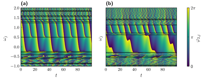
Figure 4: The phases of the indicator oscillators. Approximate cluster borders are marked with black lines. The parameters of (a) and (b) are the same as in Fig. 3 (a) and (b).

The clusters are stable in time, as seen in Fig. 4. While the clusters are fully entrained, they do not share a common phase. The difference in frequency can be seen very well by the additional rotation in the cluster with $\Omega_{1}$ in reference to $\Omega_{-1}$. Again, there is a difference in the case of $\gamma_{1}\neq\gamma_{2}$, where the dynamics have a more complicated phase dynamic.

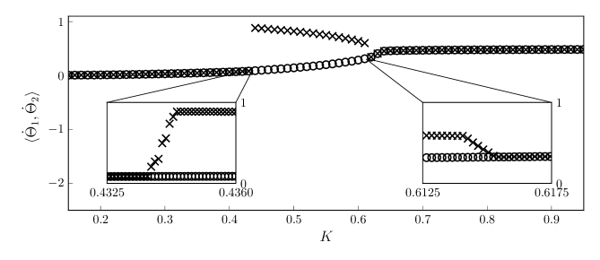
Figure 5: The average frequencies of the mean fields $\langle\dot{\Theta}_{1}\rangle$ (circles) and $\langle\dot{\Theta}_{2}\rangle$ (crosses) for $\bar{\omega}_{2}=1$ and $\gamma_{2}=0.2$. The inset figures show the transition from entrainment to non-entrainment and vice versa. Because the frequency has some very big peaks during the transition, all numerical values with $\left|\dot{\Theta}_{2}\right|>100$ were removed to smoothen the transition.

The Bellerophon state comes into existence before the mean fields lose their entrainment, but after $K_{c,2}$. The clusters lead to the fast transition between entrainment and non-entrainment of the mean-fields in Fig. 5. In the case of $\gamma_{1}=\gamma_{2}$, the forcing $H$ has a unique role. Its average frequency $\langle\dot{\Phi}\rangle$ lies precisely between the clusters at $\Omega_{0}$. For $\gamma_{1}\neq\gamma_{2}$ this is not the case, as $\langle\dot{\Phi}\rangle=\langle\dot{\Theta}_{1}\rangle=\Omega_{0}-\Delta\Omega$. The increase of the difference in $K$ and $K_{c,2}$ for non-entrainment with $\gamma_{2}$ is shown in Fig. 2.

V Strong coupling strength

For strong coupling strength of $K\approx 0.6$, the mean-fields entrain again. The clusters from the Bellerophon state persist but begin to shrink and approach a single big cluster, as shown in Fig. 3(c). The mean-fields are perfectly entrained, not just in their average frequency, and shifted by about $\pi$. As soon as both mean-fields entrain, the mean-field of group 2 adds a constant repulsive forcing to the oscillators of group 1, which increases their coherence and leads to a higher order parameter. In the case of a phase shift of $\pi$, both terms in the forcing in Eq. (4) would be identical, and the oscillators are forced by $2K$, and resemble a Kuramoto model with $\hat{K}=2K$ (or a Kuramoto model with $\hat{K}=K$ and $\gamma_{1}=2\hat{\gamma}_{1}$), as expected. The same effect also happens for group 2. The phase shift between the two mean-fields is not $\pi$, so repulsion of the two groups is not perfect, and the average order parameter only approaches the Kuramoto model order parameter asymptotically. The closeness to the Kuramoto model’s order parameter depends on the difference in the width $\gamma_{1}$ and $\gamma_{2}$. The closer they are (as in Fig. 1(a)), the better the approximation will be, and the closer the phase shift will be to $\pi$ for an equal $K$.

During the transition from non-entrainment to entrainment, the average mean-field frequency of group 2 quickly drops, while the cluster with $\Omega_{1}$ persists and changes its position only slightly. This is a rather remarkable observation as there no longer exists a second-mean field frequency to entrain to. Instead, it shows that the middle-frequency $\Omega_{0}$ and the step-like clusters are an intrinsic property of the system that is not simply generated from the interaction of the mean fields. $\Omega_{0}$ is also different from the middle of the two frequency distributions and depends explicitly on the coupling strength. After a further increase in $K$, the distance between the clusters reduces even further in Fig. 3(c). With an increase in $K$, the distance in $\omega_{j}$ between the clusters decreases, and the jump between $\Omega_{1}$ and $\Omega_{3}$ becomes discontinuous. A further increase in the coupling strength finally asymptotically yields one entrained subpopulation, like expected in the Kuramoto model for nonidentical oscillators. This again verifies the connection between the M-Kuramoto model and the Kuramoto model already seen in the order parameters.

VI Numerical realization

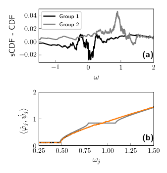
Figure 6: Numerical sampling leads to instabilities of the frequency distribution. This system uses the same parameters $\bar{\omega}_{2}=1$, $\gamma_{2}=0.2$ and a similar coupling of $K=0.48$ to Fig. 3(b) and Fig. 5 with $N_{1}=N_{2}=1000$. In (a), the difference between the sampled cumulative distribution function (sCDF) of $\omega_{1}$ and $\omega_{2}$ and the cumulative distribution function (CDF) of the corresponding Lorentz distribution in Eq. (2) is shown. In (b), the average frequencies are compared to the OA solution (gray line). Group 1 is shown as black circles, and group 2 as orange dots.

The Bellerophon state can be observed numerically for moderately big systems of the size of, e.g., 800 or 1000 oscillators. Their mean-field dynamics and their average frequencies fit very well to the predictions of the OA theory. In a few cases, a significant difference can be observed for non-entrained mean-fields. One such case is shown in Fig. 6. While the initial phase distribution is of not much importance, the sampling of the frequencies is. In the shown case, the frequencies of group 2 were oversampled close to $\Omega_{3}$, and group 1 was undersampled in $\Omega_{1}$. This undersampling leads to a weaker order parameter $R_{1}$ , which disturbs the oscillators that would normally form the cluster $\Omega_{3}$ in Fig. 6(b). This, in turn, leads to a significantly weaker order parameter $R_{2}\approx 0.22$ compared to the OA solution with $R_{2}\approx 0.36$.

VII Conclusion

We have shown the three different partial synchronous states in a two-group Kuramoto model with attractive and repulsive interaction. For weak coupling, each group can be well described by a forced Kuramoto model with an equal frequency distribution. For the group with the narrower distribution, the forcing can be disregarded.

Shortly after the coupling strength exceeds both groups critical coupling strength, there exists a Bellerophon state with multiple, step-like clusters of averagely entrained oscillators. The oscillators’ instantaneous dynamics in each cluster differ. This state leads to a non-entrainment of both groups mean-field frequencies. Still, they can be described by a similar Kuramoto model.

A further increase in the coupling strength leads to an entrainment, and the Bellerophon state shrinks and asymptotically approaches a one cluster state, as in the Kuramoto model. At this point, both groups synchronize stronger, and each approaches a Kuramoto model with a frequency distribution half as wide as the groups own.

The Bellerophon state is also reproduced numerically for moderately big systems of about 1000 oscillators. In special cases of sampling errors in the frequency distribution, the higher clusters are perturbed. As a result, the order parameter of group 2 becomes small compared to the analytical solution. So special care has to be taken when realizing such a configuration.

Open problems are the calculation of the critical coupling for the increase in synchronization and the order parameter of the second group in the Bellerophon state, as it differs quite a bit from the Kuramoto model solution.

Data Availability

The data that support the findings of this study are available from the corresponding author upon reasonable request.