Self-Attention Networks Can Process Bounded Hierarchical Languages

Abstract

Despite their impressive performance in NLP, self-attention networks were recently proved to be limited for processing formal languages with hierarchical structure, such as $\mathsf{Dyck}_{k}$, the language consisting of well-nested parentheses of $k$ types. This suggested that natural language can be approximated well with models that are too weak for formal languages, or that the role of hierarchy and recursion in natural language might be limited. We qualify this implication by proving that self-attention networks can process $\mathsf{Dyck}_{k,D}$, the subset of $\mathsf{Dyck}_{k}$ with depth bounded by $D$, which arguably better captures the bounded hierarchical structure of natural language. Specifically, we construct a hard-attention network with $D+1$ layers and $O(\log k)$ memory size (per token per layer) that recognizes $\mathsf{Dyck}_{k,D}$, and a soft-attention network with two layers and $O(\log k)$ memory size that generates $\mathsf{Dyck}_{k,D}$. Experiments show that self-attention networks trained on $\mathsf{Dyck}_{k,D}$ generalize to longer inputs with near-perfect accuracy, and also verify the theoretical memory advantage of self-attention networks over recurrent networks.

1 Introduction

Transformers Vaswani et al. (2017) are now the undisputed champions across several benchmark leaderboards in NLP. The major innovation of this architecture, self-attention, processes input tokens in a distributed way, enabling efficient parallel computation as well as long-range dependency modelling. The empirical success of self-attention in NLP has led to a growing interest in studying its properties, with an eye towards a better understanding of the nature and characteristics of natural language Tran et al. (2018); Papadimitriou and Jurafsky (2020).

In particular, it was recently shown that self-attention networks cannot process various kinds of formal languages Hahn (2020); Bhattamishra et al. (2020a), among which particularly notable is $\mathsf{Dyck}_{k}$, the language of well-balanced brackets of $k$ types. By the Chomsky-Schützenberger Theorem Chomsky and Schützenberger (1959), any context-free language can be obtained from a $\mathsf{Dyck}_{k}$ language through intersections with regular languages and homomorphisms. In other words, this simple language contains the essence of all context-free languages, i.e. hierarchical structure, center embedding, and recursion – features which have been long claimed to be at the foundation of human language syntax Chomsky (1956).

Consider for example the long-range and nested dependencies in English subject-verb agreement:

[hide label, edge unit distance=.4ex] [column sep=0.05cm] (Laws & (the lawmaker) & [writes] & [and revises])& [pass].

15. 23. 24.

The sentence structure is captured by $\mathsf{Dyck}_{2}$ string (()[][])[]. Given the state-of-the-art performance of Transformers in parsing natural language Zhang et al. (2020); He and Choi (2019), the $\mathsf{Dyck}_{k}$ blind spot seems very suggestive. If the world’s best NLP models cannot deal with this simple language — generated by a grammar with $k+2$ rules and recognized by a single-state pushdown automaton — does this not mean that the role of hierarchy and recursion in natural language must be limited? This question has of course, been extensively debated by linguists on the basis of both theoretical and psycholinguistic evidence Hauser et al. (2002); Frank et al. (2012); Nelson et al. (2017); Brennan and Hale (2019); Frank and Christiansen (2018).

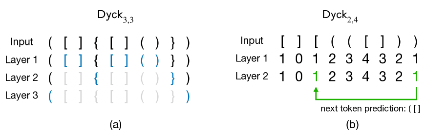
Figure 1: Illustrations of our self-attention network constructions to recognize and generate $\mathsf{Dyck}_{k,D}$. In construction (a), at each layer, the innermost brackets attend to their matching brackets and “cancel” each other, yielding “shallower” spans for successive layers to process. In construction (b), the first layer computes the depth of each token by attending to all previous tokens, while the second layer uses depth information to find the most recent unclosed open bractket in the history.

So, what can self-attention networks tell us about natural language and recursion? Here we provide a new twist to this question by considering $\mathsf{Dyck}_{k,D}$, the subset of $\mathsf{Dyck}_{k}$ with nesting depth at most $D$, and show that Transformers can process it. $\mathsf{Dyck}_{k,D}$ models bounded (or finite) recursion, thus captures the hierarchical structure of human language much more realistically. For example, center-embedding depth of natural language sentences is known to rarely exceed three Karlsson (2007); Jin et al. (2018), and while pragmatics, discourse, and narrative can result in deeper recursion in language Levinson (2014), there is arguably a relatively small limit to the depth as well.

In particular, we prove that self-attention networks can both recognize and generate $\mathsf{Dyck}_{k,D}$, with two conceptually simple yet different constructions (Figure 1). The first network requires $D+1$ layers and a memory size of $O(\log k)$ (per layer per token) to recognize $\mathsf{Dyck}_{k,D}$, using a distributed mechanism of parenthesis matching. The second network has two layers and memory size $O(\log k)$. It works by attending to all previous tokens to count the depth for each token in the first layer, and then uses this depth information to attend to the most recent unclosed open bracket in the second layer. Our constructions help reconcile the result in Hahn (2020) with the success of Transformers in handling natural languages.

Our proof requires certain assumptions about the positional encodings, an issue that is often considered in empirical papers Ke et al. (2021); Shaw et al. (2018); Wang et al. (2020); Shiv and Quirk (2019) but not in the more theoretical literature. First, positional encodings must have $\log n$ bits when the input length is $n$, as otherwise different positions would share the same representation. More importantly, positional encodings should support easy position comparisons, since token order is vital in formal language processing. Our experiments show that two standard practices, namely learnable or fixed sine/cosine positional encodings, cannot generalize well on $\mathsf{Dyck}_{k,D}$ beyond the training input lengths. In contrast, using a single fixed scalar monotonic positional encoding such as $\rm{pos}/n$ achieves near-perfect accuracy even on inputs significantly longer than the training ones. Our findings provide a novel perspective on the function of positional encodings, and implies that different applications of self-attention networks (in this case, natural vs. formal language) may require different model choices.

Our theoretical results also bring about interesting comparisons to recurrent networks (e.g. RNNs, LSTMs) in terms of the resource need to process hierarchical structure. While recurrent networks with finite precision need at least $\Omega(D\log k)$ memory to process $\mathsf{Dyck}_{k,D}$ Hewitt et al. (2020), our second construction requires only $O(\log k)$ memory but a $O(\log n)$ precision. In experiments where precision is not an issue for practical input lengths ($<10^{4}$), we confirm that a Transformer requires less memory than a LSTM to reach high test accuracies. This may help explain why Transformers outperform RNNs/LSTMs in syntactical tasks in NLP, and shed light into fundamental differences between recurrent and non-recurrent sequence processing.

2 Related work

Our work primarily relates to the ongoing effort of characterizing theoretical abilities Pérez et al. (2019); Bhattamishra et al. (2020b); Yun et al. (2020) and limitations of self-attention networks, particularly through formal hierarchical structures like $\mathsf{Dyck}_{k}$. Hahn (2020) proves that (even with positional encodings) hard-attention Transformers cannot model $\mathsf{Dyck}_{k}$, and soft-attention Transformers with bounded Lipschitz continuity cannot model $\mathsf{Dyck}_{k}$ with perfect cross entropy. Bhattamishra et al. (2020a) prove a soft-attention network with positional masking (but no positional encodings) can solve $\mathsf{Dyck}_{1}$ but not $\mathsf{Dyck}_{2}$. Despite the expressivity issues theoretically posed by the above work, empirical findings have shown Transformers can learn $\mathsf{Dyck}_{k}$ from finite samples and outperform LSTM Ebrahimi et al. (2020). Our work addresses the theory-practice discrepancy by using positional encodings and modeling $\mathsf{Dyck}_{k,D}$.

A parallel line of work with much lengthier tradition Elman (1990); Das et al. (1992); Steijvers and Grünwald (1996) investigates the abilities and limitations of recurrent networks to process hierarchical structures. In particular, RNNs or LSTMs are proved capable of solving context-free languages like $\mathsf{Dyck}_{k}$ given infinite precision Korsky and Berwick (2019) or external memory Suzgun et al. (2019); Merrill et al. (2020). However, Merrill et al. (2020) also prove RNNs/LSTMs cannot process $\mathsf{Dyck}_{k}$ without such assumptions, which aligns with experimental findings that recurrent networks perform or generalize poorly on $\mathsf{Dyck}_{k}$ Bernardy (2018); Sennhauser and Berwick (2018); Yu et al. (2019). Hewitt et al. (2020) propose to consider $\mathsf{Dyck}_{k,D}$ as it better captures natural language, and show finite-precision RNNs can solve $\mathsf{Dyck}_{k,D}$ with $\Theta(D\log k)$ memory.

For the broader NLP community, our results also contribute to settling whether self-attention networks are restricted to model hierarchical structures due to non-recurrence, a concern Tran et al. (2018) often turned into proposals to equip Transformers with recurrence Dehghani et al. (2019); Shen et al. (2018); Chen et al. (2018); Hao et al. (2019). On one hand, Transformers are shown to encode syntactic Lin et al. (2019); Tenney et al. (2019); Manning et al. (2020) and word order Yang et al. (2019) information, and dominate syntactical tasks in NLP such as constituency Zhang et al. (2020) and dependency He and Choi (2019) parsing. On the other hand, on several linguistically-motivated tasks like English subject-verb agreement Tran et al. (2018), recurrent models are reported to outperform Transformers. Our results help address the issue by confirming that distributed and recurrent sequence processing can both model hierarchical structure, albeit with different mechanisms and tradeoffs.

3 Preliminaries

3.1 Dyck Languages

Consider the vocabulary of $k$ types of open and close brackets $\Sigma=\cup_{i\in[k]}\{{\color[rgb]{0,0,1}{\langle}}_{i},{\color[rgb]{0,0,1}{\rangle}}_{i}\}$, and define $\text{Dyck}_{k}\subset\gamma\Sigma^{*}\omega$ ($\gamma,\omega$ being special start and end tokens) to be the formal language of well-nested brackets of $k$ types. It is generated starting from $\gamma X\omega$ through the following context-free grammar:

$$X\to\epsilon\ |\ {\color[rgb]{0,0,1}{\langle}}_{i}\ X\ {\color[rgb]{0,0,1}{\rangle}}_{i}\ X\quad(i\in[k])$$ (1)

where $\epsilon$ denotes the empty string.

Intuitively, $\mathsf{Dyck}_{k}$ can be recognized by sequential scanning with a stack (i.e., a pushdown automaton). Open brackets are pushed into the stack, while a close bracket causes the stack to pop, and the popped open bracket is compared with the current close bracket (they should be of the same type). The depth of a string $w_{1:n}$ at position $i$ is the stack size after scanning $w_{1:i}$, that is, the number of open brackets left in the stack:

$$d(w_{1:i})=\mathsf{count}(w_{1:i},{\color[rgb]{0,0,1}{\langle}})-\mathsf{count}(w_{1:i},{\color[rgb]{0,0,1}{\rangle}})$$ (2)

Finally, we define $\mathsf{Dyck}_{k,D}$ to be the subset of $\mathsf{Dyck}_{k}$ strings with depth bounded by $D$:

$$\mathsf{Dyck}_{k,D}=\left\{w_{1:n}\in\text{Dyck}_{k}\left|\\ \max_{i\in[n]}d(w_{1:i})\leq D\right.\right\}$$

That is, a string in $\mathsf{Dyck}_{k,D}$ only requires a stack with bounded size $D$ to process.

3.2 Self-attention Networks

We consider the encoder part of the original Transformer Vaswani et al. (2017), which has multiple layers of two blocks each: (i) a self-attention block and (ii) a feed-forward network (FFN). For an input string $w_{1:n}\in\Sigma^{*}$, each input token $w_{i}$ is converted into a token embedding via $f_{e}:\Sigma\to\mathbb{R}^{d_{\operatorname{model}}}$, then added with a position encoding $\mathbf{p}_{i}\in\mathbb{R}^{d_{\operatorname{model}}}$. Let $\mathbf{x}_{i,\ell}\in\mathbb{R}^{d_{\operatorname{model}}}$ be the $i$-th representation of the $\ell$-th layer ($i\in[n],\ell\in[L]$). Then

$$\mathbf{x}_{i,0} =f_{e}(w_{i})+\mathbf{p}_{i}$$ (3)

$$\mathbf{a}_{i,\ell} =\operatorname{Att}_{\ell}(Q_{\ell}(\mathbf{x}_{i}),K_{\ell}(\mathbf{x}),V_{\ell}(\mathbf{x}))$$ (4)

$$\mathbf{x}_{i,\ell+1} =F_{\ell}(\mathbf{a}_{i,\ell})$$ (5)

Attention

In each head of a self-attention block, the input vectors $\mathbf{x}_{1:n}$ undergo linear transforms $Q,K,V$ yielding query, key, and value vectors. They are taken as input to a self-attention module, whose $t$-th output, $\operatorname{Att}(Q\mathbf{x}_{i},K\mathbf{x},V\mathbf{x})$, is a vector $\mathbf{a}_{i}=\sum_{j\in[T]}\alpha_{j}V\mathbf{x}_{j}$, where $\alpha_{1:n}=\text{softmax}(\langle Q\mathbf{x}_{i},K\mathbf{x}_{1}\rangle,\cdots,\langle Q\mathbf{x}_{i},K\mathbf{x}_{n}\rangle)$. The final attention output is the concatenation of multi-head attention outputs. We also consider variants of the basic model along these directions:

(i) Hard attention, as opposed to soft attention described above, where hardmax is used in place for softmax (i.e.  $\operatorname{Att}(Q\mathbf{x}_{i},K\mathbf{x},V\mathbf{x})=V\mathbf{x}_{j^{\prime}}$ where $j^{\prime}=\arg\max_{j}\langle Q\mathbf{x}_{i},K\mathbf{x}_{j}\rangle$). Though impractical for NLP, it has been used to model formal languages Hahn (2020).

(ii) Positional masking, where $\alpha_{1:i}$ (past) or $\alpha_{i:n}$ (future) is masked for position $i$. Future-positional masking is usually used to train auto-regressive models like GPT-2 Radford et al. (2019).

Feed-forward network

A feed-forward network $F$ transforms each self-attention output vector $\mathbf{a}_{i}\to F(\mathbf{a}_{i})$ individually. It is usually implemented as a multi-layer perceptron (MLP) with ReLU activations. Residual connections He et al. (2016) and layer normalization Ba et al. (2016) are two optional components to aid learning.

Positional encodings

Vaswani et al. (2017) proposes two kinds of positional encoding: (i) Fourier features Rahimi and Recht (2007), i.e. sine/cosine values of different frequencies; (ii) learnable features for each position. In this work we propose to use a single scalar $i/n$ to encode position $i\in[n]$, and show that it helps process formal languages like $\mathsf{Dyck}_{k,D}$, both theoretically and empirically.

Precision and memory size

We define precision to be the number of binary bits used to represent each scalar, and memory size per layer ($d_{\operatorname{model}}$) to be the number of scalars used to represent each token at each layer. The memory size ($L\cdot d_{\operatorname{model}}$) is the total memory used for each token.

3.3 Language Generation and Recognition

For a Transformer with $L$ layers and input $w_{1:i}$, we can use a decoder (MLP + softmax) on the final token output $\mathbf{x}_{i,L}$ to predict $w_{i+1}$. This defines a language model $f_{\theta}(w_{i+1}|w_{i})$ where $\theta$ denotes Transformer and decoder parameters. We follow previous work Hewitt et al. (2020) to define how a language model can generate a formal language:

Definition 3.1 (Language generation).

Language model $f_{\theta}$ over $\Sigma^{\star}$ generates a language $\mathcal{L}\subseteq\Sigma^{\star}$ if there exists $\epsilon>0$ such that $\mathcal{L}=\{w_{1:n}\in\Sigma^{\star}\ |\ \forall i\in[n],f_{\theta}(w_{i}|w_{1:i-1})\geq\epsilon\}$.

We also consider language recognition by a language classifier $g_{\theta}(w_{1:i})$, where a decoder on $\mathbf{x}_{i,L}$ instead predicts a binary label.

Definition 3.2 (Language recognition).

Language classifier $g_{\theta}$ over $\Sigma^{\star}$ recognizes a language $\mathcal{L}\subseteq\Sigma^{\star}$ if $\mathcal{L}=\{w_{1:n}\in\Sigma^{\star}\ |g_{\theta}(w_{1:n})=1\}$.

4 Theoretical Results

In this section we state our theoretical results along with some remarks. Proof sketches are provided in the next section, and details in Appendix A,B,C.

Theorem 4.1 (Hard-attention, $\mathsf{Dyck}_{k,D}$ recognition).

For all $k,D\in\mathbb{N}^{+}$, there exists a $(D+1)$-layer hard-attention network that can recognize $\mathsf{Dyck}_{k,D}$. It uses both future and past positional masking heads, positional encoding of the form $i/n$ for position $i$, $O(\log k)$ memory size per layer, and $O(\log n)$ precision, where $n$ is the input length.

Theorem 4.2 (Soft-attention, $\mathsf{Dyck}_{k,D}$ generation).

For all $k,D\in\mathbb{N}^{+}$, there exists a 2-layer soft-attention network that can generate $\mathsf{Dyck}_{k,D}$. It uses future positional masking, positional encoding of form $i/n$ for position $i$, $O(\log k)$ memory size per layer, and $O(\log n)$ precision, where $n$ is the input length. The feed-forward networks use residual connection and layer normalization.

Theorem 4.3 (Precision lower bound).

For all $k\in\mathbb{N}^{+}$, no hard-attention network with $o(\log n)$ precision can recognize $\mathsf{Dyck}_{k,2}$ where $n$ is the input length.

Required precision

Both constructions require a precision increasing with input length, as indicated by Theorem 4.3. The proof of the lower bound is inspired by the proof in Hahn (2020), but several technical improvements are necessary; see Appendix C. Intuitively, a vector with a fixed dimension and $o(\log n)$ precision cannot even represent $n$ positions uniquely. The required precision is not unreasonable, since $\log n$ is a small overhead to the $n$ tokens the system has to store.

Comparison to recurrent processing

Hewitt et al. (2020) constructs a 1-layer RNN to generate $\mathsf{Dyck}_{k,D}$ with $\Theta(D\log k)$ memory, and proves it is optimal for any recurrent network. Thus Theorem 4.2 establishes a memory advantage of self-attention networks over recurrent ones. However, this is based on two tradeoffs: (i) Precision. Hewitt et al. (2020) assumes $O(1)$ precision while we require $O(\log n)$. (ii) Runtime. Runtime of recurrent and self-attention networks usually scale linearly and quadratically in $n$, respectively.

Comparison between two constructions

Theorem 4.2 requires fewer layers ($2$ vs. $D$) and memory size ($O(\log k)$ vs. $O(D\log k)$) than Theorem 4.1, thanks to the use of soft-attention, residual connection and layer normalization. Though the two constructions are more suited to the tasks of recognition and generation respectively (Section 5), each of them can also be modified for the other task.

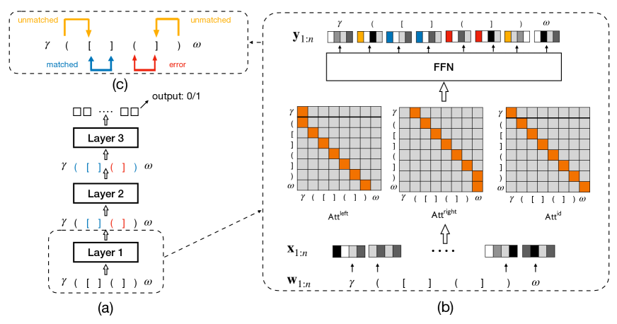
Figure 2: Our construction for Theorem 4.1. (a) The network has multiple identical layers to match brackets and detect errors. (b) Each layer consists of three hard-attention heads so that a token attends to itself and the nearest unmatched tokens on both sides, and uses representations from these positions to update its state. (c) Each position can be in three states: matched, error, or unmatched.

Connection to $\mathsf{Dyck}_{k}$

In Hahn (2020) it is shown that no hard-attention network can recognize $\mathsf{Dyck}_{k}$ even for $k=1$. Theorem 4.1 establishes that this impossibility can be circumvented by bounding the depth of the Dyck language. Hahn (2020) also points out soft-attention networks can be limited due to bounded Lipschitz continuity. In fact, our Theorem 4.2 construction can also work on $\mathsf{Dyck}_{k}$ with some additional assumptions (e.g. feed $n$ also in input embeddings), and we circumvent the impossibility by using laying normalization, which may have an $O(n)$ Lipschitz constant. More details are in Appendix B.4.

5 Constructions

5.1 $(D+1)$-layer Hard-Attention Network

Our insight underlying the construction in Theorem 4.1 is that, by recursively removing matched brackets from innermost positions to outside, each token only needs to attend to nearest unmatched brackets to find its matching bracket or detect error within $D$ layers. Specifically, at each layer $\ell\leq D$, each token will be in one of three states (Figure 2 (c)): (i) Matched, (ii) Error, (iii) Unmatched, and we leverage hard-attention to implement a dynamic state updating process to recognize $\mathsf{Dyck}_{k,D}$.

Representation

For an input $w_{1:n}\in\gamma\Sigma^{*}\omega$, the representation at position $i$ of layer $\ell$ has five parts $\mathbf{x}_{i,\ell}=[\mathbf{t}_{i},o_{i},p_{i},m_{i,\ell},e_{i,\ell}]$: (i) a bracket type embedding $\mathbf{t}_{i}\in\mathbb{R}^{\lceil\log k\rceil}$ that denotes which bracket type ($1\cdots k$) the token is (or if the token is start/end token); (ii) a bracket openness bit $o_{i}\in\{0,1\}$, where $1$ denotes open brackets (or start token) and $0$ denotes close one (or end token); (iii) a positional encoding scalar $p_{i}=i/n$; (iv) a match bit $m_{i,\ell}\in\{0,1\}$, where $1$ denotes matched and $0$ unmatched; (v) an error bit $e_{i,\ell}\in\{0,1\}$, where $1$ denotes error and $0$ no error. Token identity parts $\mathbf{t}_{i},o_{i},p_{i}$ are maintained unchanged throughout layers. The match and error bits are initialized as $e_{i,0}=m_{i,0}=0$.

The first $D$ layers have identical self-attention blocks and feed-forward networks, detailed below.

Attention

Consider the $\ell$-th self-attention layer ($\ell\in[D]$), and denote $\mathbf{x}_{i}=\mathbf{x}_{i,\ell-1}$, $m_{i}=m_{i,\ell-1}$, $\mathbf{a}_{i}=\mathbf{a}_{i,\ell}$, $\mathbf{y}_{i}=\mathbf{x}_{i,\ell}$ for short. We have 3 attention heads: (i) an identity head $\operatorname{Att}^{\mathsf{id}}$, where each token only attends to itself with attention output $\mathbf{a}^{\operatorname{id}}_{i}=\mathbf{x}_{i}$; (ii) a left head $\operatorname{Att}^{\mathsf{left}}$ with future positional masking; (iii) a right head $\operatorname{Att}^{\mathsf{right}}$ with past positional masking. The query, key, and value vectors for $\operatorname{Att}^{\mathsf{left}}$ are defined as $Q\mathbf{x}_{i}=1\in\mathbb{R}$, $K\mathbf{x}_{i}=p_{i}-m_{i}\in\mathbb{R}$, $V\mathbf{x}_{i}=\mathbf{x}_{i}\in\mathbb{R}^{d_{\operatorname{model}}}$, so that

$$\mathbf{a}^{\mathsf{left}}_{i}=\mathbf{x}_{j_{1}},\quad j_{1}=\arg\max_{j<i}(j/n-m_{j})$$

is the representation of the nearest unmatched token to $i$ on its left side. Similarly

$$\mathbf{a}^{\mathsf{right}}_{i}=\mathbf{x}_{j_{2}},\quad j_{2}=\arg\max_{j>i}(1-j/n-m_{j})$$

is the representation of the nearest unmatched token to $i$ on its right side. The attention output for position $i$ is the concatenation of these three outputs: $\mathbf{a}_{i}=[\mathbf{a}_{i}^{\mathsf{id}},\mathbf{a}_{i}^{\mathsf{left}},\mathbf{a}_{i}^{\mathsf{right}}]=[\mathbf{x}_{i},\mathbf{x}_{j_{1}},\mathbf{x}_{j_{2}}]$.

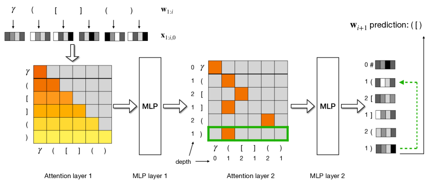
Figure 3: Our construction for Theorem 4.2. The first self-attention layer calculates token depths, while the second layer uses them so that each token attends to the closest unmatched open bracket ign the history, which is useful for next token prediction.

Feed-forward network (FFN)

Following the notation above, the feed-forward network $F:\mathbf{a}_{i}\to\mathbf{y}_{i}$ serves to update each position’s state using information from $\mathbf{x}_{j_{1}},\mathbf{x}_{j_{2}}$. The high level logic (Figure 2 (c)) is that, if $w_{i}$ is an open bracket, its potential matching half should be $w_{j}=w_{j_{2}}$ ($j_{2}>i$), otherwise it should be $w_{j}=w_{j_{1}}$ ($j_{1}<i$). If $w_{i}$ and $w_{j}$ are one open and one close, they either match (same type) or cause error (different types). If $w_{i}$ and $w_{j}$ are both open or both close, no state update is done for position $i$. Besides, token identity parts $\mathbf{t}_{i},o_{i},p_{i}$ are copied from $\mathbf{a}^{\mathsf{id}}_{i}$ to pass on. The idea can be translated into a language of logical operations ($\wedge,\vee,\neg$) plus a $\textsc{same}(\mathbf{t},\mathbf{t}^{\prime})$ operation, which returns $1$ if vectors $\mathbf{t}=\mathbf{t}^{\prime}$ and $0$ otherwise:

$$\mathbf{y}_{i} =[\mathbf{t}_{i},o_{i},p_{i},m^{\prime}_{i},e^{\prime}_{i}]$$

$$m^{\prime}_{i} =m_{i}\vee(o_{i}\wedge\neg o_{j_{2}}\wedge s_{2})\vee(\neg o_{i}\wedge o_{j_{1}}\wedge s_{1})$$

$$e^{\prime}_{i} =e_{i}\vee(o_{i}\wedge\neg o_{j_{2}}\wedge\neg s_{2})\vee(\neg o_{i}\wedge o_{j_{1}}\wedge\neg s_{1})$$

$$s_{1} =\textsc{same}(\mathbf{t}_{i},\mathbf{t}_{j_{1}})\quad s_{2}=\textsc{same}(\mathbf{t}_{i},\mathbf{t}_{j_{2}})$$

As we show in Appendix A, a multi-layer perception with ReLU activations can simulate all operations $(\wedge,\vee,\neg,\textsc{same})$, thus the existence of our desired FFN.

Final layer

At the $(D+1)$-th layer, the self attention is designed as $Q\mathbf{x}_{i}=1\in\mathbb{R}$, $K\mathbf{x}_{i}=e_{i}+1-m_{i}\in\mathbb{R}$, $V\mathbf{x}_{i}=(e_{i},m_{i})\in\mathbb{R}^{2}$. If all brackets are matched without error ($(e_{i},m_{i})=(0,1)$), all keys would be $0$, and the attention output of the last token $\mathbf{a}_{n}$ would be $(0,1)$. If any bracket finds error $(e_{i}=1)$ or is not matched $(m_{i}=0)$, the key would be at least $1$ and $\mathbf{a}_{n}$ would not be $(0,1)$. An FNN that emulates $(a,b)\mapsto\neg a\wedge b$ will deliver $y_{n}$ as the recognition answer.

5.2 Two-layer Soft-Attention Network

Our Theorem 4.2 construction takes advantage of soft attention, residual connection, and layer normalization to calculate each token depth and translate it into a vector form at the first layer. Using the depth information, at the second layer each $w_{i}$ can attend to the stack-top open bracket at the position, in order to decide if open brackets or which type of close brackets can be generated as the next token (Figure 3).

Representation

The representation at position $i$, layer $\ell$ has four parts $\mathbf{x}_{i,\ell}=[\mathbf{t}_{i},o_{i},p_{i},\mathbf{d}_{i,\ell}]$, with bracket type embedding $\mathbf{t}_{i}$, bracket openness bit $o_{i}$, position encoding $p_{i}$ already specified in Section 5.1. The last part $\mathbf{d}_{i,\ell}\in\mathbb{R}^{2}$ is used to store depth information for position $i$, and initialized as $\mathbf{d}_{i,0}=(0,0)$.

First Layer – Depth Counting

The first self-attention layer has two heads, where an $\operatorname{Att}^{\operatorname{id}}$ head is still used to inherit $\mathbf{t}_{i},o_{i},\mathbf{p}_{i}$, and a future positional masking head $\operatorname{Att}^{\mathsf{d}}$ aims to count depth with $Q\mathbf{x}_{i}=K\mathbf{x}_{i}=1$ and $V\mathbf{x}_{i}=2o_{i}-1$, resulting in uniform attention scores and attention output $a^{d}_{i}=\sum_{j\leq i}\frac{1}{i}\cdot(2o_{j}-1)=d(w_{1:i})/i$.

However, our goal is to enable matching based on depth $d_{i}=d(w_{1:i})$, and the attention output $d_{i}/i$ isn’t readily usable for such a purpose: the denominator $i$ is undesirable, and even a scalar $d_{i}$ cannot easily attend to the same value using dot-product attention. Thus in the first feed-forward network, we leverage residual connection and layer normalization to transform

$$d_{i}/i \mapsto\mathbf{d}_{i}=(\cos(\theta(d_{i})),\sin(\theta(d_{i})))$$ (6)

where $\theta(d)=\arctan\left(\frac{d}{D+2-d}\right)$ has an unique value for every $d\in\{0,\cdots,D+1\}$, so that

$$\mathbf{d}_{i}\cdot\mathbf{d}_{j}\begin{cases}=1&d_{i}=d_{j}\\ <1-\frac{1}{10D^{2}}&d_{i}\neq d_{j}\end{cases}$$ (7)

The representation by the end of first layer is $\mathbf{x}_{i,1}=[\mathbf{t}_{i},o_{i},p_{i},\mathbf{d}_{i}]$. The full detail for the first FFN is in Appendix B.1.

Second layer – Depth Matching

The second self-attention layer has a depth matching hard-attention head $\operatorname{Att}^{\mathsf{match}}$, with query, key, value vectors as $Q\mathbf{x}_{i}=[20D^{2}\cdot\mathbf{d}_{i},1,2]\in\mathbb{R}^{4}$, $K\mathbf{x}_{i}=[\mathbf{d}_{i},p_{i},o_{i}]\in\mathbb{R}^{4}$, $V\mathbf{x}_{i}=\mathbf{x}_{i}$, so that attention score

$$\langle Q\mathbf{x}_{i},K\mathbf{x}_{j} \rangle=20D^{2}\mathbf{d}_{i}\cdot\mathbf{d}_{j}+j/n+2o_{j}$$

$$\begin{cases}=20D^{2}+2+j/n&d_{i}=d_{j},o_{j}=1\\ \leq 20D^{2}+1&\text{otherwise}\end{cases}$$

would achieve its maximum when $w_{j}$ ($j\leq i$) is the open bracket (or start token) closest to $w_{i}$ with $d_{j}=d_{i}$. The attention output is $\mathbf{a}_{i}=[\mathbf{a}^{\operatorname{id}}_{i},\mathbf{a}^{\mathsf{match}}_{i}]=[\mathbf{x}_{i},\mathbf{x}_{j}]$ where $j=\max\{j\leq i|d_{i}=d_{j}\wedge o_{j}=1\}$.

With such a $[\mathbf{x}_{i},\mathbf{x}_{j}]$, the second-layer FFN can readily predict what $w_{i+1}$ could be. It could be any open bracket when $d_{i}<D$ (i.e. $\cos(\theta(d_{i}))>\cos(\theta(D))$), and it could be a close bracket with type as $\mathbf{t}_{j}$ (or end token if $w_{j}$ is start token). The detailed construction for such a FFN is in Appendix B.2.

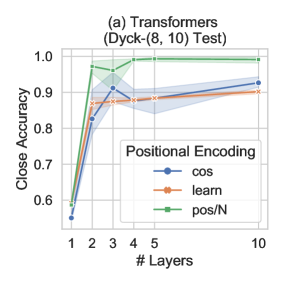
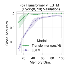
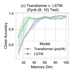
Figure 4: Results on $\mathsf{Dyck}_{8,10}$ validation set (same input lengths as training) and test set (longer inputs). (a) compares Transformers of different layers ($L\in\{1,2,3,4,5,10\}$) and with different positional encodings (cos, learn,pos/N) on the test set. (b) and (c) compare a 2-layer Transformer (pos/N) with a 1-layer LSTM over varying memory sizes on the validation and test sets respectively.

On $\mathsf{Dyck}_{k}$ Generation

In fact, this theoretical construction can also generate $\mathsf{Dyck}_{k}$, as intuitively the $O(\log n)$ precision assumption allows counting depth up to $O(n)$. But it involves extra conditions like feeding $n$ into network input, and may not be effectively learned in practice. Please refer to details in Appendix B.4.

Connection to Empirical Findings

Our theoretical construction explains the observation in Ebrahimi et al. (2020): the second layer of a two-layer Transformer trained on $\mathsf{Dyck}_{k}$ often produces virtually hard attention, where tokens attend to the stack-top open bracket (or start token). It also explains why such a pattern is found less systematically as input depth increases, as (6) is hard to learn and generalize to unbounded depth in practice.

6 Experiments

Our constructions show the existence of self-attention networks that are capable of recognizing and generating $\mathsf{Dyck}_{k,D}$. Now we bridge theoretical insights into experiments, and study whether such networks can be learned from finite samples and generalize to longer input. The answer is affirmative when the right positional encodings and memory size are chosen according to our theory.

We first present results on $\mathsf{Dyck}_{8,10}$ (Section 6.1) as an example $\mathsf{Dyck}_{k,D}$ language to investigate the effect of different positional encoding schemes, number of layers, and hidden size on the Transformer performance, and to compare with the LSTM performance. We then extend the Transformer vs. LSTM comparison on more $\mathsf{Dyck}_{k,D}$ languages ($k\in\{2,8,32,128\}$, $D\in\{3,5,10,15\}$) in Section 6.2. Finally, we apply the novel scalar positional encoding to natural language modeling with some preliminary findings (Section 6.3).

6.1 Evaluation on $\mathsf{Dyck}_{8,10}$

Setup

For $\mathsf{Dyck}_{8,10}$, we generate training and validation sets with input length $n\leq 700$, and test set with length $700<n\leq 1400$. We train randomly initialized Transformers using the Huggingface library Wolf et al. (2019), with one future positional masking head, $L\in\{1,2,3,4,5,10\}$ layers, and a default memory size $d_{\operatorname{model}}=30$. We search for learning rates in $\{0.01,0.001\}$, run each model with 3 trials, and report the average accuracy of generating close brackets, the major challenge of $\mathsf{Dyck}_{k,D}$. More setup details are in Appendix D.1.

Positional Encodings

We compare 3 types of positional encodings: (i) Fourier features (cos); (ii) learnable features (learn); (iii) a scalar $i/6000$ for position $i$ (pos/N). Note that (i, ii) are original proposals in Vaswani et al. (2017), where positional encoding vectors are added to the token embeddings, while our proposal (iii) encodes the position as a fixed scalar separated from token embeddings.

On the validation set of $\mathsf{Dyck}_{8,10}$ (see Appendix D.2), all three models achieve near-perfect accuracy with $L\geq 2$ layers. On the test set (Figure 4(a)) however, only pos/N maintains near-perfect accuracy, even with $L=10$ layers. Meanwhile, learn and cos fail to generalize, because encodings for position $700<i\leq 1400$ are not learned (for learn) or experienced (for cos) during training. The result validates our theoretical construction, and points to the need for separate and systemic positional encodings for processing long and order-sensitive sequences like $\mathsf{Dyck}_{k,D}$.

Memory Size and Comparison with LSTM

We compare a two-layer Transformer (pos/N) with a one-layer LSTM Hochreiter and Schmidhuber (1997) using varying per-layer memory sizes $d_{\operatorname{model}}\in\{10,20,\cdots,100\}$. As Figure 4 (b) shows, the Transformer consistently outperforms the LSTM on the validation set. On the test set (Figure 4 (c)), the Transformer and the LSTM first achieve a $>90\%$ accuracy using $d_{\operatorname{model}}=20$ and $40$ respectively, and an accuracy of $>95\%$ with $d_{\operatorname{model}}=30$ and $50$, respectively. These findings agree with our theoretical characterization that self-attention networks have a memory advantage over recurrent ones.

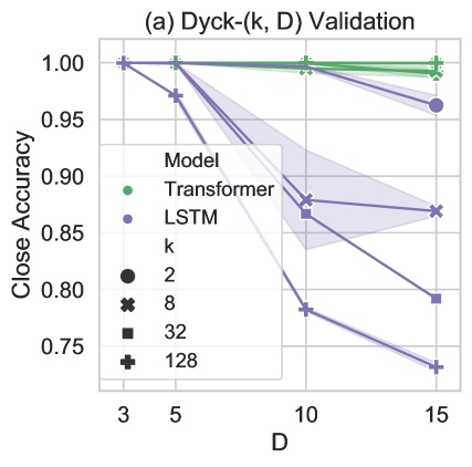
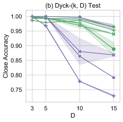
Figure 5: Results on more $\mathsf{Dyck}_{k,D}$ languages.

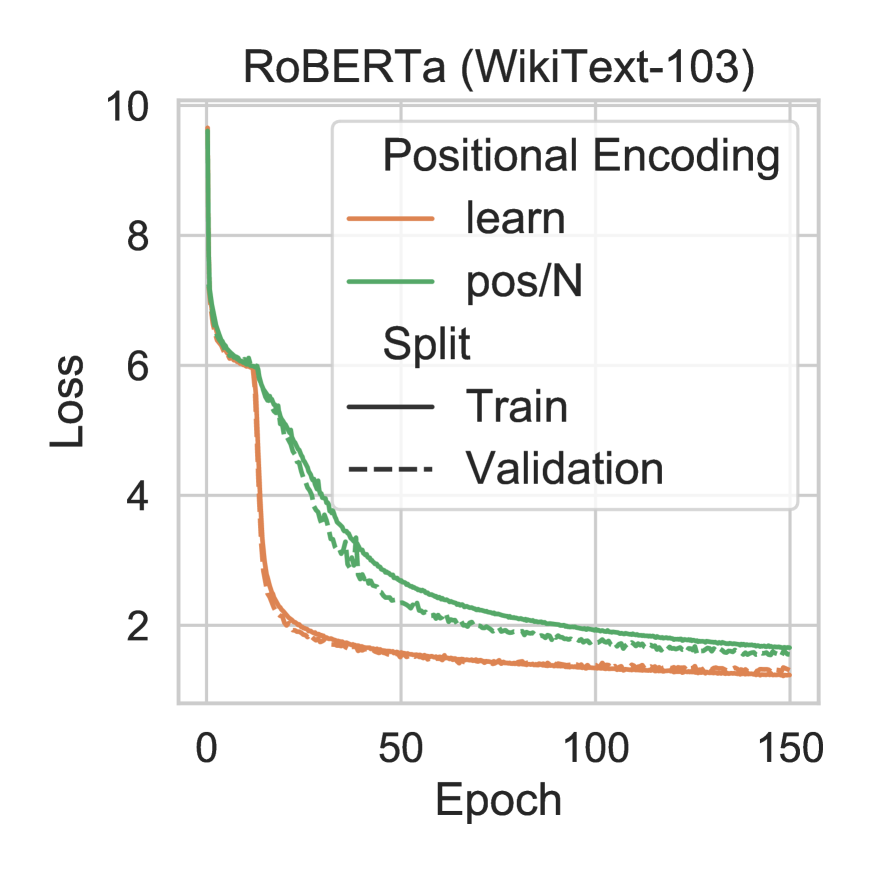
Figure 6: Results on WikiText-103.

6.2 Evaluation on More $\mathsf{Dyck}_{k,D}$ Languages

Setup

In order to generalize some of the above results, we generate a wide range of $\mathsf{Dyck}_{k,D}$ languages with different vocabulary sizes ($k\in\{2,8,32,128\}$) and recursion bounds ($D\in\{3,5,10,15\}$). We continue to compare the one-layer LSTM versus the two-layer Transformer (pos/N). For each model on each language, we perform a hyperparameter search for learning rate in {0.01, 0.001} and memory size $d_{\operatorname{model}}\in\{10,30,50\}$, and report results from the best setting based on two trials for each setting.

Results

The validation and test accuracy of the models are reported in Figure 6, and more fine-grained results for each $d_{\operatorname{model}}\in\{10,30,50\}$ are in Appendix D.2. The Transformer attains a $>99.9\%$ validation accuracy and a $>94\%$ test accuracy across all languages, strengthening the main claim that self-attention networks can learn $\mathsf{Dyck}_{k,D}$ languages and generalize to longer input. On the other hand, the validation and test accuracy of the LSTM model are less than $80\%$ when the vocabulary size and recursion depth are large, i.e. $(k,D)\in\{(32,15),(128,10),(128,15)\}$, which reconfirms Transformers’ memory advantage under limited memory ($d_{\operatorname{model}}\leq 50$).

6.3 Evaluation on WikiText-103

In Section 6.1, we show a Transformer with the scalar positional encoding scheme (pos/N) can learn $\mathsf{Dyck}_{k,D}$ and generalize to longer input, while traditional positional encoding schemes ((cos), (learn)) lead to degraded test performance. To investigate whether such a novel scheme is also useful in NLP tasks, we train two RoBERTa models (pos/N, learn) from scratch on the WikiText-103 dataset Merity et al. (2017) for 150 epochs.

Figure 6 shows the masked language modeling loss on both training and validation sets. By the end of the training, pos/N has a slightly larger validation loss (1.55) than learn (1.31). But throughout the optimization, pos/N shows a gradual decrease of loss while learn has a sudden drop of loss around 20-30 epochs. We believe it will be interesting for future work to explore how pos/N performs on different downstream tasks, and why pos/N seems slightly worse than learn (at least on this MLM task), though theoretically it provides the complete positional information for Transformers. These topics will contribute to a deeper understanding of positional encodings and how Transformers leverage positional information to succeed on different tasks.

7 Discussion

In this paper, we theoretically and experimentally demonstrate that self-attention networks can process bounded hierarchical languages $\mathsf{Dyck}_{k,D}$, even with a memory advantage over recurrent networks, despite performing distributed processing of sequences without explicit recursive elements. Our results may explain their widespread success at modeling long pieces of text with hierarchical structures and long-range, nested dependencies, including coreference, discourse and narratives. We hope these insights can enhance knowledge about the nature of recurrence and parallelism in sequence processing, and lead to better NLP models.

Ethical Consideration

Our work is mainly theoretical with no foreseeable ethical issues.

Appendix A Construction Details of Section 5.1

We provide missing details on the construction of $(D+1)$-layer Transformer with hard attention. In particular, we prove that neural networks are capable of simulating logic gates: and, or, not, same and arithmic gates: greaterthan and equal gate. For input $x,y\in\mathbb{R}$, the greaterthan satisfies that $\textsc{greaterthan}(x,y)=1$ if $x\geq y+c$ and $\textsc{greaterthan}(x,y)=0$ when $x<y$; the equal gate satisfies $\textsc{equal}(x,y)=1$ if $x=y$ and $\textsc{equal}(x,y)=0$ when $x<y-c$ or $x>y+c$. Here $c$ is a constant independent of $x,y$.

Lemma A.1.

A constant layer neural network can simulate logic gates: and, or, not, same and arithmic gates: greaterthan, equal.

Proof.

Our construction is as follows.

(1) and gate. Given input $x_{1},\ldots,x_{m}\in\{0,1\}$, we compute $z=\max\{x_{1}+\cdots+x_{m}-m+1,0\}.$ We conclude that $z=1$ iff $x_{1}=\cdots=x_{m}=1$ and $z=0$ otherwise.

(2) not gate. Given input $x\in\{0,1\}$, it suffices to compute $z=\max\{1-x,0\}$.

(3) or gate. Given input $x_{1},\ldots,x_{m}\in\{0,1\}$, we compute $z=\max\{1-\max\{1-x_{1}-\cdots-x_{m},0\},0\}.$ It is easy to see that $z=1$ iff one of $x_{i}=1$ ($i\in[m]$) and $z=0$ otherwise.

(3) same gate. Given input $x_{1},\ldots,x_{m}\in\{0,1\}$ and $y_{1},\ldots,y_{m}\in\{0,1\}$. The same gate is equivalent to $z=\left((x_{1}\vee\overline{y}_{1})\wedge(\overline{x}_{1}\vee y_{1})\right)\vee\cdots\vee\left((x_{m}\vee\overline{y}_{m})\wedge(\overline{x}_{m}\vee y_{m})\right)$. We can construct it using logic gates: and, or, not .

(4) greaterthan gate. Given $x,y\in\mathbb{R}$, compute $z_{1}=\frac{1}{c}\max\{c-\max\{x-y,0\},0\}$, we have that $z_{1}=0$ when $x>y+c$ and $z=1$ when $x\leq y$. Taking $z=\max\{1-z_{1},0\}$ completes the construction.

(5) equal gate. Given $x,y\in\mathbb{R}$. Let $z_{1}=\textsc{GreaterEqual}(x,y)$ and $z_{2}=\textsc{GreaterEqual}(y,x)$. It suffices to take $z=\neg z_{1}\wedge\neg z_{2}$.∎

We have proved a $(D+1)$-layer Transformer with hard attention can recognize $\mathsf{Dyck}_{k,D}$. We next extend the construction for recognition task to generation task and prove that a $D$ layer Transformer is capable of generating $\mathsf{Dyck}_{k,D}$.

Corollary A.2.

$\forall k,D\in\mathbb{N}^{+}$, there exists a $D$-layer hard-attention network that can generate $\mathsf{Dyck}_{k,D}$. It uses both a future-position masking head and a past-position masking head, a $O(\log k)$ memory size, and $O(\log n)$ precision for processing input length up to $n$.

Proof.

In the generation task, we are given an input segment $\mathbf{w}=\gamma w_{1}w_{2}\ldots w_{T}$ ($\gamma$ is the start token) and we want to generate the next symbol $w_{T+1}$. We augment the input with a generation token $\nu$ at the end and feed input $\gamma w_{1}w_{2}\ldots w_{T}\nu$ to the Transformer, The output probability distribution is contained in $\mathbf{y}_{T+2,\ell}$, i.e., the internal representation of the generation token $\nu$ at the last layer.

In the generation task, we add two extra parts for the representation at position $i$ of layer $\ell$ and augment the position encoding: $\mathbf{x}_{i,\ell}=[\mathbf{t}_{i},o_{i},\mathbf{p}_{i},m_{i,\ell},e_{i,\ell},\widetilde{\mathbf{m}}_{i,\ell},c_{i,\ell}]$. In particular, we add $\widetilde{\mathbf{m}}_{i,\ell}$ and $c_{i,\ell}$ to record the matched open bracket and the depth of generation token separately. The position encoding consists of three parts: $p_{i_{1}}=\frac{i}{n}$, $p_{i_{2}}=i$ and $p_{i_{3}}=n$, where $n$ denotes an upper bound on the length of sequence we aim to generate.

The first $D$ layers are the same as the recognition task, except that we also record the matched open bracket of the generation token and count its depth. For ease of presentation, we assume there is a special bit $g_{i}$ contained in $\mathbf{t}_{i}$ that indicates the generation token. We add the following operations to each FNN layer,

$$c_{i,\ell}= ~{}c_{i,\ell-1}+m^{\prime}_{i}$$

$$\widetilde{\mathbf{m}}_{i,\ell}= ~{}\widetilde{\mathbf{m}}_{i,\ell-1}\wedge\widetilde{\mathbf{m}}^{\prime}_{i}$$

where $m^{\prime}_{i}\in\{0,1\}$, $\widetilde{\mathbf{m}}^{\prime}_{i}\in\{0,1\}^{\lceil\log k\rceil}$ obeys

$$m^{\prime}_{i} =g_{i}\wedge((o_{i}\wedge\neg o_{j_{2}}\wedge s_{2})\vee(\neg o_{i}\wedge o_{j_{1}}\wedge s_{1}))$$

$$\widetilde{\mathbf{m}}^{\prime}_{i} =g_{i}\wedge\neg m_{i}\wedge o_{j_{1}}\wedge\mathbf{t}_{j_{1}}$$

$$s_{1} =\textsc{same}(\mathbf{t}_{i},\mathbf{t}_{j_{1}})\quad s_{2}=\textsc{same}(\mathbf{t}_{i},\mathbf{t}_{j_{2}}).$$

Here $m^{\prime}_{i}$ indicates whether there is a matched bracket in the $\ell$-th layer, $\widetilde{\mathbf{m}}^{\prime}_{i}$ equals the first matched open bracket for generation token, and it is $\mathbf{0}$ otherwise. We also slightly abuse of notation in the above equations and when we write $c=a\wedge\mathbf{b}\in\{0,1\}^{q}$ for a boolean value $a\in\{0,1\}$ and a boolean-valued vector $b\in\{0,1\}^{q}$, we means $c_{i}=a\wedge b_{i}$ ($i\in[q]$), i.e. we perform coordinate-wise logic operations.

We also need to make some modifications to the last FNN-layer. Ideally, we can choose between $k$ open brackets and the matched close bracket, but we also need to consider some boundary case, including (1) the depth of the generation token reaches the maximum, i.e. $c_{i,L}=D$, (2) the length of the sequence is about to reach the maximum, i.e. $i+c_{i,L}=n$. We implement the last layer as follow.

$$\mathbf{y}_{i}= ~{}[\widetilde{o}_{i},\mathbf{z}_{i},\overline{\mathbf{z}}_{i}]$$

$$\widetilde{o}_{i}= ~{}\neg(c_{i,L}=D)\vee\neg(p_{i_{2}}=c_{i,L}+p_{i_{3}})$$

$$\mathbf{z}_{i}= ~{}\neg(c_{i,L}=0)\wedge\widetilde{\mathbf{m}}_{i,D+1}$$

$$\overline{\mathbf{z}}_{i}= ~{}=\mathbf{1}-\mathbf{z}_{i}.$$

The final output is determined by on $V\mathbf{y}_{T+2}$, where $V\in\mathbb{R}^{2k\times 2\lceil\log k\rceil+1}$ satisfies $V_{i,1}=0$ and $V_{i,1:}$ is the binary encoding of the $i$-th close bracket and its complement when $i\in\{1,\cdots,k\}$; $V_{i,1}=\lceil\log k\rceil$ and $V_{i,j}=0$ when $i\in\{k+1,\cdots,2k\}$ and $j>1$. Let $S\subseteq[2k]$ denote the index of valid output, we conclude that $(V\mathbf{y}_{T+2})_{i}=\lceil\log k\rceil$ for $i\in S$ and $(V\mathbf{y}_{T+2})_{i}\leq\lceil\log k\rceil-1$ for $i\notin S$. ∎

Soft attention

Both Theorem 4.1 and Corollary A.2 can be adapted to soft attention, by setting the temperature parameter $\eta$ in softmax operator to be sufficient large, say $\eta=\Omega(n\log nD)$. Then one can use soft attention to simulate hard attention. In order to fit the precision, for the soft attention distribution $\mathbf{p}=[p_{1},\cdots,p_{m}]$, we round $p_{i}$ to the closest multiple of $\frac{1}{Cn}$, where $C$ is a large constant.

Appendix B Construction details of Section 5.2

We provide missing details of the construction in Section 5.2.

B.1 First Layer FFN

Recall the output of the first attention layer is $\mathbf{a}_{i,1}=[\mathbf{t}_{i},o_{i},p_{i},\mathbf{d}_{i,1}]$, where $\mathbf{t}_{i}$, $o_{i}$, $p_{i}$ are the bracket type embedding, the bracket openness bit and the position encoding. $\mathbf{d}_{i,1}\in\mathbb{R}^{2}$ contains the information $d_{i}/i$, where $d_{i}=d(w_{1:i})$ equals the depth at position $i$. For ease of presentation, we assume it also contains an entry with $1/i$, this can be derived with an extra attention head in the first layer or be inherited from an extra position encoding. Define $\theta(d)=\arctan\left(\frac{d}{D+2-d}\right)$. We prove

Lemma B.1.

With residual connection and layer normalization, a two-layer MLP can perform the following transformation

$$(d_{i}/i,1/i)\mapsto\mathbf{d}_{i}=(\cos(\theta(d_{i})),\sin(\theta(d_{i})))$$

while keeping $\mathbf{t}_{i}$, $o_{i}$, $p_{i}$ unchanged.

Proof.

Consider the following series of operations.

$$~{}\left(\mathbf{t}_{i},o_{i},p_{i},\frac{d_{i}}{i},\frac{1}{i},0,0\right)$$

$$\mapsto ~{}\left(\mathbf{0},0,0,-\frac{d_{i}}{i},\frac{d_{i}-D-2}{i},\frac{d_{i}}{i},\frac{D+2-d_{i}}{i}\right)$$

$$\mapsto ~{}\left(\mathbf{0},0,0,-\frac{1}{2}\sin(\theta(d_{i})),-\frac{1}{2}\cos(\theta(d_{i})),\right.$$

$$~{}~{}~{}\left.\frac{1}{2}\sin(\theta(d_{i})),\frac{1}{2}\cos(\theta(d_{i}))\right)$$

$$\mapsto ~{}\left(\mathbf{0},0,0,0,0,\frac{1}{2}\sin(\theta(d_{i})),\frac{1}{2}\cos(\theta(d_{i}))\right)$$

$$\mapsto ~{}\left(\mathbf{t}_{i},o_{i},p_{i},\frac{d_{i}}{i},\frac{1}{i},\frac{1}{2}\sin(\theta(d_{i})),\frac{1}{2}\cos(\theta(d_{i}))\right)$$

$$\mapsto ~{}\left(\mathbf{t}_{i},o_{i},p_{i},\cos(\theta(d_{i})),\sin(\theta(d_{i})),0,0)\right)$$

The first steps can be achieved with a linear transformation, the second step can be achieved by layer normalization and the third step follows from the ReLU activation gate, the fourth step comes from the residual connection and the last step can be obtained with an extra layer of MLP. We conclude the proof here. ∎

B.2 Second Layer FFN

We can choose between $k$ open brackets and the matched close bracket, with the exception on a few boundary cases: (1) The depth of the current bracket reaches the maximum; (2) The length of the sequence is about to reach the maximum. Let $\widetilde{\mathbf{m}}_{i}$ be the bracket type of the matched bracket at position $i$, we implement the last layer as follow.

$$\mathbf{y}_{i}= ~{}[o_{i},\mathbf{z}_{i},\overline{\mathbf{z}}_{i}]$$

$$o_{i}= ~{}\neg(\mathbf{d}_{i_{1}}=\sin(\theta(D)))\wedge\neg(\mathbf{d}_{i_{1}}=\sin(\theta(\widetilde{D})))$$

$$\widetilde{D}= ~{}\min\{n-i,D+1\}$$

$$\mathbf{z}_{i}= ~{}\neg(\mathbf{d}_{i_{1}}=0)\wedge\widetilde{\mathbf{m}}_{i}$$

$$\overline{\mathbf{z}}_{i}= ~{}\mathbf{1}-\mathbf{z}_{i}.$$

We elaborate on a few details here. (1) We can derive the term $\sin(\theta(\widetilde{D}))$ via the similar method in Lemma B.1. (2) Since $|\sin(\theta(i))-\sin(\theta(j))|=\Omega\left(\frac{1}{D^{2}}\right)$ holds for any $i\neq j\in\{0,1,\cdots,D+1\}$, we know that the input gap (i.e. the constant $c$ in Lemma A.1) for of all three equal gates is at least $\Omega\left(\frac{1}{d^{2}}\right)$. Thus we can apply Lemma A.1. (3) We can obtain $n-i$ by either augmenting the position encoding with $n$ and $i$, or normalizing $(i/n,1-i/n)$ (see Lemma B.1).

Output mechanism

The final output is determined by on $V\mathbf{y}_{T+2}$, where $V\in\mathbb{R}^{2k\times 2\lceil\log k\rceil+1}$ satisfies $V_{i,1}=0$ and $V_{i,1:}$ is the binary encoding of the $i$-th close bracket and its complement when $i\in\{1,\cdots,k\}$; $V_{i,1}=\lceil\log k\rceil$ and $V_{i,j}=0$ when $i\leq\{k+1,\cdots,2k\}$ and $j>1$. Let $S\subseteq[2k]$ denote the index of valid output, we conclude that $(V\mathbf{y}_{T+2})_{i}=\lceil\log k\rceil$ for $i\in S$ and $(V\mathbf{y}_{T+2})_{i}\leq\lceil\log k\rceil-1$ for $i\notin S$.

B.3 Extension to Recognition task

Our construction can be adapted to recognition task with some extra efforts. For recognition task, we construct a three-layer Transformer.

Corollary B.2.

For all $k,D\in\mathbb{N}^{+}$, there exists a 3-layer soft-attention network that can generate $\mathsf{Dyck}_{k,D}$. It uses future positional masking, positional encoding of form $i/n$ for position $i$, $O(\log k)$ memory size per layer, and $O(\log n)$ precision where $n$ is the input length. The feed-forward networks use residual connection and layer normalization.

Proof.

For any input $w_{1:n}\in\gamma\sigma^{\star}\omega$, the representation at position $i$ of layer $\ell$ has six parts $\mathbf{x}_{i,\ell}=[\mathbf{t}_{i},o_{i},\mathbf{p}_{i},m_{i,\ell},e_{i,\ell},\mathbf{d}_{i,\ell}]$ which are bracket type embedding $\mathbf{t}_{i}$, bracket openness bit $o_{i}$, position embedding $\mathbf{p}_{i}$, the matching bit $m_{i,\ell}$, the error bit $e_{i,\ell}$, the depth information $\mathbf{d}_{i}$.

The first attention layer is identical to the recognition task and we obtain $d_{i}/i$. There are two difference in the upcoming FNN layer for the recognition task. First, we need to make sure $d_{i}\in\{0,1,\cdots,D\}$. Hence, our first step is to clip this value. Taking

$$d_{i}^{(1)}= ~{}\max\left\{\frac{d_{i}}{i}+\frac{1}{i},0\right\}$$

$$d_{i}^{(2)}= ~{}\max\left\{\frac{D+2}{i}-d_{i}^{(1)},0\right\}$$

$$d_{i}^{(3)}= ~{}\max\left\{\frac{D+2}{i}-d_{i}^{(2)},0\right\}:=\frac{\widetilde{d}_{i}}{i},$$

we have that

$$\widetilde{d}_{i}=\left\{\begin{matrix}0&d_{i}<0\\ d_{i}+1&d_{i}\in\{0,1,\cdots,D\}\\ D+2&d_{i}\geq D+1.\end{matrix}\right.$$

Using the transformation in Lemma B.1, we turn this into $(\mathbf{d}_{i_{1}},\mathbf{d}_{i_{2}})=(\sin(\theta(\widetilde{d}_{i})),\cos(\theta(\widetilde{d}_{i}))$. We make use of the equal gate and set

$$e_{i}=(\mathbf{d}_{i_{1}}=1)\vee(\mathbf{d}_{i_{1}}=0).$$

Second, for recognition task, we match a close bracket at position $i$ to the closest position $j$ that has an open bracket and satisfies $d_{i-1}=d_{j}$. To get representation of $(\sin(\theta(d_{i-1})),\cos(\theta(d_{i-1})))$, we first obtain $\mathbf{d}_{i_{3}}\cdots\mathbf{d}_{i_{6}}=(\sin(\theta(d_{i}-1)),\cos(\theta(d_{i}-1)),\sin(\theta(d_{i}+1)),\cos(\theta(d_{i}+1))$ and set

$$\mathbf{d}_{i_{7}}= ~{}\max\{\mathbf{d}_{i_{3}}-(1-o_{i}),0\}+\{\mathbf{d}_{i_{5}}-o_{i},0\}$$

$$\mathbf{d}_{i_{8}}= ~{}\max\{\mathbf{d}_{i_{4}}-(1-o_{i}),0\}+\{\mathbf{d}_{i_{5}}-o_{i},0\}$$

The second self-attention layer has a depth matching attention head $\mathsf{Att}^{\mathsf{match}}$, with query, key, value vector as $Q\mathbf{x}_{i}=[20D^{2}\cdot\mathbf{d}_{i-1},1,1]\in\mathbb{R}^{4}$, $K\mathbf{x}_{i}=[\mathbf{d}_{i},p_{i},o_{i}]\in\mathbb{R}^{4}$ and $V\mathbf{x}_{i}=\mathbf{x}_{i}$ so that the attention score

$$\langle Q\mathbf{x}_{i},K\mathbf{x}_{j}\rangle=20D^{2}\mathbf{d}_{i-1}\cdot\mathbf{d}_{j}+j/n+2o_{j}$$

$$\begin{cases}=20D^{2}+2+j/n&d_{i-1}=d_{j},o_{j}=1\\ \leq 20D^{2}+1&\text{otherwise}\end{cases}$$

It achieves its maximum when $w_{j}$ ($j<i$) is the open bracket closest to $w_{i}$ with depth $d_{j}=d_{i-1}$. The attention output is $\mathbf{a}_{i}=[\mathbf{a}_{i}^{\operatorname{id}},\mathbf{a}_{i}^{\mathsf{match}}]=[\mathbf{x}_{i},\mathbf{x}_{j}]$ where $j=\max\{j<i|d_{i-1}=d_{j}\vee o_{j}=1\}$. With this attention output, we can easily check whether two brackets are matched, and we use the final layer to segregate the error bits and matching bits. This part is identical to the construction in Theorem 4.1.

∎

B.4 Extension to $\mathsf{Dyck}_{k}$

We extend the above construction to recognize language $\mathsf{Dyck}_{k}$. Our construction bypasses the lower bound in Hahn (2020) since the layer normalization operation is not constant Lipschitz (it can be $O(n)$ in the proof). Our result is formally stated below, we present the detailed construction for completeness.

Theorem B.3 (Soft-attention, $\mathsf{Dyck}_{k}$ generation).

For all $k\in\mathbb{N}^{+}$, there exists a 2-layer soft-attention network that can generate $\mathsf{Dyck}_{k}$. It uses future positional masking, $O(\log k)$ memory size per layer, and $O(\log n)$ precision where $n$ is the input length. The feed-forward networks use residual connection and layer normalization.

Representation

The representation at position $i$, layer $\ell$ has four parts $\mathbf{x}_{i,\ell}=[\mathbf{t}_{i},o_{i},\mathbf{p}_{i},\mathbf{d}_{i,\ell}]$. with bracket type embedding $\mathbf{t}_{i}$, bracket openness bit $o_{i}$, position encoding $\mathbf{p}_{i}$ and depth information $\mathbf{d}_{i,\ell}\in\mathbb{R}^{3}$. The position encoding contains three parts: $\mathbf{p}_{i_{1}}=i/n^{3}$, $\mathbf{p}_{i_{2}}=i/n$ and $\mathbf{p}_{i_{3}}=n$. For convenience of stating this construction, we assume ifuture position masking heads tokens can also attend to itself, i.e. $j>i$ is masked for $i$.

First Layer – Depth Counting

The first self-attention layer has four heads, where an $\operatorname{Att}^{\operatorname{id}}$ head is used to inherit $\mathbf{t}_{i},o_{i},\mathbf{p}_{i}$, and a future position masking head $\operatorname{Att}^{\mathsf{d}}$ aims to count depth with $Q\mathbf{x}_{i}=K\mathbf{x}_{i}=1$ and $V\mathbf{x}_{i}=2o_{i}-1$, resulting in uniform attention scores and attention output $a^{d}_{i}=\sum_{j\leq i}\frac{1}{i}\cdot(2o_{j}-1)=d(w_{1:i})/i$. The third and fourth attention heads aim to reveals position information and they generate $n/i$ and $1/i$ separately. We set $Q\mathbf{x}_{i}=K\mathbf{x}_{i}=1$ and $V\mathbf{x}_{i}=n$ (resp. $V\mathbf{x}_{i}=1$), resulting in uniform attention scores and attention output $n/i$ (resp. $1/i$).

Our next step is to transform

$$d_{i}/i \mapsto\mathbf{d}_{i}=(\cos(\theta(d_{i})),\sin(\theta(d_{i})))$$

where $\theta(d)=\arctan\left(\frac{d}{n+2-d}\right)$ has an unique value for every $d\in\{0,\cdots,n+1\}$, so that

$$\mathbf{d}_{i}\cdot\mathbf{d}_{j}\begin{cases}=1&d_{i}=d_{j}\\ <1-\frac{1}{10n^{2}}&d_{i}\neq d_{j}\end{cases}$$

This step can be done similarly as Lemma B.1 by replacing $D$ with $n$, this can be done because we have $n/i$ after the first attention layer. The representation by the end of first layer is $\mathbf{x}_{i,1}=[\mathbf{t}_{i},o_{i},\mathbf{p}_{i},\mathbf{d}_{i}]$.

Second layer – Depth Matching

The second self-attention layer has a depth matching hard-attention head $\operatorname{Att}^{\mathsf{match}}$, with query, key, value vectors as $Q\mathbf{x}_{i}=[20\mathbf{d}_{i},1,2]\in\mathbb{R}^{4}$, $K\mathbf{x}_{i}=[\mathbf{d}_{i},\mathbf{p}_{i_{1}},o_{i}]\in\mathbb{R}^{4}$, $V\mathbf{x}_{i}=\mathbf{x}_{i}$, so that attention score

$$\langle Q\mathbf{x}_{i},K\mathbf{x}_{j} \rangle=\mathbf{d}_{i}\cdot\mathbf{d}_{j}+j/n^{3}+2o_{j}$$

$$\begin{cases}=20+j/n^{3}+2&d_{i}=d_{j},o_{j}=1\\ \leq 20-1/n^{2}+2&\text{otherwise}\end{cases}$$

would achieve its maximum when $w_{j}$ ($j\leq i$) is the open bracket (or start token) closest to $w_{i}$ with $d_{j}=d_{i}$. So the attention output is $\mathbf{a}_{i}=[\mathbf{a}^{\operatorname{id}}_{i},\mathbf{a}^{\mathsf{match}}_{i}]=[\mathbf{x}_{i},\mathbf{x}_{j}]$ where $j=\max\{j\leq i|d_{i}=d_{j}\wedge o_{j}=1\}$.

In the second FNN, we choose to generate among $k$ open brackets and a matched close bracket, with the exceptions on some boundary cases. Let $\widetilde{\mathbf{m}}_{i}$ be the bracket type of the matched bracket at position $i$, we implement the last layer as follow.

$$\mathbf{y}_{i}= ~{}[o_{i},\mathbf{z}_{i},\overline{\mathbf{z}}_{i}]$$

$$o_{i}= ~{}\neg(\mathbf{d}_{i_{1}}=\sin(\theta(n-i)))$$

$$\mathbf{z}_{i}= ~{}\neg(\mathbf{d}_{i_{1}}=0)\wedge\widetilde{\mathbf{m}}_{i}$$

$$\overline{\mathbf{z}}_{i}= ~{}\mathbf{1}-\mathbf{z}_{i}$$

We elaborate on some details here. First, we can obtain $(\sin(\theta(n-i)),\cos(\theta(n-i)))$ by applying the normalization trick in Lemma B.1 on input $(1-\mathbf{p}_{i_{2}},\mathbf{p}_{i_{2}})=(1-\frac{i}{n},\frac{i}{n})$. Second, there are two equal gates in the above construction. The input gap for these gates, however, can be as small as $O(1/n^{2})$. Hence we can not directly apply Lemma A.1. Fortunately, we also know that the input gap is at least $\Omega\left(\frac{1}{n^{2}}\right)$. Denote $(a-b)_{+}=\max\{a-b,0\}$ and take $x_{1}=(a-b)_{+},x_{2}=(\frac{1}{n^{2}}-(a-b)_{+})_{+},x_{3}=(b-a)_{+},x_{4}=(\frac{1}{n^{2}}-(b-a)_{+})_{+}$. Let $(\widetilde{x}_{1},\widetilde{x}_{2})$ be the the normalized version of $(x_{1},x_{2})$ and $(\widetilde{x}_{3},\widetilde{x}_{4})$ be the normalized version of $(x_{3},x_{4})$, this can realized similarly as Lemma B.1. Then we know that if $a=b$, then $\widetilde{x}_{1}=\widetilde{x}_{3}=0$. On the contrary, if $|a-b|\geq\Omega(1/n^{2})$, $\max\{\widetilde{x}_{1},\widetilde{x}_{3}\}\geq\Omega(1)$. Hence we can set $\textsc{equal}(a,b)=\textsc{equal}(\widetilde{x}_{1},0)\wedge\textsc{equal}(\widetilde{x}_{3},0)$. This concludes the construction.

The final output is determined by on $V\mathbf{y}_{T+2}$, where $V\in\mathbb{R}^{2k\times 2\lceil\log k\rceil+1}$ satisfies $V_{i,1}=0$ and $V_{i,1:}$ is the binary encoding of the $i$-th close bracket and its complement when $i\in\{1,\cdots,k\}$; $V_{i,1}=\lceil\log k\rceil$ and $V_{i,j}=0$ when $i\leq\{k+1,\cdots,2k\}$ and $j>1$. Let $S\subseteq[2k]$ denote the index of valid output, we conclude that $(V\mathbf{y}_{T+2})_{i}=\lceil\log k\rceil$ for $i\in S$ and $(V\mathbf{y}_{T+2})_{i}\leq\lceil\log k\rceil-1$ for $i\notin S$. We conclude the construction here.

Appendix C Theoretical limits for finite position encoding

We prove that a Transformer with finite precision can not recognize $\mathsf{Dyck}_{k,D}$ language. In fact, we show a stronger result: no transformer with $o(\log n)$ precision can recognize $\mathsf{Dyck}_{k,D}$ language of length more than $n$.

Theorem C.1 (Formal statement of Theorem 4.3).

For any $k\in\mathbb{N}$, using hard attention, no transformer with $o(\log n)$ encoding precision can recognize $\mathsf{Dyck}_{k,2}$ language with input length $n$.

Our proof is inspired by Hahn (2020) but with several different technique ingredient: (1) we allow arbitrary attention masking (both future and past position masking); (2) we allow arbitrary position encoding (3) our lower bounds holds for bounded depth language $\mathsf{Dyck}_{k,D}$; (4) we provide an quantitative bound for precision in terms of input length $n$. In general, our lower bound is incomparable with Hahn (2020), we prove a fine grained bound on the precision requirement for bounded depth language $\mathsf{Dyck}_{k,D}$, while the proof in Hahn (2020) applies only for language with Depth $\Omega(n)$ but allows arbitrary precision on position encoding.

The high level intuition behind our proof is that the attention head can only catch $o(n)$ input positions when we properly fix a small number of symbol in the input sequence. This limits the capability of a Transformer and makes it fail to recognize $\mathsf{Dyck}_{k,D}$ language.

We consider a $L$-layer transformer and assume $3H$ attention heads in total: $H$ normal attention heads, $H$ attention heads with future position masking, $H$ attention heads with past position masking. To make our hardness result general, we allow residual connection for the attention layer, and we assume the FNN can be arbitrary function defining on the attention outcome. In the proof, we would gradually fix $o(n)$ positions of the input sequence. We only perform the follow two kinds of assignment (1) we assign matching brackets to position $i,i+1$ where $i$ is odd; (2) we assign matching brackets (e.g., we assign ‘[’, ‘(’, ‘)’, ‘]’) to position $i,i+1,i+2,i+3$ for odd $i$. A partial assignment to the input sequence is said to be well-aligned if it follows these two rules. Throughout the proof, we guarantee that for any $i\in[n],\ell\in[L]$, the output of the $\ell$-th layer $x_{i,\ell}$ depends only the input symbol at position $i$. This is clearly satisfied for $\ell=0$, given the it is composed by position embedding and word embedding only. We gradually fix the input and conduction induction on $\ell$. We use $c_{\ell}$ to denote the number of positions we fixed before the $\ell$-th layer, and we use $s_{\ell}$ to denote the number of consecutive assigned blocks of the input sequence. It is clear that $s_{\ell}\leq 2c_{\ell}$. The following Lemma is key to our analysis.

Lemma C.2.

For any $\ell\in\{1,\cdots,L\}$, given a well-aligned partially assigned input sequence, suppose the input of $\ell$-th layer $\mathbf{x}_{i,\ell-1}$ depends on the symbol at position $i$ only. Then by fixing $c_{\ell}H^{2}(k+1)^{O(\ell H)}2^{O(\ell Hp)}$ additional positions of the input sequence, we guarantee that the output of $\ell$-th layer $\mathbf{x}_{i,\ell}$ also depends solely on the symbol at position $i$.

Proof.

We first perform some calculations on the total number of possible value for input $\mathbf{x}_{i,\ell-1}$ and we denote this number as $N_{\ell}$. For any $m\in[\ell]$, we have the following recursion rule. The total number of possible input value for $m$-th layer is $N_{m}$, and therefore, each head in the attention layer can take value in at most $N_{m}$ numbers. Given the output of attention layer depends only on the input $\mathbf{x}_{i,m}$ and the outcome of $3H$ attention head, the total number of possible output is at most $N_{m}^{3H+1}$, i.e. $N_{m+1}\leq N_{m}^{3H+1}$. Moreover, when $\ell=1$, the number of position encoding is $2^{p}$ and the number of possible symbol is $2k+2$. Therefore, one has $N_{1}=(2k+2)2^{p}$, and thus, $N_{\ell}\leq(k+1)^{O(\ell H)}2^{O(\ell Hp)}$

Given a well-aligned partially assigned input sequence, such that the input of $\ell$-th layer $\mathbf{x}_{i,\ell-1}$ depends on the symbol at position $i$ only. We are going to restrict some additional positions in the input sequence, such that the output of $\ell$-th layer $\mathbf{x}_{i,\ell}$ depends solely on the symbol at position $i$. It suffices to make the outcome of each attention head to depends solely on the symbol.

We focus on the backward head and other type of attention head can be treated similarly. Recall the total number of possible input of $\ell$-th layer is at most $N_{\ell}$, for $h\in[H]$ and $w\in[N_{\ell}]$, we use $\mathcal{L}_{\ell,h,w}$ to denote the priority list of head $h$ on input $w$, i.e. $\mathcal{L}_{h,w}$ sorts element in $[N_{m}]$ by its attention score with $w$ in descending order (we break ties arbitrarily). Below, we show how to fix $O(\cdot)$ positions of the input sequence such that the attention head $h$ only attends to fixed positions and its outcome sole depends on $w$.

Consider the following assignment procedure. Initially, we start from the highest priority element in $\mathcal{L}_{h,w}$ and start from the beginning of the sequence (i.e. position $0$). We gradually clear the list and move towards. Let $w_{\tau}$ be of the top priority element in the current list $\mathcal{L}_{h,w}$ and let $i_{\tau}$ be the current position ($\tau\in[N_{m}]$, $i\in[n]$).

Consider all positions $j$ later than $i$ (i.e. $j\in[n],i\leq j$) whose input symbol have not been assigned and there exists an assignment such that $\mathbf{x}_{j,\ell-1}=w_{\tau}$. For simplicity, let us assume we can realize $\mathbf{x}_{j,\ell-1}=w_{\tau}$ by assigning an open bracket, this is WLOG. We scan through all these indices $j$, from the last to the first, and do

1. If $j$ is in an odd position, then we realize $\mathbf{x}_{j,\ell-1}=w_{\tau}$ by assigning the open bracket, then assign the same type of close bracket at position $j+1$. Stop and pop $u_{\tau}$ from $\mathcal{L}_{h,w}$.

2. If $j$ is in an even position, and at the same time, position $j+1,j+2$ has no assignment. Then we assign two pairs of matched brackets to position $j-1,j,j+1,j+2$, fulfilling the requirement of $\mathbf{x}_{j,\ell-1}=w_{\tau}$. Stop and pop $u_{\tau}$ from $\mathcal{L}_{h,w}$

3. If $j$ is in an even position, and at the same time, the position $j-2$ has no assignment and can be assigned to satisfy $\mathbf{x}_{j-2,\ell-1}=w_{\tau}$. Then we assign two pairs of matched brackets to position $j-3,j-2,j-1,j$, fulfilling the requirement of $\mathbf{x}_{j-2,\ell-1}=w_{\tau}$. Stop and pop $u_{\tau}$ from $\mathcal{L}_{h,w}$.

4. Otherwise, we just assign a random pair of matched bracket to position $j-1$ and $j$.

We set $i_{\tau+1}$ to be the place where we stop, and if there is no such place, we just set $i_{\tau+1}=i_{\tau}$. Let’s clarify what we achieve after this step. After this step, the attention outcome for head $h$ and input $w$ is fixed before position $i_{\tau+1}$ has all been fixed. While after position $i_{\tau+1}$, the attention head $h$ for input $w$ either attend to position that has already been fixed, or attends to a position with priority less that $u_{\tau}$.

We next count the number of positions we assigned. Let $s_{\ell,h,w,\tau}$ ($\tau\in[N_{\ell}],h\in[H],\tau\in[N_{\ell}]$) be the number of consecutive assigned slots. We know that initially $s_{\ell}\leq c_{\ell}$. Our assignment procedure guarantees that the number of slots grows at most one at a time, and therefore, $s_{\ell,H,N_{\ell},N_{\ell}}\leq c_{\ell}+HN_{\ell}^{2}$. Furthermore, we make assignment to at most $2s_{\ell,h,w,\tau}+2$ positions each time. Thus the total number of position we assigned is bounded as

$$\sum_{h,w,\tau}s_{\ell,h,w,\tau}\lesssim ~{}c_{\ell}\cdot O(HN_{\ell}^{2})+O(H^{2}N_{\ell}^{4})$$

$$\lesssim ~{}c_{\ell}H^{2}(k+1)^{O(\ell H)}2^{O(\ell Hp)}.$$

We plug in $N_{\ell}\leq(k+1)^{O(\ell H)}2^{O(\ell Hp)}$ in the last step.

Finally, we remark that our partial assignment is still well-aligned and after these additional assignments, the output of $\ell$-th layer $\mathbf{x}_{\ell,i}$ depends solely on the symbol at position $i$.∎

Proof of Theorem C.1.

We apply Lemma C.2 and compute the number of positions $c_{L+1}$ we need to restrict, in order to guarantee that the output of $L$-th layer $x_{i,L+1}$ depends only on the input at position ($i\in[n]$). Since $c_{\ell+1}\leq c_{\ell}H^{2}(k+1)^{O(\ell H)}2^{O(\ell Hp)}$ and $c_{1}=O(1)$, we have

$$c_{L+1}\lesssim H^{O(L)}(k+1)^{O(L^{2}H)}2^{O(L^{2}Hp)}.$$

By taking

$$H^{O(L)}(k+1)^{O(L^{2}H)}2^{O(L^{2}Hp)}\leq 0.01n.$$

We know the partial assigned sequence is well-aligned, has depth at most two, and the number of assignment is only $0.01$. Thus, we assert that that when $p=o(\log n)$, the output of Transformer is completely determined by the partial assignment and it do not detect whether there exists error in the unassigned positions and thus can not recognize $\mathsf{Dyck}_{k,2}$ language. We conclude the proof here.

∎

Appendix D Experiment Details

D.1 Setup

Data

We follow Hewitt et al. (2020) to generate $\mathsf{Dyck}_{k,D}$ by randomly sampling stack decisions (push, pop, or end) and maintaining length conditions (Table 1) for a $O(D^{2})$ hitting time of different DFA states. The number of tokens for train, validation, and test set is $2\times 10^{6},2\times 10^{5}$, $10^{6}$ respectively.

$D$	3	5	10	15
Train/val lengths	1:84	1:180	1:700	1:1620
Test lengths	85:168	181:360	701:1400	1621:3240

Table 1: Input lengths for $\mathsf{Dyck}_{k,D}$ with different $D$.

Models

We use the LSTM model implemented in Hewitt et al. (2020). For Transformer models, we turn off all drop outs as we find them to hurt performance greatly. We also use only 1 head as we find more heads to hurt performance. We use Adam optimizer with initial learning rate being 0.01 or 0.001, and choose the better learning rate in terms of validation accuracy for each experiment. We train for at most 100 epochs but allow early stopping if the validation loss converges.

Metric

We follow Hewitt et al. (2020) and use the accuracy of correct close bracket predictions:

$$p({\color[rgb]{0,0,1}{\rangle}}_{j}|{\color[rgb]{0,0,1}{\rangle}})=\frac{p({\color[rgb]{0,0,1}{\rangle}}_{j})}{\sum_{i}{p({\color[rgb]{0,0,1}{\rangle}}_{i})}}$$

Let $p_{l}$ be the empirical probability that the model confidently predicts a close bracket (defined as $p({\color[rgb]{0,0,1}{\rangle}}_{j}|{\color[rgb]{0,0,1}{\rangle}})>.8$), conditioned on it being separated from its open bracket by $l$ tokens. Unlike Hewitt et al. (2020) where $\text{mean}_{l}p_{l}$ is reported, we report $\mathbb{E}_{l}p_{l}$ for two reasons: (i) when $l$ is large $p_{l}$ might be only defined by one trail, thus $\text{mean}_{l}p_{l}$ amplifies the randomness; (ii) the findings remain similar with either metrics.

D.2 More Results

In Figure 7, we show the validation performance for Transformers of different positional encoding schemes. They all reach near-perfect accuracy when having at least 2 layers.

In Figure 8, we break down the results in Section 6.2 when $d_{\operatorname{model}}\in\{10,30,50\}$. We also add results for a five-layer Transformer, which performs similarly as the two-layer Transformer. This shows (i) a two-layer Transformer, as suggested by our theory, is enough to process $\mathsf{Dyck}_{k,D}$, and (ii) Transformers with more layers can also learn to process $\mathsf{Dyck}_{k,D}$ without overfitting or degraded performance.

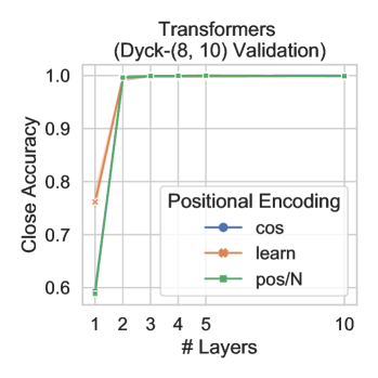
Figure 7: Validation results on $\mathsf{Dyck}_{8,10}$.

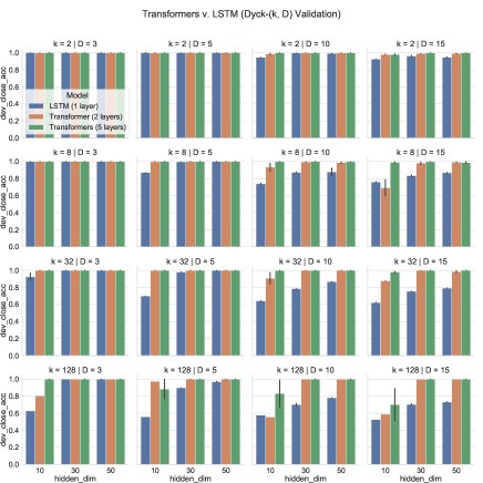
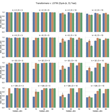
Figure 8: Validation and test results on $\mathsf{Dyck}_{k,D}$ ($k\in\{2,8,32,128\}$ and $D\in\{3,5,10,15\}$). Enlarge for details.

References

- Ba et al. (2016) Jimmy Lei Ba, Jamie Ryan Kiros, and Geoffrey E Hinton. 2016. Layer normalization. arXiv preprint arXiv:1607.06450.
- Bernardy (2018) Jean-Phillipe Bernardy. 2018. Can recurrent neural networks learn nested recursion? In Linguistic Issues in Language Technology, Volume 16, 2018. CSLI Publications.
- Bhattamishra et al. (2020a) Satwik Bhattamishra, Kabir Ahuja, and Navin Goyal. 2020a. On the ability of self-attention networks to recognize counter languages. In Proceedings of the 2020 Conference on Empirical Methods in Natural Language Processing (EMNLP), pages 7096–7116.
- Bhattamishra et al. (2020b) Satwik Bhattamishra, Arkil Patel, and Navin Goyal. 2020b. On the computational power of transformers and its implications in sequence modeling. In Proceedings of the 24th Conference on Computational Natural Language Learning, pages 455–475, Online. Association for Computational Linguistics.
- Brennan and Hale (2019) Jonathan R Brennan and John T Hale. 2019. Hierarchical structure guides rapid linguistic predictions during naturalistic listening. PloS one, 14(1):e0207741.
- Chen et al. (2018) Mia Xu Chen, Orhan Firat, Ankur Bapna, Melvin Johnson, Wolfgang Macherey, George Foster, Llion Jones, Mike Schuster, Noam Shazeer, Niki Parmar, Ashish Vaswani, Jakob Uszkoreit, Lukasz Kaiser, Zhifeng Chen, Yonghui Wu, and Macduff Hughes. 2018. The best of both worlds: Combining recent advances in neural machine translation. In Proceedings of the 56th Annual Meeting of the Association for Computational Linguistics (Volume 1: Long Papers), pages 76–86, Melbourne, Australia. Association for Computational Linguistics.
- Chomsky (1956) Noam Chomsky. 1956. Three models for the description of language. IRE Transactions on information theory, 2(3):113–124.
- Chomsky and Schützenberger (1959) Noam Chomsky and Marcel P Schützenberger. 1959. The algebraic theory of context-free languages. In Studies in Logic and the Foundations of Mathematics, volume 26, pages 118–161. Elsevier.
- Das et al. (1992) Sreerupa Das, C Lee Giles, and Guo-Zheng Sun. 1992. Learning context-free grammars: Capabilities and limitations of a recurrent neural network with an external stack memory. In Proceedings of The Fourteenth Annual Conference of Cognitive Science Society. Indiana University, page 14. Citeseer.
- Dehghani et al. (2019) Mostafa Dehghani, Stephan Gouws, Oriol Vinyals, Jakob Uszkoreit, and Lukasz Kaiser. 2019. Universal transformers. In 7th International Conference on Learning Representations, ICLR 2019, New Orleans, LA, USA, May 6-9, 2019. OpenReview.net.
- Ebrahimi et al. (2020) Javid Ebrahimi, Dhruv Gelda, and Wei Zhang. 2020. How can self-attention networks recognize Dyck-n languages? In Findings of the Association for Computational Linguistics: EMNLP 2020, pages 4301–4306, Online. Association for Computational Linguistics.
- Elman (1990) Jeffrey L Elman. 1990. Finding structure in time. Cognitive science, 14(2):179–211.
- Frank et al. (2012) Stefan L Frank, Rens Bod, and Morten H Christiansen. 2012. How hierarchical is language use? Proceedings of the Royal Society B: Biological Sciences, 279(1747):4522–4531.
- Frank and Christiansen (2018) Stefan L Frank and Morten H Christiansen. 2018. Hierarchical and sequential processing of language: A response to: Ding, melloni, tian, and poeppel (2017). rule-based and word-level statistics-based processing of language: insights from neuroscience. language, cognition and neuroscience. Language, Cognition and Neuroscience, 33(9):1213–1218.
- Hahn (2020) Michael Hahn. 2020. Theoretical limitations of self-attention in neural sequence models. Transactions of the Association for Computational Linguistics, 8:156–171.
- Hao et al. (2019) Jie Hao, Xing Wang, Baosong Yang, Longyue Wang, Jinfeng Zhang, and Zhaopeng Tu. 2019. Modeling recurrence for transformer. In Proceedings of the 2019 Conference of the North American Chapter of the Association for Computational Linguistics: Human Language Technologies, Volume 1 (Long and Short Papers), pages 1198–1207, Minneapolis, Minnesota. Association for Computational Linguistics.
- Hauser et al. (2002) Marc D Hauser, Noam Chomsky, and W Tecumseh Fitch. 2002. The faculty of language: what is it, who has it, and how did it evolve? science, 298(5598):1569–1579.
- He and Choi (2019) Han He and Jinho D Choi. 2019. Establishing strong baselines for the new decade: Sequence tagging, syntactic and semantic parsing with bert. arXiv preprint arXiv:1908.04943.
- He et al. (2016) Kaiming He, Xiangyu Zhang, Shaoqing Ren, and Jian Sun. 2016. Deep residual learning for image recognition. In 2016 IEEE Conference on Computer Vision and Pattern Recognition, CVPR 2016, Las Vegas, NV, USA, June 27-30, 2016, pages 770–778. IEEE Computer Society.
- Hewitt et al. (2020) John Hewitt, Michael Hahn, Surya Ganguli, Percy Liang, and Christopher D. Manning. 2020. RNNs can generate bounded hierarchical languages with optimal memory. In Proceedings of the 2020 Conference on Empirical Methods in Natural Language Processing (EMNLP), pages 1978–2010, Online. Association for Computational Linguistics.
- Hochreiter and Schmidhuber (1997) Sepp Hochreiter and Jürgen Schmidhuber. 1997. Long short-term memory. Neural computation, 9(8):1735–1780.
- Jin et al. (2018) Lifeng Jin, Finale Doshi-Velez, Timothy Miller, William Schuler, and Lane Schwartz. 2018. Unsupervised grammar induction with depth-bounded PCFG. Transactions of the Association for Computational Linguistics, 6:211–224.
- Karlsson (2007) Fred Karlsson. 2007. Constraints on multiple center-embedding of clauses. Journal of Linguistics, pages 365–392.
- Ke et al. (2021) Guolin Ke, Di He, and Tie-Yan Liu. 2021. Rethinking the positional encoding in language pre-training. In International Conference on Learning Representations, (ICLR 2021).
- Korsky and Berwick (2019) Samuel A Korsky and Robert C Berwick. 2019. On the computational power of rnns. arXiv preprint arXiv:1906.06349.
- Levinson (2014) Stephen C Levinson. 2014. Pragmatics as the origin of recursion. In Language and recursion, pages 3–13. Springer.
- Lin et al. (2019) Yongjie Lin, Yi Chern Tan, and Robert Frank. 2019. Open sesame: Getting inside BERT’s linguistic knowledge. In Proceedings of the 2019 ACL Workshop BlackboxNLP: Analyzing and Interpreting Neural Networks for NLP, pages 241–253, Florence, Italy. Association for Computational Linguistics.
- Manning et al. (2020) Christopher D Manning, Kevin Clark, John Hewitt, Urvashi Khandelwal, and Omer Levy. 2020. Emergent linguistic structure in artificial neural networks trained by self-supervision. Proceedings of the National Academy of Sciences, 117(48):30046–30054.
- Merity et al. (2017) Stephen Merity, Caiming Xiong, James Bradbury, and Richard Socher. 2017. Pointer sentinel mixture models. In 5th International Conference on Learning Representations, ICLR 2017, Toulon, France, April 24-26, 2017, Conference Track Proceedings. OpenReview.net.
- Merrill et al. (2020) William Merrill, Gail Weiss, Yoav Goldberg, Roy Schwartz, Noah A. Smith, and Eran Yahav. 2020. A formal hierarchy of RNN architectures. In Proceedings of the 58th Annual Meeting of the Association for Computational Linguistics, pages 443–459, Online. Association for Computational Linguistics.
- Nelson et al. (2017) Matthew J Nelson, Imen El Karoui, Kristof Giber, Xiaofang Yang, Laurent Cohen, Hilda Koopman, Sydney S Cash, Lionel Naccache, John T Hale, Christophe Pallier, et al. 2017. Neurophysiological dynamics of phrase-structure building during sentence processing. Proceedings of the National Academy of Sciences, 114(18):E3669–E3678.
- Papadimitriou and Jurafsky (2020) Isabel Papadimitriou and Dan Jurafsky. 2020. Learning Music Helps You Read: Using transfer to study linguistic structure in language models. In Proceedings of the 2020 Conference on Empirical Methods in Natural Language Processing (EMNLP), pages 6829–6839, Online. Association for Computational Linguistics.
- Pérez et al. (2019) Jorge Pérez, Javier Marinkovic, and Pablo Barceló. 2019. On the turing completeness of modern neural network architectures. In 7th International Conference on Learning Representations, ICLR 2019, New Orleans, LA, USA, May 6-9, 2019. OpenReview.net.
- Radford et al. (2019) Alec Radford, Jeffrey Wu, Rewon Child, David Luan, Dario Amodei, and Ilya Sutskever. 2019. Language models are unsupervised multitask learners. OpenAI blog, 1(8):9.
- Rahimi and Recht (2007) Ali Rahimi and Benjamin Recht. 2007. Random features for large-scale kernel machines. In Advances in Neural Information Processing Systems 20, Proceedings of the Twenty-First Annual Conference on Neural Information Processing Systems, Vancouver, British Columbia, Canada, December 3-6, 2007, pages 1177–1184. Curran Associates, Inc.
- Sennhauser and Berwick (2018) Luzi Sennhauser and Robert Berwick. 2018. Evaluating the ability of LSTMs to learn context-free grammars. In Proceedings of the 2018 EMNLP Workshop BlackboxNLP: Analyzing and Interpreting Neural Networks for NLP, pages 115–124, Brussels, Belgium. Association for Computational Linguistics.
- Shaw et al. (2018) Peter Shaw, Jakob Uszkoreit, and Ashish Vaswani. 2018. Self-attention with relative position representations. In Proceedings of the 2018 Conference of the North American Chapter of the Association for Computational Linguistics: Human Language Technologies, Volume 2 (Short Papers), pages 464–468, New Orleans, Louisiana. Association for Computational Linguistics.
- Shen et al. (2018) Tao Shen, Tianyi Zhou, Guodong Long, Jing Jiang, Shirui Pan, and Chengqi Zhang. 2018. Disan: Directional self-attention network for rnn/cnn-free language understanding. In Proceedings of the Thirty-Second AAAI Conference on Artificial Intelligence, (AAAI-18), the 30th innovative Applications of Artificial Intelligence (IAAI-18), and the 8th AAAI Symposium on Educational Advances in Artificial Intelligence (EAAI-18), New Orleans, Louisiana, USA, February 2-7, 2018, pages 5446–5455. AAAI Press.
- Shiv and Quirk (2019) Vighnesh Leonardo Shiv and Chris Quirk. 2019. Novel positional encodings to enable tree-based transformers. In Advances in Neural Information Processing Systems 32: Annual Conference on Neural Information Processing Systems 2019, NeurIPS 2019, December 8-14, 2019, Vancouver, BC, Canada, pages 12058–12068.
- Steijvers and Grünwald (1996) Mark Steijvers and Peter Grünwald. 1996. A recurrent network that performs a context-sensitive prediction task. In Proceedings of the 18th annual conference of the cognitive science society, pages 335–339.
- Suzgun et al. (2019) Mirac Suzgun, Sebastian Gehrmann, Yonatan Belinkov, and Stuart M Shieber. 2019. Memory-augmented recurrent neural networks can learn generalized dyck languages. arXiv preprint arXiv:1911.03329.
- Tenney et al. (2019) Ian Tenney, Dipanjan Das, and Ellie Pavlick. 2019. BERT rediscovers the classical NLP pipeline. In Proceedings of the 57th Annual Meeting of the Association for Computational Linguistics, pages 4593–4601, Florence, Italy. Association for Computational Linguistics.
- Tran et al. (2018) Ke Tran, Arianna Bisazza, and Christof Monz. 2018. The importance of being recurrent for modeling hierarchical structure. In Proceedings of the 2018 Conference on Empirical Methods in Natural Language Processing, pages 4731–4736, Brussels, Belgium. Association for Computational Linguistics.
- Vaswani et al. (2017) Ashish Vaswani, Noam Shazeer, Niki Parmar, Jakob Uszkoreit, Llion Jones, Aidan N. Gomez, Lukasz Kaiser, and Illia Polosukhin. 2017. Attention is all you need. In Advances in Neural Information Processing Systems 30: Annual Conference on Neural Information Processing Systems 2017, December 4-9, 2017, Long Beach, CA, USA, pages 5998–6008.
- Wang et al. (2020) Benyou Wang, Donghao Zhao, Christina Lioma, Qiuchi Li, Peng Zhang, and Jakob Grue Simonsen. 2020. Encoding word order in complex embeddings. In 8th International Conference on Learning Representations, ICLR 2020, Addis Ababa, Ethiopia, April 26-30, 2020. OpenReview.net.
- Wolf et al. (2019) Thomas Wolf, Lysandre Debut, Victor Sanh, Julien Chaumond, Clement Delangue, Anthony Moi, Pierric Cistac, Tim Rault, Rémi Louf, Morgan Funtowicz, et al. 2019. Huggingface’s transformers: State-of-the-art natural language processing. arXiv preprint arXiv:1910.03771.
- Yang et al. (2019) Baosong Yang, Longyue Wang, Derek F. Wong, Lidia S. Chao, and Zhaopeng Tu. 2019. Assessing the ability of self-attention networks to learn word order. In Proceedings of the 57th Annual Meeting of the Association for Computational Linguistics, pages 3635–3644, Florence, Italy. Association for Computational Linguistics.
- Yu et al. (2019) Xiang Yu, Ngoc Thang Vu, and Jonas Kuhn. 2019. Learning the Dyck language with attention-based Seq2Seq models. In Proceedings of the 2019 ACL Workshop BlackboxNLP: Analyzing and Interpreting Neural Networks for NLP, pages 138–146, Florence, Italy. Association for Computational Linguistics.
- Yun et al. (2020) Chulhee Yun, Srinadh Bhojanapalli, Ankit Singh Rawat, Sashank J. Reddi, and Sanjiv Kumar. 2020. Are transformers universal approximators of sequence-to-sequence functions? In 8th International Conference on Learning Representations, ICLR 2020, Addis Ababa, Ethiopia, April 26-30, 2020. OpenReview.net.
- Zhang et al. (2020) Yu Zhang, Houquan Zhou, and Zhenghua Li. 2020. Fast and accurate neural CRF constituency parsing. In Proceedings of the Twenty-Ninth International Joint Conference on Artificial Intelligence, IJCAI 2020, pages 4046–4053. ijcai.org.