Complex Langevin study for polarons in an attractively interacting one-dimensional two-component Fermi gas

Abstract

We investigate a polaronic excitation in a one-dimensional spin-1/2 Fermi gas with contact attractive interactions, using the complex Langevin method, which is a promising approach to evade a possible sign problem in quantum Monte Carlo simulations. We found that the complex Langevin method works correctly in a wide range of temperature, interaction strength, and population imbalance. The Fermi polaron energy extracted from the two-point imaginary Green’s function is not sensitive to the temperature and the impurity concentration in the parameter region we considered. Our results show a good agreement with the solution of the thermodynamic Bethe ansatz at zero temperature.

I Introduction

The quantum Monte Carlo method von der Linden (1992); Pollet (2012) is widely used in various fields of physics as a non-perturbative tool of analysis. In a path integral formalism using Lagrangian, a partition function is written in terms of the integral of the Boltzmann weight $\mathrm{e}^{-S}$ over field variables, where $S$ is an action. When the action is a real-valued function, the Boltzmann weight is regarded as a probability density function. This ensures that quantum expectation values of physical observables can be estimated by importance sampling of the Boltzmann weight. However, the positivity of the Boltzmann weight is violated in many physically interesting systems: Hubbard model, finite density quantum chromodynamics (QCD), QCD with a $\theta$-term, matrix superstring models and any systems defined by Schwinger-Keldysh formalism which describes real-time dynamics, for instance Loh et al. (1990); Troyer and Wiese (2005); Muroya et al. (2003); de Forcrand (2009); Vicari and Panagopoulos (2009); Krauth et al. (1998); Berges et al. (2007); Alexandru et al. (2016). In these cases, the number of samples becomes exponentially large as the system size grows in order to obtain statistically significant results. In non-relativistic fermionic systems, a frequently used way to apply the quantum Monte Carlo method is introducing bosonic auxiliary field through the Hubbard-Stratonovich transformation Blankenbecler et al. (1981); Scalapino and Sugar (1981); Sugiyama and Koonin (1986). After integrating out the fermion fields, we will obtain an effective action of the auxiliary field. Since the effective action involves a logarithm of a fermion determinant, the positivity is not guaranteed except in a few cases where the action has the particle-hole symmetry Hirsch (1985), the Kramers symmetry Wu and Zhang (2005), or Majorana positivity Li et al. (2015, 2016); Wei et al. (2016), for instance.

A promising approach to evade the sign problem is the complex Langevin method Klauder (1984); Parisi (1983), which is an extension of the stochastic quantization to systems with complex-valued actions. An advantage of this method is that it is scalable to the system size, and thus, the computational cost is similar to the usual quantum Monte Carlo method without the sign problem. On the other hand, it is known that this method sometimes gives incorrect answers even when the statistical average of a physical observable converges. In the recent decade, a way to judge the reliability of the complex Langevin method is extensively studied Aarts et al. (2010, 2011); Nishimura and Shimasaki (2015); Nagata et al. (2016a, b); Salcedo (2016); Aarts et al. (2017); Nagata et al. (2018); Scherzer et al. (2019, 2020); Cai et al. (2021), and proposed criteria which are able to compute in actual simulations using the boundary terms Aarts et al. (2010, 2011); Scherzer et al. (2019, 2020) and the probability distribution of the drift term Nishimura and Shimasaki (2015); Nagata et al. (2016b). While it is still difficult to predict when the complex Langevin method fails without performing numerical simulations, we can eliminate wrongly convergent results thanks to these criteria. In the context of cold fermionic atoms, the complex Langevin method is applied to rotating bosons Hayata and Yamamoto (2015), polarized fermions Loheac et al. (2018); Rammelmüller et al. (2018, 2020, 2021), unpolarized fermions with contact repulsive interactions Loheac and Drut (2017) and mass imbalanced fermions Rammelmüller et al. (2017) to study ground state energy, thermodynamic quantities and Fulde-Ferrell-Larkin-Ovchinnikov-type pairings (see also a recent review Berger et al. (2021)).

In this paper, we consider a spatially one-dimensional spin-1/2 polarized fermions with contact attractive interactions which is known as the Gaudin-Yang model Guan et al. (2013), and compute the single-particle energy of spin-down fermions in a spin-up Fermi sea, which is referred to as the Fermi polaron energy. Recently, the single-particle excitation spectra of Fermi polarons were experimentally measured in higher dimensional atomic systems Schirotzek et al. (2009); Nascimbène et al. (2009); Koschorreck et al. (2012); Cetina et al. (2016); Scazza et al. (2017); Adlong et al. (2020); Ness et al. (2020); Fritsche et al. (2021) (also see a recent review Massignan et al. (2014) for Fermi polarons). While an analytic formula for the polaron energy in one dimension is obtained exactly at zero temperature based on the thermodynamic Bethe ansatz method McGuire (1966), no analytical solutions are known at finite temperature (note that the numerical results for finite-temperature properties of polarized gases within the thermodynamic Bethe ansatz were reported in Ref. He et al. (2016)). The one-dimensional Fermi polarons were studied with several theoretical approaches such as Bruckner-Hartree-Fock Klawunn and Recati (2011), T-matrix Doggen and Kinnunen (2013); Tajima et al. (2021), and variational S. Yadong and Z. Huawen (2019); Mistakidis et al. (2019) approaches. In this study, we demonstrate that a microscopic quantity, that is, the polaron energy is efficiently computed by the complex Langevin method.

This paper is organized as follows. In Sec. II, we derive a lattice action of the Gaugin-Yang model. In Sec. III, we review how to compute physical quantities using the complex Langevin method. In Sec. IV, we show a way to extract the ground state energy in the spin-down channel from a two-point imaginary time Green’s function. In Sec. V, we present the numerical results. Section VI is devoted to the summary of this paper. In this work, $k_{\rm B}$ and $\hbar$ are taken to be unity.

II The Gaudin-Yang model

We consider a one-dimensional two-component Fermi gas with contact attractive interactions which is known as the Gaugin-Yang model Yang (1967); Gaudin (1967). The Hamiltonian is given by

$$\hat{H}=\sum_{p,\sigma}\quantity(\frac{p^{2}}{2}-\mu_{\sigma})\hat{c}_{p,\sigma}^{\dagger}\hat{c}_{p,\sigma}-g\sum_{p,p^{\prime},q}\hat{c}_{p+\frac{q}{2},\uparrow}^{\dagger}\hat{c}_{-p+\frac{q}{2},\downarrow}^{\dagger}\hat{c}_{-p^{\prime}+\frac{q}{2},\downarrow}\hat{c}_{p^{\prime}+\frac{q}{2},\uparrow},$$ (1)

where $\hat{c}_{p,\sigma}$ and $\hat{c}_{p,\sigma}^{{\dagger}}$ are fermionic annihilation/creation operators with momentum $p$ and spin $\sigma=\uparrow,\downarrow$, respectively. In this work, the atomic mass is taken to be unity. The coupling constant $g$ is related to a scattering length in one dimension $a$ as $g=\frac{2}{a}>0$ Guan et al. (2013). The chemical potential of spin-$\sigma$ fermions are represented by $\mu_{\sigma}$. For convenience, we introduce an average chemical potential $\mu=(\mu_{\uparrow}+\mu_{\downarrow})/2$ and a fictitious Zeeman field $h=(\mu_{\uparrow}-\mu_{\downarrow})/2$. The grand canonical partition function is given by $Z=\Tr\bqty{\mathrm{e}^{-\beta\quantity(\hat{H}-\sum_{\sigma}\mu_{\sigma}\hat{N}_{\sigma})}}$ with $\beta$ being an inverse temperature and a number operator $\hat{N}_{\sigma}=\sum_{p}\hat{c}_{p,\sigma}^{\dagger}\hat{c}_{p,\sigma}$. The path-integral representation of $Z$ reads

$$Z=\int\prod_{\sigma}\mathcal{D}\psi^{*}_{\sigma}\mathcal{D}\psi_{\sigma}\ \mathrm{e}^{-S},$$ (2)

where action $S$ is given by

$$S=\int_{0}^{\beta}\differential{\tau}\int\differential{x}\Bigg{[} \sum_{\sigma=\uparrow,\downarrow}\psi^{*}_{\sigma}(x,\tau)\quantity(\frac{\partial}{\partial\tau}-\frac{1}{2}\frac{\partial^{2}}{\partial x^{2}}-\mu_{\sigma})\psi_{\sigma}(x,\tau)$$

$$\qquad\qquad-g\psi^{*}_{\uparrow}(x,\tau)\psi^{*}_{\downarrow}(x,\tau)\psi_{\downarrow}(x,\tau)\psi_{\uparrow}(x,\tau)\Bigg{]}.$$ (3)

Here $\psi_{\sigma}(x,\tau),\psi^{*}_{\sigma}(x,\tau)$ are a Grassmann field and its complex conjugate.

While the action (3) is given in a continuous spacetime, one should perform a lattice regularization appropriately to carry out numerical simulations. We write lattice spacing of temporal and spatial directions by $a_{\tau}$ and $a_{x}$, respectively, and their ratio by $r=a_{\tau}/a_{x}^{2}$. We also introduce lattice quantities by

$$\bar{\mu}_{\sigma}\equiv\mu_{\sigma}a_{x}^{2},\quad\bar{g}\equiv ga_{x},\quad\bar{\psi}_{\sigma,j,n}\equiv\psi_{\sigma}(ja_{x},na_{\tau})a_{x}^{1/2},$$ (4)

where $n$ and $j$ are integers that satisfy $0\leq n<N_{\tau}$ and $0\leq j<N_{x}$. The inverse temperature and the spatial length of the lattice is given by $\beta=T^{-1}=N_{\tau}a_{\tau}$ and $L=N_{x}a_{x}$. With these notations, we consider a lattice action:

$$S_{\text{lat}}= \sum_{j,n}\sum_{\sigma=\uparrow,\downarrow}\quantity(\bar{\psi}^{*}_{\sigma;j,n}\bar{\psi}_{\sigma;j,n}-\bar{\psi}^{*}_{\sigma;j,n+1}e^{-\bar{\phi}_{j,n}+\bar{\mu}_{\sigma}}\bar{\psi}_{\sigma;j,n}+\frac{r}{2}(\bar{\psi}^{*}_{\sigma;j+1,n}-\bar{\psi}^{*}_{\sigma;j,n})(\bar{\psi}_{\sigma;j+1,n}-\bar{\psi}_{\sigma;j,n}))$$

$$+\sum_{j,n}\frac{\cosh(\bar{\phi}_{j,n})-1}{\bar{g}},$$ (5)

where $\bar{\phi}_{j,n}$ is a bosonic auxiliary field. As shown in Ref. Alexandru et al. (2018), the lattice action (5) correctly converges to the continuum one as long as the matching conditions

$$\frac{ga_{\tau}}{a_{x}}=\quantity(\frac{f_{2}}{f_{0}}-\frac{f_{1}^{2}}{f_{0}^{2}})\mathrm{e}^{\bar{\mu}_{\uparrow}+\bar{\mu}_{\downarrow}},\quad\mu_{\sigma}a_{\tau}=\frac{f_{1}}{f_{0}}\mathrm{e}^{\bar{\mu}_{\sigma}}-1$$ (6)

are satisfied, where $f_{k}$ is a $\bar{g}$-dependent constant given by

$$f_{k}=\int_{-\infty}^{\infty}\differential{\bar{\phi}}\mathrm{e}^{-\frac{\cosh(\bar{\phi})-1}{\bar{g}}}\mathrm{e}^{k\bar{\phi}}.$$ (7)

In practice, it is sufficient to use an approximated form of the matching conditions

$$\bar{g}\simeq\frac{ga_{\tau}}{a_{x}},\quad\bar{\mu}_{\sigma}\simeq\mu_{\sigma}a_{\tau}-\frac{ga_{\tau}}{2a_{x}},$$ (8)

which are obtained as the first order approximation in the expansion in terms of $a_{\tau}$. After integrating out the fermion fields, the partition function and the effective action of the auxiliary field read

$$Z =\int\prod_{j,n}\differential{\bar{\phi}_{j,n}}\mathrm{e}^{-S_{\text{eff}}[\bar{\phi}]},$$ (9)

where the effective action of the auxiliary field is given by

$$S_{\text{eff}}[\bar{\phi}] =\sum_{j,n}\frac{\cosh\bar{\phi}_{j,n}-1}{\bar{g}}-\sum_{\sigma}\log\det\quantity[I+e^{N_{\tau}\bar{\mu}_{\sigma}}B^{-1}C_{N_{\tau}-1}\cdots B^{-1}C_{0}],$$ (10)

$$B_{j,j^{\prime}} =-\frac{r}{2}\quantity(\delta_{j-1,j^{\prime}}+\delta_{j+1,j^{\prime}})+\quantity(1+r)\delta_{j,j^{\prime}},\quad(C_{n})_{j,j^{\prime}}=\delta_{j,j^{\prime}}e^{-\bar{\phi}_{j,n}},$$ (11)

where $I$ is the $N_{x}\times N_{x}$ identity matrix. Since we consider a naive finite difference as an approximation of the second order derivative with respect to $x$, the eigenvalues of $B$ are $1+2r\sin^{2}\frac{\pi k}{N_{x}},(k=0,1,\cdots,N_{x}-1)$. It has been argued in Ref. Blankenbecler et al. (1981); Alexandru et al. (2018) that this naive lattice action converges too slow to the continuum limit, and the behavior can be improved by replacing the eigenvalues of $B$ by

$$\lambda_{k}=\exp(\frac{r}{2}\quantity(\frac{2\pi k}{N_{x}})^{2}).$$ (12)

After this replacement, the form of $B_{\sigma}$ is given by

$$B_{j,j^{\prime}}=\frac{1}{N_{x}}\sum_{k=-\lfloor N_{x}/2\rfloor}^{\lfloor N_{x}/2\rfloor}\lambda_{k}\cos k(j-j^{\prime}).$$ (13)

A notable point is that the effective action (10) involves a logarithm of the fermion determinant which can be complex in general. Therefore, this term may cause the sign problem if the Zeeman field $h$ is not zero and then the Monte Carlo simulation can be difficult to apply to this system.

III Complex Langevin method

The complex Langevin method (CLM) Klauder (1984); Parisi (1983) is an extension of the stochastic quantization which is usually applicable to real-valued actions. In the CLM, we first consider a complexified auxiliary field $\bar{\phi}_{n,k}$ and extend the domain of definition of $S_{\text{eff}}$ to the complex space. For such a complex field, we consider a fictitious time evolution described by the complex Langevin equation:

$$\bar{\phi}^{\eta}_{n,k}(t+\Delta t)=\bar{\phi}^{\eta}_{n,k}(t)-\frac{\partial S_{\text{eff}}}{\partial\bar{\phi}^{\eta}_{n,k}}\Delta t+\eta_{n,k}(t)\sqrt{\Delta t},$$ (14)

where $\eta_{n,k}(t)$ is a real Gaussian noise. When we assume that the system described by the complex Langevin equation reach equilibrium at $t=t_{\text{eq}}$, an average of a physical observable $O(\bar{\phi})$ can be defined as

$$\expectationvalue{O(\bar{\phi})}\equiv\lim_{T\to\infty}\frac{1}{T}\int_{t_{\text{eq}}}^{t_{\text{eq}}+T}\differential{t}\expectationvalue{O(\bar{\phi}^{\eta}(t))}_{\eta},$$ (15)

with the average over the noise $\expectationvalue{O(\bar{\phi}^{\eta}(t))}_{\eta}$ being

$$\expectationvalue{O(\bar{\phi}^{\eta}(t))}_{\eta}\equiv\frac{\int\prod_{n,k,t}\differential{\eta}_{n,k}(t)O(\bar{\phi}^{\eta}(t))\mathrm{e}^{-\frac{1}{4}\sum_{n,k,t}\eta_{n,k}(t)^{2}}}{\int\prod_{n,k,t}\differential{\eta}_{n,k}(t)\mathrm{e}^{-\frac{1}{4}\sum_{n,k,t}\eta_{n,k}(t)^{2}}}.$$ (16)

We note that $\expectationvalue{\eta_{n,k}(t)\eta_{n^{\prime},k^{\prime}}(t^{\prime})}_{\eta}=2\delta_{nn^{\prime}}\delta_{kk^{\prime}}\delta_{tt^{\prime}}$, in particular. Although, we expect that the mean value $\expectationvalue{O(\bar{\phi})}$ is equivalent to the quantum expectation value calculated in an original action, i.e., $\int\prod_{n,k}\differential{\bar{\phi}}_{n,k}O(\bar{\phi})\mathrm{e}^{-S_{\text{eff}}}/\int\prod_{n,k}\differential{\bar{\phi}}_{n,k}\mathrm{e}^{-S_{\text{eff}}}$ in the limit $\Delta t\to 0$, it is not correct in general. There are extensive studies Aarts et al. (2010, 2011); Nishimura and Shimasaki (2015); Nagata et al. (2016a, b); Salcedo (2016); Aarts et al. (2017); Nagata et al. (2018); Scherzer et al. (2019, 2020); Cai et al. (2021) to understand when the CLM is justified, and criteria for determining whether a CLM is reliable or not have been proposed. One of a practical criterion which can be relied on in actual numerical simulations is discussed from a view point of a probability distribution of a drift term Nishimura and Shimasaki (2015); Nagata et al. (2016b). In our case, it is sufficient to consider a magnitude of the drift term given by

$$v^{\eta}\equiv\max_{n,k}\quantity|\frac{\partial S_{\text{eff}}}{\partial\bar{\phi}^{\eta}_{n,k}}|$$ (17)

and its distribution. According to the criterion, the CLM is reliable if the probability distribution of $v^{\eta}$ shows an exponential decay.

IV Observables

The number density of spin-$\sigma$ fermions is given by

$$n_{\sigma}=\frac{T}{L}\frac{\partial}{\partial\mu_{\sigma}}\log Z=\frac{1}{L}\frac{1}{Z}\int\prod_{j,n}\differential{\bar{\phi}_{j,n}}\tr\quantity[\frac{1}{I+e^{-N_{\tau}\bar{\mu}_{\sigma}}C_{0}^{-1}B\cdots C_{N_{\tau}-1}^{-1}B}]\mathrm{e}^{-S_{\text{eff}}[\bar{\phi}]}.$$ (18)

The particle number density on a lattice unit is defined by $\bar{n}_{\sigma}=n_{\sigma}a_{x}$. From below, we assume that the spin-down fermions are regarded as minority. Typical temperature and momentum scales are given by the Fermi scales which are determined by the density of spin-up fermions:

$$T_{\text{F}}=\frac{\pi^{2}n_{\uparrow}}{2},\quad p_{\text{F}}=\pi n_{\uparrow}.$$ (19)

In lattice simulations, we can compute dimensionless combination $T/T_{\text{F}}$ and $p_{\text{F}}a$ as follows:

$$\frac{T}{T_{\text{F}}}=\frac{2}{\pi^{2}\bar{n}_{\uparrow}^{2}N_{\tau}r},\quad p_{\text{F}}a=\frac{2\pi r\bar{n}_{\uparrow}}{\bar{g}}.$$ (20)

In order to calculate the polaron energy, we consider two-point Green’s function:

$$G(p,\tau)\equiv\frac{1}{Z}\Tr[e^{-\beta\hat{K}}\operatorname{\mathrm{T}}_{\tau}\quantity(\hat{c}^{\dagger}_{\downarrow,p}(\tau)\hat{c}_{\downarrow,0}(0))],\quad(-\beta\leq\tau\leq\beta),$$ (21)

where $\operatorname{\mathrm{T}}_{\tau}$ is the imaginary-time-ordered product. Hereinafter we restrict $\tau>0$. We write the eigenvalue and eigenstate of $\hat{K}$ by $\hat{K}\ket{n}=K_{n}\ket{n}$. In particular, $K_{0}<K_{1}<\cdots$. We also assume that the ground state $\ket{0}$ is not degenerated. Expanding the trace by the eigenstates, the correlation function reads

$$G(p,\tau)=\frac{\sum_{nm}e^{-(\beta-\tau)\Delta K_{n}-\tau\Delta K_{m}}\matrixelement{n}{\hat{c}^{\dagger}_{\sigma,p}}{m}\matrixelement{m}{\hat{c}_{\sigma^{\prime},p^{\prime}}}{n}}{\sum_{n}e^{-\beta\Delta K_{n}}},$$ (22)

where $\Delta K_{n}\equiv K_{n}-K_{0}$. In the low temperature limit $\beta\to\infty$, only the ground state contributes to the summation over $n$. Thus, we find

$$\tilde{G}(p,\tau)\equiv\lim_{\beta\to\infty}G(p,\tau)=\sum_{m}e^{-\tau\Delta K_{m}}\matrixelement{0}{\hat{c}^{\dagger}_{\sigma,p}}{m}\matrixelement{m}{\hat{c}_{\sigma^{\prime},p^{\prime}}}{0}.$$ (23)

Since the matrix elements appeared in the above expression does not depend on $\tau$, it behaves like

$$\tilde{G}(p,\tau)=A_{0}e^{-\tau E_{0}}+A_{1}e^{-\tau E_{1}}+\dots,$$ (24)

where $A_{0},A_{1},\dots$ are $\tau$-independent constants, and $E_{0},E_{1},\dots$ are energies of the ground state and excited states. In particular, the energy of the ground state can be extracted by

$$E_{0}(p)=\frac{1}{a_{\tau}}\lim_{\tau\to\infty}R(p,\tau),\quad R(p,\tau)\equiv\log\frac{\tilde{G}(p,\tau)}{\tilde{G}(p,\tau+a_{\tau})},$$ (25)

keeping $\tau\ll\beta$. The polaron energy $U$ is defined by

$$U\equiv E_{0}(0)+\mu_{\downarrow}.$$ (26)

The polaron energy is the shift of single-particle energy from that in the case of free fermions due to the interaction between majority (spin-up fermions) and minority (spin-down fermions). We note that the polaron energy at zero temperature is calculated exactly based on thermodynamic Bethe ansatz McGuire (1966):

$$\frac{U}{T_{\text{F}}}=-\frac{2}{\pi}\quantity[\frac{1}{p_{\text{F}}a}+\tan^{-1}\quantity(\frac{1}{p_{\text{F}}a})+\quantity(\frac{\pi}{2}+\tan^{-1}\quantity(\frac{1}{p_{\text{F}}a}))\frac{1}{(p_{\text{F}}a)^{2}}].$$ (27)

In lattice calculations, the polaron energy is obtained as follows. From the form of the effective action, the lattice expression of the inverse Green’s function reads

$$G^{-1}\equiv\begin{pmatrix}B&0&0&\cdots&0&\mathrm{e}^{\bar{\mu}_{\downarrow}}C_{N_{\tau}-1}\\ -\mathrm{e}^{\bar{\mu}_{\downarrow}}C_{0}&B&0&\cdots&0&0\\ 0&-\mathrm{e}^{\bar{\mu}_{\downarrow}}C_{1}&B&\cdots&0&0\\ \vdots&\vdots&\vdots&\ddots&\vdots&\vdots\\ 0&0&0&\cdots&-\mathrm{e}^{\bar{\mu}_{\downarrow}}C_{N_{\tau}-2}&B\end{pmatrix}.$$ (28)

From a straightforward algebra, each component of $G$ reads

$$G_{jj} =\frac{B^{-1}}{I+\mathrm{e}^{N_{\tau}\bar{\mu}_{\downarrow}}B^{-1}C_{j-1}\cdots B^{-1}C_{0}B^{-1}C_{N_{\tau}-1}\cdots B^{-1}C_{j}},$$ (29)

$$G_{kj} =\begin{cases}B^{-1}C_{k-1}\cdots B^{-1}C_{j}G_{jj},\quad&(j+1\leq k\leq N-1),\\ -B^{-1}C_{k-1}\cdots B^{-1}C_{0}B^{-1}C_{N-1}\cdots B^{-1}C_{j}G_{jj},\quad&(0\leq k\leq j-1).\end{cases}$$ (30)

The momentum representation of $G_{ij}$ is calculated by the discrete Fourier transformation. Therefore, if the temporal lattice size $N_{\tau}$ is sufficiently large, $\tilde{G}(p,\tau)$ is approximately given by

$$\tilde{G}(2\pi k/N_{x},na_{\tau})\simeq\frac{1}{N_{x}}\sum_{k^{\prime},l^{\prime}=0}^{N_{x}-1}\mathrm{e}^{\frac{2\pi i}{N_{x}}kk^{\prime}}(G_{0n})_{k^{\prime}l^{\prime}}.$$ (31)

V Numerical results

We performed complex Langevin simulations on $(N_{\tau},N_{x})=(40,60),(80,60)$ lattices. The anisotropy is set to $r=0.1$. There are three dimensionless parameters to characterize the Gaugin-Yang model: $\beta\mu$, $\beta h$ and $\lambda\equiv\sqrt{\beta}g$. We fixed the dimensionless coupling constant by $\lambda=2$, and swept the average chemical potential and the Zeeman field between $-1.2\leq\beta\mu\leq 1.2,\,0\leq\beta h\leq 12$ for $N_{\tau}=40$ and $-2.4\leq\beta\mu\leq 2.4,\,0\leq\beta h\leq 24$ for $N_{\tau}=80$, respectively. We set Langevin step-size by $\Delta t=0.01$, and saved configurations of the auxiliary field at the 0.02 interval. For every parameter sets, we took 5001 samples. Error bars shown below are $1\sigma$ statistical errors calculated by the Jackknife method, where bin-sizes are $0.3-1.2$ in units of Langevein time depending on parameters and observables.

In every Langevin step, the magnitude of the drift term (17) is calculated and stored, and finally the probability distribution $P(v^{\eta})$ of drift term can be drown. In Fig. 1, a typical result of the probability distribution $P(v^{\eta})$ is shown. It is normalized so that the integral of the distribution is 1. In each simulation, we confirmed that $P(v^{\eta})$ shows a linear fall-off in the log-log plot. This means that $P(v^{\eta})$ shows an exponential fall-off, and then our calculation of CLM was reliable.

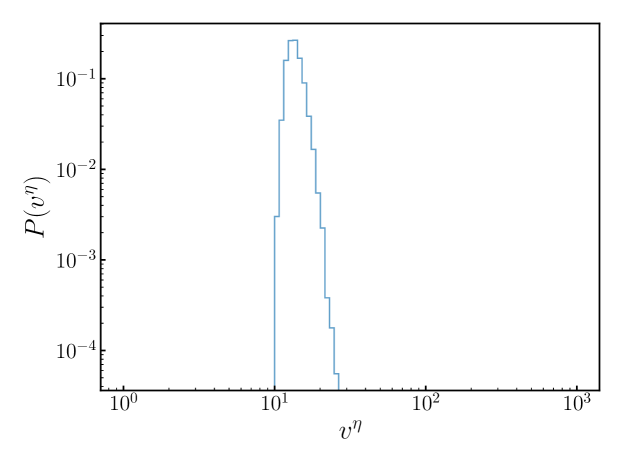
Figure 1: The histogram of the drift term for the $N_{\tau}=40$ lattice at $\beta\mu=0$, $\beta h=3$.

We also investigated the eigenvalues of the matrix

$$G^{-1}_{\sigma,{\rm red}}=I+e^{N_{\tau}\bar{\mu}_{\sigma}}B^{-1}C_{N_{\tau}-1}\cdots B^{-1}C_{0},$$ (32)

which is the reduced matrix of inverse Green’s function Eq. (28) appearing in the effective action on the lattice Eq. (10) as an effective fermionic matrix. We calculate the eigenvalues $w_{\sigma}$ of the matrix from one configuration in the case of several values of $\beta h=0$ to $\beta h=12$ and other fixed parameters, $N_{\tau}=40$ and $\beta\mu=-1.2$. The imaginary part of $w_{\sigma}$ is negligibly small and hereinafter we discuss the real part of the eigenvalues. The numerical results of eigenvalues $\log{\rm Re}[w_{\sigma}]$ of the matrices $G^{-1}_{\uparrow,{\rm red}}$ and $G^{-1}_{\downarrow,{\rm red}}$ are shown in Fig. 2. Red circles and blue squares correspond to the eigenvalues of $G^{-1}_{\uparrow,{\rm red}}$ and $G^{-1}_{\downarrow,{\rm red}}$, respectively. In the case of $\beta h=0$, $w_{\uparrow}$ is exactly same as $w_{\downarrow}$ because $G^{-1}_{\uparrow,{\rm red}}=G^{-1}_{\downarrow,{\rm red}}$. While the range of the eigenvalues of $G^{-1}_{\uparrow,{\rm red}}$ tend to be broad, the range of the eigenvalues of $G^{-1}_{\downarrow,{\rm red}}$ tend to be narrow when $\beta h$ increases.

It is notable point of this eigenvalue-analysis that the eigenvalues of $G^{-1}_{\sigma,{\rm red}}$ are always larger than 1 because of $\log({\rm Re}[w])>0$ even in the case of the large $\beta h$, corresponding to the large population imbalance. This result indicates that the integrand of the partition function (9) is always positive and no sign problem happens in the parameter region of our calculations. Note that this is a numerical finding in our setup, and we do not prove that the sign problem never occurs in the Gaudin-Yang model with population imbalance. We note that the sign problem may occur in other situations within the Hamiltonian (1) or the action (3), for example, considering other values of masses, chemical potentials, coupling constants, lattice parameters, and dimensions.

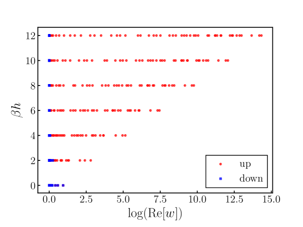
Figure 2: The eigenvalues of matrix $G^{-1}_{\sigma,{\rm red}}$ with several values of $h$ in the case of $N_{\tau}=40$ and $\beta\mu=-1.2$. Red circles and blue squares correspond to $G^{-1}_{\uparrow,{\rm red}}$ and $G^{-1}_{\downarrow,{\rm red}}$, respectively.

In Fig. 3, we show dimensionless quantities $T/T_{\text{F}}$, $1/p_{\text{F}}a$ and $n_{\downarrow}/n_{\uparrow}$, which are typical indicators of the temperature, the interaction strength and the population imbalance, respectively. The ratio of particle numbers $n_{\downarrow}/n_{\uparrow}$ becomes significantly small when $\beta h\gg 1\,(\beta\mu_{\uparrow}\gg\beta\mu_{\downarrow})$ as expected. In that case, $T/T_{\text{F}}$ and $1/p_{\text{F}}a$ are also small since $T_{\text{F}}$ and $p_{\text{F}}$ are proportional to $n_{\uparrow}$.

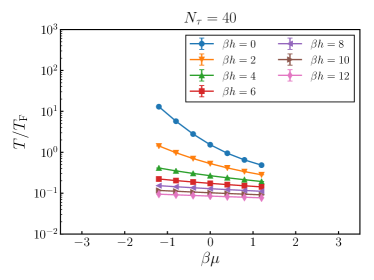
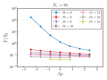
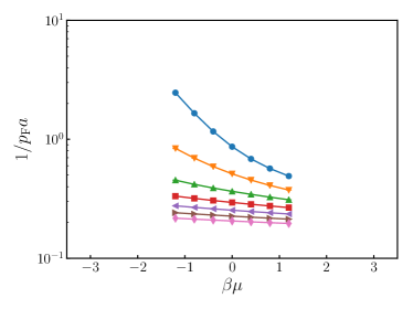
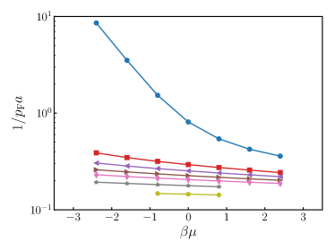
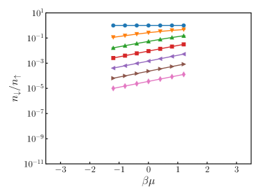
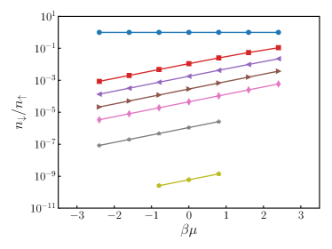
Figure 3: Dimensionless physical parameters $T/T_{\text{F}}$, $1/p_{\text{F}}a$ and the ratio $n_{\downarrow}/n_{\uparrow}$ of particle numbers for $N_{\tau}=40$ (left) and $N_{\tau}=80$ (right).

For each parameter, we computed the ratio of Green’s functions $R(0,na_{\tau})$ defined in Eq. (25) at zero momentum. Numerical results on an $N_{\tau}=40$ lattice at $\beta\mu=0$ for a single configuration are shown in Fig. 4. Qualitative behavior of $R(0,na_{\tau})$ at other $N_{\tau}$ and $\beta\mu$ are same as these results. In the parameter region we swept, $R(0,na_{\tau})$ has a plateau at intermediate imaginary time, which suggests that the energy spectrum is gapped from any possible excited states. In our analysis, we extract the single-particle ground-state energy $E_{0}(0)$ by

$$E_{0}(0)\simeq\frac{1}{a_{\tau}}R(p,\tau=(N_{\tau}-2)a_{\tau})$$ (33)

because the long-time limit as Eq. (25) cannot be taken on a lattice.

After calculating the single-particle energy (33), the polaron energy $U$ is obtained by Eq. (26). In Fig. 5, we show the polaron energy on $N_{\tau}=40$ and $80$ lattices. As the temporal lattice size $N_{\tau}$ becomes large, the system is close to the continuum limit. The color of each point represents the statistical average of $T/T_{\text{F}}$. The lowest temperature is $T/T_{\text{F}}\simeq 0.08$ for $N_{\tau}=40$ and $T/T_{\text{F}}\simeq 0.07$ for $N_{\tau}=80$, respectively. The ratio of particle numbers $n_{\downarrow}/n_{\uparrow}$ varies from $1.0\times 10^{-5}$ to $1.5\times 10^{-1}$ for $N_{\tau}=40$ and $8.4\times 10^{-8}$ to $1.0\times 10^{-1}$ for $N_{\tau}=80$, respectively. The solid line indicates the exact result at zero temperature shown in Eq. (27). For a fixed $N_{\tau}$, the numerical results show similar behavior to Eq. (27) as a function of $1/p_{\text{F}}a$ despite they also depend on $T/T_{\text{F}}$ and $n_{\downarrow}/n_{\uparrow}$. Moreover, the numerical results tend to be close to the exact result at zero temperature when we take the continuum limit. Our result suggests that the polaron energy is insensitive to the temperature and the impurity concentration.

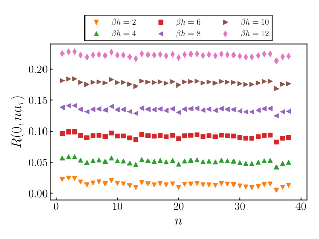
Figure 4: The $\tau$-dependence of the ratio of Green’s functions $R(0,\tau)$ on an $N_{\tau}=40$ lattice at $\beta\mu=0$. $n$ denotes the number for the discretized imaginary time $\tau=na_{\tau}$. Each point in this plot is obtained for a single configuration.

Figure 5: The polaron energy computed by the CLM. The solid line is the exact result at $T=0$ shown in Eq. (27).

VI Summary

We have studied excitation properties of Fermi polarons at finite temperature for the attractive Gaudin-Yang model with large population imbalances using the complex Langevin method, a non-perturbative approach free from the sign problem. We have performed numerical simulations for several chemical potential $\beta\mu$ and Zeeman field $\beta h$, the dimensionless control parameters of the model, and found that our simulation covers wide range of temperature $T/T_{\text{F}}$, strength of the coupling $1/p_{\text{F}}a$ and population imbalance $n_{\downarrow}/n_{\uparrow}$. We have computed the polaron energy as a function of $1/p_{\text{F}}a$. While our result is still away from the zero temperature and single-polaron limit, the computed polaron energy shows similar $(1/p_{\text{F}}a)$-dependence to the exact result at those limits.

The complex Langevin method well works in Gaudin-Yang model even in the presence of the population imbalance. Practically, within our setup, the probability distribution of the drift term always show an exponential fall-off, which means that the problem of wrong convergence does not occur. Moreover, the integrand of path integral is always positive within our simulation from the eigenvalue-analysis. However, it is known that the sign problem is severe in the case of higher dimension Goulko and Wingate (2010). Thus the behavior of the probability distribution of the drift term and the eigenvalues in higher dimension will be investigated as future study.

One interesting application of the complex Langevin method is to study the transition from degenerate Fermi-polaron regime to classical Boltzmann-gas regime of a unitary spin-imbalanced Fermi gas which is found to be a sharp transition by a cold-atom experiment using ⁶Li Fermi gases in a three-dimensional box potential Yan et al. (2019). Also, it is interesting to explore an inhomogeneous pairing phase Rammelmüller et al. (2020, 2021) and in-medium bound states Huber et al. (2019), which cannot be addressed by quantum Monte Carlo simulation due to the sign problem in the mass- and population-imbalanced systems. In order to discuss such phenomena, we need more elaborate estimation of systematic errors. The work in this direction will be presented elsewhere.

References

- von der Linden (1992) W. von der Linden, Physics Reports 220, 53 (1992).
- Pollet (2012) L. Pollet, Reports on Progress in Physics 75, 094501 (2012), arXiv:1206.0781 [cond-mat.quant-gas] .
- Loh et al. (1990) E. Y. Loh, J. E. Gubernatis, R. T. Scalettar, S. R. White, D. J. Scalapino, and R. L. Sugar, Phys. Rev. B 41, 9301 (1990).
- Troyer and Wiese (2005) M. Troyer and U.-J. Wiese, Phys. Rev. Lett. 94, 170201 (2005).
- Muroya et al. (2003) S. Muroya, A. Nakamura, C. Nonaka, and T. Takaishi, Prog. Theor. Phys. 110, 615 (2003), arXiv:hep-lat/0306031 .
- de Forcrand (2009) P. de Forcrand, PoS LAT2009, 010 (2009), arXiv:1005.0539 [hep-lat] .
- Vicari and Panagopoulos (2009) E. Vicari and H. Panagopoulos, Phys. Rept. 470, 93 (2009), arXiv:0803.1593 [hep-th] .
- Krauth et al. (1998) W. Krauth, H. Nicolai, and M. Staudacher, Phys. Lett. B 431, 31 (1998), arXiv:hep-th/9803117 .
- Berges et al. (2007) J. Berges, S. Borsányi, D. Sexty, and I.-O. Stamatescu, Phys. Rev. D 75, 045007 (2007).
- Alexandru et al. (2016) A. Alexandru, G. m. c. Başar, P. F. Bedaque, S. Vartak, and N. C. Warrington, Phys. Rev. Lett. 117, 081602 (2016).
- Blankenbecler et al. (1981) R. Blankenbecler, D. Scalapino, and R. Sugar, Phys. Rev. D 24, 2278 (1981).
- Scalapino and Sugar (1981) D. J. Scalapino and R. L. Sugar, Phys. Rev. B 24, 4295 (1981).
- Sugiyama and Koonin (1986) G. Sugiyama and S. Koonin, Annals of Physics 168, 1 (1986).
- Hirsch (1985) J. E. Hirsch, Phys. Rev. B 31, 4403 (1985).
- Wu and Zhang (2005) C. Wu and S.-C. Zhang, Phys. Rev. B 71, 155115 (2005).
- Li et al. (2015) Z.-X. Li, Y.-F. Jiang, and H. Yao, Phys. Rev. B 91, 241117 (2015), arXiv:1408.2269 [cond-mat.str-el] .
- Li et al. (2016) Z.-X. Li, Y.-F. Jiang, and H. Yao, Phys. Rev. Lett. 117, 267002 (2016), arXiv:1601.05780 [cond-mat.str-el] .
- Wei et al. (2016) Z. C. Wei, C. Wu, Y. Li, S. Zhang, and T. Xiang, Phys. Rev. Lett. 116, 250601 (2016).
- Klauder (1984) J. R. Klauder, Phys. Rev. A29, 2036 (1984).
- Parisi (1983) G. Parisi, Phys. Lett. 131B, 393 (1983).
- Aarts et al. (2010) G. Aarts, E. Seiler, and I.-O. Stamatescu, Phys. Rev. D81, 054508 (2010), arXiv:0912.3360 [hep-lat] .
- Aarts et al. (2011) G. Aarts, F. A. James, E. Seiler, and I.-O. Stamatescu, Eur. Phys. J. C71, 1756 (2011), arXiv:1101.3270 [hep-lat] .
- Nishimura and Shimasaki (2015) J. Nishimura and S. Shimasaki, Phys. Rev. D92, 011501 (2015), arXiv:1504.08359 [hep-lat] .
- Nagata et al. (2016a) K. Nagata, J. Nishimura, and S. Shimasaki, PTEP 2016, 013B01 (2016a), arXiv:1508.02377 [hep-lat] .
- Nagata et al. (2016b) K. Nagata, J. Nishimura, and S. Shimasaki, Phys. Rev. D94, 114515 (2016b), arXiv:1606.07627 [hep-lat] .
- Salcedo (2016) L. L. Salcedo, Phys. Rev. D94, 114505 (2016), arXiv:1611.06390 [hep-lat] .
- Aarts et al. (2017) G. Aarts, E. Seiler, D. Sexty, and I.-O. Stamatescu, JHEP 05, 044 (2017), [Erratum: JHEP01,128(2018)], arXiv:1701.02322 [hep-lat] .
- Nagata et al. (2018) K. Nagata, J. Nishimura, and S. Shimasaki, JHEP 05, 004 (2018), arXiv:1802.01876 [hep-lat] .
- Scherzer et al. (2019) M. Scherzer, E. Seiler, D. Sexty, and I.-O. Stamatescu, Phys. Rev. D99, 014512 (2019), arXiv:1808.05187 [hep-lat] .
- Scherzer et al. (2020) M. Scherzer, E. Seiler, D. Sexty, and I. O. Stamatescu, Phys. Rev. D101, 014501 (2020), arXiv:1910.09427 [hep-lat] .
- Cai et al. (2021) Z. Cai, X. Dong, and Y. Kuang, SIAM J. Sci. Comput. 43, A685 (2021), arXiv:2007.10198 [math.NA] .
- Hayata and Yamamoto (2015) T. Hayata and A. Yamamoto, Phys. Rev. A 92, 043628 (2015), arXiv:1411.5195 [cond-mat.quant-gas] .
- Loheac et al. (2018) A. C. Loheac, J. Braun, and J. E. Drut, Phys. Rev. D 98, 054507 (2018).
- Rammelmüller et al. (2018) L. Rammelmüller, A. C. Loheac, J. E. Drut, and J. Braun, Phys. Rev. Lett. 121, 173001 (2018), arXiv:1807.04664 [cond-mat.quant-gas] .
- Rammelmüller et al. (2020) L. Rammelmüller, J. E. Drut, and J. Braun, SciPost Phys. 9, 14 (2020).
- Rammelmüller et al. (2021) L. Rammelmüller, Y. Hou, J. E. Drut, and J. Braun, Phys. Rev. A 103, 043330 (2021).
- Loheac and Drut (2017) A. C. Loheac and J. E. Drut, Phys. Rev. D 95, 094502 (2017).
- Rammelmüller et al. (2017) L. Rammelmüller, W. J. Porter, J. E. Drut, and J. Braun, Phys. Rev. D 96, 094506 (2017).
- Berger et al. (2021) C. E. Berger, L. Rammelmüller, A. C. Loheac, F. Ehmann, J. Braun, and J. E. Drut, Phys. Rept. 892, 1 (2021), arXiv:1907.10183 [cond-mat.quant-gas] .
- Guan et al. (2013) X.-W. Guan, M. T. Batchelor, and C. Lee, Rev. Mod. Phys. 85, 1633 (2013).
- Schirotzek et al. (2009) A. Schirotzek, C.-H. Wu, A. Sommer, and M. W. Zwierlein, Phys. Rev. Lett. 102, 230402 (2009).
- Nascimbène et al. (2009) S. Nascimbène, N. Navon, K. J. Jiang, L. Tarruell, M. Teichmann, J. McKeever, F. Chevy, and C. Salomon, Phys. Rev. Lett. 103, 170402 (2009).
- Koschorreck et al. (2012) M. Koschorreck, D. Pertot, E. Vogt, B. Fröhlich, M. Feld, and M. Köhl, Nature 485, 619 (2012).
- Cetina et al. (2016) M. Cetina, M. Jag, R. S. Lous, I. Fritsche, J. T. M. Walraven, R. Grimm, J. Levinsen, M. M. Parish, R. Schmidt, M. Knap, and E. Demler, Science 354, 96 (2016), https://science.sciencemag.org/content/354/6308/96.full.pdf .
- Scazza et al. (2017) F. Scazza, G. Valtolina, P. Massignan, A. Recati, A. Amico, A. Burchianti, C. Fort, M. Inguscio, M. Zaccanti, and G. Roati, Phys. Rev. Lett. 118, 083602 (2017).
- Adlong et al. (2020) H. S. Adlong, W. E. Liu, F. Scazza, M. Zaccanti, N. D. Oppong, S. Fölling, M. M. Parish, and J. Levinsen, Phys. Rev. Lett. 125, 133401 (2020).
- Ness et al. (2020) G. Ness, C. Shkedrov, Y. Florshaim, O. K. Diessel, J. von Milczewski, R. Schmidt, and Y. Sagi, Phys. Rev. X 10, 041019 (2020).
- Fritsche et al. (2021) I. Fritsche, C. Baroni, E. Dobler, E. Kirilov, B. Huang, R. Grimm, G. M. Bruun, and P. Massignan, Phys. Rev. A 103, 053314 (2021).
- Massignan et al. (2014) P. Massignan, M. Zaccanti, and G. M. Bruun, Reports on Progress in Physics 77, 034401 (2014).
- McGuire (1966) J. B. McGuire, Journal of Mathematical Physics 7, 123 (1966), https://doi.org/10.1063/1.1704798 .
- He et al. (2016) W.-B. He, Y.-Y. Chen, S. Zhang, and X.-W. Guan, Phys. Rev. A 94, 031604 (2016).
- Klawunn and Recati (2011) M. Klawunn and A. Recati, Phys. Rev. A 84, 033607 (2011).
- Doggen and Kinnunen (2013) E. V. H. Doggen and J. J. Kinnunen, Phys. Rev. Lett. 111, 025302 (2013).
- Tajima et al. (2021) H. Tajima, J. Takahashi, S. I. Mistakidis, E. Nakano, and K. Iida, Atoms 9 (2021), 10.3390/atoms9010018.
- S. Yadong and Z. Huawen (2019) S. Yadong and Z. Huawen, Eur. Phys. J. D 73, 106 (2019).
- Mistakidis et al. (2019) S. I. Mistakidis, G. C. Katsimiga, G. M. Koutentakis, and P. Schmelcher, New Journal of Physics 21, 043032 (2019).
- Yang (1967) C. N. Yang, Phys. Rev. Lett. 19, 1312 (1967).
- Gaudin (1967) M. Gaudin, Physics Letters A 24, 55 (1967).
- Alexandru et al. (2018) A. Alexandru, P. F. Bedaque, and N. C. Warrington, Phys. Rev. D 98, 054514 (2018), arXiv:1805.00125 [hep-lat] .
- Goulko and Wingate (2010) O. Goulko and M. Wingate, Phys. Rev. A 82, 053621 (2010).
- Yan et al. (2019) Z. Yan, P. B. Patel, B. Mukherjee, R. J. Fletcher, J. Struck, and M. W. Zwierlein, Phys. Rev. Lett. 122, 093401 (2019).
- Huber et al. (2019) D. Huber, H.-W. Hammer, and A. G. Volosniev, Phys. Rev. Research 1, 033177 (2019).