Fast and Space-Efficient Construction of AVL Grammars from the LZ77 Parsing

Abstract

Grammar compression is, next to Lempel-Ziv (LZ77) and run-length Burrows-Wheeler transform (RLBWT), one of the most flexible approaches to representing and processing highly compressible strings. The main idea is to represent a text as a context-free grammar whose language is precisely the input string. This is called a straight-line grammar (SLG). An AVL grammar, proposed by Rytter [Theor. Comput. Sci., 2003] is a type of SLG that additionally satisfies the AVL-property: the heights of parse-trees for children of every nonterminal differ by at most one. In contrast to other SLG constructions, AVL grammars can be constructed from the LZ77 parsing in compressed time: $\mathcal{O}(z\log n)$ where $z$ is the size of the LZ77 parsing and $n$ is the length of the input text. Despite these advantages, AVL grammars are thought to be too large to be practical.

We present a new technique for rapidly constructing a small AVL grammar from an LZ77 or LZ77-like parse. Our algorithm produces grammars that are always at least five times smaller than those produced by the original algorithm, and never more than double the size of grammars produced by the practical Re-Pair compressor [Larsson and Moffat, Proc. IEEE, 2000]. Our algorithm also achieves low peak RAM usage. By combining this algorithm with recent advances in approximating the LZ77 parsing, we show that our method has the potential to construct a run-length BWT from an LZ77 parse in about one third of the time and peak RAM required by other approaches. Overall, we show that AVL grammars are surprisingly practical, opening the door to much faster construction of key compressed data structures.

1 Introduction

The increase in the amount of highly compressible data that requires efficient processing in the recent years, particularly in the area of computational genomics [3, 4], has caused a spike of interest in dictionary compression. Its main idea is to reduce the size of the representation of data by finding repetitions in the input and encoding them as references to other occurrences. Among the most popular methods are the Lempel-Ziv (LZ77) compression [31], run-length Burrows-Wheeler transform (RLBWT) [5, 15], and grammar compression [6]. Although in theory, LZ77 and RLBWT are separated by at most a factor of $\mathcal{O}(\log^{2}n)$ (where $n$ is the length of the input text) [14, 19], the gap in practice is usually noticeable (as also confirmed by our experiments). RLBWT is the largest of the three representations in practice, but is also the most versatile, supporting powerful suffix array and suffix tree queries [15]. LZ77, on the other hand, is the smallest, but its functionality includes only the easier LCE, random-access, and pattern matching queries [1, 7, 12, 13, 20]. Grammar compression occupies the middle ground between the two, supporting queries similar to LZ77 [25]. Navarro gives a comprehensive overview of these and related representations in [25, 26].

A major practical concern with these representations – RLBWT in particular – is how to construct them efficiently. Past efforts have focused on engineering efficient general algorithms for constructing the BWT and LZ77 [10, 17, 2, 16], but these are not applicable to the terabyte-scale datasets routinely found, e.g., in modern genomics [4]. Specialized algorithms for highly repetitive datasets have only been investigated recently. Boucher et al. [4] proposed a method for the efficient construction of RLBWT using the concept of prefix-free parsing. The same problem was approached by Policriti and Prezza, and Ohno et al. [28, 27], using a different approach based on the dynamic representation of RLBWT. These methods represent the state of the art in the practical construction of RLBWT.

A different approach to the construction of RLBWT was recently proposed in [19]. The idea is to first compute the (exact or approximate) LZ77 parsing for the text, and then convert this representation into an RLBWT. Crucially, the LZ77 $\rightarrow$ RLBWT conversion takes only $\mathcal{O}(z\operatorname{polylog}n)$ time, i.e. it runs not only in the compressed space but also in compressed time.  The computational bottleneck is therefore shifted to the easier problem of computing or approximating the LZ77, which is the only step taking $\Omega(n)$ time. Internally, this new pipeline consists of three steps: text $\rightarrow$ (approximate) LZ77$\rightarrow$ grammar $\rightarrow$ RLBWT, unsurprisingly aligning with the gradual increase in the size and complexity of these representations. Kosolobov et al. [23] recently proposed a fast and space-efficient algorithm to approximate LZ77, called Re-LZ. The second and third steps in the pipeline, from the LZ77 parse to the RLBWT, have not been implemented. The only known algorithm to convert LZ77 into a grammar in compressed time was proposed by Rytter [29], and is based on the special type of grammars called AVL grammars, whose distinguishing feature is that all subtrees in the parse tree satisfy the AVL property: the tree-heights for children of every nonterminal do not differ by more than one. The algorithm is rather complex, and until now has been considered impractical.

Our Contribution.

Our main contribution is a series of practical improvements to the basic variant of Rytter’s algorithm, and a fast and space-efficient implementation of this improved algorithm. Compared to the basic variant, ours produces a grammar that is always five times smaller, and crucially, the same holds for all intermediate grammars computed during the algorithm, yielding very low peak RAM usage. The resulting grammar is also no more than twice of the smallest existing grammar compressors such as Re-Pair [24]. We further demonstrate that combining our new improved algorithm with Re-LZ opens up a new path to the construction of RLBWT. Our preliminary experiments indicate that at least a three-fold speedup and the same level of reduction in the RAM usage is possible.

The key algorithmic idea in our variant is to delay the merging of intermediate AVL grammars as much as possible to avoid creating nonterminals that are then unused in the final grammar. We dub this variant lazy AVL grammars. We additionally incorporate Karp-Rabin fingerprints [18] to re-write parts of the grammar on-the-fly and further reduce the grammar size. We describe two distinct versions of this technique: greedy and optimal, and demonstrate that both lead to reductions in the grammar size. As a side-result of independent interest, we describe a fast and space-efficient data structure for the dynamic predecessor problem, in which the inserted key is always larger than all other elements currently in the set.

2 Preliminaries

Strings.

For any string $S$, we write $S[i\mathinner{.\,.}j]$, where $1\leq i,j\leq|S|$, to denote a substring of $S$. If $i>j$, we assume $S[i\mathinner{.\,.}j]$ to be the empty string $\varepsilon$. By $[i\mathinner{.\,.}j)$ we denote $[i\mathinner{.\,.}j-1]$. Throughout the paper, we consider a string (text) $T[1\mathinner{.\,.}n]$ of $n\geq 1$ symbols from an integer alphabet $\Sigma=[0\mathinner{.\,.}\sigma)$. By $\mathrm{LCE}(i,i^{\prime})$ we denote the length of the longest common prefix of suffixes $T[i\mathinner{.\,.}n]$ and $T[i^{\prime}\mathinner{.\,.}n]$.

Karp-Rabin Fingerprints.

Let $q$ be a prime number and let $r\in[0\mathinner{.\,.}q-1]$ be chosen uniformly at random. The Karp-Rabin fingerprint of a string $S$ is defined as

$$\Phi(S)=\sum_{i=1}^{|S|}S[i]\cdot r^{|S|-i}\bmod q\ .$$

Clearly, if $T[i\mathinner{.\,.}i+\ell)=T[j\mathinner{.\,.}j+\ell)$ then $\Phi(T[i\mathinner{.\,.}i+\ell))=\Phi(T[j\mathinner{.\,.}j+\ell))$. On the other hand, if $T[i\mathinner{.\,.}i+\ell)\neq T[j\mathinner{.\,.}j+\ell)$ then $\Phi(T[i\mathinner{.\,.}i+\ell))\neq\Phi(T[j\mathinner{.\,.}j+\ell))$ with probability at least $1-\ell/q$ [9]. In our algorithm we are comparing only substrings of $T$ of equal length. Thus, the number of different possible substring comparisons is less than $n^{3}$, and hence for any positive constant $c$, we can set $q$ to be a prime larger than $n^{c+4}$ (but still small enough to fit in $\mathcal{O}(1)$ words) to make the fingerprint function perfect with probability at least $1-n^{-c}$.

LZ77 Compression.

We say that a substring $T[i\mathinner{.\,.}i+\ell)$ is a previous factor if it has an earlier occurrence in $T$, i.e., there exists a position $p\in[1\mathinner{.\,.}i)$ such that $\mathrm{LCE}(i,p)\geq\ell$. An LZ77-like factorization of $T$ is a factorization $T=F_{1}\cdots F_{f}$ into non-empty phrases such that every phrase $F_{j}$ with $|F_{j}|>1$ is a previous factor. Every phrase $F_{j}=T[i\mathinner{.\,.}i+\ell)$ is encoded as a pair $(p,\ell)$, where $p\in[1\mathinner{.\,.}i)$ is such that $\mathrm{LCE}(i,p)\geq\ell$. If there are multiple choices for such $p$, we choose one arbitrarily. The occurrence $T[p\mathinner{.\,.}p+\ell)$ is called the source of the phrase $F_{j}$. If $F_{j}=T[i]$ is not a previous factor, it is encoded as a pair $(T[i],0)$.

The LZ77 factorization [31] (or the LZ77 parsing) of a string $T$ is an LZ77-like factorization constructed by greedily parsing $T$ from left to right into longest possible phrases. More precisely, the $j$th phrase $F_{j}$ is the longest previous factor starting at position $i=1+|F_{1}\cdots F_{j-1}|$. If no previous factor starts there, then $F_{j}=T[i]$. We denote the number of phrases in the LZ77 parsing by $z$. For example, the text bbabaababababaababa has LZ77 parsing $\texttt{b}\cdot\texttt{b}\cdot\texttt{a}\cdot\texttt{ba}\cdot\texttt{aba}\cdot\texttt{bababa}\cdot\texttt{ababa}$ with $z=7$ phrases, and is encoded as a sequence $(\texttt{b},0),(1,1),(\texttt{a},0),(2,2),(3,3),(7,6),(10,5).$

Grammar Compression.

A context-free grammar is a tuple $G=(N,\Sigma,R,S)$, where $N$ is a finite set of nonterminals, $\Sigma$ is a finite set of terminals, and $R\subseteq N\times(N\cup\Sigma)^{*}$ is a set of rules. We assume $N\cap\Sigma=\emptyset$ and $S\in N$. The nonterminal $S$ is called the starting symbol. If $(A,\gamma)\in R$ then we write $A\rightarrow\gamma$. The language of $G$ is set $L(G)\subseteq\Sigma^{*}$ obtained by starting with $S$ and repeatedly replacing nonterminals with their expansions, according to $R$.

A grammar $G=(N,\Sigma,R,S)$ is called a straight-line grammar (SLG) if for any $A\in N$ there is exactly one production with $A$ of the left side, and all nonterminals can be ordered $A_{1},\ldots,A_{|N|}$ such that $S=A_{1}$ and if $A_{i}\rightarrow\gamma$ then $\gamma\in(\Sigma\cup\{A_{i+1}\cup\ldots\cup A_{|N|}\})^{*}$, i.e., the graph of grammar rules is acyclic. The unique $\gamma$ such that $A\rightarrow\gamma$ is called the definition of $A$ and is denoted $\mathrm{rhs}(A)$. In any SLG, for any $u\in(N\cup\Sigma)^{*}$ there exists exactly one $w\in\Sigma^{*}$ that can be obtained from $u$. We call such $w$ the expansion of $u$, and denote $\mathrm{exp}(u)$. We define the parse tree of $A\in N\cup\Sigma$ as a rooted ordered tree $\mathcal{T}(A)$, where each node $v$ is associated to a symbol $\mathrm{sym}(v)\in N\cup\Sigma$. The root of $\mathcal{T}(A)$ is a node $v$ such that $\mathrm{sym}(v)=A$. If $A\in\Sigma$ then $v$ has no children. If $A\in N$ and $\mathrm{rhs}(A)=B_{1}\cdots B_{k}$, then $v$ has $k$ children and the subtree rooted at the $i$th child is a copy of $\mathcal{T}(B_{i})$. The parse tree $\mathcal{T}(G)$ is defined as $\mathcal{T}(S)$. The height of any $A\in N$ is defined as the height of $\mathcal{T}(A)$, and denoted $0pt{A}$.

The idea of grammar compression is, given a text $T$, to compute a small SLG $G$ such that $L(G)=T$. The size of the grammar is measured by the total length of all definitions, and denoted $|G|:=\sum_{A\in N}|\mathrm{rhs}(A)|$. Clearly, it is easy to encode any $G$ in $\mathcal{O}(|G|)$ space: pick an ordering of nonterminals and write down the definitions of all variables with nonterminals replaced by their number in the order.

3 AVL Grammars and the Basic Algorithm

An SLG $G=(N,\Sigma,R,S)$ is said to be in Chomsky normal form, if for every $A\in N$, it holds $\mathrm{rhs}(A)\in\Sigma$ or $\mathrm{rhs}(A)=XY$, where $X,Y\in N$. An SLG in Chomsky normal form is called a straight-line program (SLP). Rytter [29] defines an AVL grammar as an SLP $G=(N,\Sigma,R,S)$ that satisfies the following extra condition: for every $A\in N$ such that $\mathrm{rhs}(A)=XY$, it holds $|0pt{X}|-|0pt{Y}|\leq 1$. This condition guarantees that for every $A\in N$ (in particular for $S\in N$), it holds $0pt{A}=\mathcal{O}(\log|\mathrm{exp}(A)|)$ [29, Lemma 1].

The main result presented in [29] is an algorithm that given a non-self-referential version (in which $T[i\mathinner{.\,.}i+\ell)$ is a previous factor only if there exists $p\in[1\mathinner{.\,.}i-\ell]$ such that $\mathrm{LCE}(i,p)\geq\ell$) of some LZ77-like parsing for a text $T$ of length $n$ consisting of $f$ phrases, computes in $\mathcal{O}(f\log n)$ time an AVL grammar $G$ generating $T$ and satisfying $|G|=\mathcal{O}(f\log n)$. Rytter’s construction was extended to allow self-references in [19, Theorem 6.1]. Our implementation of the basic as well as improved Rytter’s algorithm works for the self-referential variant, but for simplicity here we only describe the algorithm for the non-self-referential variant.

The algorithm in [29] works in $f$ steps. It maintains the dynamically changing AVL grammar $G$ such that after the $k$th step is complete, there exists a nonterminal $P_{k}$ in $G$ such that $\mathrm{exp}(P_{k})=F_{1}\cdots F_{k}$, where $T=F_{1}\cdots F_{f}$ is the input LZ77-like factorization of the input. This implies that at end there exist a nonterminal expanding to $T$. The algorithm does not delete any nonterminals between steps. At the end, it may perform an optional pruning of the grammar to remove the nonterminals not present in the parse tree $\mathcal{T}(P_{f})$. This reduces the grammar size but not the peak memory usage of the algorithm.

The algorithm uses the following three procedures, each of which adds a nonterminal $A$ with a desired expansion $\mathrm{exp}(A)$ to the grammar $G$, along with a bounded number of extra nonterminals:

1. $\mathsf{AddSymbol}(c)$: Given $c\in\Sigma$, add a nonterminal $A$ with $\mathrm{rhs}(A)=c$ to the grammar $G$.

2. $\mathsf{AddMerged}(X,Y)$: Given the identifiers of nonterminals $X,Y$ existing in $G$, add a nonterminal $A$ to $G$ that satisfies $\mathrm{exp}(A)=\mathrm{exp}(X)\mathrm{exp}(Y)$. The difficulty of this operation is ensuring that the updated $G$ remains an AVL grammar. Simply setting $\mathrm{rhs}(A)=XY$ would violate the AVL condition in most cases. Instead, the algorithm performs the procedure similar to the concatenation of AVL trees [21, p. 474], taking $\mathcal{O}(1+|0pt{X}-0pt{Y}|)$ time, and introducing $\mathcal{O}(|0pt{X}-0pt{Y}|)$ extra nonterminals.

3. $\mathsf{AddSubstring}(A,i,j)$: Given the identifier of a nonterminal $A$ existing in $G$, and two positions satisfying $1\leq i\leq j\leq|\mathrm{exp}(A)|$, add a nonterminal $B$ to $G$ that satisfies $\mathrm{exp}(B)=\mathrm{exp}(A)[i\mathinner{.\,.}j]$. To explain how this is achieved, we define the auxiliary procedure $\mathsf{Decompose}(A,i,j)$ that given the same parameters as above, returns the sequence $B_{1},\ldots,B_{q}$ of nonterminals satisfying $\mathrm{exp}(A)[i\mathinner{.\,.}j]=\mathrm{exp}(B_{1})\cdots\mathrm{exp}(B_{q})$. The nonterminals $B_{i}$ are found by performing two root-to-leaf traversals in the parse tree $\mathcal{T}(A)$. This takes $\mathcal{O}(1+0pt{A})=\mathcal{O}(1+\log|\mathrm{exp}(A)|)$ time and ensures $q=\mathcal{O}(\log|\mathrm{exp}(A)|)$. It is easy to see that given $B_{1},\ldots,B_{q}$, we can now obtain $B$ in $\mathcal{O}(1+\log^{2}|\mathrm{exp}(A)|)$ time using $\mathsf{AddMerged}$. In [29], it was however shown that if we always choose the shortest nonterminal to merge with its neighbor, the total runtime is $\mathcal{O}(1+\log|\mathrm{exp}(A)|)$ and only $\mathcal{O}(\log|\mathrm{exp}(A)|)$ extra nonterminals are introduced.

Using the above three procedures, the algorithm in [29] works as follows. Suppose we have already processed the leftmost $k-1$ phrases. The step begins by creating a nonterminal $A_{k}$ satisfying $\mathrm{exp}(A_{k})=F_{k}$. If $|F_{k}|=1$, it uses the procedure $\mathsf{AddSymbol}(F_{k})$. Otherwise, $A_{k}$ is obtained as the output of $\mathsf{AddSubstring}(P_{k-1},p,p+\ell-1)$, where $\ell=|F_{k}|$ and $T[p\mathinner{.\,.}p+\ell)$ is the source of phrase $F_{k}$. Finally, $P_{k}$ is obtained as the output of $\mathsf{AddMerged}(P_{k-1},A_{k})$. A single iteration thus takes $\mathcal{O}(1+\log|F_{1}\cdots F_{k-1}|)=\mathcal{O}(\log n)$ time and adds $\mathcal{O}(\log n)$ extra nonterminals, for total of $\mathcal{O}(f\log n)$ nonterminals over all steps.

4 Optimized Algorithm

Lazy Merging.

We start by observing that the main reason responsible for the large final grammar produced by the algorithm in Section 3 is the requirement that at the end of each step $k\in[1\mathinner{.\,.}f]$, there exist a nonterminal $P_{k}$ satisfying $\mathrm{exp}(P_{k})=F_{1}\cdots F_{k}$. We relax this requirement, and instead require only that at the end of step $k$, there exists a sequence of nonterminals $R_{1},\ldots,R_{m}$ such that $\mathrm{exp}(R_{1})\cdots\mathrm{exp}(R_{m})=F_{1}\cdots F_{k}$. The algorithm explicitly maintains these nonterminals as a sequence of pairs $(\ell_{1},R_{1}),\ldots,(\ell_{m},R_{m})$, where $\ell_{j}=\sum_{i=1}^{j}|\mathrm{exp}(R_{i})|$. The modified algorithm uses the following new procedures:

1. $\mathsf{MergeEnclosed}(i,j)$: Given two positions satisfying $1\leq i\leq j\leq|F_{1}\cdots F_{k-1}|$, add to $G$ a nonterminal $R$ satisfying $\mathrm{exp}(R)=\mathrm{exp}(R_{x})\cdots\mathrm{exp}(R_{y})$, where $x=\min\{t\in[1\mathinner{.\,.}m]:\ell_{t-1}\geq i-1\}$ and $y=\max\{t\in[1\mathinner{.\,.}m]:\ell_{t}\leq j\}$. The positions $x$ and $y$ are found using a binary search. The pairs of the sequence $(\ell_{1},R_{1}),\ldots,(\ell_{m},R_{m})$ at positions between $x$ and $y$ are removed and replaced with a pair ($\ell_{y},R)$. In other words, this procedure merges all the nonterminals from the current root sequence whose expansion is entirely inside the given interval $[i\mathinner{.\,.}j]$. Merging of $R_{x},\ldots,R_{y}$ is performed pairwise, using the $\mathsf{AddMerged}$ procedure. Note, however, that there is no dependence between heights of the adjacent nonterminals (in particular, they do not form a bitonic sequence, like in the algorithm in Section 3), and moreover, their number $\widehat{m}:=y-x+1$ is not bounded. To minimize the number of newly introduced nonterminals, we thus employ a greedy heuristic, that always chooses the nonterminal with the smallest height among the remaining elements, and merges it with the shorter neighbor. We use a list to keep the pointers between neighbors and a binary heap to maintain heights. The merging thus runs in $\mathcal{O}(\widehat{m}\log n)$ time.

2. $\mathsf{DecomposeWithRoots}(i,j)$: Given two positions satisfying $1\leq i\leq j\leq|F_{1}\cdots F_{k-1}|$, this procedure returns a sequence of nonterminals $A_{1},\ldots,A_{q}$ satisfying $(F_{1}\cdots F_{k-1})[i\mathinner{.\,.}j]=\mathrm{exp}(A_{1})\cdots\mathrm{exp}(A_{q})$. First, it computes positions $x$ and $y$, as defined in the description of $\mathsf{MergeEnclosed}$ above. It then returns the result of $\mathsf{Decompose}(R_{x-1},i-\ell_{x-2},\ell_{x-1}-\ell_{x-2})$, followed by $R_{x},\ldots,R_{y}$, followed by the result of $\mathsf{Decompose}(R_{y+1},1,j-\ell_{y})$ (appropriately handling the boundary cases, which for clarity we ignore here). In other words, this procedure finds the sequence of nonterminals that uses as many roots from the sequence $R_{1},\ldots,R_{m}$, as possible, and runs the standard $\mathsf{Decompose}$ for the boundary roots. Letting $\widehat{m}=y-x+1$, it runs in $\mathcal{O}(\widehat{m}+\log n)$ time.

Using the above additional procedures, our algorithm works as follows. Suppose that we have already processed the first $k-1$ phrases. The step begins by computing the sequence of nonterminals $A_{1},\ldots,A_{q}$ satisfying $\mathrm{exp}(A_{1})\cdots\mathrm{exp}(A_{q})=F_{k}$. If $|F_{k}|=1$, we proceed as in Section 3. Otherwise, we first call $\mathsf{MergeEnclosed}(p,p+\ell-1)$, where $\ell=|F_{k}|$ and $T[p\mathinner{.\,.}p+\ell)$ is the source of $F_{k}$. The sequence $A_{1},\ldots,A_{q}$ is then obtained as a result of $\mathsf{DecomposeWithRoots}(p,p+\ell-1)$. Finally, $A_{1},\ldots,A_{q}$, is appended to the roots sequence.

The above algorithm runs in $\mathcal{O}(f\log^{2}n)$ time. To see this, note that first calling $\mathsf{MergeEnclosed}$ ensures that the output size of $\mathsf{DecomposeWithRoots}$ is $\mathcal{O}(\log n)$. Thus, each step appends only $\mathcal{O}(\log n)$ nonterminals to the roots sequence. The total time spend in $\mathsf{MergeEnclosed}$ is thus bounded by $\mathcal{O}(f\log^{2}n)$, dominating the time complexity.

Utilizing Karp-Rabin Fingerprints.

Our second technique is designed to detect the situation in which the algorithm adds a nonterminal $A$ to $G$, when there already exists some $B\in N$ such that $\mathrm{exp}(A)=\mathrm{exp}(B)$. For any $u\in(N\cup\Sigma)^{*}$, we define $\Phi(u)=\Phi(\mathrm{exp}(u))$. Let us assume that there are no collisions between fingerprints. Suppose that given a nonterminal $A\in N$, we can quickly compute $\Phi(A)$, and that given some $x\geq 0$, we can check, if there exists $B\in N$ such that $\Phi(B)=x$. There are two places in the above algorithm (using lazy merging) where we utilize this to reduce the number of nonterminals:

1. Whenever during the greedy merge in $\mathsf{MergeEnclosed}$, we are about to call $\mathsf{AddMerged}$ for the pair of adjacent nonterminals $X$ and $Y$, we instead first compute the fingerprint $x=\Phi(XY)$ of their concatenation, and if there already exists $A\in N$ such that $\Phi(A)=x$, we use $A$ instead, avoiding the call to $\mathsf{AddMerged}$ and the creation of extra nonterminals.

2. Before appending the nonterminals $A_{1},\ldots,A_{q}$ to the roots sequence at the end of the step, we check if there exists an equivalent but shorter sequence $B_{1},\ldots,B_{q^{\prime}}$, i.e., such that $\mathrm{exp}(A_{1})\cdots\mathrm{exp}(A_{q})=\mathrm{exp}(B_{1})\cdots\mathrm{exp}(B_{q^{\prime}})$ and $q^{\prime}<q$. We utilize that $q=\mathcal{O}(\log n)$, and run a quadratic algorithm (based on dynamic programming) to find the optimal (shortest) equivalent sequence. We then use that equivalent sequence in place of $A_{1},\ldots,A_{q}$.

Observe that the above techniques cannot be applied during $\mathsf{AddMerged}$, as the equivalent nonterminal could have a notably shorter/taller parse tree, violating the AVL property. Note also that the algorithm remains correct even when checking if there exists $A\in N$ having $\Phi(A)=x$ returns false negatives. Our implementation uses a parameter $p\in[0\mathinner{.\,.}1]$, which is the probability of storing the mapping from $\Phi(A)$ to $A$, when adding the nonterminal $A$. The value of $p$ is one of the main parameters controlling the time-space trade-off of the algorithm, as well as the size of the final grammar. The mapping of fingerprints to nonterminals is implemented as a hash table.

5 Implementation Details

Storing Sequences.

Our implementation stores many sequences, where the insertion only happens at the end (e.g., the sequence of nonterminals, which are never deleted in the algorithm). A standard approach to this is to use a dynamic array, which is a plain array that doubles its capacity, once it gets full. Such implementation achieves an amortized $\mathcal{O}(1)$ insertion time, but suffers from a high peak RAM usage. On all systems we tried, the reallocation call that extends the array is not in-place. Since the peak RAM usage is critical in our implementation, we thus implemented our own dynamic array, that instead of a single allocated block, keeps a larger number of blocks (we use 32). This significantly reduces the peak RAM usage. We found the slowdown in the access-time to be negligible.

Implementation of the Roots Sequence.

The roots sequence $(\ell_{1},R_{1}),\ldots,(\ell_{m},R_{m})$ undergoes predecessor queries, deletions (at arbitrary positions), and insertions (only at the end). Rather than using an off-the-shelf dynamic predecessor data structure (such as balanced BST), we exploit as follows the fact that insertions happen only at the end.

All roots are stored as a static sequence that only undergoes insertions at the end (using the space efficient dynamic array implementation described above). Deleted elements are marked as deleted, but remain physically in the array. The predecessor query is implemented using a binary search, with skipping of the elements marked as deleted. To ensure that the predecessor queries are efficient, we keep a counter of accesses to the deleted elements. Once it reaches the current array size, we run the “garbage collector” that scans the whole array left-to-right, and removes all the elements marked as deleted, eliminating all gaps. This way, the predecessor query is still efficient, except the complexity becomes amortized.

Computing $\Phi(A)$ and $|\mathrm{exp}(A)|$ for $A\in N$.

During the algorithm, we often need to query the value of $\Phi(A)$ for some nonterminal $A\in N$. In our implementation we utilize 64-bit fingerprints, and hence storing the value $\Phi(A)$ for every nonterminal is expensive. We thus only store $\Phi(A)$ for $A\in N$ satisfying $|\mathrm{exp}(A)|\geq 255$. The number of such elements in $N$ is relatively small. To compute $\Phi(A)$ for any other $A\in N$, we first obtain $\mathrm{exp}(A)$, and then compute $\Phi(A)$ from scratch. This operation is one of the most expensive in our algorithm, and hence whenever possible we avoid doing repeated $\Phi$ queries.

As for the values $|\mathrm{exp}(A)|$, we observe that in most cases, it fits in a single byte. Thus, we designate only a single byte, and whenever $|\mathrm{exp}(A)|\geq 255$, we lookup $|\mathrm{exp}(A)|$ in an array ordered by the number of nonterminal, with access implemented using binary search.

6 Experimental Results

Algorithms.

We performed experiments using the following algorithms:

• Basic-AVLG, our implementation of the algorithm to convert an LZ-like parsing to an AVL grammar proposed by Rytter [29], and outlined in Section 3. Self-overlapping phrases are handled as in the full version of [19, Theorem 6.1]. The implementation uses space-efficient dynamic arrays described in Section 5. This implementation is our baseline.

• Lazy-AVLG, our implementation of the improved version of Basic-AVLG, utilizing lazy merging and Karp-Rabin fingerprints, as described in Section 4. This is the main contribution of our paper. In some of the experiments below, we consider the algorithm with the different probability $p$ of sampling the Karp-Rabin hash of a nonterminal, but our default value (as discussed below) is $p=0.125$. Our implementation (including also Basic-AVLG) is available at https://github.com/dominikkempa/lz77-to-slp.

• Big-BWT, a semi-external algorithm constructing the RLBWT from the input text in $\Omega(n)$ time, proposed by Boucher et al. [4]. As shown in [4], if the input text is highly compressible, the working space of Big-BWT is sublinear in the text length. We use the implementation from https://gitlab.com/manzai/Big-BWT.

• Re-LZ, an external-memory algorithm due to Kosolobov et al. [23] that given a text on disk, constructs its LZ-like parsing in $\Omega(n)$ time [23]. The algorithm is faster than the currently best algorithms to compute the LZ77 parsing. In practice, the ratio $f/z$ between the size $f$ of the resulting parsing and the size $z$ of the LZ77 parsing usually does not exceed 1.5. Its working space is fully tunable and can be specified arbitrarily. We use the implementation from https://gitlab.com/dvalenzu/ReLZ.

• Re-Pair, an $\mathcal{O}(n)$-time algorithm to construct an SLG from the text, proposed by Larsson and Moffat [24]. Although no upper-bound is known on its output size, Re-Pair produces grammars that in practice are smaller than any other grammar-compression method [24]. Its main drawback is that most implementations need $\Theta(n)$ space [11], and hence are not applicable on massive datasets. The only implementation using $o(n)$ space is [22], but it is not practical. There is also work on running Re-Pair on the compressed input [30], but since it already requires the text as a grammar, it is not applicable in our case. In our experiments we therefore use Re-Pair only as a baseline for the achievable grammar size. We use our own implementation, verified to produce grammars comparable to other implementations. We note that there exists recent work on optimizing Re-Pair by utilizing maximal repeats [11]. The decrease in the grammar size, however, requires a potentially more expensive encoding that includes the length of the expansion for every nonterminal. For simplicity, we therefore use the basic version of Re-Pair.

Table 1: Statistics of files used in the experiments, with $n$ denoting text length, $\sigma$ denoting alphabet size, $r$ denoting the number of runs in the BWT, and $z$ denoting the number of phrases in the LZ77 parsing. For convenience, we also show the average BWT run length $n/r$ and the average LZ77 phrase length $n/z$. Each of the symbols in the input texts is encoded using a single byte.

File name	$n$	$\sigma$	$r$	$n/r$	$z$	$n/z$
cere	461 286 644	5	11 574 640	39.85	1 700 630	271.24
coreutils	205 281 778	236	4 684 459	43.82	1 446 468	141.91
einstein.en.txt	467 626 544	139	290 238	1611.18	89 467	5 226.80
influenza	154 808 555	15	3 022 821	51.21	769 286	201.23
dna.001.1	104 857 600	5	1 716 807	61.07	308 355	340.05
english.001.2	104 857 600	106	1 449 518	72.33	335 815	312.24
proteins.001.1	104 857 600	21	1 278 200	82.03	355 268	295.15
sources.001.2	104 857 600	98	1 213 427	86.41	294 994	355.45
chr19.1000	59 125 116 167	5	45 927 063	1287.37	7 423 960	7964.09
kernel	137 438 953 472	229	129 506 377	1061.25	30 222 602	4547.55

All implementations are in C++ and are largely sequential, allowing for a constant number of additional threads used for asynchronous I/O.

We also considered Online-RLBWT, an algorithm proposed by Ohno at al. [27], that given a text in a right-to-left streaming fashion, construct its run-length compressed BWT (RLBWT) in $\mathcal{O}(n\log r)$ time and using only $\mathcal{O}(r\log n)$ bits of working space (the implementation is available from: https://github.com/itomomoti/OnlineRlbwt). In the preliminary experiment we determined that while using only about a third of the memory of Big-BWT (on the 16 GiB prefix of the kernel testfile), the algorithm was about 10x slower than Big-BWT.

Experimental Platform and Datasets.

We performed experiments on a machine equipped with two twelve-core 2.2 GHz Intel Xeon E5-2650v4 CPUs with 30 MiB L3 cache and 512 GiB of RAM. The machine used distributed storage achieving an I/O rate >220 MiB/s (read/write).

The OS was Linux (CentOS 7.7, 64bit) running kernel 3.10.0. All programs were compiled using g++ version 4.8.5 with -O3 -DNDEBUG -march=native options. All reported runtimes are wallclock (real) times. The machine had no other significant CPU tasks running. To measure the peak RAM usage of the programs we used the /usr/bin/time -v command.

The statistics of testfiles used in our experiments are shown in Table 1. Shorter version of files used in the scalability experiments are prefixes of full files. We used the files from the Pizza & Chili repetitive corpus available at http://pizzachili.dcc.uchile.cl/repcorpus.html. We chose a sample of 8 real and pseudo-real files. Since all files are relatively small (less than 512 MiB), we additionally include 2 large repetitive files that we assembled ourselves:

• chr19.1000, a concatenation of 1000 versions of Human chromosome 19. The sequences were obtained from the 1000 Genomes Project [8]. One copy consists of $\sim$58$\times 10^{6}$ symbols.

• kernel, a concatenation of $\sim$10.7 million source files from over 300 versions of the Linux kernel (see http://www.kernel.org/).

Karp-Rabin Sampling Rate.

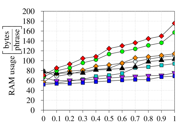
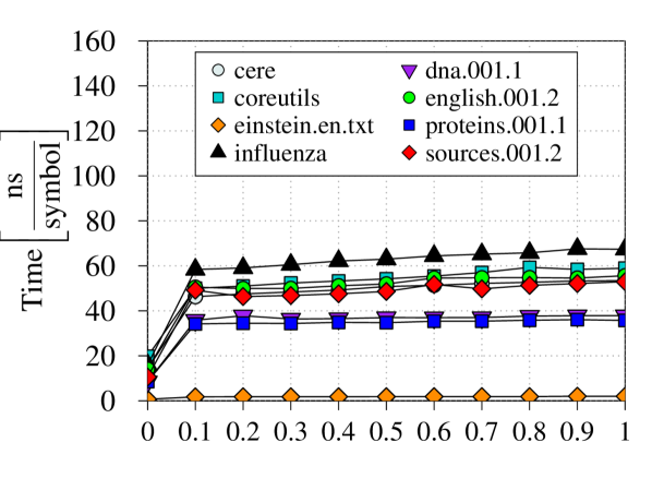
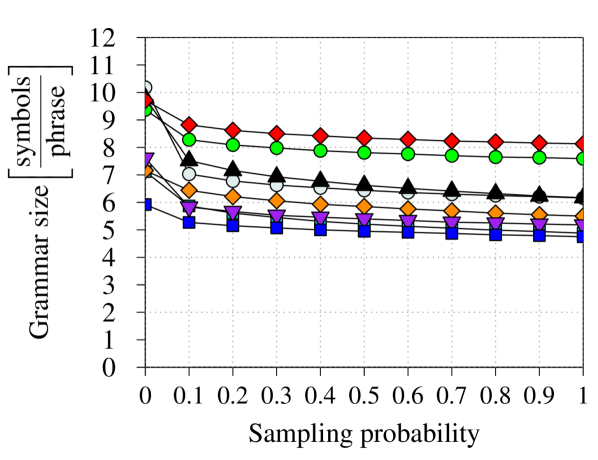
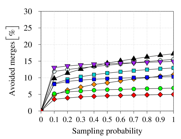
Figure 1: Performance of the Lazy-AVLG algorithm for different values of the parameter $p$ (probability of storing Karp-Rabin fingerprint in the hash table) on the files from Pizza & Chili corpus. The graphs in the top row show the normalized RAM usage (in bytes per phrase of the LZ77 parsing) and the runtime (in ns per symbols of the input text). The bottom row shows the resulting grammar size (the total length of right-hand sides of all productions) divided by $z$, and the percentage of merges avoided during the greedy merge procedure (in %).

The key parameter that controls the runtime, peak RAM usage, and the size of the grammar in our algorithm is the probability $p$ of including the Karp-Rabin fingerprint of a nonterminal in the hash table. In our first experiment, we study the performance of our Lazy-AVLG implementation for different values of the parameter $p$. We tested all values $p\in\{0,0.1,0.2,\ldots,1\}$ and for each we measured the algorithm’s time and memory usage, and the size of the final grammar. The results are given in Figure 1.

While utilizing the Karp-Rabin fingerprints (i.e., setting $p>0$) can notably reduce the final grammar size (up to 40% for the cere file), it is not worth using values $p$ much larger than $0.1$, as it quickly increases the peak RAM usage (e.g., by about 2.3x for the sources.001.2 testfile) and this increase is not repaid significantly in the further grammar reduction. The fourth panel in Figure 1 provides some insight into the reason for this. It shows the percentage of cases, where during the greedy merging of nonterminals enclosed by the source of the phrase, the algorithm is able to avoid merging two nonterminals, and instead use the existing nonterminal. Having some fingerprints in the hash table turns out to be enough to avoid creating between 4-14% of the new nonterminals, but having more does not lead to a significant difference. Since peak RAM usage is the likely limiting factor for this algorithm — a slower algorithm is still usable, but exhaustion of RAM can prevent it running entirely — we chose $p=0.125$ as the default value in our implementation. This is the value used in the next two experiments.

Grammar Size.

In our second experiment, we compare the size of the grammar produced by Lazy-AVLG to Basic-AVLG and Re-Pair. In the comparison we also include the size of the grammar obtained by running Basic-AVLG and removing all nonterminals not reachable from the root. We have run the experiments on 8/10 testfiles, as running Re-Pair on the large files is prohibitively time consuming. The results are given in Figure 2.

Lazy-AVLG produces grammars that are between 1.59x and 2.64x larger than Re-Pair (1.95x on average). The resulting grammar is always at least 5x smaller than produced by Basic-AVLG, and also always smaller than Basic-AVLG (pruned). Importantly, the RAM usage of our conversion is proportional the size of the final grammar, whereas the algorithm to compute the pruned version of Basic-AVLG must first obtain the initial large grammar, increasing peak RAM usage. This is a major practical concern, as described next.

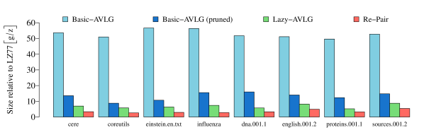
Figure 2: Comparison of the size (measured as the total length of the right hand sides of all nonterminals) of grammars produced by the Basic-AVLG, Lazy-AVLG ($p=0.125$), and Re-Pair algorithms on the files from the Pizza & Chili corpus. Basic-AVLG (pruned) denotes the size of grammar produced by Basic-AVLG with all nonterminals not reachable from the root removed. All sizes are normalized with respect to the size of the LZ77 parsing ($z$).

Application in the Construction of BWT.

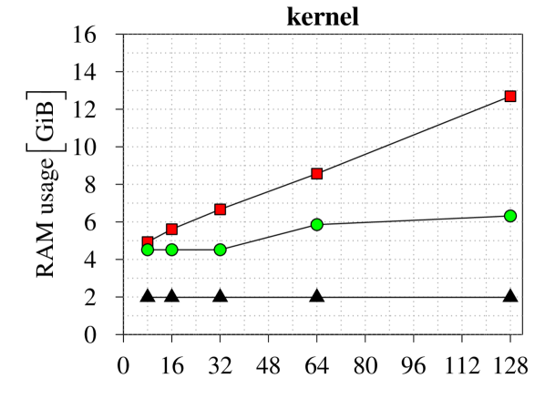
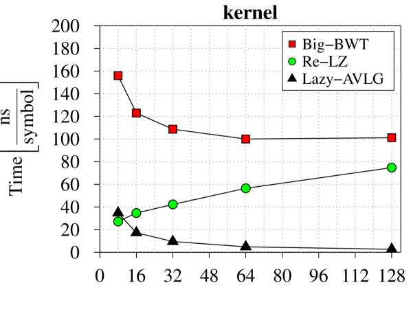
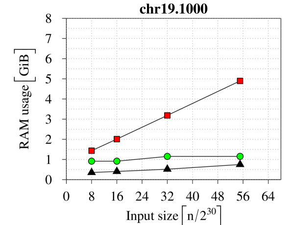
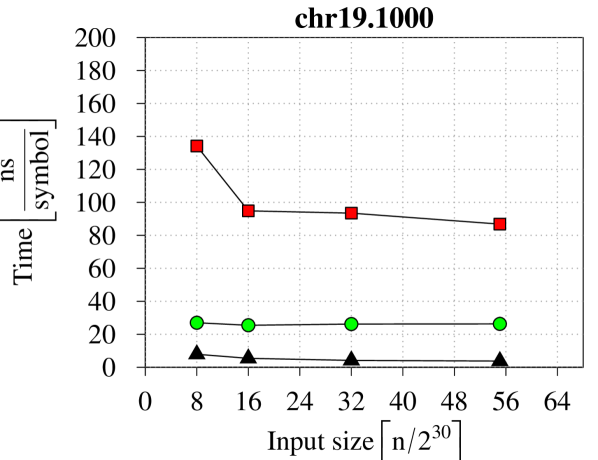
Figure 3: Scalability of Big-BWT compared to Re-LZ and Lazy-AVLG. The graphs on the left show the normalized runtime in ns/char. The graphs on the right show the RAM usage in GiB.

In our third and main experiment, we evaluate the potential of the method to construct RLBWT by first computing/approximating the LZ77-parsing of the text in $\Omega(n)$ time, then converting the resulting compressed representation of $T$ into an RLBWT in $\mathcal{O}(f\operatorname{polylog}n)$ time (where $f$ denotes the number of factors) using the algorithm presented in [19]. The first step of this algorithm is the conversion of the input LZ-compressed text into a straight-line grammar. To our knowledge, the only known approach that achieves runtime within the $\mathcal{O}(f\operatorname{polylog}n)$ time bound is the algorithm of Rytter [29] studied in this paper. Thus, if the approach of [19], has a chance of being practical, the conversion step needs to be efficient. We remark that this step is a necessary but not a sufficient condition, and the remaining components of the algorithm in [19] need to first be engineered before the practicality of this approach is fully determined.

We compared the computational performance of Big-BWT, Re-LZ, and our implementation of Lazy-AVLG with $p=0.125$ (the default value). We have evaluated the runtime and peak RAM usage of these three algorithm on successively longer prefixes of the large testfiles (chr19.1000 and kernel). The RAM use of Re-LZ was set to match RAM use of Big-BWT on the shortest input prefix. To allow a comparison with different methods in the future, we evaluated Lazy-AVLG on the LZ77 parsing rather than on the output of Re-LZ. Thus, to obtain the performance of the pipeline Re-LZ + Lazy-AVLG, one should multiply the runtime and RAM usage of Lazy-AVLG by the approximation ratio $f/z$ of Re-LZ. We have found the value $f/z$ to not exceed $1.05$ on any of the kernel prefixes, and $1.27$ on any of the chr19.1000 prefixes (with the peak reached on the largest prefixes). This puts the RAM use of Lazy-AVLG on the output of Re-LZ still below that of Re-LZ, and its runtime still well below other two programs. The results are given in Figure 3.

At the RAM usage set to stay below that of Big-BWT, the runtime of Re-LZ is always below that of Big-BWT. The reduction is by a factor of at least three for all prefixes of chr19.1000, and by at least 25% for all prefixes of kernel, with the gap decreasing with the prefix length. The runtime of Lazy-AVLG stays significantly below that of both other methods. More importantly, this also holds for Lazy-AVLG’s peak RAM usage. This shows that construction of the RLBWT via LZ-parsing has the potential to be the fastest in practice, especially given that approximation of LZ is the only step requiring $\Omega(n)$ in the pipeline from text to the RLBWT proposed in [19]. We further remark that although the construction of RLBWT has received much attention in recent years, practical approximation of LZ77 is a relatively unexplored topic, potentially offering significant further speedup via new techniques or parallelization. This may be an easier task since, unlike for any BWT construction algorithm, LZ-approximation algorithms need not be exact.

References

- [1] Djamal Belazzougui, Travis Gagie, Paweł Gawrychowski, Juha Kärkkäinen, Alberto Ordóñez Pereira, Simon J. Puglisi, and Yasuo Tabei. Queries on LZ-bounded encodings. In DCC, pages 83–92. IEEE, 2015. doi:10.1109/DCC.2015.69.
- [2] Timo Bingmann, Johannes Fischer, and Vitaly Osipov. Inducing suffix and LCP arrays in external memory. In ALENEX, pages 88–102. SIAM, 2013. doi:10.1137/1.9781611972931.8.
- [3] Christina Boucher, Travis Gagie, Tomohiro I, Dominik Köppl, Ben Langmead, Giovanni Manzini, Gonzalo Navarro, Alejandro Pacheco, and Massimiliano Rossi. PHONI: Streamed matching statistics with multi-genome references. In DCC, pages 193–202. IEEE, 2021. doi:10.1109/DCC50243.2021.00027.
- [4] Christina Boucher, Travis Gagie, Alan Kuhnle, Ben Langmead, Giovanni Manzini, and Taher Mun. Prefix-free parsing for building big BWTs. Algorithms Mol. Biol., 14(1):13:1–13:15, 2019. doi:10.1186/s13015-019-0148-5.
- [5] Michael Burrows and David J. Wheeler. A block-sorting lossless data compression algorithm. Technical Report 124, Digital Equipment Corporation, Palo Alto, California, 1994.
- [6] Moses Charikar, Eric Lehman, Ding Liu, Rina Panigrahy, Manoj Prabhakaran, Amit Sahai, and Abhi Shelat. The smallest grammar problem. Trans. Inf. Theory, 51(7):2554–2576, 2005. doi:10.1109/TIT.2005.850116.
- [7] Francisco Claude and Gonzalo Navarro. Self-indexed grammar-based compression. Fundam. Informaticae, 111(3):313–337, 2011. doi:10.3233/FI-2011-565.
- [8] The 1000 Genomes Project Consortium. A global reference for human genetic variation. Nature, 526:68–74, 2015. doi:10.1038/nature15393.
- [9] Martin Dietzfelbinger, Joseph Gil, Yossi Matias, and Nicholas Pippenger. Polynomial hash functions are reliable. In ICALP, pages 235–246, 1992. doi:10.1007/3-540-55719-9\_77.
- [10] Paolo Ferragina, Travis Gagie, and Giovanni Manzini. Lightweight data indexing and compression in external memory. Algorithmica, 63(3):707–730, 2012.
- [11] Isamu Furuya, Takuya Takagi, Yuto Nakashima, Shunsuke Inenaga, Hideo Bannai, and Takuya Kida. MR-RePair: Grammar compression based on maximal repeats. In DCC, pages 508–517. IEEE, 2019. doi:10.1109/DCC.2019.00059.
- [12] Travis Gagie, Pawel Gawrychowski, Juha Kärkkäinen, Yakov Nekrich, and Simon J. Puglisi. LZ77-based self-indexing with faster pattern matching. In LATIN, pages 731–742. Springer, 2014. doi:10.1007/978-3-642-54423-1\_63.
- [13] Travis Gagie, Paweł Gawrychowski, Juha Kärkkäinen, Yakov Nekrich, and Simon J. Puglisi. A faster grammar-based self-index. In LATA, pages 240–251. Springer, 2012. doi:10.1007/978-3-642-28332-1_21.
- [14] Travis Gagie, Gonzalo Navarro, and Nicola Prezza. On the approximation ratio of Lempel-Ziv parsing. In LATIN, pages 490–503. Springer, 2018. doi:10.1007/978-3-319-77404-6_36.
- [15] Travis Gagie, Gonzalo Navarro, and Nicola Prezza. Fully functional suffix trees and optimal text searching in BWT-runs bounded space. J. ACM, 67(1):1–54, apr 2020. doi:10.1145/3375890.
- [16] Juha Kärkkäinen, Dominik Kempa, and Simon J. Puglisi. Lempel-Ziv parsing in external memory. In DCC, pages 153–162. IEEE, 2014. doi:10.1109/DCC.2014.78.
- [17] Juha Kärkkäinen, Dominik Kempa, and Simon J. Puglisi. Parallel external memory suffix sorting. In CPM, pages 329–342. Springer, 2015. doi:10.1007/978-3-319-19929-0\_28.
- [18] Richard M. Karp and Michael O. Rabin. Efficient randomized pattern-matching algorithms. IBM J. Res. Dev., 31(2):249–260, 1987. doi:10.1147/rd.312.0249.
- [19] Dominik Kempa and Tomasz Kociumaka. Resolution of the Burrows-Wheeler Transform conjecture. In FOCS, pages 1002–1013. IEEE, 2020. Full version: https://arxiv.org/abs/1910.10631. doi:10.1109/FOCS46700.2020.00097.
- [20] Dominik Kempa and Nicola Prezza. At the roots of dictionary compression: String attractors. In STOC, pages 827–840. ACM, 2018. doi:10.1145/3188745.3188814.
- [21] Donald E. Knuth. The Art of Computing, Vol. III, 2nd Ed. Addison-Wesley, 1998.
- [22] Dominik Köppl, Tomohiro I, Isamu Furuya, Yoshimasa Takabatake, Kensuke Sakai, and Keisuke Goto. Re-Pair in small space. Algorithms, 14(1):5, 2021. doi:10.3390/a14010005.
- [23] Dmitry Kosolobov, Daniel Valenzuela, Gonzalo Navarro, and Simon J. Puglisi. Lempel-Ziv-like parsing in small space. Algorithmica, 82(11):3195–3215, 2020. doi:10.1007/s00453-020-00722-6.
- [24] N. Jesper Larsson and Alistair Moffat. Off-line dictionary-based compression. Proceedings of the IEEE, 88(11):1722–1732, 2000.
- [25] Gonzalo Navarro. Indexing highly repetitive string collections, part I: Repetitiveness measures. ACM Comput. Surv., 54(2):29:1–29:31, 2021. doi:10.1145/3434399.
- [26] Gonzalo Navarro. Indexing highly repetitive string collections, part II: Compressed indexes. ACM Comput. Surv., 54(2):26:1–26:32, 2021. doi:10.1145/3432999.
- [27] Tatsuya Ohno, Kensuke Sakai, Yoshimasa Takabatake, Tomohiro I, and Hiroshi Sakamoto. A faster implementation of online RLBWT and its application to LZ77 parsing. J. Discrete Alg., 52-53:18–28, 2018. doi:10.1016/j.jda.2018.11.002.
- [28] Alberto Policriti and Nicola Prezza. LZ77 computation based on the run-length encoded BWT. Algorithmica, 80(7):1986–2011, 2018. doi:10.1007/s00453-017-0327-z.
- [29] Wojciech Rytter. Application of Lempel–Ziv factorization to the approximation of grammar-based compression. Theor. Comput. Sci., 302(1–3):211–222, 2003. doi:10.1016/S0304-3975(02)00777-6.
- [30] Kensuke Sakai, Tatsuya Ohno, Keisuke Goto, Yoshimasa Takabatake, Tomohiro I, and Hiroshi Sakamoto. RePair in compressed space and time. In DCC, pages 518–527. IEEE, 2019. doi:10.1109/DCC.2019.00060.
- [31] Jacob Ziv and Abraham Lempel. A universal algorithm for sequential data compression. Trans. Inf. Theory, 23(3):337–343, 1977. doi:10.1109/TIT.1977.1055714.