Isostables for stochastic oscillators

Abstract

Thomas and Lindner (2014, Phys. Rev. Lett.) defined an asymptotic phase for stochastic oscillators as the angle in the complex plane made by the eigenfunction, having complex eigenvalue with least negative real part, of the backward Kolmogorov (or stochastic Koopman) operator. We complete the phase-amplitude description of noisy oscillators by defining the stochastic isostable coordinate as the eigenfunction with the least negative nontrivial real eigenvalue. Our results suggest a framework for stochastic limit cycle dynamics that encompasses noise-induced oscillations.

Introduction - Nonlinear stochastic oscillations occur throughout natural and engineered systems. Examples include the membrane potential of nerve cells [1, 2], the deflection of sensory organelles [3], the concentration of intracellular calcium [4], the populations of predators and prey [5], chemical reactions [6], climate systems [7] and the intensity of lasers [8]. For a system described by deterministic ordinary differential equations,

$$\frac{d\mathbf{x}}{dt}=\mathbf{f}(\mathbf{x}),\quad\mathbf{x}\in\mathbb{R}^{n}$$ (1)

robust oscillations arise from orbitally stable limit cycle (LC) solutions $\mathbf{x}=\gamma(t)=\gamma(t+T)$ with finite period $T$. The analysis of limit cycle systems through phase-amplitude reduction provides an essentially complete understanding of oscillatory dynamics [9, 10]. By transforming to a phase variable $\theta$, together with $n-1$ amplitude variables $\sigma$ that decay at rates given by the non-trivial Floquet exponents $\lambda_{i}$, ($i=1,\dots,n-1$), the system eq. (1) becomes

$$\dot{\theta}=2\pi/T,\qquad\dot{\sigma}=\Lambda\sigma$$ (2)

with $\Lambda=\text{diag}(\lambda_{1},\dots,\lambda_{n-1})$ [11, 12]. This transformation facilitates the understanding of synchronization, entrainment and control in a broad range of scenarios [13, 14, 15, 16, 17]. Indeed, whereas the level sets of $\theta$ form the well known “isochrons” [18], the LC coincides with the set of points $\{\mathbf{x}\>|\>\sigma(\mathbf{x})=0\}$.

In contrast, in stochastic systems, oscillatory behavior can arise not only from an underlying limit cycle, but in a noise-perturbed spiral–fixed-point system (quasicycle) (see the early example [19]), in systems with an underlying stable heteroclinic orbit driven by random fluctuations [20], or in noisy excitable systems [21]. Incorporating stochastic dynamics fundamentally changes the conceptual foundations underlying the phase-amplitude construction.

Consider the Langevin equation

$$\frac{d\mathbf{X}}{dt}=\mathbf{f}(\mathbf{X})+\mathbf{g}(\mathbf{X})\xi(t)$$ (3)

where $\mathbf{f}$ is an $n$-dimensional vector, $\mathbf{g}$ is an $n\times k$ matrix, $\xi$ is $k$-dimensional white noise with uncorrelated components , $\langle\xi_{i}(t)\xi_{j}(t^{\prime})\rangle=\delta(t-t^{\prime})\delta_{i,j}$, and we interpret the stochastic differential equation in the sense of Itô . For this system, orbits are no longer periodic. The transit times between isochrons or other Poincaré sections are random variables [24, 25]. The classical notion of a “limit cycle”, as a closed, isolated periodic orbit, is no longer well defined, and a shift in perspective is required.

By considering the evolution of ensembles of trajectories, two of us [26] established a generalization of the asymptotic phase to stochastic oscillators, in terms of the slowest decaying complex eigenfunction of the generator $\mathcal{L}^{\dagger}$ of the Markov process eq. (3) . In this Letter we generalize the amplitude coordinate for a planar stochastic oscillator, which we define to be the slowest decaying real eigenfunction of $\mathcal{L}^{\dagger}$. By putting the notion of phase and amplitude on a common basis, we suggest a framework for the study of stochastic oscillatory systems.

Mathematical Preliminaries - As in [26, 28], we describe an ensemble of trajectories through the density

$$\rho(\mathbf{y},t\>|\>\mathbf{x},s)=\frac{1}{|d\mathbf{y}|}\Pr\left\{\mathbf{X}(t)\in[\mathbf{y},\mathbf{y}+d\mathbf{y})\>|\>\mathbf{X}(s)=\mathbf{x}\right\}$$

for $s<t$. The density satisfies Kolmogorov’s equations

$$\frac{\partial}{\partial t}\rho(\mathbf{y},t\>|\>\mathbf{x},s) =\mathcal{L}_{\mathbf{y}}[\rho]=-\nabla_{\mathbf{y}}\cdot\left(\mathbf{f}(\mathbf{y})\rho\right)+\frac{\partial^{2}}{\partial y_{i}y_{j}}\left(D_{ij}(\mathbf{y})\rho\right)$$

$$-\frac{\partial}{\partial s}\rho(\mathbf{y},t\>|\>\mathbf{x},s) =\mathcal{L}^{\dagger}_{\mathbf{x}}[\rho]=\mathbf{f}(\mathbf{x})\cdot\nabla_{\mathbf{x}}\left(\rho\right)+D_{ij}(\mathbf{x})\frac{\partial^{2}}{\partial x_{i}x_{j}}\left(\rho\right)$$

where $D=\frac{1}{2}gg^{\intercal}$. We assume the operators $\mathcal{L}$, $\mathcal{L}^{\dagger}$ admit a complete biorthogonal eigenfunction expansion with respect to the standard inner product $\langle u\>|\>v\rangle=\int_{\mathbb{R}^{n}}u^{*}(\mathbf{x})v(\mathbf{x})\,d\mathbf{x}$

$$\mathcal{L}[P_{\lambda}]=\lambda P_{\lambda},\quad\mathcal{L}^{\dagger}[Q^{*}_{\lambda}]=\lambda Q^{*}_{\lambda},\quad\langle Q_{\lambda}\>|\>P_{\lambda^{\prime}}\rangle=\delta_{\lambda\lambda^{\prime}}.$$ (4)

The eigenmode $P_{0}$ represents the unique stationary probability distribution. The normalization eq. (4) implies $Q_{0}\equiv 1$. The eigenfunction expansion allows us to write the density exactly as

$$\rho(\textbf{y},t|\textbf{x},s)=P_{0}(\textbf{y})+\sum_{\lambda\not=0}e^{\lambda(t-s)}P_{\lambda}(\textbf{y})Q^{*}_{\lambda}(\textbf{x}).$$ (5)

As in [26] we assume that the system is “robustly oscillatory”, meaning (i) the nontrivial eigenvalue with least negative real part $\lambda_{\pm}=\mu\pm i\omega$ is complex (with $\omega>0$), (ii) $|\omega/\mu|\gg 1$, and (iii) for all other eigenvalues $\lambda^{\prime}$, $\Re[\lambda^{\prime}]\leq 2\mu$. These conditions guarantee that we can extract the “stochastic asymptotic phase” $\psi(\mathbf{x})$ from the eigenfunctions $Q^{*}_{\pm}$ corresponding to $\lambda_{\pm}$ by writing $Q^{*}_{\pm}(\mathbf{x})=|Q^{*}_{\pm}|e^{\pm i\psi(\mathbf{x})}$, so $\psi(\mathbf{x})=\pm\arg(Q^{*}_{\pm}(\mathbf{x}))$. Along trajectories, the eigenfunctions $Q^{*}_{\pm}(\mathbf{X}(t))$ evolve in the mean as $\frac{d}{dt}\mathbb{E}[Q_{\pm}^{*}]=\lambda_{\pm}\mathbb{E}[Q_{\pm}^{*}]$, so they behave as a linear focus, oscillating with a period of $2\pi/\omega$ and decaying as $1/|\mu|$ as the density approaches the steady state $P_{0}$.

We now turn to the special case of planar systems . In order to establish the amplitude part of the phase-amplitude reduction, we require the slowest mode describing pure contraction without an associated oscillation. In analogy with [26] we seek the asymptotic amplitude behaviour. Assuming that $\mathcal{L}^{\dagger}$ has a unique, real, least negative eigenvalue, $\lambda_{\text{Floq}}\leq 2\mu<0$, its corresponding eigenfunction, denoted as $\Sigma(\mathbf{x})\equiv Q_{\text{Floq}}(\mathbf{x})$, will decay in the mean as

$$\frac{d}{dt}\mathbb{E}[\Sigma]=\lambda_{\text{Floq}}\mathbb{E}[\Sigma],$$ (6)

cf. eq. (2). We interpret $\Sigma(\mathbf{x})$ as the generalization of the amplitude (or isostable) coordinate for the stochastic system eq. (3). If $\lambda_{2}<\lambda_{\text{Floq}}$ is a more negative real eigenvalue, then the isostable mode dominates the non-oscillatory convergence on time scales $\tau\gtrapprox 1/(\lambda_{\text{Floq}}-\lambda_{2})$.

Moreover, the average of individual trajectories, when transformed to the amplitude variable, shows a purely exponential decay towards the set $\Sigma_{0}\equiv\{\mathbf{x}\>|\>\Sigma(\mathbf{x})=0\}$. Since $\Sigma_{0}$ in the deterministic case corresponds to a LC, it is natural to ask what $\Sigma_{0}$ represents in the stochastic system. To that end, we define a vector field $\mathbf{F}$ via

$$\nabla Q^{*}_{\pm}(\textbf{x})\cdot\mathbf{F}(\textbf{x})=\lambda_{\pm}Q^{*}_{\pm}(\textbf{x}),\enskip\nabla\Sigma(\textbf{x})\cdot\mathbf{F}(\textbf{x})=\lambda_{\text{Floq}}\Sigma(\textbf{x}).$$ (7)

Eq. (7) determines a unique vector field, provided the gradients of $\Sigma(\mathbf{x})$ and $Q^{*}_{\pm}(\mathbf{x})$ are linearly independent at each point $\mathbf{x}$. Although the original deterministic system $\dot{\mathbf{x}}=\mathbf{f}(\mathbf{x})$ may not have oscillatory dynamics, if the full system eq. (3) is robustly oscillatory, the deterministic vector field $\Re[\mathbf{F}]$ will generate a flow with a stable LC, coinciding with $\Sigma_{0}$. Moreover, eq. (7) generates the same amplitude dynamics as $\mathbb{E}[\Sigma]$: pure exponential decay, at rate $\lambda_{\text{Floq}}$, towards $\Sigma_{0}$. In the remainder of the paper (see SI for numerical details) we illustrate the construction of $\Sigma$, $Q^{*}_{\pm}$, $\Re[\mathbf{F}]$ and $\Sigma_{0}$ for a system arising from an underlying LC as well as for noise-induced oscillations and show that it has properties comporting well with physical intuition. Indeed, in the special case of a LC system perturbed by noise, we observe that $\Sigma$ converges to $\sigma$ as $D\to 0$, in each example we have studied.

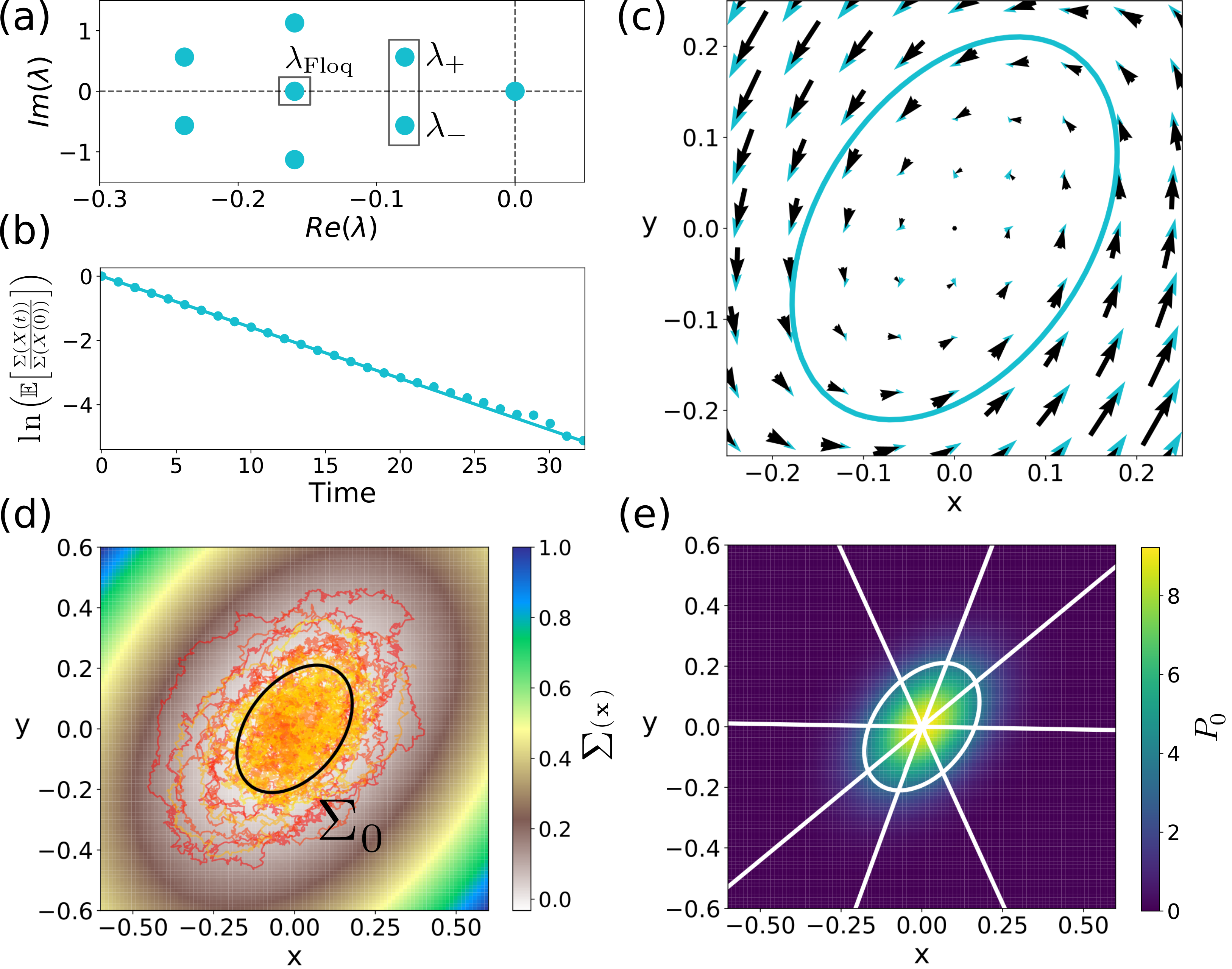
Figure 1: Noisy linear focus eq. (8) with coefficients $A=[0.1598,-0.52;0.7227,-0.319]$ (taken from [30]), and isotropic noise $B=\sqrt{2D}\cdot[1,0;0,1]$. $D=1.25\times 10^{-3}$ for all panels. (a) Eigenvalue spectrum of $\mathcal{L}^{\dagger}$. $\lambda_{\pm}$ and $\lambda_{\text{Floq}}$ are the complex and real eigenvalues having least negative real part. (b) $\ln\left(\mathbb{E}\left[\Sigma(\mathbf{X}(t))/\Sigma(\mathbf{X}(0))\right]\right)$ versus time, showing exponential decay of the mean isostable coordinate. (c) Deterministic vector field (black) and effective vector field $\mathbf{F}(\mathbf{x})$ and its associated effective limit cycle (blue). (d) Isostable function and ten trajectories. Black oval marks the level curve $\Sigma_{0}$. (e) Stationary probability distribution (color coded), eight isochrons (straight lines) and $\Sigma_{0}$ (closed line).

Phase–Amplitude description of a spiral sink - As a first illustration of the isostable construction for a stochastic oscillator we study a two-dimensional Ornstein-Uhlenbeck process with complex eigenvalues at the origin. This system would not oscillate in the absence of noise. Surprisingly, however, phase reduction via the spectral decomposition eq. (4) is well defined [28].

We consider a Langevin equation in the form:

$$\dot{\mathbf{X}}=A\mathbf{X}+B\xi(t)$$ (8)

and assume that the two eigenvalues of $A$ form a complex conjugate pair, $\lambda_{\pm}=\mu\pm i\omega$ (cf. Fig. 1a)

$$A=\begin{pmatrix}\mu&-\omega\\ \omega&\mu\end{pmatrix},\quad B=\begin{pmatrix}B_{11}&B_{12}\\ B_{21}&B_{22}\end{pmatrix}$$ (9)

with $B_{ij}$ arbitrary. The stationary probability density $P_{0}$ of eq. (8) has a planar Gaussian shape (Fig. 1e) [31]. As the spectrum of $\mathcal{L}^{\dagger}$ shows (Fig. 1a) the first complex mode is part of an entire family of harmonics [32]. By using the eigenfunctions $Q^{*}_{\pm}(\textbf{x})=\mathbf{x}_{1}\pm i\mathbf{x}_{2}$ associated to the smallest complex eigenvalue $\lambda_{\pm}=\mu\pm i\omega$, we can define an asymptotic phase function $\psi(\textbf{x})=\arctan(\mathbf{x}_{2}/\mathbf{x}_{1})$ (Fig. 1e) [28]. In addition, we find the eigenfunction $\Sigma(\textbf{x})$ of $\mathcal{L}^{\dagger}$, associated with the least negative nontrivial real eigenvalue $\lambda_{\text{Floq}}$, to be

$$\Sigma(\mathbf{x})=2+\frac{\mu}{\epsilon}(\mathbf{x}^{2}_{1}+\mathbf{x}^{2}_{2}),\qquad\lambda_{\text{Floq}}=2\mu,$$ (10)

depicted in Fig. 1d, with $\epsilon=(B^{2}_{11}+B^{2}_{12}+B^{2}_{21}+B^{2}_{22})/4$. Hence, using $Q_{\pm}^{*}$ and $\Sigma$ we can obtain an analytical expression for the effective vector field $\mathbf{F}(\mathbf{x})$ in eq. (7),

$$\mathbf{F}_{1}(\textbf{x}) =\mu\mathbf{x}_{1}-\omega\mathbf{x}_{2}+2\epsilon\frac{\mathbf{x}_{1}-i\mathbf{x}_{2}}{\mathbf{x}^{2}_{1}+\mathbf{x}^{2}_{2}},$$ (11)

$$\mathbf{F}_{2}(\textbf{x}) =\omega\mathbf{x}_{1}+\mu\mathbf{x}_{2}+2\epsilon\frac{\mathbf{x}_{2}+i\mathbf{x}_{1}}{\mathbf{x}^{2}_{1}+\mathbf{x}^{2}_{2}}.$$

The real part of $\mathbf{F}$, plotted in Fig. 1c, shows how the dissipative effect of the dynamics ($\mu<0$) combines with the expansive effects of the noise ($\epsilon>0$) to give a finite effective radius, (which is evident upon writing eq. (11) in polar coordinates) coinciding with the zero level curve of the isostable function $\Sigma(\mathbf{x})$. That is,

$$\Sigma_{0}(\mathbf{x})=\mathbf{x}^{2}_{1}+\mathbf{x}^{2}_{2}=\frac{2\epsilon}{|\mu|}$$ (12)

with Floquet exponent $\lambda=2\mu=\lambda_{\text{Floq}}$. Hence, averaging an amplitude using $\Sigma(\mathbf{X}(t))$ instead of the original variables $\mathbf{X}(t)$, provides a meaningful asymptotic amplitude $\Sigma_{0}$ (the effective limit cycle) to which trajectories decay exponentially in the mean (see Fig. 1b,d).

Noisy Stuart-Landau (SL) Oscillator - The SL equations capture universal dynamics near a Hopf bifurcation,

$$\dot{\mathbf{X}} =b\mathbf{X}(1-(\mathbf{X}^{2}+\mathbf{Y}^{2}))-\mathbf{Y}(1+ba(\mathbf{X}^{2}+\mathbf{Y}^{2}))+\sqrt{2D_{x}}\xi_{x}(t),$$

$$\dot{\mathbf{Y}} =b\mathbf{Y}(1-(\mathbf{X}^{2}+\mathbf{Y}^{2}))+\mathbf{X}(1+ba(\mathbf{X}^{2}+\mathbf{Y}^{2}))+\sqrt{2D_{y}}\xi_{y}(t)$$

with $a,b=[1,2]\in\mathbb{R}$. In the absence of noise this system has a LC of period $T=2\pi/(1+ba)$ and a Floquet exponent $\lambda=-2b$. To see how isostables capture the effects of noise, in Fig. 2 we study an isotropic ($D_{x,y}=0.1$) and an anisotropic ($D_{x}=0.1$, $D_{y}=2.5\times 10^{-4}$) noise case.

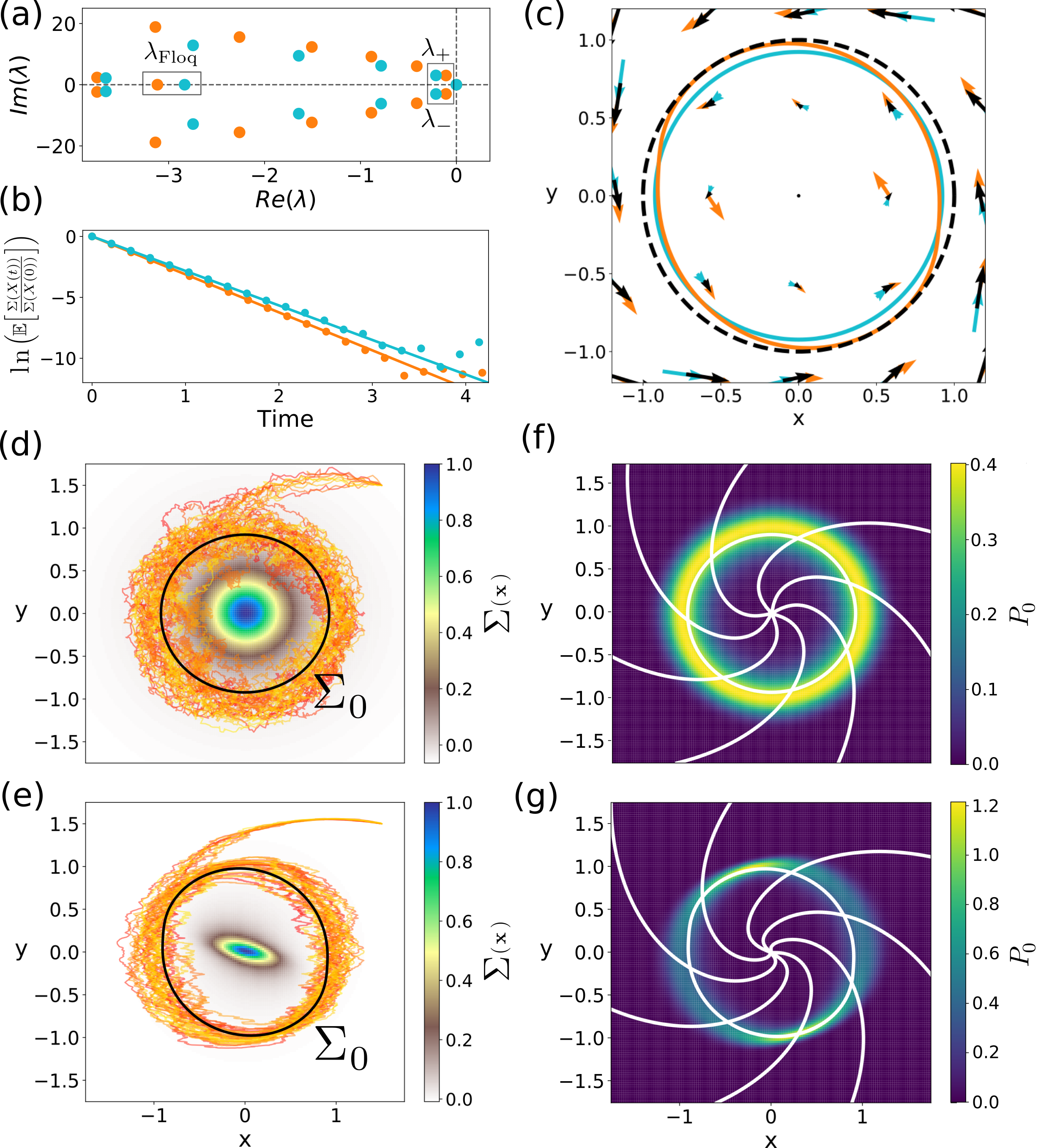
Figure 2: Stuart-Landau oscillator with isotropic noise ($D_{x,y}=0.1$, blue symbols) and anisotropic noise ($D_{x}=0.1$, $D_{y}=2.5\times 10^{-4}$, orange symbols). (a) Eigenvalue spectra of $\mathcal{L}^{\dagger}$ for isotropic and anisotropic noise. (b) $\ln\left(\mathbb{E}\left[\Sigma(\mathbf{X}(t))/\Sigma(\mathbf{X}(0))\right]\right)$ versus time, showing exponential decay of the mean isostable coordinate. (c) Deterministic limit cycle and vector field (black) and effective vector fields $\mathbf{F}$ and their associated effective limit cycles (d-e) Isostable functions and ten trajectories for isotropic (d) and anisotropic (e) noise. (f-g) Stationary probability distribution (color coded), with seven isochrons (straight lines) and $\Sigma_{0}$ (closed line) for isotropic (f) and anisotropic (g) noise.

The isotropic case has larger total noise than the anisotropic case. For this reason, for the anisotropic case, $\Sigma_{0}$ and $\lambda_{\text{Floq}}$ lie nearer their deterministic analogues than for the isotropic case (Fig. 2(a,c)). Under reduced total noise, the real part of the smallest complex eigenvalue pair increases, indicating slower decay of coherent oscillation to the steady-state distribution. We notice the occurrence of a family of eigenvalues $\lambda_{k}\approx\pm i\omega k-\mu k^{2}$ [26, 33]. At the same time, $\lambda_{\text{Floq}}$ becomes more negative, indicating a faster decay of the isostable coordinate (cf. Fig. 2(a,b)). As in the spiral focus system, the slowest decaying real and complex eigenfunctions of the noisy SL system lead to an effective vector field $\mathbf{F}$ that exhibits a stable limit cycle, $\Sigma_{0}$ (panel c). Note the rotational symmetry of $\Sigma_{0}$ in the isotropic case (blue circle in c) versus the lack of symmetry of the anisotropic case (orange ellipse in c); the dashed black curve shows the deterministic SL limit cycle, for comparison. In both cases, the noise reduces the effective radius of the LC. The asymmetry of the anisotropic case appears in all level sets of $\Sigma$, as well as the stationary distribution and isochrons (panel e,g).

Noisy Heteroclinic Oscillator - The underlying vector field of a heteroclinic oscillator creates a closed loop of trajectories connecting a sequence of saddle equilibria [34, 35, 36]. Fig. 3 shows the phase-amplitude analysis of the heteroclinic oscillator system

$$\dot{\mathbf{X}} =\cos(\mathbf{X})\sin(\mathbf{Y})+\alpha\sin(2\mathbf{X})+\sqrt{2D}\xi_{1}(t)$$ (13)

$$\dot{\mathbf{Y}} =-\sin(\mathbf{X})\cos(\mathbf{Y})+\alpha\sin(2\mathbf{Y})+\sqrt{2D}\xi_{2}(t)$$

with $\alpha=0.1$ and reflecting boundary conditions on the domain $-\pi/2\leq\{\mathbf{X},\mathbf{Y}\}\leq\pi/2$. Without noise the system has an attracting heteroclinic cycle. Therefore, it can only sustain robust oscillations in the presence of noise [26]. We study this oscillator for a lower ($D=0.01125$) and for a higher level of noise ($D=0.1$). For the lower level of noise we observe a rightward shift of both the smallest complex eigenvalue, indicating a longer persistence time of the oscillation, and also the smallest real eigenvalue, indicating slower convergence to the stationary state and slower decay of the isostable coordinate towards $\Sigma_{0}$ (cf. 3(a,b)) . At the same time, the mean period increases logarithmically in $D$ (not shown) [20]. The effective vector fields $\mathbf{F}(\mathbf{x})$ differ significantly from the deterministic system $\mathbf{f}(\mathbf{x})$ (panel c), especially near the domain boundaries. Noise causes the effective direction of flow to change, from paralleling the walls, to pointing inwards towards the origin. Consequently, although $\mathbf{f}$ does not support a limit cycle, $\mathbf{F}$ does.

For smaller noise, the stationary distribution (panel f) is pressed tightly against the domain boundaries, and trajectories rarely visit the interior of the domain (panel d). Hence, the zeroth isostable $\Sigma_{0}$ remains close to the domain walls (panel d). For larger noise, the stationary distribution spreads farther from the walls. Due to the reflecting boundaries, trajectories visit all regions of the domain, and $\Sigma_{0}$ contracts partway into the domain interior (panel e). Increasing the noise amplitude reduces significantly the curvature of the isochrons (panel f, g).

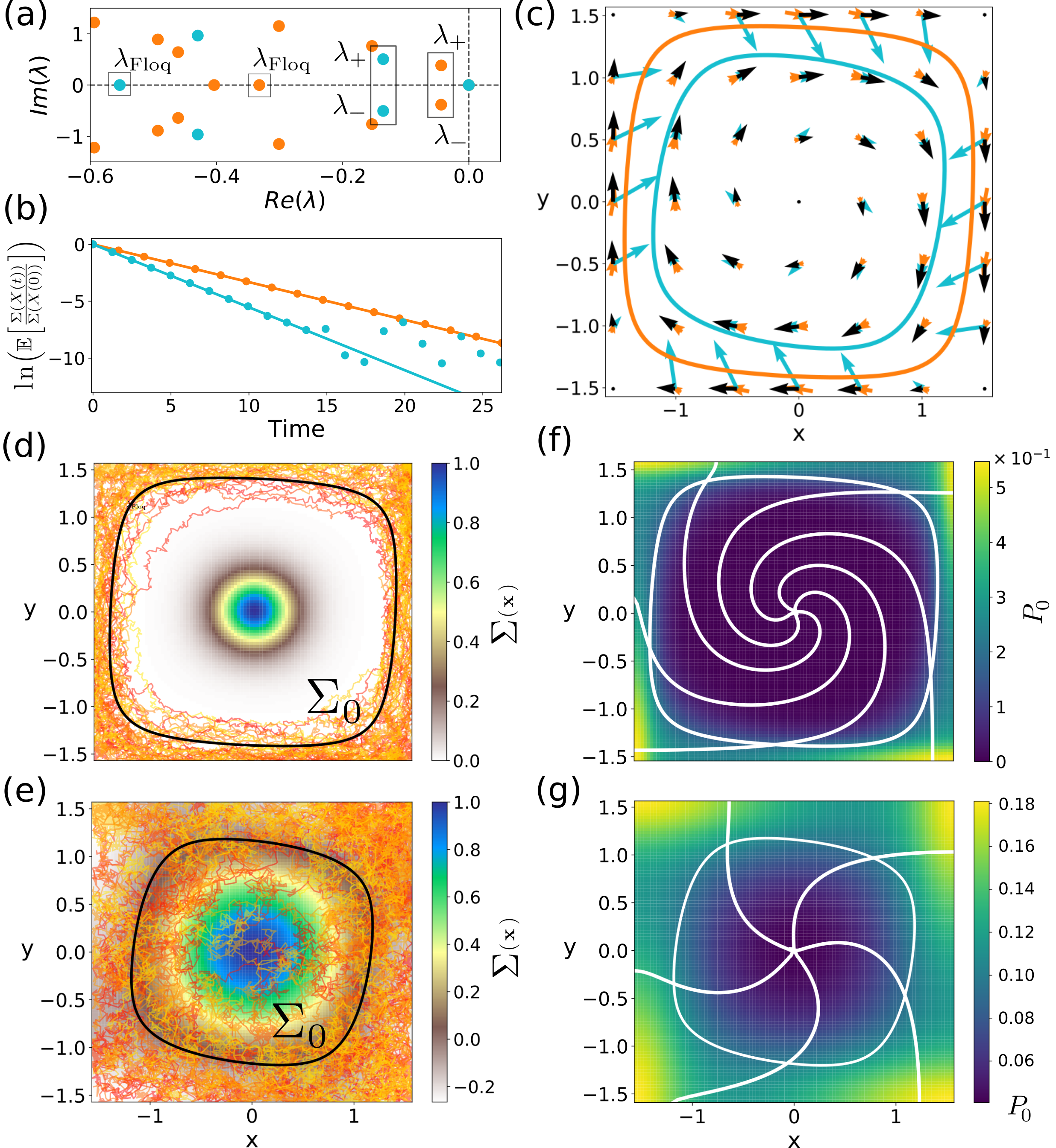
Figure 3: Heteroclinic oscillator with lower ($D=0.01125$, orange symbols) and higher ($D=0.1$, blue symbols) noise. (a) Eigenvalue spectra of $\mathcal{L}^{\dagger}$ for lower and higher noise levels. In this case, reducing $D$ shifts both $\Re[\lambda_{\pm}]$ and $\lambda_{\text{Floq}}$ to the right. (b) $\ln\left(\mathbb{E}\left[\Sigma(\mathbf{X}(t))/\Sigma(\mathbf{X}(0))\right]\right)$ versus time, showing exponential decay of the mean isostable coordinate. (c) Deterministic vector field $\mathbf{f}(\mathbf{x})$ (black) and effective vector fields $\mathbf{F}$ and their associated effective limit cycles. $\mathbf{F}$ and $\mathbf{f}$ differ, especially near the borders. (d-e) Isostable functions and ten trajectories for lower (d) and higher (e) noise. As noise increases, trajectories spread across the phase space, and $\Sigma_{0}$ moves away from the boundaries. (f-g) Stationary probability distribution (color coded), five isochrons (straight lines) and $\Sigma_{0}$ (closed line) for lower (f) and higher (g) noise level.

Discussion - In this Letter we advance the work begun in [26] towards a self-consistent phase-amplitude description of stochastic oscillations. Our methodology applies to stochastic oscillations, even if they are noise induced. By providing an analog of both phase and amplitude, we establish a unified description of deterministic and stochastic oscillations. The zeroth isostable $\Sigma_{0}$ links the deterministic setting, in which the amplitude coordinate obeys $\dot{\sigma}\propto-\sigma$, and the stochastic setting, in which $\dot{\langle\Sigma\rangle}\propto-\langle\Sigma\rangle$. Thus, for an oscillatory stochastic system, trajectories asymptotically approach $\Sigma_{0}$ “in the mean”. In addition to unifying noise-perturbed deterministic LCs and noise-induced oscillations in heteroclinic systems, $\Sigma_{0}$ also captures the mean amplitude dynamics in the case of quasicycles [38, 39, 40, 41]. Together with [26], the framework introduced in this Letter may provide a basis for studying noise-driven oscillations in excitable systems [21], stochastic bifurcations [42], coherence resonance [43, 44], or to construct a physically grounded definition for stochastic limit cycles.

Our results assume a particular structure for the spectrum of $\mathcal{L}^{\dagger}$: the “robustly oscillatory criteria” are met and the initial slowest decaying complex pair entails an entire family of eigenvalues [26]. After this family constituting the phase dynamics, then, the slowest decaying part of the remaining eigenmode decomposition is precisely the least negative real eigenvalue. Moreover, the structure of the spectrum of $\mathcal{L}^{\dagger}$ can also be interpreted in terms of the deterministic phase-amplitude coordinates derived from the eigenfunctions of the Koopman operator [45, 46]. Indeed, the connection between the asymptotic phase for stochastic oscillators introduced in [26] and the Koopman operator has been noted [47, 48, 49]. This connection is not coincidental: the backward Kolmogorov operator at the heart of our analysis, $\mathcal{L}^{\dagger}$, is also the generator of the Markov process, as well as the stochastic Koopman operator [33]. Therefore, beyond its theoretical interest, since our phase-amplitude functions are encoded in the Koopman operator, modern methods for extracting Koopman eigenfunctions from data may lead to practical methods for establishing phase-amplitude coordinates for noisy oscillatory systems in medicine, biology, engineering, economics, control, or other areas [50, 51, 52, 53].

Acknowledgments - Basic Research Program of the National Research University Higher School of Economics and IFISC, UIB-CSIC (APC). NSF grant DMS-2052109, NIH BRAIN Initiative grant R01-NS118606 and the Oberlin College Department of Mathematics (PT).

Supplementary Material
Numerical Results

To obtain the numerical results in the main manuscript, we followed the procedure introduced in [25]. Given a Langevin equation as in eq. (3) in the main manuscript, we first chose a rectangular domain

$$\mathcal{D}=[x^{-},x^{+}]\times[y^{-},y^{+}].$$ (14)

For the spiral sink and the Stuart-Landau oscillator, in which the phase space is unbounded, we use a truncated domain whose size is chosen large enough so that the probability for individual trajectories $\mathbf{X}(t)$ to reach the boundaries is very low. For the special case of the heteroclinic oscillator boundaries are given by the nature of the system.

By discretizing the domain $\mathcal{D}$ in $N$ and $M$ points such that $\Delta x=(x_{+}-x_{-})/N$ and $\Delta y=(y_{+}-y_{-})/M$, we can build $\mathcal{L}^{\dagger}$ (and/or $\mathcal{L}$) by using a standard finite difference scheme. In general we used centered finite differences, that is

$$(\partial_{x}T)_{i,j} =\frac{T_{i+1,j}-T_{i-1,j}}{2\Delta x},$$ (15)

$$(\partial_{xx}T)_{i,j} =\frac{T_{i+1,j}-2T_{i,j}+T_{i-1,j}}{(\Delta x)^{2}}$$ (16)

except at the borders of the domain. For the heteroclinic oscillator, we implemented adjoint reflecting boundary conditions in the borders of the domain. By contrast, for the unbounded systems, since there is no natural border, we just substituted the centered finite difference scheme by a forward (or backward) finite difference scheme. Using adjoint reflecting boundary conditions for these systems yielded numerically very similar results.

After diagonalizing the resulting $(N\cdot M,N\cdot M)$ matrix, we obtain the eigenvalues and the associated eigenfunctions of $\mathcal{L}^{\dagger}$ ($\mathcal{L}$) (for parameter values and resulting eigenvalues see Table 1). We recall that we are not interested in the complete spectrum of $\mathcal{L}^{\dagger}$ ($\mathcal{L}$). For $\mathcal{L}^{\dagger}$ we just consider (and hence present in Figs. 1-3(a)) the part of the spectrum which is relevant for our analysis. That is, we consider the eigenvalue associated with the slowest decaying complex eigenfunction $Q^{*}_{\pm}(\mathbf{x})$ (from which we obtain the asymptotic phase $\psi(\mathbf{x})=\pm\arg(Q^{*}_{\pm}(\mathbf{x})$) and the eigenfunction $\Sigma(\mathbf{x})$ associated with the least negative purely real eigenvalue $\lambda_{\text{Floq}}$. For $\mathcal{L}$ we just consider the eigenmode associated with the eigenvalue $\lambda=0$ which gives the stationary probability distribution $P_{0}$.

	$N$	$M$	$x_{+}$	$x_{-}$	$y_{+}$	$y_{-}$	$\mu$	$\omega$	$\lambda_{\text{Floq}}$
Sp. Sink	151	151	0.6	-0.6	0.6	-0.6	-0.080	0.564	-0.159
SL-iso	151	151	1.75	-1.75	1.75	-1.75	-0.213	3.032	-2.833
SL-ani	151	151	1.75	-1.75	1.75	-1.75	-0.108	3.008	-3.117
Het-low	151	151	$\pi/2$	$-\pi/2$	$\pi/2$	$-\pi/2$	-0.044	0.383	-0.332
Het-high	151	151	$\pi/2$	$-\pi/2$	$\pi/2$	$-\pi/2$	-0.136	0.505	-0.553

Table 1: Numerical values of the parameters and resulting leading eigenvalues for the different stochastic oscillators.

References

- Bryant Jr et al. [1973] H. Bryant Jr, A. R. Marcos, and J. Segundo, J. Neurophysiol 36, 205 (1973).
- Walter et al. [2006] J. T. Walter, K. Alvina, M. D. Womack, C. Chevez, and K. Khodakhah, Nat. Neurosci 9, 389 (2006).
- Martin et al. [2003] P. Martin, D. Bozovic, Y. Choe, and A. J. Hudspeth, J. Neurosci. 23, 4533 (2003).
- Skupin et al. [2008] A. Skupin, H. Kettenmann, U. Winkler, M. Wartenberg, H. Sauer, S. C. Tovey, C. W. Taylor, and M. Falcke, Biophys. J. 94, 2404 (2008).
- McKane and Newman [2005] A. J. McKane and T. J. Newman, Phys. Rev. Lett. 94, 218102 (2005).
- Feistel and Ebeling [1978] R. Feistel and W. Ebeling, Physica A 93, 114 (1978).
- Ganopolski and Rahmstorf [2002] A. Ganopolski and S. Rahmstorf, Phys. Rev. Lett. 88, 038501 (2002).
- McNamara et al. [1988] B. McNamara, K. Wiesenfeld, and R. Roy, Phys. Rev. Lett. 60, 2626 (1988).
- Guillamon and Huguet [2009] A. Guillamon and G. Huguet, SIADS 8, 1005 (2009).
- Wilson and Ermentrout [2019] D. Wilson and B. Ermentrout, Phys. Rev. Lett. 123, 164101 (2019).
- Wilson [2020] D. Wilson, Phys. Rev. E 101 (2020).
- Pérez-Cervera et al. [2020] A. Pérez-Cervera, T. M-Seara, and G. Huguet, Chaos 30, 083117 (2020).
- Pikovsky et al. [2003] A. Pikovsky, J. Kurths, M. Rosenblum, and J. Kurths, Synchronization: a universal concept in nonlinear sciences, 12 (Cambridge university press, 2003).
- Castejón et al. [2013] O. Castejón, A. Guillamon, and G. Huguet, J. Math. Neurosci. 3, 13 (2013).
- Shirasaka et al. [2017] S. Shirasaka, W. Kurebayashi, and H. Nakao, Chaos 27, 023119 (2017).
- Wilson and Ermentrout [2018] D. Wilson and B. Ermentrout, J. Math. Biol. 76, 37 (2018).
- Monga et al. [2019] B. Monga, D. Wilson, T. Matchen, and J. Moehlis, Biol. Cybern. 113, 11 (2019).
- Guckenheimer [1975] J. Guckenheimer, J. Math. Biol. 1, 259 (1975).
- Uhlenbeck and Ornstein [1930] G. E. Uhlenbeck and L. S. Ornstein, Phys. Rev. 36, 823 (1930).
- Giner-Baldó et al. [2017] J. Giner-Baldó, P. J. Thomas, and B. Lindner, J. Stat. Phys. 168, 447 (2017).
- Lindner et al. [2004] B. Lindner, J. Garcıa-Ojalvo, A. Neiman, and L. Schimansky-Geier, Phys. Rep. 392, 321 (2004).
- Note [1] For an example in which , see [54, 55].
- Note [2] We choose the Itô interpretation for its mathematical convenience. For every Stratonovich-interpreted SDE there is an equivalent Itô-interpreted SDE [31]. Thus, choosing between the Itô or the Stratonovich interpretation will not change our framework, which is based on the (uniquely defined) backward Kolmogorov operator.
- Schwabedal and Pikovsky [2013] J. T. Schwabedal and A. Pikovsky, Phys. Rev. Lett. 110, 204102 (2013).
- Cao et al. [2020] A. Cao, B. Lindner, and P. J. Thomas, SIAM J. Appl. Math 80, 422 (2020).